Husimi distribution and phase space analysis of Dicke model quantum phase transition

E. Romera Departamento de Física Atómica, Molecular y Nuclear and Instituto Carlos I de Física Teórica y Computacional, Universidad de Granada, Fuentenueva s/n, 18071 Granada, Spain    R. del Real Departamento de Física Atómica, Molecular y Nuclear, Universidad de Granada, Fuentenueva s/n, 18071 Granada, Spain    M. Calixto Departamento de Matemática Aplicada, Universidad de Granada, Fuentenueva s/n, 18071 Granada, Spain
Abstract

The Husimi distribution is proposed for a phase space analysis of quantum phase transitions in the Dicke model of spin-boson interactions. We show that the inverse participation ratio and Wehrl entropy of the Husimi distribution give sharp signatures of the quantum phase transition. The analysis has been done using two frameworks: a numerical treatment and an analytical variational approximation. Additionally we have proposed a new characterization of the Dicke model quantum phase transition by means of the zeros of the Husimi distribution in the variational approach.

I Introduction

Understanding quantum phase transitions (QPTs) is a relevant fact in quantum many body problems sachdev . QPTs usually occur in a system described by a Hamiltonian of the form H=H0+λH1𝐻subscript𝐻0𝜆subscript𝐻1H=H_{0}+\lambda H_{1}, with H0subscript𝐻0H_{0} exactly solvable, H1subscript𝐻1H_{1} an interaction term and λ𝜆\lambda the corresponding control interaction-strength parameter. The QPT occurs when λ𝜆\lambda reaches some critical value λcsubscript𝜆𝑐\lambda_{c} in which the symmetries (and consequently the properties) of the system change drastically. This is the case of an ensemble of atoms interacting with a single bosonic field mode described by the Dicke Hamiltonian.

Quantum mechanics offers different distributions to characterize phase-space properties Gerry2005 . One is the Wigner function, widely used in quantum optics. Other is the Husimi distribution, which is given by the overlap between a minimal uncertainty (coherent) state and the wavefunction. This distribution is sometimes more convenient because, unlike Wigner distribution, it is non-negative. Husimi distribution has been found useful for a phase-space visualization of a metal-insulator transition aulbach , to analyze quantum chaos in atomic physics monteiro or to analyze models in condensed matter physics weinmann99 . In addition, we would like to point out that the zeros of the Husimi distribution have essential information, in particular, the quantum state can be described by its distribution of zeros Korsch . They are simply the least probable points in phase space and they have been considered as a quantum indicator of classical and quantum chaos 4 ; dando

The Husimi distribution has a great amount of information and it can be useful to consider informational measures as the so-called inverse participation ratio and Wehrl entropy Mintert . Recently, an analysis of QPT in the Dicke model by means of information measures pla11 ; jsm11 ; epl2012 ; physica12 ; renyipra has been done in position and momentum spaces, separately. Here we will do an informational description of the Dicke model QPT in phase space in terms of the inverse participation ration (and higher moments) and the Wehrl entropy of the Husimi distribution and its marginals. Additionally we will investigate the visualization of Dicke model QPT through the zeros of the Husimi distribution.

This article is organized as follows. In Section II we briefly remind the Dicke Hamiltonian, introduce coherent states and the Husimi distribution of the ground state, define moments, Rénnyi-Wehrl entropies and marginals of the Husimi distribution and present numerical results. In Section III we study a variational approximation to the ground state wave function in terms of symmetry-adapted coherent states and analyze the information measures in the thermodynamic limit. Zeros of the Husimi (ansatz) distribution are also computed and graphically represented in order to characterize the QPT.

II Dicke Hamiltonian and Husimi distribution

The single-mode Dicke model is a well studied object in the field of QPTs emaryprl2 ; emarypra ; brandes . In this case the Hamiltonian is given by

H=ω0Jz+ωaa+λ2j(a+a)(J++J),𝐻subscript𝜔0subscript𝐽𝑧𝜔superscript𝑎𝑎𝜆2𝑗superscript𝑎𝑎subscript𝐽subscript𝐽H=\omega_{0}J_{z}+\omega a^{{\dagger}}a+\frac{\lambda}{\sqrt{2j}}(a^{{\dagger}}+a)(J_{+}+J_{-}), (1)

describing an ensemble of N𝑁N two-level atoms with level-splitting ω0subscript𝜔0\omega_{0}, with Jzsubscript𝐽𝑧J_{z}, J±subscript𝐽plus-or-minusJ_{\pm} the angular momentum operators for a pseudospin of length j=N/2𝑗𝑁2j=N/2, and a𝑎a and asuperscript𝑎a^{{\dagger}} are the bosonic operators of the field with frequency ω𝜔\omega. It is well known that there is a QPT at the critical value of the coupling parameter λ=λc=ωω02𝜆subscript𝜆𝑐𝜔subscript𝜔02\lambda=\lambda_{c}=\frac{\sqrt{\omega\omega_{0}}}{2} from the so-called normal phase (λ<λc𝜆subscript𝜆𝑐\lambda<\lambda_{c}) to the superradiant phase (λ>λc𝜆subscript𝜆𝑐\lambda>\lambda_{c}). Let us consider a basis set {|n;j,m|n|j,m}ket𝑛𝑗𝑚tensor-productket𝑛ket𝑗𝑚\left\{|n;j,m\rangle\equiv|n\rangle\otimes|j,m\rangle\right\} of the Hilbert space, with {|n}n=0superscriptsubscriptket𝑛𝑛0\left\{|n\rangle\right\}_{n=0}^{\infty} the number states of the field and {|j,m}m=jjsuperscriptsubscriptket𝑗𝑚𝑚𝑗𝑗\left\{|j,m\rangle\right\}_{m=-j}^{j} the so called Dicke states of the atomic sector. The matrix elements of the Hamiltonian in this basis are:

n;j,m|H|n;j,m=(nω+mω0)δn,nδm,mquantum-operator-productsuperscript𝑛superscript𝑗superscript𝑚𝐻𝑛𝑗𝑚𝑛𝜔𝑚subscript𝜔0subscript𝛿superscript𝑛𝑛subscript𝛿superscript𝑚𝑚\displaystyle\langle n^{\prime};j^{\prime},m^{\prime}|H|n;j,m\rangle=(n\omega+m\omega_{0})\delta_{n^{\prime},n}\delta_{m^{\prime},m}
+λ2j(n+1δn,n+1+nδn,n1)𝜆2𝑗𝑛1subscript𝛿superscript𝑛𝑛1𝑛subscript𝛿superscript𝑛𝑛1\displaystyle+\frac{\lambda}{\sqrt{2j}}(\sqrt{n+1}\delta_{n^{\prime},n+1}+\sqrt{n}\delta_{n^{\prime},n-1})
×(j(j+1)m(m+1)δm,m+1\displaystyle\times(\sqrt{j(j+1)-m(m+1)}\delta_{m^{\prime},m+1}
+j(j+1)m(m1)δm,m1).\displaystyle+\sqrt{j(j+1)-m(m-1)}\delta_{m^{\prime},m-1}). (2)

At this point it is important to note that time evolution preserves the parity eiπ(n+m+j)superscript𝑒𝑖𝜋𝑛𝑚𝑗e^{i\pi(n+m+j)} of a given state |n;j,mket𝑛𝑗𝑚|n;j,m\rangle. That is, the parity operator Π^=eiπ(aa+Jz+j)^Πsuperscript𝑒𝑖𝜋superscript𝑎𝑎subscript𝐽𝑧𝑗\hat{\Pi}=e^{i\pi(a^{\dagger}a+J_{z}+j)} commutes with H𝐻{H} and both operators can then be jointly diagonalized. In particular, the ground state must be even (see later on Eq. (33)).

II.1 Coherent states and Husimi distribution

Let us denote by

|α=e|α|2/2eαa|0=e|α|2/2n=0αnn!|n,|z=(1+|z|2)jezJ+|j,j=(1+|z|2)jm=jj(2jj+m)1/2zj+m|j,m,ket𝛼superscript𝑒superscript𝛼22superscript𝑒𝛼superscript𝑎ket0superscript𝑒superscript𝛼22superscriptsubscript𝑛0superscript𝛼𝑛𝑛ket𝑛ket𝑧superscript1superscript𝑧2𝑗superscript𝑒𝑧subscript𝐽ket𝑗𝑗absentsuperscript1superscript𝑧2𝑗superscriptsubscript𝑚𝑗𝑗superscriptbinomial2𝑗𝑗𝑚12superscript𝑧𝑗𝑚ket𝑗𝑚\begin{array}[]{l}|\alpha\rangle=e^{-|\alpha|^{2}/2}e^{\alpha a^{\dagger}}|0\rangle=e^{-|\alpha|^{2}/2}\sum_{n=0}^{\infty}\frac{\alpha^{n}}{\sqrt{n!}}|n\rangle,\\ |z\rangle=(1+|z|^{2})^{-j}e^{zJ_{+}}|j,-j\rangle=\\ (1+|z|^{2})^{-j}\sum_{m=-j}^{j}\binom{2j}{j+m}^{1/2}z^{j+m}|j,m\rangle,\end{array} (3)

(with α,z𝛼𝑧\alpha,z\in\mathbb{C}) the standard (canonical or Glauber) and spin-j𝑗j Coherent States (CSs) for the photon and the particle sectors, respectively. It is well known (see e.g. Perelomov ) that coherent states form an overcomplete set of the corresponding Hilbert space and fulfill the closure relations or resolutions of the identity:

11\displaystyle 1 =\displaystyle= 1π2|αα|d2α,1𝜋subscriptsuperscript2ket𝛼bra𝛼superscript𝑑2𝛼\displaystyle\frac{1}{\pi}\int_{{\mathbb{R}}^{2}}|\alpha\rangle\langle\alpha|d^{2}\alpha,
11\displaystyle 1 =\displaystyle= 2j+1π2|zz|d2z(1+|z|2)2,2𝑗1𝜋subscriptsuperscript2ket𝑧bra𝑧superscript𝑑2𝑧superscript1superscript𝑧22\displaystyle\frac{2j+1}{\pi}\int_{{\mathbb{R}}^{2}}|z\rangle\langle z|\frac{d^{2}z}{(1+|z|^{2})^{2}}, (4)

with d2w=dRe(w)=dIm(w)superscript𝑑2𝑤𝑑Re𝑤𝑑Im𝑤d^{2}w=d\mathrm{Re}(w)=d\mathrm{Im}(w) the Lebesgue measure on 2superscript2\mathbb{R}^{2} or \mathbb{C}. It is straightforward to see that the probability amplitude of detecting n𝑛n photons and j+m𝑗𝑚j+m excited atoms in |α,z|α|zket𝛼𝑧tensor-productket𝛼ket𝑧|\alpha,z\rangle\equiv|\alpha\rangle\otimes|z\rangle is given by:

φn,m(j)(α,z)=n|αj,m|z=e|α|2/2αnn!(2jj+m)zj+m(1+|z|2)j.superscriptsubscript𝜑𝑛𝑚𝑗𝛼𝑧inner-product𝑛𝛼inner-product𝑗𝑚𝑧superscript𝑒superscript𝛼22superscript𝛼𝑛𝑛binomial2𝑗𝑗𝑚superscript𝑧𝑗𝑚superscript1superscript𝑧2𝑗\varphi_{n,m}^{(j)}(\alpha,z)=\langle n|\alpha\rangle\langle j,m|z\rangle=\frac{e^{-|\alpha|^{2}/2}\alpha^{n}}{\sqrt{n!}}\frac{\sqrt{\binom{2j}{j+m}}z^{j+m}}{(1+|z|^{2})^{j}}. (5)

The ground state vector ψ𝜓\psi will be given as an expansion

|ψ=n=0ncm=jjcnm(j)|n;j,mket𝜓superscriptsubscript𝑛0subscript𝑛𝑐superscriptsubscript𝑚𝑗𝑗superscriptsubscript𝑐𝑛𝑚𝑗ket𝑛𝑗𝑚|\psi\rangle=\sum_{n=0}^{n_{c}}\sum_{m=-j}^{j}c_{nm}^{(j)}|n;j,m\rangle (6)

where the coefficients cnm(j)superscriptsubscript𝑐𝑛𝑚𝑗c_{nm}^{(j)} are calculated by numerical diagonalization of (2) with a given cutoff ncsubscript𝑛𝑐n_{c}. The Husimi distribution of ψ𝜓\psi is then given by

Ψ(α,z)Ψ𝛼𝑧\displaystyle{\Psi}(\alpha,z) =\displaystyle= |α,z|ψ|2superscriptinner-product𝛼𝑧𝜓2\displaystyle|\langle\alpha,z|\psi\rangle|^{2}
=\displaystyle= n,n=0ncm,m=jjcnm(j)c¯nm(j)φn,m(j)(α,z)φn,m(j)(α¯,z¯)superscriptsubscript𝑛superscript𝑛0subscript𝑛𝑐superscriptsubscript𝑚superscript𝑚𝑗𝑗superscriptsubscript𝑐𝑛𝑚𝑗superscriptsubscript¯𝑐superscript𝑛superscript𝑚𝑗superscriptsubscript𝜑𝑛𝑚𝑗𝛼𝑧superscriptsubscript𝜑𝑛𝑚𝑗¯𝛼¯𝑧\displaystyle\sum_{n,n^{\prime}=0}^{n_{c}}\sum_{m,m^{\prime}=-j}^{j}c_{nm}^{(j)}\bar{c}_{n^{\prime}m^{\prime}}^{(j)}\varphi_{n,m}^{(j)}(\alpha,z)\varphi_{n,m}^{(j)}(\bar{\alpha},\bar{z})

and normalized according to:

2j+1π24Ψ(α,z)d2αd2z(1+|z|2)2=1.2𝑗1superscript𝜋2subscriptsuperscript4Ψ𝛼𝑧superscript𝑑2𝛼superscript𝑑2𝑧superscript1superscript𝑧221\frac{2j+1}{\pi^{2}}\int_{\mathbb{R}^{4}}{\Psi}(\alpha,z){d^{2}\alpha}\frac{d^{2}z}{(1+|z|^{2})^{2}}=1. (8)

Before discussing marginals of the Husimi distribution and their properties, let us introduce an important approximation which will simplify things greatly.

II.2 Holstein-Primakoff representation and large pseudospin

We shall make use of the Holstein-Primakoff representation HP of the angular momentum operators J±,Jzsubscript𝐽plus-or-minussubscript𝐽𝑧J_{\pm},J_{z} in terms of the bosonic operators, [b,b]=1𝑏superscript𝑏1[b,b^{\dagger}]=1, given by:

J+=b2jbb,J=2jbbbJz=(bbj).formulae-sequencesubscript𝐽superscript𝑏2𝑗superscript𝑏𝑏subscript𝐽2𝑗superscript𝑏𝑏𝑏subscript𝐽𝑧superscript𝑏𝑏𝑗\begin{array}[]{c}J_{+}=b^{\dagger}\sqrt{2j-b^{\dagger}b},\;\;\;J_{-}=\sqrt{2j-b^{\dagger}b}\;b\\ J_{z}=(b^{\dagger}b-j).\end{array} (9)

For high values of j𝑗j (and fixed bbsuperscript𝑏𝑏b^{\dagger}b), we can approximate J+2jbsimilar-to-or-equalssubscript𝐽2𝑗superscript𝑏J_{+}\simeq\sqrt{2j}\,b^{\dagger} and J2jbsimilar-to-or-equalssubscript𝐽2𝑗𝑏J_{-}\simeq\sqrt{2j}\,b, so that the atomic sector can be practically described by an harmonic oscillator, just like the field sector. Introducing then position and momentum operators for the two bosonic modes as usual:

X=12ω(a+a),PX=iω2(aa),Y=12ω0(b+b),PY=iω02(b+b),𝑋12𝜔superscript𝑎𝑎subscript𝑃𝑋𝑖𝜔2superscript𝑎𝑎𝑌12subscript𝜔0superscript𝑏𝑏subscript𝑃𝑌𝑖subscript𝜔02superscript𝑏𝑏\begin{array}[]{ll}X=\frac{1}{\sqrt{2\omega}}(a^{\dagger}+a),&P_{X}=i\sqrt{\frac{\omega}{2}}(a^{\dagger}-a),\\ Y=\frac{1}{\sqrt{2\omega_{0}}}(b^{\dagger}+b),&P_{Y}=i\sqrt{\frac{\omega_{0}}{2}}(b^{\dagger}+b),\end{array} (10)

the wave function position representation is formally equivalent to that of a set of two coupled harmonic oscillators and can be written as emarypre :

ψ(x,y)=ωω0e12(ωx2+ω0y2)n=0ncm=jjcnm(j)𝜓𝑥𝑦𝜔subscript𝜔0superscript𝑒12𝜔superscript𝑥2subscript𝜔0superscript𝑦2superscriptsubscript𝑛0subscript𝑛𝑐superscriptsubscript𝑚𝑗𝑗superscriptsubscript𝑐𝑛𝑚𝑗\psi(x,y)=\sqrt{\omega\omega_{0}}e^{-\frac{1}{2}(\omega x^{2}+\omega_{0}y^{2})}\sum_{n=0}^{n_{c}}\sum_{m=-j}^{j}c_{nm}^{(j)}
×Hn(ωx)Hj+m(ω0y)2(n+m+j)/2n!(j+m)!absentsubscript𝐻𝑛𝜔𝑥subscript𝐻𝑗𝑚subscript𝜔0𝑦superscript2𝑛𝑚𝑗2𝑛𝑗𝑚\times\frac{H_{n}(\sqrt{\omega}x)H_{j+m}(\sqrt{\omega_{0}}y)}{2^{(n+m+j)/2}\sqrt{n!(j+m)!}} (11)

where we have made use of the definition of

x|ninner-product𝑥𝑛\displaystyle\langle x|n\rangle =\displaystyle= ωe12ωx2Hn(ωx)2nn!π,𝜔superscript𝑒12𝜔superscript𝑥2subscript𝐻𝑛𝜔𝑥superscript2𝑛𝑛𝜋\displaystyle\sqrt{\omega}e^{-\frac{1}{2}\omega x^{2}}\frac{H_{n}(\sqrt{\omega}x)}{\sqrt{2^{n}n!\sqrt{\pi}}}, (12)
y|j,minner-product𝑦𝑗𝑚\displaystyle\langle y|j,m\rangle =\displaystyle= ω0e12ω0y2Hj+m(ω0y)2(j+m)(j+m)!π,subscript𝜔0superscript𝑒12subscript𝜔0superscript𝑦2subscript𝐻𝑗𝑚subscript𝜔0𝑦superscript2𝑗𝑚𝑗𝑚𝜋\displaystyle\sqrt{\omega_{0}}e^{-\frac{1}{2}\omega_{0}y^{2}}\frac{H_{j+m}(\sqrt{\omega_{0}}y)}{\sqrt{2^{(j+m)}(j+m)!\sqrt{\pi}}},

(the Hermite polynomials of degree n𝑛n and j+m𝑗𝑚j+m, respectively) and we have truncated the Hilbert space of the field sector to dimension ncsubscript𝑛𝑐n_{c} looking for the numerical solution and convergence of the eigenproblem Hirchdetallado . This is a very convenient representation that has already been used in Ref. emarypre . Analogously in momentum space:

ψ~(px,py)=1ωω0e12(px2ω+py2ω0)n=0ncm=jj(i)n+m+jcnm(j)~𝜓subscript𝑝𝑥subscript𝑝𝑦1𝜔subscript𝜔0superscript𝑒12superscriptsubscript𝑝𝑥2𝜔superscriptsubscript𝑝𝑦2subscript𝜔0superscriptsubscript𝑛0subscript𝑛𝑐superscriptsubscript𝑚𝑗𝑗superscript𝑖𝑛𝑚𝑗superscriptsubscript𝑐𝑛𝑚𝑗\tilde{\psi}(p_{x},p_{y})=\frac{1}{\sqrt{\omega\omega_{0}}}e^{-\frac{1}{2}(\frac{p_{x}^{2}}{\omega}+\frac{p_{y}^{2}}{\omega_{0}})}\sum_{n=0}^{n_{c}}\sum_{m=-j}^{j}(-i)^{n+m+j}c_{nm}^{(j)}
×Hn(px/ω)Hj+m(py/ω0)2(n+m+j)/2n!(j+m)!.absentsubscript𝐻𝑛subscript𝑝𝑥𝜔subscript𝐻𝑗𝑚subscript𝑝𝑦subscript𝜔0superscript2𝑛𝑚𝑗2𝑛𝑗𝑚\times\frac{H_{n}(p_{x}/\sqrt{\omega})H_{j+m}(p_{y}/\sqrt{\omega_{0}})}{2^{(n+m+j)/2}\sqrt{n!(j+m)!}}. (13)

Moreover, redefining

β2jz,𝛽2𝑗𝑧\beta\equiv\sqrt{2j}\,z, (14)

in (3), it can be seen (see e.g. CScontract1 ; Perelomov ) that spin-j𝑗j coherent states |zket𝑧|z\rangle go over to ordinary coherent states |βe|β|2/2eβb|0ket𝛽superscript𝑒superscript𝛽22superscript𝑒𝛽superscript𝑏ket0|\beta\rangle\equiv e^{-|\beta|^{2}/2}e^{\beta b^{\dagger}}|0\rangle for j1much-greater-than𝑗1j\gg 1 (when identifying |j,j|0ket𝑗𝑗ket0|j,-j\rangle\equiv|0\rangle and |j,m|m+jket𝑗𝑚ket𝑚𝑗|j,m\rangle\equiv|m+j\rangle). Thus, we shall assume the approximation:

|z|β,similar-to-or-equalsket𝑧ket𝛽|z\rangle\simeq|\beta\rangle, (15)

which turns out to be a quite good estimate, even for relatively small values of j𝑗j, for |z|𝑧|z| in a neighborhood of the equilibrium value |ze|<1subscript𝑧𝑒1|z_{e}|<1 in (32). With this approximation, the Husimi distribution (II.1) becomes

Φ(α,β)Φ𝛼𝛽\displaystyle\Phi(\alpha,\beta) =\displaystyle= |α,β|ψ|2superscriptinner-product𝛼𝛽𝜓2\displaystyle|\langle\alpha,\beta|\psi\rangle|^{2}
=\displaystyle= n,n=0ncm,m=jjcnm(j)c¯nm(j)ϕn,m(j)(α,β)ϕn,m(j)(α¯,β¯),superscriptsubscript𝑛superscript𝑛0subscript𝑛𝑐superscriptsubscript𝑚superscript𝑚𝑗𝑗superscriptsubscript𝑐𝑛𝑚𝑗superscriptsubscript¯𝑐superscript𝑛superscript𝑚𝑗superscriptsubscriptitalic-ϕ𝑛𝑚𝑗𝛼𝛽superscriptsubscriptitalic-ϕsuperscript𝑛superscript𝑚𝑗¯𝛼¯𝛽\displaystyle\sum_{n,n^{\prime}=0}^{n_{c}}\sum_{m,m^{\prime}=-j}^{j}c_{nm}^{(j)}\bar{c}_{n^{\prime}m^{\prime}}^{(j)}\phi_{n,m}^{(j)}(\alpha,\beta)\phi_{n^{\prime},m^{\prime}}^{(j)}(\bar{\alpha},\bar{\beta}),

where now

ϕn,m(j)(α,β)=n|αj+m|β=e|α|2/2αnn!e|β|2/2βm+j(m+j)!superscriptsubscriptitalic-ϕ𝑛𝑚𝑗𝛼𝛽inner-product𝑛𝛼inner-product𝑗𝑚𝛽superscript𝑒superscript𝛼22superscript𝛼𝑛𝑛superscript𝑒superscript𝛽22superscript𝛽𝑚𝑗𝑚𝑗\phi_{n,m}^{(j)}(\alpha,\beta)=\langle n|\alpha\rangle\langle j+m|\beta\rangle=\frac{e^{-|\alpha|^{2}/2}\alpha^{n}}{\sqrt{n!}}\frac{e^{-|\beta|^{2}/2}\beta^{m+j}}{\sqrt{(m+j)!}} (17)

with the new normalization

4Φ(α,β)d2αd2βπ2=1.subscriptsuperscript4Φ𝛼𝛽superscript𝑑2𝛼superscript𝑑2𝛽superscript𝜋21\int_{{\mathbb{R}}^{4}}\Phi(\alpha,\beta)\frac{d^{2}\alpha d^{2}\beta}{\pi^{2}}=1. (18)

II.3 Moments, Rényi-Wehrl entropy and marginals of the Husimi distribution

Important quantities to visualize the QPT in the Dicke model across the critical point λcsubscript𝜆𝑐\lambda_{c} will be the ν𝜈\nu-th moments of the Husimi distribution (II.2):

Mj,ν(λ)=4d2αd2βπ2(Φ(α,β))ν.subscript𝑀𝑗𝜈𝜆subscriptsuperscript4superscript𝑑2𝛼superscript𝑑2𝛽superscript𝜋2superscriptΦ𝛼𝛽𝜈M_{j,\nu}(\lambda)=\int_{{\mathbb{R}}^{4}}\frac{d^{2}\alpha d^{2}\beta}{\pi^{2}}(\Phi(\alpha,\beta))^{\nu}. (19)

Note that Mj,1=1subscript𝑀𝑗11M_{j,1}=1 since ΦΦ\Phi is normalized (18). Among all moments we shall single-out the so-called “inverse participation ratio” Pj(λ)=Mj,2(λ)subscript𝑃𝑗𝜆subscript𝑀𝑗2𝜆P_{j}(\lambda)=M_{j,2}(\lambda) which somehow measures the (de-)localization of ΦΦ\Phi across the phase transition. The definition of the moments Mj,νsubscript𝑀𝑗𝜈M_{j,\nu} is not restricted to integer values of ν𝜈\nu. Once Mj,νsubscript𝑀𝑗𝜈M_{j,\nu} are known for all integer ν𝜈\nu, there is a unique analytic extension to complex (and therefore real) ν𝜈\nu, as integers are dense at infinity. The “classical” (versus quantum von Neumann) Rényi-Wehrl entropy is then defined as:

Wj,ν(λ)=11νln(Mj,ν(λ)),subscript𝑊𝑗𝜈𝜆11𝜈subscript𝑀𝑗𝜈𝜆W_{j,\nu}(\lambda)=\frac{1}{1-\nu}\ln(M_{j,\nu}(\lambda)), (20)

which tends to the Wehrl entropy

Wj(λ)=4d2αd2βπ2Φ(α,β)lnΦ(α,β)subscript𝑊𝑗𝜆subscriptsuperscript4superscript𝑑2𝛼superscript𝑑2𝛽superscript𝜋2Φ𝛼𝛽Φ𝛼𝛽W_{j}(\lambda)=-\int_{{\mathbb{R}}^{4}}\frac{d^{2}\alpha d^{2}\beta}{\pi^{2}}\,\,\Phi(\alpha,\beta)\ln\Phi(\alpha,\beta) (21)

when ν1𝜈1\nu\to 1.

In order to differentiate between position and momentum behaviors, we shall study the marginals of the Husimi distribution in each space:

Φ1(α1,β1)subscriptΦ1subscript𝛼1subscript𝛽1\displaystyle\Phi_{1}(\alpha_{1},\beta_{1}) =\displaystyle= 2dα2dβ2πΦ(α1+iα2,β1+iβ2)subscriptsuperscript2𝑑subscript𝛼2𝑑subscript𝛽2𝜋Φsubscript𝛼1𝑖subscript𝛼2subscript𝛽1𝑖subscript𝛽2\displaystyle\int_{{\mathbb{R}}^{2}}\frac{d\alpha_{2}d\beta_{2}}{\pi}\Phi(\alpha_{1}+i\alpha_{2},\beta_{1}+i\beta_{2})
Φ2(α2,β2)subscriptΦ2subscript𝛼2subscript𝛽2\displaystyle\Phi_{2}(\alpha_{2},\beta_{2}) =\displaystyle= 2dα1dβ1πΦ(α1+iα2;β1+iβ2),subscriptsuperscript2𝑑subscript𝛼1𝑑subscript𝛽1𝜋Φsubscript𝛼1𝑖subscript𝛼2subscript𝛽1𝑖subscript𝛽2\displaystyle\int_{{\mathbb{R}}^{2}}\frac{d\alpha_{1}d\beta_{1}}{\pi}\Phi(\alpha_{1}+i\alpha_{2};\beta_{1}+i\beta_{2}), (22)

so that

2dακdβκπΦκ(ακ,βκ)=1,κ=1,2.formulae-sequencesubscriptsuperscript2𝑑subscript𝛼𝜅𝑑subscript𝛽𝜅𝜋subscriptΦ𝜅subscript𝛼𝜅subscript𝛽𝜅1𝜅12\int_{{\mathbb{R}}^{2}}\frac{d\alpha_{\kappa}d\beta_{\kappa}}{\pi}\Phi_{\kappa}(\alpha_{\kappa},\beta_{\kappa})=1,\,\,\kappa=1,2. (23)

We shall also be interested in the moments of marginal distributions

Mj,ν(κ)(λ)=2dακdβκπ(Φκ(ακ,βκ))ν,κ=1,2,formulae-sequencesuperscriptsubscript𝑀𝑗𝜈𝜅𝜆subscriptsuperscript2𝑑subscript𝛼𝜅𝑑subscript𝛽𝜅𝜋superscriptsubscriptΦ𝜅subscript𝛼𝜅subscript𝛽𝜅𝜈𝜅12\displaystyle M_{j,\nu}^{(\kappa)}(\lambda)=\int_{{\mathbb{R}}^{2}}\frac{d\alpha_{\kappa}d\beta_{\kappa}}{\pi}(\Phi_{\kappa}(\alpha_{\kappa},\beta_{\kappa}))^{\nu},\,\kappa=1,2, (24)

specially the marginal inverse participation ratios Pj(κ)(λ)=Mj,2(κ)superscriptsubscript𝑃𝑗𝜅𝜆superscriptsubscript𝑀𝑗2𝜅P_{j}^{(\kappa)}(\lambda)=M_{j,2}^{(\kappa)} and marginal Wehrl entropies

Wj(κ)(λ)=2dακdβκπΦκ(ακ,βκ)lnΦκ(ακ,βκ)superscriptsubscript𝑊𝑗𝜅𝜆subscriptsuperscript2𝑑subscript𝛼𝜅𝑑subscript𝛽𝜅𝜋subscriptΦ𝜅subscript𝛼𝜅subscript𝛽𝜅subscriptΦ𝜅subscript𝛼𝜅subscript𝛽𝜅W_{j}^{(\kappa)}(\lambda)=-\int_{{\mathbb{R}}^{2}}\frac{d\alpha_{\kappa}d\beta_{\kappa}}{\pi}\,\,\Phi_{\kappa}(\alpha_{\kappa},\beta_{\kappa})\ln\Phi_{\kappa}(\alpha_{\kappa},\beta_{\kappa}) (25)

in position (κ=1𝜅1\kappa=1) and momentum (κ=2𝜅2\kappa=2) spaces as a function of the control parameter λ𝜆\lambda. In general, Pj(λ)Pj(1)(λ)Pj(2)(λ)subscript𝑃𝑗𝜆superscriptsubscript𝑃𝑗1𝜆superscriptsubscript𝑃𝑗2𝜆P_{j}(\lambda)\not=P_{j}^{(1)}(\lambda)P_{j}^{(2)}(\lambda) and Wj(λ)Wj(1)(λ)+Wj(2)(λ)subscript𝑊𝑗𝜆superscriptsubscript𝑊𝑗1𝜆superscriptsubscript𝑊𝑗2𝜆W_{j}(\lambda)\not=W_{j}^{(1)}(\lambda)+W_{j}^{(2)}(\lambda), but these quantities are approximately equal for high j𝑗j except in a close neighborhood of λcsubscript𝜆𝑐\lambda_{c} aulbach .

In Appendix A we provide a connection with other phase-space formulas for marginal distributions in position and momentum coordinates (10). This approach has been used in aulbach to visualize the metal-insulator QPT described by the Aubry-André model. We also make use of this representation to make numerical calculations more maneuverable.

II.4 Numerical Results

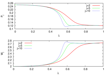
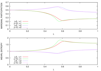
Firstly we have calculated the participation ratio Pj(λ)subscript𝑃𝑗𝜆P_{j}(\lambda) and the Wherl entropy Wj(λ)subscript𝑊𝑗𝜆W_{j}(\lambda) for different values of λ𝜆\lambda. The computed results are given in Fig. 1 where we present Pj(λ)subscript𝑃𝑗𝜆P_{j}(\lambda) and Wj(λ)subscript𝑊𝑗𝜆W_{j}(\lambda) for j=2,5,𝑗25j=2,5, 101010 and for ω=ω0=1𝜔subscript𝜔01\omega=\omega_{0}=1 (for which λc=0.5subscript𝜆𝑐0.5\lambda_{c}=0.5). Notice that the inverse partipation ratio (top pannel) is around 1/4141/4 in the normal phase decreasing around the critical point to reach the value 1/8181/8 in the superradiant phase. We can see that the change in the participation ratio is suddener as j𝑗j increases. The Wherl entropy (botton panel) is approximately 222 in the normal phase and around 2+ln2222+\ln 2 in the superradiant phase changing suddenly (suddener as j𝑗j increases) around the critical point. For completeness we have represented the computed marginal quantities in figure 2.
Refer to caption
Figure 1: Inverse participation ratio Pj(λ)subscript𝑃𝑗𝜆P_{j}(\lambda) and entropy in phase space Wj(λ)subscript𝑊𝑗𝜆W_{j}(\lambda) for j=5𝑗5j=5 and j=10𝑗10j=10 and ω0=ω=1subscript𝜔0𝜔1\omega_{0}=\omega=1 as a function of λ𝜆\lambda
Refer to caption
Figure 2: Inverse participation ratio Pj(i)λ)P_{j}^{(i)}\lambda) and entropy in phase space Wj(i)(λ)superscriptsubscript𝑊𝑗𝑖𝜆W_{j}^{(i)}(\lambda) for j=5𝑗5j=5 and j=10𝑗10j=10, i=1,𝑖1i=1, 222 and ω0=ω=1subscript𝜔0𝜔1\omega_{0}=\omega=1 as a function of λ𝜆\lambda

III Variational aproximation and the thermodynamic limit

Now we present analytical expressions for Husimi’s distribution, its marginals, moments and entropies using trial states expressed in terms of “parity-symmetry-adapted” CSs introduced by Castaños et al. casta1 ; casta2 , which turn out to be an excellent approximation to the exact quantum solution of the ground (+) and first excited (–) states of the Dicke model.

III.1 Symmetry-adapted coherent states and their Husimi distribution

Using the direct product |α,z|α|zket𝛼𝑧tensor-productket𝛼ket𝑧|\alpha,z\rangle\equiv|\alpha\rangle\otimes|z\rangle as a ground-state ansatz, one can easily compute the mean energy

(α,z)=α,z|H|α,z=ω|α|2+jω0|z|21|z|2+1+λ2j(α+α¯)z¯+z|z|2+1,𝛼𝑧quantum-operator-product𝛼𝑧𝐻𝛼𝑧absent𝜔superscript𝛼2𝑗subscript𝜔0superscript𝑧21superscript𝑧21𝜆2𝑗𝛼¯𝛼¯𝑧𝑧superscript𝑧21\begin{array}[]{l}{\cal H}(\alpha,z)=\langle\alpha,z|H|\alpha,z\rangle\\ =\omega|\alpha|^{2}+j\omega_{0}\frac{|z|^{2}-1}{|z|^{2}+1}+{\lambda}{\sqrt{2j}}(\alpha+\bar{\alpha})\frac{\bar{z}+z}{|z|^{2}+1},\\ \end{array} (26)

which defines a four-dimensional “energy surface”. Minimizing with respect to these four coordinates gives the equilibrium points:

αesubscript𝛼𝑒\displaystyle\alpha_{e} =\displaystyle= {0,ifλ<λc2jω0ωλλc1(λλc)4,ifλλccases0if𝜆subscript𝜆𝑐2𝑗subscript𝜔0𝜔𝜆subscript𝜆𝑐1superscript𝜆subscript𝜆𝑐4if𝜆subscript𝜆𝑐\displaystyle\left\{\begin{array}[]{ll}0,&\mathrm{if}\,\lambda<\lambda_{c}\\ -\sqrt{2j}\sqrt{\frac{\omega_{0}}{\omega}}\frac{\lambda}{\lambda_{c}}\sqrt{1-\left(\frac{\lambda}{\lambda_{c}}\right)^{-4}},&\mathrm{if}\,\lambda\geq\lambda_{c}\end{array}\right. (29)
zesubscript𝑧𝑒\displaystyle z_{e} =\displaystyle= {0,ifλ<λcλλc(λλc)1λλc+(λλc)1,ifλλccases0if𝜆subscript𝜆𝑐𝜆subscript𝜆𝑐superscript𝜆subscript𝜆𝑐1𝜆subscript𝜆𝑐superscript𝜆subscript𝜆𝑐1if𝜆subscript𝜆𝑐\displaystyle\left\{\begin{array}[]{ll}0,&\mathrm{if}\,\lambda<\lambda_{c}\\ \sqrt{\frac{\frac{\lambda}{\lambda_{c}}-\left(\frac{\lambda}{\lambda_{c}}\right)^{-1}}{\frac{\lambda}{\lambda_{c}}+\left(\frac{\lambda}{\lambda_{c}}\right)^{-1}}},&\mathrm{if}\,\lambda\geq\lambda_{c}\end{array}\right. (32)

Note that αesubscript𝛼𝑒\alpha_{e} and zesubscript𝑧𝑒z_{e} are real and non-zero above the critical point λcsubscript𝜆𝑐\lambda_{c} (i.e., in the superradiant phase).

Although the direct product |α,zket𝛼𝑧|\alpha,z\rangle gives a good variational approximation to the ground state mean energy in the thermodynamic limit j𝑗j\to\infty, it does not capture the correct behavior for other ground state properties sensitive to the parity symmetry Π^^Π\hat{\Pi} of the Hamiltonian (1) like, for instance, uncertainty and entropy measures. This is why parity-symmetry adapted coherent states are introduced. Indeed, a far better variational description of the ground (resp. first-excited) state is given in terms of the even-(resp. odd)-parity coherent states

|ψ±=|α,z,±=|α|z±|α|z𝒩±(α,z),ketsubscript𝜓plus-or-minusket𝛼𝑧plus-or-minusplus-or-minustensor-productket𝛼ket𝑧tensor-productket𝛼ket𝑧subscript𝒩plus-or-minus𝛼𝑧|\psi_{\pm}\rangle=|\alpha,z,\pm\rangle=\frac{|\alpha\rangle\otimes|z\rangle\pm|-\alpha\rangle\otimes|-z\rangle}{{\mathcal{N}}_{\pm}(\alpha,z)}, (33)

obtained by applying projectors of even and odd parity 𝒫^±=(1±Π^)subscript^𝒫plus-or-minusplus-or-minus1^Π\hat{\cal P}_{\pm}=(1\pm\hat{\Pi}) to the direct product |α|ztensor-productket𝛼ket𝑧|\alpha\rangle\otimes|z\rangle. Here

𝒩±(α,z)=2(1±e2|α|2(1|z|21+|z|2)2j)1/2subscript𝒩plus-or-minus𝛼𝑧2superscriptplus-or-minus1superscript𝑒2superscript𝛼2superscript1superscript𝑧21superscript𝑧22𝑗12{\mathcal{N}}_{\pm}(\alpha,z)=\sqrt{2}\left(1\pm e^{-2|\alpha|^{2}}\left(\frac{1-|z|^{2}}{1+|z|^{2}}\right)^{2j}\right)^{1/2} (34)

is a normalization factor. These even and odd coherent states are “Schrodinger’s cat states” in the sense that they are a quantum superposition of quasi-classical, macroscopically distinguishable states. The new energy surface is now:

±(α,z)subscriptplus-or-minus𝛼𝑧\displaystyle{\cal H}_{\pm}(\alpha,z) =\displaystyle= α,z,±|H|α,z,±𝛼𝑧plus-or-minus𝐻𝛼𝑧plus-or-minus\displaystyle\langle\alpha,z,\pm|H|\alpha,z,\pm\rangle (35)
=\displaystyle= (α,z)±α,z|H|α,z𝒩±2(α,z)/2,plus-or-minus𝛼𝑧quantum-operator-product𝛼𝑧𝐻𝛼𝑧superscriptsubscript𝒩plus-or-minus2𝛼𝑧2\displaystyle\frac{{\cal H}(\alpha,z)\pm\langle\alpha,z|H|-\alpha,-z\rangle}{{\mathcal{N}}_{\pm}^{2}(\alpha,z)/2},

with non-diagonal elements

α,z|H|α,z=e2|α|2(1|z|21+|z|2)2j×\displaystyle\langle\alpha,z|H|-\alpha,-z\rangle=e^{-2|\alpha|^{2}}\left(\frac{1-|z|^{2}}{1+|z|^{2}}\right)^{2j}\times
(ω|α|2jω01+|z|21|z|2+λ2j(αα¯)zz¯1|z|2)𝜔superscript𝛼2𝑗subscript𝜔01superscript𝑧21superscript𝑧2𝜆2𝑗𝛼¯𝛼𝑧¯𝑧1superscript𝑧2\displaystyle\left(\omega|\alpha|^{2}-j\omega_{0}\frac{1+|z|^{2}}{1-|z|^{2}}+{\lambda}{\sqrt{2j}}(\alpha-\bar{\alpha})\frac{z-\bar{z}}{1-|z|^{2}}\right) (36)

The more involved structure of ±(α,z)subscriptplus-or-minus𝛼𝑧{\cal H}_{\pm}(\alpha,z) makes much more difficult to obtain the new critical points αe(±),ze(±)superscriptsubscript𝛼𝑒plus-or-minussuperscriptsubscript𝑧𝑒plus-or-minus\alpha_{e}^{(\pm)},z_{e}^{(\pm)} minimizing the corresponding energy surface. Instead of carrying out a numerical computation of αe(±),ze(±)superscriptsubscript𝛼𝑒plus-or-minussuperscriptsubscript𝑧𝑒plus-or-minus\alpha_{e}^{(\pm)},z_{e}^{(\pm)} for different values of j𝑗j and λ𝜆\lambda, we shall use the approximation αe(±)αe,ze(±)zeformulae-sequencesuperscriptsubscript𝛼𝑒plus-or-minussubscript𝛼𝑒superscriptsubscript𝑧𝑒plus-or-minussubscript𝑧𝑒\alpha_{e}^{(\pm)}\approx\alpha_{e},z_{e}^{(\pm)}\approx z_{e}, which turns out to be quite good except in a close neighborhood around λcsubscript𝜆𝑐\lambda_{c} which diminishes as the number of particles N=2j𝑁2𝑗N=2j increases (see Ref. casta2 ). With this approximation, we expect a rather good agreement between our numerical and variational results except perhaps in a close vicinity of λcsubscript𝜆𝑐\lambda_{c}.

Taking into account the coherent state overlaps

α|±αeinner-product𝛼plus-or-minussubscript𝛼𝑒\displaystyle\langle\alpha|\pm\alpha_{e}\rangle =\displaystyle= e12|α|12αe2±α¯αe,superscript𝑒plus-or-minus12𝛼12superscriptsubscript𝛼𝑒2¯𝛼subscript𝛼𝑒\displaystyle e^{-\frac{1}{2}|\alpha|-\frac{1}{2}\alpha_{e}^{2}\pm\bar{\alpha}\alpha_{e}},
z|±zeinner-product𝑧plus-or-minussubscript𝑧𝑒\displaystyle\langle z|\pm z_{e}\rangle =\displaystyle= (1±z¯ze)2j(1+|z|2)j(1+ze2)j,superscriptplus-or-minus1¯𝑧subscript𝑧𝑒2𝑗superscript1superscript𝑧2𝑗superscript1superscriptsubscript𝑧𝑒2𝑗\displaystyle\frac{(1\pm\bar{z}z_{e})^{2j}}{(1+|z|^{2})^{j}(1+z_{e}^{2})^{j}}, (37)

the Husimi distribution for the variational states |αe,ze,±ketsubscript𝛼𝑒subscript𝑧𝑒plus-or-minus|\alpha_{e},z_{e},\pm\rangle can be simply written as:

Ψ±(α,z)=|α,z|αe,ze±α,z|αe,ze|2𝒩±2(αe,ze).subscriptΨplus-or-minus𝛼𝑧superscriptplus-or-minusinner-product𝛼𝑧subscript𝛼𝑒subscript𝑧𝑒inner-product𝛼𝑧subscript𝛼𝑒subscript𝑧𝑒2superscriptsubscript𝒩plus-or-minus2subscript𝛼𝑒subscript𝑧𝑒{\Psi}_{\pm}(\alpha,z)=\frac{|\langle\alpha,z|\alpha_{e},z_{e}\rangle\pm\langle\alpha,z|-\alpha_{e},-z_{e}\rangle|^{2}}{{\mathcal{N}}_{\pm}^{2}(\alpha_{e},z_{e})}. (38)

In order to compute the zeros, moments and entropies of Ψ±(α,z)subscriptΨplus-or-minus𝛼𝑧{\Psi}_{\pm}(\alpha,z), and to compare with numerical results of the previous section, we shall make use of the Holstein-Primakoff representation (9,14,15). With this approximation, the Husimi distribution can be cast in the new form

Φ±(α,β)=e|α|2|β|2αe2βe2|eα¯αe+β¯βe±eα¯αeβ¯βe|22(1±e2αe22βe2),subscriptΦplus-or-minus𝛼𝛽superscript𝑒superscript𝛼2superscript𝛽2superscriptsubscript𝛼𝑒2superscriptsubscript𝛽𝑒2superscriptplus-or-minussuperscript𝑒¯𝛼subscript𝛼𝑒¯𝛽subscript𝛽𝑒superscript𝑒¯𝛼subscript𝛼𝑒¯𝛽subscript𝛽𝑒22plus-or-minus1superscript𝑒2superscriptsubscript𝛼𝑒22superscriptsubscript𝛽𝑒2{\Phi}_{\pm}(\alpha,\beta)=\frac{e^{-|\alpha|^{2}-|\beta|^{2}-\alpha_{e}^{2}-\beta_{e}^{2}}|e^{\bar{\alpha}\alpha_{e}+\bar{\beta}\beta_{e}}\pm e^{-\bar{\alpha}\alpha_{e}-\bar{\beta}\beta_{e}}|^{2}}{2\left(1\pm e^{-2\alpha_{e}^{2}-2\beta_{e}^{2}}\right)}, (39)

From now on we shall restrict ourselves to the even case and simply denote by ψ=ψ+𝜓subscript𝜓\psi=\psi_{+} and Φ=Φ+ΦsubscriptΦ{\Phi}={\Phi}_{+} the wave function and the Husimi distribution of the variational ground state.

III.2 Moments and Rényi-Wehrl entropy of the Husimi distribution

Important quantities to visualize the QPT in the Dicke model accross the critical point λcsubscript𝜆𝑐\lambda_{c} will be the ν𝜈\nuth moments of the Husimi distrubution (19). In particular, the inverse participation ratio is given by

Pj(λ)=Mj,2(λ)=1+sech2(αe2+βe2)8subscript𝑃𝑗𝜆subscript𝑀𝑗2𝜆1superscriptsech2superscriptsubscript𝛼𝑒2superscriptsubscript𝛽𝑒28P_{j}(\lambda)=M_{j,2}(\lambda)=\frac{1+\mathrm{sech}^{2}(\alpha_{e}^{2}+\beta_{e}^{2})}{8} (40)
Refer to caption
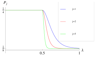
Figure 3: Inverse participation ratio of the Husimi distribution as a function of λ𝜆\lambda for different values of j𝑗j and λc=0.5subscript𝜆𝑐0.5\lambda_{c}=0.5.

Figure 3 shows that Pj(λ)subscript𝑃𝑗𝜆P_{j}(\lambda) tends to a Heaviside-type step function

P(λ)={1/4,ifλ<λc1/8,ifλλc,subscript𝑃𝜆cases14if𝜆subscript𝜆𝑐18if𝜆subscript𝜆𝑐P_{\infty}(\lambda)=\left\{\begin{array}[]{ll}1/{4},&\mathrm{if}\,\lambda<\lambda_{c}\\ {1}/{8},&\mathrm{if}\,\lambda\geq\lambda_{c},\end{array}\right. (41)

which suffers a sudden decrease of 1/4141/4 from normal to superradiant phase, thus indicating a delocalization of ΦΦ\Phi above the critical point λcsubscript𝜆𝑐\lambda_{c}. A similar behavior is displayed by higher moments in the thermodynamic limit

Mj,ν(λ)j{ν2,ifλ<λc21νν2,ifλλc.superscript𝑗subscript𝑀𝑗𝜈𝜆casessuperscript𝜈2if𝜆subscript𝜆𝑐superscript21𝜈superscript𝜈2if𝜆subscript𝜆𝑐M_{j,\nu}(\lambda)\stackrel{{\scriptstyle j\to\infty}}{{\longrightarrow}}\left\{\begin{array}[]{ll}{\nu^{-2}},&\mathrm{if}\,\lambda<\lambda_{c}\\ {2^{1-\nu}\nu^{-2}},&\mathrm{if}\,\lambda\geq\lambda_{c}.\end{array}\right. (42)

The definition of the moments Mj,νsubscript𝑀𝑗𝜈M_{j,\nu} is not restricted to integer values of ν𝜈\nu. Once Mj,νsubscript𝑀𝑗𝜈M_{j,\nu} are known for all integer ν𝜈\nu, there is a unique analytic extension to real ν>0𝜈0\nu>0 (and to the right half complex plane). This analytic extension is possible due to the particular expression of ΦΦ\Phi in therms of Gaussian bells. Using (42), we can easily compute Rényi-Wehrl entropies (20) and, in the limit ν1𝜈1\nu\to 1, the Wehrl entropy (21) in the thermodynamic limit

Wj(λ)j{2,ifλ<λc2+ln(2),ifλλc.superscript𝑗subscript𝑊𝑗𝜆cases2if𝜆subscript𝜆𝑐22if𝜆subscript𝜆𝑐W_{j}(\lambda)\stackrel{{\scriptstyle j\to\infty}}{{\longrightarrow}}\left\{\begin{array}[]{ll}2,&\mathrm{if}\,\lambda<\lambda_{c}\\ 2+\ln(2),&\mathrm{if}\,\lambda\geq\lambda_{c}.\end{array}\right. (43)

This result is in agreement with the (still unproved) Lieb’s conjecture. Indeed, as conjectured by Wehrl Wehrl and proved by Lieb Lieb , any Glauber coherent state |αket𝛼|\alpha\rangle has a minimum Wehrl entropy of 1. In the same paper by Lieb Lieb , it was also conjectured that the extension of Wehrl’s definition of entropy for coherent spin-j𝑗j states will yield a minimum entropy j/(j+1)𝑗𝑗1j/(j+1). For the joined system of radiation field plus atoms we would have Wj(λ)=1+j/(j+1)subscript𝑊𝑗𝜆1𝑗𝑗1W_{j}(\lambda)=1+j/(j+1) in the normal phase (λ<λc𝜆subscript𝜆𝑐\lambda<\lambda_{c}), and therefore, Wj2subscript𝑊𝑗2W_{j}\to 2 in the thermodynamic limit, in agreement with our result.

III.3 Marginals of the Husimi distribution

The explicit expression of the marginal Husimi distributions (22) for our variational ground state ψ𝜓\psi are

Φ1(α1,β1)subscriptΦ1subscript𝛼1subscript𝛽1\displaystyle\Phi_{1}(\alpha_{1},\beta_{1}) =\displaystyle= 1+eαe2+βe2cosh(2(α1αe+β1βe))eα12+β12(1+e2αe2+2βe2),1superscript𝑒superscriptsubscript𝛼𝑒2superscriptsubscript𝛽𝑒22subscript𝛼1subscript𝛼𝑒subscript𝛽1subscript𝛽𝑒superscript𝑒superscriptsubscript𝛼12superscriptsubscript𝛽121superscript𝑒2superscriptsubscript𝛼𝑒22superscriptsubscript𝛽𝑒2\displaystyle\frac{1+e^{\alpha_{e}^{2}+\beta_{e}^{2}}\cosh(2(\alpha_{1}\alpha_{e}+\beta_{1}\beta_{e}))}{e^{\alpha_{1}^{2}+\beta_{1}^{2}}(1+e^{2\alpha_{e}^{2}+2\beta_{e}^{2}})},
Φ2(α2,β2)subscriptΦ2subscript𝛼2subscript𝛽2\displaystyle\Phi_{2}(\alpha_{2},\beta_{2}) =\displaystyle= 1+eαe2βe2cos(2(α2αe+β2βe))eα22+β22(1+e2αe22βe2).1superscript𝑒superscriptsubscript𝛼𝑒2superscriptsubscript𝛽𝑒22subscript𝛼2subscript𝛼𝑒subscript𝛽2subscript𝛽𝑒superscript𝑒superscriptsubscript𝛼22superscriptsubscript𝛽221superscript𝑒2superscriptsubscript𝛼𝑒22superscriptsubscript𝛽𝑒2\displaystyle\frac{1+e^{-\alpha_{e}^{2}-\beta_{e}^{2}}\cos(2(\alpha_{2}\alpha_{e}+\beta_{2}\beta_{e}))}{e^{\alpha_{2}^{2}+\beta_{2}^{2}}(1+e^{-2\alpha_{e}^{2}-2\beta_{e}^{2}})}. (44)

Using the definition (24), we can compute inverse participation ratios for marginal distributions as a function of ζj(λ)eαe2+βe2subscript𝜁𝑗𝜆superscript𝑒superscriptsubscript𝛼𝑒2superscriptsubscript𝛽𝑒2\zeta_{j}(\lambda)\equiv e^{\alpha_{e}^{2}+\beta_{e}^{2}}:

Pj(1)(λ)superscriptsubscript𝑃𝑗1𝜆\displaystyle P_{j}^{(1)}(\lambda) =\displaystyle= 2+4ζj3/2(λ)+ζj2(λ)+ζj4(λ)4(1+ζj2(λ))2,24subscriptsuperscript𝜁32𝑗𝜆subscriptsuperscript𝜁2𝑗𝜆subscriptsuperscript𝜁4𝑗𝜆4superscript1subscriptsuperscript𝜁2𝑗𝜆2\displaystyle\frac{2+4\zeta^{3/2}_{j}(\lambda)+\zeta^{2}_{j}(\lambda)+\zeta^{4}_{j}(\lambda)}{4(1+\zeta^{2}_{j}(\lambda))^{2}},
Pj(2)(λ)superscriptsubscript𝑃𝑗2𝜆\displaystyle P_{j}^{(2)}(\lambda) =\displaystyle= 1+ζj2(λ)+4ζj5/2(λ)+2ζj4(λ)4(1+ζj2(λ))2.1subscriptsuperscript𝜁2𝑗𝜆4subscriptsuperscript𝜁52𝑗𝜆2subscriptsuperscript𝜁4𝑗𝜆4superscript1subscriptsuperscript𝜁2𝑗𝜆2\displaystyle\frac{1+\zeta^{2}_{j}(\lambda)+4\zeta^{5/2}_{j}(\lambda)+2\zeta^{4}_{j}(\lambda)}{4(1+\zeta^{2}_{j}(\lambda))^{2}}. (45)
Refer to caption
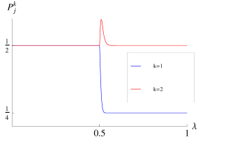
Figure 4: Marginal inverse participation ratios Pj(κ),κ=1,2formulae-sequencesuperscriptsubscript𝑃𝑗𝜅𝜅12P_{j}^{(\kappa)},\kappa=1,2 (position and momentum, resp.) of the Husimi distribution as a function of λ𝜆\lambda for j=10𝑗10j=10 and λc=0.5subscript𝜆𝑐0.5\lambda_{c}=0.5.

Figure 4 shows Pj(κ)(λ)superscriptsubscript𝑃𝑗𝜅𝜆P_{j}^{(\kappa)}(\lambda) for j=10𝑗10j=10, indicating that Pj(1)(λ)superscriptsubscript𝑃𝑗1𝜆P_{j}^{(1)}(\lambda) suffers a sudden decrease from 1/2121/2 to 1/4141/4 across the phase transition, whereas Pj(2)(λ)superscriptsubscript𝑃𝑗2𝜆P_{j}^{(2)}(\lambda) remains constant (the small peak around λc=0.5subscript𝜆𝑐0.5\lambda_{c}=0.5 is perhaps an artifact due to the approximate character of αe,βesubscript𝛼𝑒subscript𝛽𝑒\alpha_{e},\beta_{e} in a neighborhood of λcsubscript𝜆𝑐\lambda_{c}). In general, higher moments of marginal distributions in the thermodynamic limit are given by:

Mj,ν(1)(λ)superscriptsubscript𝑀𝑗𝜈1𝜆\displaystyle M_{j,\nu}^{(1)}(\lambda) jsuperscript𝑗\displaystyle\stackrel{{\scriptstyle j\to\infty}}{{\longrightarrow}} {ν1,ifλ<λc21νν1,ifλλc.,casessuperscript𝜈1if𝜆subscript𝜆𝑐superscript21𝜈superscript𝜈1if𝜆subscript𝜆𝑐\displaystyle\left\{\begin{array}[]{ll}{\nu^{-1}},&\mathrm{if}\,\lambda<\lambda_{c}\\ {2^{1-\nu}\nu^{-1}},&\mathrm{if}\,\lambda\geq\lambda_{c}.\end{array}\right., (48)
Mj,ν(2)(λ)superscriptsubscript𝑀𝑗𝜈2𝜆\displaystyle M_{j,\nu}^{(2)}(\lambda) jsuperscript𝑗\displaystyle\stackrel{{\scriptstyle j\to\infty}}{{\longrightarrow}} ν1,λ,superscript𝜈1for-all𝜆\displaystyle\nu^{-1}\,,\,\,\forall\lambda, (49)

so that, in this limit, we have Mj,ν(λ)=Mj,ν(1)(λ)Mj,ν(2)(λ)subscript𝑀𝑗𝜈𝜆superscriptsubscript𝑀𝑗𝜈1𝜆superscriptsubscript𝑀𝑗𝜈2𝜆M_{j,\nu}(\lambda)=M_{j,\nu}^{(1)}(\lambda)M_{j,\nu}^{(2)}(\lambda). This equality is not true in general for finite j𝑗j and λ>λc𝜆subscript𝜆𝑐\lambda>\lambda_{c}, as can be directly checked for ν=2𝜈2\nu=2 from (40) and (45). Now we see that the entropy excess of ln(2)2\ln(2) comes from the position contribution, since Wehrl entropy in momentum space remains constant:

Wj(1)(λ)j{1,ifλ<λc1+ln(2),ifλλc.superscript𝑗subscriptsuperscript𝑊1𝑗𝜆cases1if𝜆subscript𝜆𝑐12if𝜆subscript𝜆𝑐W^{(1)}_{j}(\lambda)\stackrel{{\scriptstyle j\to\infty}}{{\longrightarrow}}\left\{\begin{array}[]{ll}1,&\mathrm{if}\,\lambda<\lambda_{c}\\ 1+\ln(2),&\mathrm{if}\,\lambda\geq\lambda_{c}.\end{array}\right. (50)
Wj(2)(λ)j1superscript𝑗subscriptsuperscript𝑊2𝑗𝜆1W^{(2)}_{j}(\lambda)\stackrel{{\scriptstyle j\to\infty}}{{\longrightarrow}}1 (51)

In order to connect with (60), we introduce position and momentum operators for the two bosonic modes as in (10). Taking into account the position and momentum representation of an ordinary (canonical) CS (59), the explicit expression of the ground state wave function |αe,βe+subscriptketsubscript𝛼𝑒subscript𝛽𝑒|\alpha_{e},\beta_{e}\rangle_{+} in position (ψ(x,y)=x,y|αe,βe,+𝜓𝑥𝑦inner-product𝑥𝑦subscript𝛼𝑒subscript𝛽𝑒\psi(x,y)=\langle x,y|\alpha_{e},\beta_{e},+\rangle) and momentum (ψ~(px,py)=px,py|αe,βe,+~𝜓subscript𝑝𝑥subscript𝑝𝑦inner-productsubscript𝑝𝑥subscript𝑝𝑦subscript𝛼𝑒subscript𝛽𝑒\tilde{\psi}(p_{x},p_{y})=\langle p_{x},p_{y}|\alpha_{e},\beta_{e},+\rangle) representations can be easily obtained as:

ψ(x,y)𝜓𝑥𝑦\displaystyle\psi(x,y) =\displaystyle= ωω0π𝒩+(αe,βe)𝜔subscript𝜔0𝜋subscript𝒩subscript𝛼𝑒subscript𝛽𝑒\displaystyle\sqrt{\frac{\omega\omega_{0}}{\pi}}{\mathcal{N}}_{+}(\alpha_{e},\beta_{e})
×(e12(ωx2αe)212(ω0y2βe)2\displaystyle\times\left(e^{-\frac{1}{2}{(\sqrt{\omega}\,x-\sqrt{2}\,\alpha_{e})^{2}}-\frac{1}{2}{(\sqrt{\omega_{0}}\,y-\sqrt{2}\,\beta_{e})^{2}}}\right.
+e12(ωx+2αe)212(ω0y+2βe)2),\displaystyle+\left.e^{-\frac{1}{2}{(\sqrt{\omega}\,x+\sqrt{2}\,\alpha_{e})^{2}}-\frac{1}{2}{(\sqrt{\omega_{0}}\,y+\sqrt{2}\,\beta_{e})^{2}}}\right),
ψ~(px,py)~𝜓subscript𝑝𝑥subscript𝑝𝑦\displaystyle\tilde{\psi}(p_{x},p_{y}) =\displaystyle= 2ωω0π𝒩+(αe,βe)2𝜔subscript𝜔0𝜋subscript𝒩subscript𝛼𝑒subscript𝛽𝑒\displaystyle\frac{2}{\sqrt{\omega\omega_{0}\pi}}{\mathcal{N}}_{+}(\alpha_{e},\beta_{e})
×epx22ωpy22ω0cos(2(pxωαe+pyω0βe)),absentsuperscript𝑒superscriptsubscript𝑝𝑥22𝜔superscriptsubscript𝑝𝑦22subscript𝜔02subscript𝑝𝑥𝜔subscript𝛼𝑒subscript𝑝𝑦subscript𝜔0subscript𝛽𝑒\displaystyle\times e^{-\frac{p_{x}^{2}}{2\omega}-\frac{p_{y}^{2}}{2\omega_{0}}}\cos\left(\sqrt{2}(\frac{p_{x}}{\sqrt{\omega}}\alpha_{e}+\frac{p_{y}}{\sqrt{\omega_{0}}}\beta_{e})\right),

where 𝒩+(αe,βe)=(2(1+e2αe22βe2))1/2subscript𝒩subscript𝛼𝑒subscript𝛽𝑒superscript21superscript𝑒2superscriptsubscript𝛼𝑒22superscriptsubscript𝛽𝑒212{\mathcal{N}}_{+}(\alpha_{e},\beta_{e})=\left({2}(1+e^{-2\alpha_{e}^{2}-2\beta_{e}^{2}})\right)^{-1/2} is the typical normalization factor obtained earlier. Note that for λ>λc𝜆subscript𝜆𝑐\lambda>\lambda_{c} the ground-state wave function ψ(x,y)𝜓𝑥𝑦\psi(x,y) splits up into two Gaussian packets centered at antipodal points 2(αe,βe)2subscript𝛼𝑒subscript𝛽𝑒\sqrt{2}(\alpha_{e},\beta_{e}) and 2(αe,βe)2subscript𝛼𝑒subscript𝛽𝑒-\sqrt{2}(\alpha_{e},\beta_{e}) in the xy𝑥𝑦x-y plane. The packets move away from each other for increasing j𝑗j above the critical point λ>λc𝜆subscript𝜆𝑐\lambda>\lambda_{c}. In momentum space, ψ~(px,py)~𝜓subscript𝑝𝑥subscript𝑝𝑦\tilde{\psi}(p_{x},p_{y}) is a Gaussian modulated by a cosine function which oscillates rapidly for high j𝑗j for λ>λc𝜆subscript𝜆𝑐\lambda>\lambda_{c}.

III.4 Zeros of the Husimi distribution and QPT

It is well known that the Husimi density is determined by its zeros through the Weierstrass-Hadamard factorization. It has also been observed that the distribution of zeros differs for classically regular or chaotic systems and can be considered as a quantum indicator of classical chaos (see e.g. Korsch ; monteiro ; 4 ).

Here we shall explore the distribution of zeros of the Husimi density as a fingerprint of QPT in the Dicke model. From (38) we obtain

Ψ(α,z)=02α¯αe+2jln1+z¯ze1z¯ze=iπ(2l+1),l.formulae-sequenceΨ𝛼𝑧02¯𝛼subscript𝛼𝑒2𝑗1¯𝑧subscript𝑧𝑒1¯𝑧subscript𝑧𝑒𝑖𝜋2𝑙1𝑙{\Psi}(\alpha,z)=0\Rightarrow 2\bar{\alpha}\alpha_{e}+2j\ln\frac{1+\bar{z}z_{e}}{1-\bar{z}z_{e}}=i\pi(2l+1),\,l\in\mathbb{Z}. (54)

Instead of this condition, we shall use the approximation (15) and from (39) obtain

Φ(α,β)=02α¯αe+2β¯βe=iπ(2l+1),l,formulae-sequenceΦ𝛼𝛽02¯𝛼subscript𝛼𝑒2¯𝛽subscript𝛽𝑒𝑖𝜋2𝑙1𝑙{\Phi}(\alpha,\beta)=0\Rightarrow 2\bar{\alpha}\alpha_{e}+2\bar{\beta}\beta_{e}=i\pi(2l+1),\,l\in\mathbb{Z}, (55)

which is equivalent to

α1subscript𝛼1\displaystyle\alpha_{1} =\displaystyle= βeαeβ1,subscript𝛽𝑒subscript𝛼𝑒subscript𝛽1\displaystyle-\frac{\beta_{e}}{\alpha_{e}}\beta_{1}, (56)
α2subscript𝛼2\displaystyle\alpha_{2} =\displaystyle= βeαeβ2π2αe(2l+1).subscript𝛽𝑒subscript𝛼𝑒subscript𝛽2𝜋2subscript𝛼𝑒2𝑙1\displaystyle-\frac{\beta_{e}}{\alpha_{e}}\beta_{2}-\frac{\pi}{2\alpha_{e}}(2l+1). (57)

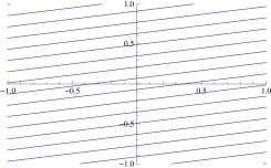
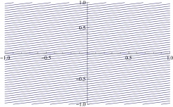
We see that, in the normal phase (αe=0=βesubscript𝛼𝑒0subscript𝛽𝑒\alpha_{e}=0=\beta_{e}) the Husimi distribution Φ(α,β)Φ𝛼𝛽\Phi(\alpha,\beta) has no zeros. In the superradiant phase (λ>λc𝜆subscript𝜆𝑐\lambda>\lambda_{c}) the zeros are localized along straight lines (“dark fringes”) in the α1β1subscript𝛼1subscript𝛽1\alpha_{1}\beta_{1} (position) and α2β2subscript𝛼2subscript𝛽2\alpha_{2}\beta_{2} (momentum) planes. In the momentum plane, the number of dark fringes per cell α2,β2[1,1]subscript𝛼2subscript𝛽211\alpha_{2},\beta_{2}\in[-1,1] grows with λ𝜆\lambda and j𝑗j, as depicted in Figure 5. In the thermodynamic limit j𝑗j\to\infty, zeros densely fill the momentum plane α2β2subscript𝛼2subscript𝛽2\alpha_{2}\beta_{2}.

Refer to caption
Refer to caption
Refer to caption
Refer to caption
Figure 5: Zeros of the Husimi distribution Φ(α,β)Φ𝛼𝛽\Phi(\alpha,\beta) in the cell α2,β2[1,1]subscript𝛼2subscript𝛽211\alpha_{2},\beta_{2}\in[-1,1] of the momentum plane for λ=0.6,j=10formulae-sequence𝜆0.6𝑗10\lambda=0.6,j=10 (top-left), λ=0.6,j=100formulae-sequence𝜆0.6𝑗100\lambda=0.6,j=100 (top-right), λ=10,j=10formulae-sequence𝜆10𝑗10\lambda=10,j=10 (bottom-left) and λ=10,j=100formulae-sequence𝜆10𝑗100\lambda=10,j=100 (bottom-right) for λc=0.5subscript𝜆𝑐0.5\lambda_{c}=0.5.

IV Conclusions

We have found that inverse participation ratios and Rényi-Wehrl entropies of the Husimi distribution provide sharp indicators of a quantum phase transition in the Dicke model. This uncertainty measures detect a delocalization of the Husimi distribution across the critical point λcsubscript𝜆𝑐\lambda_{c} and we have employed them to quantify the phase-space spreading of the states. The advantage of working in phase space is that we can analyze contributions in position and momentum space jointly and separately. Marginal magnitudes in position space turn out to provide sharper indicators of the QPT than in momentum space, where these quantities remain nearly constant. However, zeros of the Husimi distribution exhibit a richer structure in momentum than in position space.

Calculations have been done numerically and through a variational approximation. Numerical calculations are performed by using explicit expressions which have been derived by adopting a truncation of the Holstein-Primakoff representation of the angular momentum operators. The variational approach, in terms of symmetry-adapted coherent states, complements and enriches the analysis providing explicit analytical expressions for the inverse participation ratios and Rényi-Wehrl entropies which remarkably coincide with the numerical results, especially in the thermodynamic limit.

In the superradiant phase, Wehrl’s entropy undergoes an entropy excess (or “subentropy” Jozsa ) of ln(2)2\ln(2). This fact implies that the Husimi distribution splits up into two identical subpackets with negligible overlap in passing from normal to superradiant phase. In general, for s𝑠s identical subpackets with negligible overlap, one would expect an entropy excess of ln(s)𝑠\ln(s). We would like to mention that the Wehrl subentropy (or excess of the Wehrl entropy) has been also used in Mintert as a measure of the degree of mixing for monopartite states or of the degree of entanglement for pure states of bipartite systems. Dicke model is also known to exhibit entanglement between the atoms and the field emaryprl2 ; emarypra and a characterization of it in terms of entropy excesses of this kind would be interesting.

The QPT fingerprints in the Dicke model have also been tracked by exploring the distribution of zeros of the Husimi density within the analytical variational approximation. We have found that the zeros characterize the QPT in this model. Moreover, zeros densely fill the momentum plane in the superradiant phase for the ground state variational approximation in the thermodynamic limit. This subject deserves further attention and should be studied in other models too. For the moment, we have detected a sudden growth of zeros above the critical point λcsubscript𝜆𝑐\lambda_{c} in the Holstein-Primakoff approximation.

Acknowledgments

This work was supported by the Projects: FIS2011-24149 and FIS2011-29813-C02-01 (Spanish MICINN), FQM-165/0207 and FQM219 (Junta de Andalucía).

Appendix A Marginal Husimi distributions as Gaussian smearings

Working on resonance ω=ω0𝜔subscript𝜔0\omega=\omega_{0}, we can introduce a “natural variance” σ2=1/(2ω)superscript𝜎212𝜔\sigma^{2}=1/(2\omega) in the Dicke model by considering the change of coordinates

α1=x2σ,α2=σkx,β1=y2σ,β2=σky,subscript𝛼1𝑥2𝜎subscript𝛼2𝜎subscript𝑘𝑥subscript𝛽1𝑦2𝜎subscript𝛽2𝜎subscript𝑘𝑦\begin{array}[]{ll}\alpha_{1}=\frac{x}{2\sigma},&\alpha_{2}=\sigma k_{x},\\ \beta_{1}=\frac{y}{2\sigma},&\beta_{2}=\sigma k_{y},\end{array} (58)

with 𝐫=(x,y),𝐤=(kx,ky)formulae-sequence𝐫𝑥𝑦𝐤subscript𝑘𝑥subscript𝑘𝑦\mathbf{r}=(x,y),\mathbf{k}=(k_{x},k_{y}) position and momentum vectors. Taking into account the position and momentum representation of an ordinary (canonical) CS Perelomov :

x|αinner-product𝑥𝛼\displaystyle\langle x|\alpha\rangle =\displaystyle= (ω2π)1/4ei2ωα2xe(ωx2α1)2/2,superscriptsuperscript𝜔2𝜋14superscript𝑒𝑖2𝜔subscript𝛼2𝑥superscript𝑒superscript𝜔𝑥2subscript𝛼122\displaystyle\left(\frac{\omega^{2}}{\pi}\right)^{1/4}e^{i\sqrt{2\omega}\,\alpha_{2}x}e^{-{(\sqrt{\omega}\,x-\sqrt{2}\,\alpha_{1})^{2}}/{2}},
k|αinner-product𝑘𝛼\displaystyle\langle k|\alpha\rangle =\displaystyle= (1πω2)1/4ei2ωα1ke(kω2α2)2/2,superscript1𝜋superscript𝜔214superscript𝑒𝑖2𝜔subscript𝛼1𝑘superscript𝑒superscript𝑘𝜔2subscript𝛼222\displaystyle\left(\frac{1}{\pi\omega^{2}}\right)^{1/4}e^{i\sqrt{\frac{2}{\omega}}\,\alpha_{1}k}e^{-{(\frac{k}{\sqrt{\omega}}-\sqrt{2}\,\alpha_{2})^{2}}/{2}}, (59)

one can easily see that marginal distributions (22) can be also obtained as a smearing (convolution product) of the density functions |ψ(𝐫)|2superscript𝜓𝐫2|\psi(\mathbf{r})|^{2} and |ψ~(𝐤)|2superscript~𝜓𝐤2|\tilde{\psi}(\mathbf{k})|^{2} by Gaussians gσ(𝐫)=(2πσ2)1exp(𝐫2/(2σ2))subscript𝑔𝜎𝐫superscript2𝜋superscript𝜎21superscript𝐫22superscript𝜎2g_{\sigma}({\bf r})=(2\pi\sigma^{2})^{-1}\exp{\left(-{{\bf r}^{2}}/({2\sigma^{2}})\right)} and g~σ(𝐤)=4πσ2exp(2σ2𝐤2)subscript~𝑔𝜎𝐤4𝜋superscript𝜎22superscript𝜎2superscript𝐤2\tilde{g}_{\sigma}({\bf k})=4\pi\sigma^{2}\exp{\left(-2\sigma^{2}{{\bf k}^{2}}\right)} as:

ξ(𝐫)𝜉𝐫\displaystyle\xi({\bf r}) =\displaystyle= 𝑑𝐫gσ(𝐫𝐫)|ψ(𝐫)|2differential-dsuperscript𝐫subscript𝑔𝜎𝐫superscript𝐫superscript𝜓superscript𝐫2\displaystyle\int d{\bf r}^{\prime}g_{\sigma}({\bf r}-{\bf r}^{\prime})|\psi({\bf r}^{\prime})|^{2} (60)
ξ~(𝐤)~𝜉𝐤\displaystyle\tilde{\xi}({\bf k}) =\displaystyle= d𝐤(2π)2g~σ(𝐤𝐤)|ψ~(𝐤)|2𝑑superscript𝐤superscript2𝜋2subscript~𝑔𝜎𝐤superscript𝐤superscript~𝜓superscript𝐤2\displaystyle\int\frac{d{\bf k}^{\prime}}{(2\pi)^{2}}\tilde{g}_{\sigma}({\bf k}-{\bf k}^{\prime})|\tilde{\psi}({\bf k}^{\prime})|^{2}

with 𝑑𝐫ξ(𝐫)=1differential-d𝐫𝜉𝐫1\int d{\bf r}\xi({\bf r})=1 and d𝐤(2π)2ξ~(𝐤)=1𝑑𝐤superscript2𝜋2~𝜉𝐤1\int\frac{d{\bf k}}{(2\pi)^{2}}\tilde{\xi}({\bf k})=1. Inverse participation ratios and and Wehrl entropies for these marginal distributions are now written as:

Pjξ=𝑑𝐫ξ2(𝐫),Pjξ~=d𝐤(2π)2ξ~2(𝐤)formulae-sequencesuperscriptsubscript𝑃𝑗𝜉differential-d𝐫superscript𝜉2𝐫superscriptsubscript𝑃𝑗~𝜉𝑑𝐤superscript2𝜋2superscript~𝜉2𝐤P_{j}^{\xi}=\int d{\bf r}\xi^{2}({\bf r}),\quad P_{j}^{\tilde{\xi}}=\int\frac{d{\bf k}}{(2\pi)^{2}}\tilde{\xi}^{2}({\bf k}) (61)
Wjξ=𝑑𝐫ξ(𝐫)lnξ(𝐫),Wjξ~=d𝐤(2π)2ξ~(𝐤)lnξ~(𝐤).formulae-sequencesuperscriptsubscript𝑊𝑗𝜉differential-d𝐫𝜉𝐫𝜉𝐫superscriptsubscript𝑊𝑗~𝜉𝑑𝐤superscript2𝜋2~𝜉𝐤~𝜉𝐤W_{j}^{\xi}=\int d{\bf r}\xi({\bf r})\ln\xi({\bf r}),\quad W_{j}^{\tilde{\xi}}=\int\frac{d{\bf k}}{(2\pi)^{2}}\tilde{\xi}({\bf k})\ln\tilde{\xi}({\bf k}). (62)

More, explicitly, from (11) and (13), marginal Husimi distributions (60) are given in terms of the coefficients cnm(j)superscriptsubscript𝑐𝑛𝑚𝑗c_{nm}^{(j)} as:

ξ(x,y)=n,m,n,mcnm(j)cnm(j)In,n(x)Im+j,m+j(y)𝜉𝑥𝑦subscript𝑛𝑚superscript𝑛superscript𝑚superscriptsubscript𝑐𝑛𝑚𝑗superscriptsubscript𝑐superscript𝑛superscript𝑚𝑗subscript𝐼𝑛superscript𝑛𝑥subscript𝐼𝑚𝑗superscript𝑚𝑗𝑦\xi(x,y)=\sum_{n,m,n^{\prime},m^{\prime}}c_{nm}^{(j)}c_{n^{\prime}m^{\prime}}^{(j)}I_{n,n^{\prime}}(x)I_{m+j,m^{\prime}+j}(y) (63)

and

ξ~(kx,ky)=(2π)2n,m,n,mdnm(j)dnm(j)In,n(px)Im+j,m+j(py)~𝜉subscript𝑘𝑥subscript𝑘𝑦superscript2𝜋2subscript𝑛𝑚superscript𝑛superscript𝑚superscriptsubscript𝑑𝑛𝑚𝑗superscriptsubscript𝑑superscript𝑛superscript𝑚𝑗subscript𝐼𝑛superscript𝑛subscript𝑝𝑥subscript𝐼𝑚𝑗superscript𝑚𝑗subscript𝑝𝑦\tilde{\xi}(k_{x},k_{y})=(2\pi)^{2}\sum_{n,m,n^{\prime},m^{\prime}}d_{nm}^{(j)}d_{n^{\prime}m^{\prime}}^{(j)}I_{n,n^{\prime}}(p_{x})I_{m+j,m^{\prime}+j}(p_{y}) (64)

with dnm(j)(i)n+m+jcnm(j)superscriptsubscript𝑑𝑛𝑚𝑗superscript𝑖𝑛𝑚𝑗superscriptsubscript𝑐𝑛𝑚𝑗d_{nm}^{(j)}\equiv(-i)^{n+m+j}c_{nm}^{(j)} and

In,n(x)=Aαn!n!(1α22)n+nex21+2σ2subscript𝐼𝑛superscript𝑛𝑥𝐴𝛼𝑛superscript𝑛superscript1superscript𝛼22𝑛superscript𝑛superscript𝑒superscript𝑥212superscript𝜎2\displaystyle I_{n,n^{\prime}}(x)=A\alpha\sqrt{n!n^{\prime}!\left(\frac{1-\alpha^{2}}{2}\right)^{n+n^{\prime}}}e^{\frac{-x^{2}}{1+2\sigma^{2}}} (65)
×k=0μB(n,n,k)(21α2)kHn+n2k(αs(1α2)1/2)\displaystyle\times\sum_{k=0}^{\mu}B(n,n^{\prime},k)\left(\frac{2}{1-\alpha^{2}}\right)^{k}H_{n+n^{\prime}-2k}\left(\frac{\alpha s}{(1-\alpha^{2})^{1/2}}\right)

with μ=min{n,n}𝜇𝑛superscript𝑛\mu=\min\left\{n,n^{\prime}\right\}, A=(2πσ2)1/2𝐴superscript2𝜋superscript𝜎212A=(2\pi\sigma^{2})^{-1/2}, B(n,n,k)=1(k!)(nk)!(nk)!𝐵𝑛superscript𝑛𝑘1𝑘𝑛𝑘superscript𝑛𝑘B(n,n^{\prime},k)=\frac{1}{(k!)(n-k)!(n^{\prime}-k)!}, α=2σ22σ2+1𝛼2superscript𝜎22superscript𝜎21\alpha=\sqrt{\frac{2\sigma^{2}}{2\sigma^{2}+1}} and s=xσ2(1+2σ2)𝑠𝑥𝜎212superscript𝜎2s=\frac{x}{\sigma\sqrt{2(1+2\sigma^{2})}}. Relations between marginal inverse participation ratios and Wehrl entropies in both cases can be straightforwardly obtained: Pjξ=π1Pj(1)superscriptsubscript𝑃𝑗𝜉superscript𝜋1superscriptsubscript𝑃𝑗1P_{j}^{\xi}=\pi^{-1}P_{j}^{(1)} and Pjξ~=πPj(2)superscriptsubscript𝑃𝑗~𝜉𝜋superscriptsubscript𝑃𝑗2P_{j}^{\tilde{\xi}}=\pi P_{j}^{(2)} and Wjξ=Wj(1)+ln(2π)superscriptsubscript𝑊𝑗𝜉superscriptsubscript𝑊𝑗12𝜋W_{j}^{\xi}=W_{j}^{(1)}+\ln(2\pi) and Wjξ~=Wj(2)ln(2π)superscriptsubscript𝑊𝑗~𝜉superscriptsubscript𝑊𝑗22𝜋W_{j}^{\tilde{\xi}}=W_{j}^{(2)}-\ln(2\pi).

References

  • (1) S. Sachdev, Quantum Phase Transitions, Cambridge University Press (2000).
  • (2) C. C. Gerry and P. L. Knight, Introductory Quantum Optics, Cambridge University Press (2005).
  • (3) C. Aulbach, A. Wobst, G.-L. Ingold, P. Hanggi and I. Varga, New J. of Physics 6, 70 (2004).
  • (4) P. A. Dando and T. S. Monteiro, J. Phys. B. 27, 2681, (1994).
  • (5) D. Weinmann , S. Kohler, G-L. Ingold and P. H nggi, Ann. Phys. (Lpz) 8 SI277 (1999).
  • (6) H. J. Korsch, C. Müller and H. Wiescher, J. Phys. A 30, L677 (1997).
  • (7) P. Leboeuf and A. Voros, J. Phys. A 23, 1765 (1990).
  • (8) P. A. Dando, and T. S. Monteiro, J. Phys. B 27, 2681 (1994).
  • (9) F. Mintert and K. Zyczkowski, Phys. Rev. A 69, 022317 (2004).
  • (10) E. Romera and Á. Nagy, Phys. Lett. A 375 3066 (2011).
  • (11) E. Romera, K. Sen and Á. Nagy, J.Stat. Mech. doi:10.1088/1742-5468/2011/09/P09016
  • (12) E. Romera, M. Calixto and Á. Nagy, Europhys. Lett. 97, 20011 (2012).
  • (13) Á. Nagy and E. Romera, Physica A doi: 10.1016/j.physa.2012.02.024 (2012).
  • (14) M. Calixto, Á. Nagy, I. Paraleda and E. Romera (submitted, 2012).
  • (15) N. Lambert, C. Emary, and T. Brandes, Phys. Rev. Lett. 92, 073602 (2004).
  • (16) N. Lambert, C. Emary, and T. Brandes, Phys. Rev.A 71, 053804 (2005).
  • (17) T. Brandes, Phys. Rep. 408, 315 (2005).
  • (18) A. Perelomov, Generalized Coherent States and Their Applications, Springer-Verlag (1986).
  • (19) T. Holstein and H. Primakoff, Phys. Rev. 58, 1098 (1940).
  • (20) C. Emary and T. Brandes, Phys. Rev. E 67, 066203 (2003).
  • (21) M. A. Bastarrachea-Magnani, J. G. Hirsch Numerical solutions of the Dicke Hamiltonian, arxiv:1108.0703 (2011)
  • (22) J.M. Radcliffe, J. Phys. A 4, 313 (1971).
  • (23) O. Castaños, E. Nahmad-Achar, R. López-Peña and J. G. Hirsch, Phys. Rev. A 83, 051601 (2011).
  • (24) O. Castaños, E. Nahmad-Achar, R. López-Peña, and J. G. Hirsch, Phys. Rev. A, 84 013819 (2011).
  • (25) A. Wehrl, Rep. Math. Phys. 16, 353 (1979)
  • (26) E.H. Lieb, Commun. Math. Phys. 62, 35 (1978)
  • (27) R. Jozsa, D. Robb and W.K. Wootters, Phys. Rev. A 49, 668 (1994).