Enabling Incremental Query Re-Optimization

Abstract

As declarative query processing techniques expand in scope — to the Web, data streams, network routers, and cloud platforms — there is an increasing need for adaptive query processing techniques that can re-plan in the presence of failures or unanticipated performance changes. A status update on the data distributions or the compute nodes may have significant repercussions on the choice of which query plan should be running. Ideally, new system architectures would be able to make cost-based decisions about reallocating work, migrating data, etc., and react quickly as real-time status information becomes available. Existing cost-based query optimizers are not incremental in nature, and must be run “from scratch” upon each status or cost update. Hence, they generally result in adaptive schemes that can only react slowly to updates.

An open question has been whether it is possible to build a cost-based re-optimization architecture for adaptive query processing in a streaming or repeated query execution environment, e.g., by incrementally updating optimizer state given new cost information. We show that this can be achieved beneficially, especially for stream processing workloads. Our techniques build upon the recently proposed approach of formulating query plan enumeration as a set of recursive datalog queries; we develop a variety of novel optimization approaches to ensure effective pruning in both static and incremental cases. We implement our solution within an existing research query processing system, and show that it effectively supports cost-based initial optimization as well as frequent adaptivity.

1 Introduction

The problem of supporting rapid adaptation to runtime conditions during query processing — adaptive query processing aqp-survey — is of increasing importance in today’s data processing environments. Consider declarative cloud data processing systems boom-analytics ; asterix ; DBLP:journals/pvldb/MelnikGLRSTV10 and data stream processing aurora ; stanford-stream ; telegraphcq platforms, where data properties and the status of cluster compute nodes may be constantly changing. Here it is very difficult to effectively choose a good plan for query execution: data statistics may be unavailable or highly variable; cost parameters may change due to resource contention or machine failures; and in fact a combination of query plans might perform better than any single plan. Similarly, in conventional DBMSs there may be a need to perform self-tuning so the performance of a query or set of queries can be improved db2-mqreopt .

To this point, query optimization techniques in adaptive query processing systems fall into three general classes: (1) operator-specific techniques that can adapt the order of evaluation for filtering operators stanford-aqp ; (2) eddies DBLP:conf/sigmod/AvnurH00 ; stairs and related flow heuristics, which are highly adaptive but also continuously devote resources to exploring all plans and require fully pipelined execution; (3) approaches that use a cost-based query re-optimizer to re-estimate plan costs and determine whether the system should change plans DBLP:conf/sigmod/KabraD98 ; db2-mqreopt ; tukwila-04 ; cape-04 . Of these, the last is the most flexible, e.g., in that it supports complex query operators like aggregation, as well as expensive adaptations like data repartitioning across a cluster. Perhaps most importantly, a cost-based engine allows the system to spend the majority of its resources on query execution once the various cost parameters have been properly calibrated. Put another way, it can be applied to highly complex plans and has the potential to provide significant benefit if a cost estimation error was made, but it should incur little overhead if a good plan was chosen. Unfortunately, to this point cost-based techniques have not been able to live up to their potential, because the cost-based re-optimization step has been too expensive to perform frequently.

Our goal in this paper is to explore whether incremental techniques for re-optimization can be developed, where an optimizer would only re-explore query plans whose costs were affected by an updated cardinality or cost value; and whether such incremental techniques could be used to facilitate more efficient adaptivity.

Target Domains.

Our long-term goal is to develop adaptive techniques for complex OLAP-style queries (which contain operators not amenable to the use of eddies) being executed across a data-partitioned cluster, as in boom-analytics ; asterix . However, in this paper we focus on developing incremental re-optimization techniques that we evaluate within a single-node (local) query engine, in two main contexts. (1) We address the problem of adaptive query processing in data stream management systems where data may be bursty, and its distributions may vary over time — meaning that different query plans may be preferred over different segments. Here it is vital to optimize frequently based on recent data distribution and cost information, ideally as rapidly as possible. (2) We address query re-optimization in traditional OLAP settings when the same query (or highly similar queries) gets executed frequently, as in a prepared statement. Here we may wish to re-optimize the plan after each iteration, given increasingly accurate information about costs, and we would like this optimization to have minimal overhead.

Approach and Contributions.

The main contribution of this paper is to show for the first time how an incremental re-optimizer can be developed, and how it can be useful in adaptive query processing scenarios matching the application domains cited above. Our incremental re-optimizer implements the basic capabilities of a modern database query optimizer, and could easily be extended to support other more advanced features; our main goal is to show that an incremental optimizer following our model can be competitive with a standard optimizer implementation for initial optimization, and significantly faster for repeated optimization. Moreover, in contrast to randomized or heuristics-based optimization methods, we still guarantee the discovery of the best plan according to the cost model. Since our work is oriented towards adaptive query processing, we evaluate the system in a variety of settings in conjunction with a basic pipelined query engine for stream and stored data.

We implement the approach using a novel approach, which is based on the observation that query optimization is essentially a recursive process involving the derivation and subsequent pruning of state (namely, alternative plans and their costs). If one is to build an incremental re-optimizer, this requires preservation of state (i.e., the optimizer memoization table) across optimization runs — but moreover, it must be possible to determine what plans have been pruned from this state, and to re-derive such alternatives and test whether they are now viable.

One way to achieve such “re-pruning” capabilities is to carefully define a semantics for how state needs to be tracked and recomputed in an optimizer. However, we observe that this task of “re-pruning” in response to updated information looks remarkably similar to the database problem of view maintenance through aggregation springerlink:10.1007/BFb0014149 and recursion as studied in the database literature gms93-dred . In fact, recent work evita-raced has shown that query optimization can itself be captured in recursive datalog. Thus, rather than inventing a custom semantics for incrementally maintaining state within a query optimizer, we instead adopt the approach of developing an incremental re-optimizer expressed declaratively.

More precisely, we express the optimizer as a recursive datalog program consisting of a set of rules, and leverage the existing database query processor to actually execute the declarative program. In essence, this is optimizing a query optimizer using a query processor. Our implementation approaches the performance of conventional procedural optimizers for reasonably-sized queries. Our implementation recovers the initial overhead during subsequent re-optimizations by leveraging incremental view maintenance gms93-dred ; recursive-views techniques. It only recomputes portions of the search space and cost estimates that might be affected by the cost updates. Frequently, this is only a small portion of the overall search space, and hence we often see order-of-magnitude performance benefits.

Our approach achieves pruning levels that rival or best bottom-up (as in System-R systemR ) and top-down (as in Volcano DBLP:journals/debu/Graefe95a ; volcano ) plan enumerations with branch-and-bound pruning. We develop a variety of novel incremental and recursive optimization techniques to capture the kinds of pruning used in a conventional optimizer, and more importantly, to generalize them to the incremental case. Our techniques are of broader interest to incremental evaluation of recursive queries as well. Empirically, we see updates on only a small portion of the overall search space, and hence we often see order-of-magnitude performance benefits of incremental re-optimization. We also show that our re-optimizer fits nicely into a complete adaptive query processing system, and measure both the performance and quality, the latter demonstrated well in the yielded query plans, of our incremental re-optimization techniques on the Linear Road stream benchmark. We make the following contributions:

• The first query optimizer that prunes yet supports incremental re-optimization.

• A rule-based, declarative approach to query (re)optimization. Our implementation decouples plan enumerations and cost estimations, relaxing traditional restrictions on search order and pruning.

• Novel strategies to prune the state of an executing recursive query, such as a declarative optimizer: aggregate selection with tuple source suppression; reference counting; and recursive bounding.

• A formulation of query re-optimization as an incremental view maintenance problem, for which we develop novel algorithms.

• An implementation over a query engine developed for recursive stream processing recursive-views , with a comprehensive evaluation of performance against alternative approaches, over a diverse workload.

• Demonstration that incremental re-optimization can be incorporated to good benefit in existing cost-based adaptive query processing techniques tukwila-04 ; cape-04 .

2 Declarative Query Optimization

Our goal is to develop infrastructure to adapt an optimizer to support efficient, incrementally maintainable state, and incremental pruning. Our focus is on developing techniques for incremental state management for the recursively computed plan costs in the query optimizer, in response to updates to query plan cost information. Incremental update propagation is a very well-studied problem for recursive datalog queries, with a clean semantics and many efficient implementations. Prior work has also demonstrated the feasibility of a datalog-based query optimizer evita-raced . Hence, rather than re-inventing incremental recomputation techniques we have built our optimizer as a series of recursive rules in datalog, executed in the query engine that already exists in the DBMS. (We could have further extended to Prolog, but our goal was clean state management rather than a purely declarative implementation. Other alternatives like constraint programming or planning languages do not support incremental maintenance.)

In contrast to work such as evita-raced , our focus is not on formulating every aspect of query optimization in datalog, but rather on formulating those aspects relating to state management and pruning as datalog rules — so we can use incremental view maintenance (delta rules) and sideways information passing techniques, respectively. Other optimizer features that are not reliant on state that changes at runtime, such as cardinality estimation, breaking expressions into subexpressions, etc., are specified as built-in auxiliary functions. As a result, we specify an entire optimizer in only three stages and 10 rules (dataflow is illustrated in Figure 1).

Plan enumeration ($\mathsf{SearchSpace}$).

Searching the space of possible plans has two aspects. In the logical phase, the original query is recursively broken down into a full set of alternative relational algebra subexpressions. The decomposition is naturally a “top-down” type of recursion: it starts from the original query expression, which it breaks down into subexpressions, and so on. The physical phase takes as input a query expression from the logical phase, and creates physical plans by enumerating the set of possible physical operators that satisfy any constraints on the output properties volcano or “interesting orders” systemR (e.g., the data must be sorted by a particular attribute). Without physical properties, the extension from logical plans to physical plans can be computed either top-down or bottom-up; however, the properties are more efficiently computed in goal-directed (top-down) manner.

Cost estimation ($\mathsf{PlanCost}$).

This phase determines the cost for each physical plan in the search space, by recursively merging the statistics and cost estimates of a plan’s subplans. It is naturally a bottom-up type of recursion, as the plan subexpressions must already have been cost-estimated before the plan itself. Here we can encode in a table the mapping from a plan to its cost.

Plan selection ($\mathsf{BestPlan}$).

As costs are estimated, the program produces the plan that incurs the lowest estimated cost.

In our declarative approach to query optimization, we treat optimizer state as data, use rules to specify what a query optimizer is, and leverage a database query processor to actually perform the computation. Figure 1 shows a (simplified) query plan for the datalog rules. As we can see, the declarative program is by nature recursive, and is broken into the three stages mentioned before (with Fixpoint operators between stages). Starting from the bottom of the figure, plan enumeration recursively generates a $\mathsf{SearchSpace}$ table containing plan specifications, by decomposing the query and enumerating possible output properties; enumerated plans are then fed into the plan estimation component, $\mathsf{PlanCost}$, which computes a cost for each plan, by building from leaf to complex expressions; plan selection computes a $\mathsf{BestCost}$ and $\mathsf{BestPlan}$ entry for each query expression and output property, by aggregating across the $\mathsf{PlanCost}$ entries.

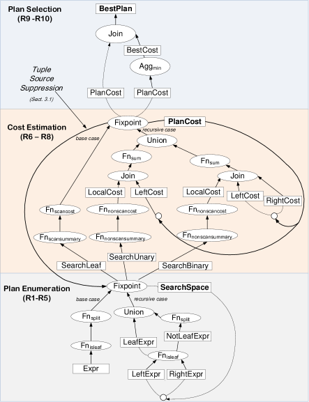
Figure 1: Query plan of our declarative query optimizer. Operators are in ellipses; views are in rectangles. Plan enumeration ($\mathsf{SearchSpace}$) consists of 5 rules, cost estimation ($\mathsf{PlanCost}$) 3 rules, and plan selection ($\mathsf{BestPlan}$) 2 rules. See Appendix.

Example 1

As our driving example, consider a simplified TPC-H Query 3 with its aggregates and functions removed, called Q3S.

⬇

SELECT L_orderkey, O_orderdate, O_shippriority

FROM Customer C, Orders O, Lineitem L

WHERE C_mktsegment = ’MACHINERY’ and C_custkey = O_custkey and O_orderkey = L_orderkey and O_orderdate < ’1995-03-15’ and L_shipdate > ’1995-03-15’

2.1 Plan Enumeration

Plan enumeration takes as input the original query expression as $\mathsf{Expr}$, and then generates as output the set of alternative plans. As with many optimizers, it is divided into two levels:

Logical search space.

The logical plan search space contains all the logical plans that correspond to subexpressions of the original query expression up to any logically equivalent transformations (e.g., commutativity and associativity of join operators). In traditional query optimizers such as Volcano volcano , a data structure called an and-or-graph is maintained to represent the logical plan search space. Bottom-up dynamic programming optimizers do not need to physically store this graph but it is still conceptually relevant.

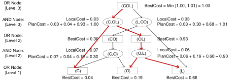
Figure 2: The and-or-graph for Q3S. Red edges denote the best plan. Rectangles and ovals denote “OR” and “AND” nodes respectively. Each “OR” node is labeled with its $\mathsf{BestCost}$ and each “AND” node is labeled with its $\mathsf{LocalCost}$ and $\mathsf{PlanCost}$.

Example 2

Figure 2 shows an example and-or-graph for Q3S, which describes a set of alternative subplans and subplan choices using interleaved levels. “AND” nodes represent alternative subplans (typically with join operator roots) and the “OR” nodes represent decision points where the cheapest AND-node was chosen.

In our implementation, we capture each of the nodes in a table called $\mathsf{SearchSpace}$. In fact, as we discuss next, we supplement this information with further information about the output properties and physical plan. (We explain why we combine the results from both stages in Section 2.3.)

Physical search space.

The physical search space extends the logical one in that it enumerates all the physical operators for each algebraic logical operator. For example, in our figure above, each “AND” node denotes a logical join operator, but it may have multiple physical implementations such as pipelined-hash, indexed nested-loops, or sort-merge join. If the physical implementation is not symmetric, exchanging the left and right child would become a different physical plan. A physical plan has not only a root physical operator, but also a set of physical properties over the data that it maintains or produces; if we desire a set of output properties, this may constrain the physical properties of the plan’s inputs.

*Expr	*Prop	*Index	LogOp	*PhyOp	lExpr	lProp	rExpr	rProp
(COL)	–	1	join	sort-merge	(C)	C_custkey order	(OL)	O_custkey order
(COL)	–	2	join	indexed nested-loop	(L)	index on L_orderkey	(CO)	–
(OL)	O_custkey order	1	join	pipelined-hash	(O)	–	(L)	–
(CO)	–	1	join	pipelined-hash	(C)	–	(O)	–
(CO)	–	1	join	sort-merge	(C)	–	(O)	–
(O)	O_custkey order	–	scan	local scan	–	–	–	–
(L)	index on L_orderkey	–	scan	index scan	–	–	–	–
(C)	C_custkey order	–	scan	local scan	–	–	–	–

Table 1: A simplified $\mathsf{SearchSpace}$ relation encoding the and-or-graph for Q3S’s search space. Primary keys are denoted by *.

Example 3

Table 1 shows the $\mathsf{Search\-Space}$ content for a subset of Figure 2. The AND logical operators are either joins (with 2 child expressions), or tablescans (with selection predicates applied). Each expression $\mathsf{Expr}$ may have multiple $\mathsf{\mathit{Index}}$ed alternatives. $\mathsf{\mathit{Prop}}$ and $\mathsf{\mathit{PhyOp}}$ represent the physical properties of a plan and its root physical operator, respectively.

For instance, expression $\mathsf{SearchSpace}$$(COL)$ has encodes an “OR” node with two alternatives the first “AND” (join) child is $\mathsf{SearchSpace}$$(C,OL)$ and the second is $\mathsf{SearchSpace}$$(L,CO)$. For the first $\mathsf{SearchSpace}$ tuple, the left expression is $C$ and the right expression is $OL$. The tuple indicates a Sort-Merge join, whose left and right inputs’ physical properties require a sort order based on $\mathsf{\mathit{C\_custkey}}$ and $\mathsf{\mathit{O\_custkey}}$, respectively. The second alternative uses an Indexed Nested-Loop Join as its physical operator. The left expression refers to the inner join relation indexed on $\mathsf{\mathit{L\_orderkey}}$, while there are no ordering restrictions on the right expression.

Our datalog-based optimizer enumerates both spaces in the same recursive query (see bottom of Figure 1). Given an expression, the $\mathsf{Fn_{split}}$ function enumerates all the algebraically equivalent rewritings for the given expression, as well as the possible physical operators and their interesting orders. Fixpoint is reached when $\mathsf{Expr}$ has been decomposed down to leaf-level scan operations over a base relation (checked using the $\mathsf{Fn_{isleaf}}$ function).

2.2 Cost Estimation and Plan Selection

The cost estimation component computes an estimated cost for every physical plan. Given the $\mathsf{SearchSpace}$ tuples generated in the plan enumeration phase, three datalog rules (R6 - R8) are used to compute $\mathsf{PlanCost}$ (corresponding to a more detailed version of the “AND” nodes in Figure 2, with physical operators considered and all costs enumerated), and two additional rules (R9 - R10) select the $\mathsf{BestPlan}$ (corresponding to an “OR” node). Cost estimates are recursively computed by summing up the children costs and operation costs. The computed sum for each physical plan is stored in $\mathsf{PlanCost}$.

In addition to the search space, cost estimation requires a set of summaries (statistics) on the input relations and indexes, e.g., cardinality of a (indexed) relation, selectivity of operators, data distribution, etc. These summaries are computed using functions $\mathsf{Fn_{scansummary}}$ and $\mathsf{Fn_{nonscansummary}}$. The former computes the leaf level summaries over base tables, and the latter computes the output summaries of an operator based on input summaries. Given the statistics, the cost of a plan can be computed by combining factors such as CPU, I/O, bandwidth and energy into a single cost metric. We compute the cost of each physical operator using functions $\mathsf{Fn_{scancost}}$ and $\mathsf{Fn_{nonscancost}}$ respectively.

Given the above functions, cost estimation becomes a recursive computation that sums up the cost of children expressions and the root cost, to finally compute a cost for the entire query plan. At each step, $\mathsf{Fn_{sum}}$ is used to sum up the $\mathsf{PlanCost}$ of its child plans with $\mathsf{LocalCost}$. The particular form of the operation depends on whether the plan root is a leaf node, a unary or a binary operator.

Example 4

To illustrate the process of cost estimation, we revisit Figure 2, which shows a simplified logical search space (omitting physical operators and properties) for our simplified TPC-H Q3S. For every “AND” node, we compute the plan cost by summing up the cost of the join operator, with the best costs of computing its two inputs (e.g., the level 2 “AND” node $(C,O)$ sums up its local cost 0.07, its left best cost 0.04, and its right best cost 0.19, and gets its plan cost 0.30). For every “OR” node, we determine the alternative with minimum cost among its “AND” node children (e.g., the level 3 “OR” node $(COL)$ computes a minimum over its two input plan costs 1.00 and 1.01, and gets its best cost 1.00). After the best cost is computed for the root “OR” node in the graph, the optimization process is done, and an optimal plan tree is chosen.

Once the $\mathsf{PlanCost}$ for every “AND” node are generated, the final two rules compute the $\mathsf{BestCost}$ for every “OR” node by computing a min aggregate over $\mathsf{PlanCost}$ of its alternative “AND” node derivations, and output the $\mathsf{BestPlan}$ for each “AND” node by computing a join between $\mathsf{BestCost}$ and $\mathsf{PlanCost}$.

2.3 Execution Strategy

Given a query optimizer specified in datalog, the natural question is how to actually execute it. We seek to be general enough to incorporate typical features of existing query optimizers, to rival their performance and flexibility, and to only develop implementation techniques that generalize. We adopt two strategies:

Merging of logical and physical plan enumeration.

The logical and physical plan enumeration phases are closely related, and in general one can think of the physical plan as an elaboration of the logical one. As both logical and physical enumeration are top-down types of recursion, and as there is no pruning information from the physical stage that should be propagated back to the logical one, we can merge the logical and physical enumeration stages into a single recursive query.

As we enumerate each logical subexpression, we simultaneously join with the table representing the possible physical operators that can implement it. This generates the entire set of possible physical query plans. To make it more efficient to generate multiple physical plans from a single logical expression, we use caching to memoize the results of $\mathsf{Fn_{nonscansummary}}$ and $\mathsf{Fn_{split}}$.

Decoupling of cost estimation and plan enumeration.

Cost estimation requires bottom-up evaluation: a cost estimate can only be obtained once cost estimates and statistics are obtained from child expressions. The enumeration stage naturally produces expressions in the order from parent to child, yet estimation must be done from child to parent. We decouple the execution order among plan enumeration and cost estimation, making the connections between these two components flexible. For example, some cost estimates may happen before all related plans have been enumerated. Cost estimates may even be used to prune portions of the plan enumeration space (and hence also further prune cost estimation itself) in an opportunistic way.

In subsequent sections, we develop techniques to prune and maintain the optimizer state that has no constraints on enumeration order, search order or pruning frequency. Our approach relaxes the traditional restrictions on the search order and pruning techniques in either Volcano’s volcano top-down traversal or System R’s systemR ’s bottom-up dynamic programming approaches. For example, a top-down search may have a depth-first, breadth-first or another order.

We leverage a pipelined push-based query processor to execute the rules in an incremental fashion, which simultaneously explores many expressions. We pipeline the results of plan enumeration to the cost estimation stage without synchronization or blocking. All of our techniques extend naturally to a distributed or parallel setting, which we hope to study in future work.

3 Achieving Pruning

In this section, we describe how we can incorporate pruning of the search space into pipelined execution of our query optimizer. To achieve this, we use techniques based on the idea of sideways information passing, in which the computation of one portion of the query plan may be made more efficient by filtering against information computed elsewhere, but not connected directly by pipelined dataflow. Specifically, we incorporate the technique of aggregate selection sudarshan91aggregation from the deductive database literature, which we briefly review; we extend it to perform further pruning; and we develop two new techniques for recursive queries that enable tracking of dependencies and computation of bounds. Beyond query optimization, our techniques are broadly useful in the evaluation of recursive datalog queries. In the next section we develop novel techniques to make these strategies incrementally maintainable.

Section 3.1 reviews aggregate selection, which removes non-viable plans from the optimizer state if they are not cost-effective, and shows how we can use it to achieve the similar effects to dynamic programming in System-R. There we also introduce a novel technique called tuple source suppression. Then in the remainder of the section we show how to introduce two familiar notions into datalog execution: namely, reference counting that enables us to removes plan subexpressions once all of their parent expressions have been pruned (Section 3.2), and recursive bounding, which lets the datalog engine incorporate branch-and-bound pruning as in a typical Volcano-style top-down query optimizer (Section 3.3). Our solutions are valid for any execution order, take full advantage of the parallel exploration provided by pipelining, and are extensible to parallel or distributed architectures.

3.1 Pruning Suboptimal Plan Expressions

Dating back to System-R systemR , every modern query optimizer uses dynamic programming techniques (although some via memoization volcano ). Dynamic programming is based on the principle of optimality, i.e. an optimal plan can be decomposed into sub-plans that must themselves be optimal solutions. This property is vital to optimizer performance, because the same subexpression may appear repeatedly in many parent expressions. Formally:

Proposition 5

Given a query expression $E$ and property $p$, consider a plan tree $T\langle E,p\rangle$ that evaluates $E$ with output property $p$. For this and other propositions, we assume that plans have distinct costs. Here one such $T$ will have the minimum cost: call that $T_{OPT}$. Suppose $E^{s}$ is a subexpression of $E$, and consider a plan tree $T^{s}\langle E^{s},p^{s}\rangle$ that evaluates $E^{s}$ with output property $p^{s}$. Again one such $T^{s}$ will have the minimum cost: call that $T^{s}_{OPT}$. If $T^{s}$ is not $T^{s}_{OPT}$, then $T^{s}$ must not be the subtree of $T_{OPT}$.

This proposition ensures that we can safely discard suboptimal subplans without affecting the final optimal plan. Consider the and-or-graph of the example query Q3S (Figure 2). The red (bolded) subtree is the optimal plan for the root expression $(COL)$. The subplan of the level 3 “AND” node $(L,CO)$ has suboptimal cost 1.00. If there exists a super-expression containing $(COL)$, then the only viable subplan is the one marked in the figure. State for any alternative subplan for $(COL$) may be pruned from $\mathsf{SearchSpace}$ and $\mathsf{PlanCost}$. We achieve pruning over both relations as follows.

Pruning $\mathsf{PlanCost}$ via aggregate selection.

Refer back to Figure 1: each $\mathsf{BestCost}$ tuple encodes the minimum cost for a given query expression-property pair, over all the plans associated with this pair in $\mathsf{PlanCost}$. To avoid enumerating unnecessary $\mathsf{PlanCost}$ tuples, one can wait until the $\mathsf{BestCost}$ of subplans are obtained before computing a $\mathsf{PlanCost}$ for a root plan. This is how System R-style dynamic programming works. However, this approach constrains the order of evaluation.

We instead extend a logic programming optimization technique called aggregate selection sudarshan91aggregation , to achieve dynamic programming-like benefits for any arbitrary order of implementation. In aggregate selection, we “push down” a selection predicate into the input of an aggregate, such that we can prune results that exceed the current minimum value or are below the current maximum value. In our case (as shown in the middle box of Figure 1), the current best-known cost for any equivalent query expression-property pair is maintained within our Fixpoint operator (which also performs the non-blocked min aggregation). We only propagate a newly generated $\mathsf{PlanCost}$ tuple if its cost is smaller than the current minimum. This does not affect the computation of $\mathsf{BestCost}$, which still outputs the minimum cost for each expression-property pair. Since pruning bounds are updated upon every newly generated tuple, there is no restriction on evaluation order. As with pruning strategies used in Volcano-style optimizers, the amount of state pruned varies depending on the order of exploration: the sooner a min-cost plan is encountered, the more effective the pruning is.

Pruning $\mathsf{SearchSpace}$ via tuple source suppression.

Enumeration of the search space will generally happen in parallel with enumeration of plans. Thus, as we prune tuples from $\mathsf{PlanCost}$, we may be able to remove related tuples (e.g., representing subexpressions) from $\mathsf{SearchSpace}$, possibly preventing enumeration of their subexpressions and/or costs. We achieve such pruning through tuple source suppression, along the arcs indicated in Figure 1. Any $\mathsf{PlanCost}$ tuples pruned by aggregate selection should also trigger cascading deletions to the source tuples by which they were derived from the $\mathsf{SearchSpace}$ relation. To achieve this, since $\mathsf{PlanCost}$ contains a superset of the attributes in $\mathsf{SearchSpace}$, we simply project out the $\mathsf{cost}$ field and propagate a deletion to the corresponding $\mathsf{SearchSpace}$ tuple.

3.2 Pruning Unused Plan Subexpressions

The techniques described in the previous section remove suboptimal plans for specific expression-property pairs. However, ultimately some optimal plans for certain expressions may be unused in the final query execution plan. Consider in Figure 2 the level 2 “AND” node $(C,O)$: this node is not in the final plan because its “OR” node parent expression $(CO)$ does not appear in the final result. In turn, this is because $(CO)$’s parent “AND” nodes (in this example, just a single plan $(L,CO)$) do not contribute to the final plan. Intuitively, we may prune an “AND” node if all of its parent “AND” nodes (through only one connecting “OR” node) have been pruned.

We would like to remove such plans once they are discovered to not appear in the final optimal plan, which requires a form of reference counting within the datalog engine executing the optimizer. To achieve this, every tuple in $\mathsf{SearchSpace}$ is annotated with a count. This count represents the number of parent plans still present in the $\mathsf{SearchSpace}$. For example, in Table 1, the plan entry of $O\Join L$ has reference count of 1, because it only has one parent plan, which is $C\Join OL$; on the other hand, the plan entry of $(O)$ has reference count of 2, because it has two parent plans, which are $O\Join L$ and $C\Join O$. Below is a proposition about reference counting:

Proposition 6

Given a query expression $E$ with output property $p$: let $T^{s}$ be a plan tree for $E$’s subexpression $E^{s}$ with property $p^{s}$. If $T^{s}$ has reference count of zero, then $T^{s}$ must not be a subtree of the optimal plan tree for the query $E$ with property $p$.

The proposition ensures that a plan with a reference count of zero can be safely deleted. Note that a deleted plan may make more reference counts to drop to zero, hence the deletion process may be recursive. Our reference counting scheme is more efficient than the counting algorithm of gms93-dred , which uses a count representing the total number of derivations of each tuple in bag semantics. Our count represents the number of unique parent plans from which a subplan may be derived, and can typically be incrementally updated in a single recursive step (whereas counting often requires multiple recursive steps to compute the whole derivation count).

Our reference counting mechanism complements the pruning techniques discussed in Section 3.1. Following an insertion (exploration) or deletion (pruning) of a $\mathsf{SearchSpace}$ tuple, we update the reference counts of relevant tuples accordingly; cascading insertions or deletions of $\mathsf{SearchSpace}$ (and further $\mathsf{PlanCost}$) tuples may be triggered because their reference counts may be raised above zero (or dropped to zero). Finally, the optimal plan computed by the query optimizer is unchanged, but more tuples in $\mathsf{SearchSpace}$ and $\mathsf{PlanCost}$ are pruned. Indeed, by the end of the process, the combination of aggregate selection and reference counts ensure $\mathsf{SearchSpace}$ and $\mathsf{PlanCost}$ only contain those plans that are on the final optimal plan tree. Such “garbage collection” greatly reduces the optimizer’s state and the number of data items that must be updated incrementally, as described in Section 4.

3.3 Full Branch-and-Bound Pruning

r1: $\mathsf{ParentBound}(\mathsf{\mathit{lExpr,lProp,bound-rCost-localCost}})$ :-
	$\mathsf{Bound}(\mathsf{\mathit{expr,prop,bound}})$, $\mathsf{BestCost}(\mathsf{\mathit{rExpr,rProp,rCost}})$,
	$\mathsf{LocalCost}$$\mathsf{\mathit{(expr,prop,index,lExpr,lProp,rExpr,}}$
	$\mathsf{\mathit{rProp,-,localCost)}}$;
r2: $\mathsf{ParentBound}(\mathsf{\mathit{rExpr,rProp,bound-lCost-localCost}})$ :-
	$\mathsf{Bound}(\mathsf{\mathit{expr,prop,bound}})$, $\mathsf{BestCost}(\mathsf{\mathit{Expr,lProp,lCost}})$,
	$\mathsf{LocalCost}$$\mathsf{\mathit{(expr,prop,index,lExpr,lProp,rExpr,}}$
	$\mathsf{\mathit{rProp,-,localCost)}}$;
r3: $\mathsf{MaxBound}(\mathsf{\mathit{expr,prop,max<bound>}})$ :-
	$\mathsf{ParentBound}(\mathsf{\mathit{expr,prop,bound}})$;
r4: $\mathsf{Bound}(\mathsf{\mathit{expr,prop,min<minCost,maxBound>}})$ :-
	$\mathsf{BestCost}(\mathsf{\mathit{expr,prop,minCost}})$,
	$\mathsf{MaxBound}(\mathsf{\mathit{expr,prop,maxBound}})$;

Figure 3: Datalog rules to express bounds computation

Our third innovation is to implement the full effect of branch-and-bound pruning, as in top-down optimizers like Volcano, during cost estimation of physical plans. Branch-and-bound pruning uses prior exploration of related plans to prune the exploration of new plans: a physical plan for a subexpression is pruned if its cost already exceeds the cost of a plan for the equivalent subexpression, or the cost of a plan to any parent, grandparent, or other ancestor expression of this subexpression. Unfortunately, branch-and-bound pruning assumes a single-recursive descent execution thread its enumeration. Our ultimate goal is to find a branch-and-bounding solution independent of the search order, and able to support parallel enumeration.

Previous work evita-raced has shown that it is possible to do a limited form of branch-and-bound pruning in a declarative optimizer, by initializing a bound based on the cost of the parent expression, and then pruning subplan exploration whenever the cost has exceeded an equivalent expression. This can actually be achieved by our aggregate selection approach described in Section 3.1.

We seek to generalize this to prune against the best known bound for an expression-property pair — which may be from a plan for an equivalent expression, or from any ancestor plan that contains the subplan corresponding to this expression-property pair. (Recall that there may be several parent plans for a subplan: this introduces some complexity as each parent plan may have different cost bounds, and at certain point in time we may not know the costs for some of the parent plans.) The bound should be continuously updated as different parts of the search space are explored via pipelined execution. In this section, we assume that bounds are initialized to infinity and monotonically decreasing. In Section 4.3 we will relax this requirement.

Our solution, recursive bounding, creates and updates a single recursive relation $\mathsf{Bound}$, whose values form the best-known bound on each expression-property pair (each “OR” node). This bound is the minimum of (1) known costs of any equivalent plans; (2) the highest bound of any parent plan’s expression-property pair, which in turn is defined recursively in terms of parents of this parent plan. Figure 3 shows how we can express the bounds table using recursive datalog rules. $\mathsf{ParentBound}$ propagates cost bounds from a parent expression-property pair to child expression-property pairs, through $\mathsf{LocalCost}$, while the child bound also takes into account the cost of the local operator, and the best cost from the sibling side. $\mathsf{MaxBound}$ finds the highest of bounds from parent plans, and $\mathsf{Bound}$ maintains the minimum bounding information derived from $\mathsf{BestCost}$ or $\mathsf{MaxBound}$, allowing for more strict pruning.

Given the definition of $\mathsf{Bound}$, we can reason about the viability of certain physical plans below:

Proposition 7

Given a query expression $E$ with desired output property $p$: let $T^{s}$ be a plan tree that produces $E$’s subexpression $E^{s}$ and yields property $p^{s}$. If $T^{s}$ has a cumulative cost that is larger than $Bound$ $\langle E^{s},p^{s}\rangle$, then $T^{s}$ cannot be a sub-tree of the optimal plan tree for the query $E$, for property $p$.

Based on Proposition 7, recursive bounding may safely remove any plan that exceeds the bound for its expression-property pair. Indeed, with our definition of the bounds, this strategy is a generalization of the aggregate selection strategy discussed in Section 3.1. However, bounds are recursively defined here and a single plan cost update may result in a number of changes to bounds for others.

Overall the execution flow of pruning $\mathsf{PlanCost}$ and $\mathsf{SearchSpace}$ via recursive bounding is similar to that described in Section 3.1. Specifically, $\mathsf{PlanCost}$ is pruned inside the Fixpoint operator, where an additional comparison check $\mathsf{PlanCost}$ $<$ $\mathsf{Bound}$ is performed before propagating a newly generated $\mathsf{PlanCost}$. Updates over other $\mathsf{Bound}$ tuples derived from a given $\mathsf{PlanCost}$ tuple are computed separately. $\mathsf{SearchSpace}$ is again pruned via sideways information passing where the pruned $\mathsf{PlanCost}$ tuples are directly mapped to deletions over $\mathsf{SearchSpace}$.

4 Incremental Re-Optimization

The previous section described how we achieve pruning at a level comparable to a conventional query optimizer, without being constrained to the standard data and control flow of a top-down or bottom-up procedural implementation. In this section, we discuss incremental maintenance during both query optimization and re-optimization. In particular, we seek to incrementally update not only the state of the optimizer, but also the state that affects pruning decisions, e.g., reference counts and bounds.

Initial query optimization takes a query expression and metadata like summaries, and produces a set of tables encoding the plan search space and cost estimates. During execution, pruning bounds will always be monotonically decreasing. Now consider incremental re-optimization, where the optimizer is given updated cost (or cardinality) estimates based on information collected at runtime after partial execution. This scenario commonly occurs in adaptive query processing, where we monitor execution and periodically re-optimize based on the updated status. (We reiterate that our focus in this paper is purely on incremental re-optimization techniques, not the full adaptive query processing problem.) For simplicity, our discussion of the approaches assumes that a single cost parameter (operator estimated cost, output cardinality) changes. Our implementation is able to handle multiple such changes simultaneously.

Given a change to a cost parameter, our goal is in principle to re-evaluate the costs for all affected query plans. Some of these plans might have previously been pruned from the search space, meaning they will need to be re-enumerated. Some of the pruning bounds might need to be adjusted (possibly even raised), as some plans become more expensive and others become cheaper. As the bounds are changed, we may in turn need to re-introduce further plans that had been previously pruned, or to remove plans that had previously been viable. This is where our declarative query optimizer formulation is extremely helpful: we use incremental view maintenance techniques to only recompute the necessary results, while guaranteeing correctness.

Incremental maintenance enabled via datalog.

From the declarative point of view, initial query optimization and query re-optimization can be considered roughly the same task, if the data model of the datalog program is extended to include updates (insertions, deletions and replacements). Indeed, incremental query re-optimization can be specified using a delta rules formulation like gms93-dred . This requires several extensions to the database query processor to support direct processing of deltas: instead of processing standard tuples, each operator in the query processor must be extended to process delta tuples encoding changes. A delta tuple of a relation $\mathsf{R}$ may be an insertion (R[+x]), deletion (R[-x]), or update (R[x$\rightarrow$x’]). For example, a new plan generated in $\mathsf{SearchSpace}$ is an insertion; a pruned plan in $\mathsf{PlanCost}$ is a deletion; an updated cost of $\mathsf{BestCost}$ is an update.

We extend the query processor following standard conventions from continuous query systems liu_diff_eval and stream management systems stanford-stream . The extended query operators consume and emit deltas largely as if they were standard tuples. For stateful operators, we maintain for each encountered tuple value a (possibly temporarily negative) count, representing the cumulative total of how many times the tuple has been inserted and deleted. Insertions increment the count and deletions decrement it; counts may temporarily become negative if a deletion is processed out of order with its corresponding insertion, though ultimately the counts converge to nonnegative values, since every deletion is linked to an insertion. A tuple only affects the output of a stateful operator if its count is positive.

Upon receiving a series of delta tuples, every query operator (1) updates its corresponding state, if necessary; (2) performs any internal computations such as predicate evaluation over the tuple or against state; (3) constructs a set of output delta tuples. Joins follow the rules established in gms93-dred . For aggregation operators that compute minimum (or maximum) values, we must further extend the internal state management to keep track of all values encountered — such that, e.g., we can recover the “second-from-minimum” value. If the minimum is deleted, the operator should propagate an update delta, replacing its previous output with the next-best-minimum for the associated group (and conversely for maximum).

Challenge: recomputation of pruned state.

While datalog allows us to propagate of updates through rules, a major challenge is that the pruning strategies of Section 3 are achieved indirectly. In this section we detail how we incrementally re-create pruned state as necessary. Section 4.1 shows how we incrementally maintain the output of aggregate selection and “undo” tuple source suppression. Section 4.2 describes how to incrementally adjust the reference counts and maintain the pruned plans. Finally, Section 4.3 shows how we can incrementally modify the pruning bounds and the affected plans.

4.1 Incremental Aggregate Selection

Aggregate selection sudarshan91aggregation prunes state against bounds and does not consider how incremental maintenance might change the bound itself. Our incremental aggregate selection algorithm is a generalization of the non-incremental case we describe in Section 3.1. Recall that we push down a selection predicate, $\mathsf{PlanCost}$ $<$ $\mathsf{BestCost}$, within the Fixpoint operator that generates $\mathsf{PlanCost}$. To illustrate how this works, consider how we may revise $\mathsf{BestCost}$ and $\mathsf{BestPlan}$ after encountering an insertion, deletion or update to $\mathsf{PlanCost}$. There are four possible cases:

1. Upon an insertion $\mathsf{PlanCost}$[+c], set $\mathsf{BestCost}$ to min $(c,$ current $\mathsf{BestCost}$$)$.

2. Upon a deletion $\mathsf{PlanCost}$[-c], set $\mathsf{BestCost}$ to the next-best $\mathsf{PlanCost}$ iff the current $\mathsf{BestCost}$ is equal to $c$.

3. Upon a cost update $\mathsf{PlanCost}$[c$\rightarrow$c’], if $c<c^{\prime}$, set $\mathsf{BestCost}$ to min $(c^{\prime}$, next-best $\mathsf{PlanCost}$ $)$ iff the current $\mathsf{BestCost}$ is equal to $c$.

4. Upon a cost update $\mathsf{PlanCost}$[c$\rightarrow$c’], if $c>c^{\prime}$, if the current $\mathsf{BestCost}$ is equal to $c$, then set $\mathsf{BestCost}$ to $c^{\prime}$; else set $\mathsf{BestCost}$ to min $(c^{\prime},$ current $\mathsf{BestCost}$$)$.

Recall that each $\mathsf{PlanCost}$ tuple denotes a newly computed cost associated with a physical plan, and a $\mathsf{BestCost}$ tuple denotes the best cost that has been computed so far for this physical plan’s expression-property pair. We update $\mathsf{BestCost}$ based on the current state of $\mathsf{PlanCost}$. In Cases 1 and 4, we can directly compute updates to $\mathsf{BestCost}$. In Cases 2 and 3, we rely on the fact that the aggregate operator preserves all the computed, even pruned $\mathsf{PlanCost}$ tuples (as described previously), so it can find the “next best” value even if the minimum is removed. In our implementation we use a priority queue to store the sorted tuples.

We may also need to re-introduce tuples in $\mathsf{SearchSpace}$ that were suppressed when they led to $\mathsf{PlanCost}$ tuples that were pruned, we achieve this by propagating an insertion (rather than deletion as in Section 3.1) to the previous stage.

4.2 Incremental Reference Checking

Once we have updated the set of viable plans for given expressions in the search space, we must consider how this impacts the viability of their subplans: we must incrementally update the reference counts on the child expressions to determine if they should be left the same, re-introduced, or pruned. As before, we simplify this process and make it order-independent through the use of incremental maintenance techniques.

We incrementally and recursively maintain the reference counts for each expression-property pair whenever an associated plan in the $\mathsf{PlanCost}$ relation is inserted, deleted or updated. When a new entry is inserted into $\mathsf{PlanCost}$, we increment the count of each of its child expression-property pairs; similarly, whenever an existing entry is deleted from $\mathsf{PlanCost}$, we decrement each child reference count. Replacement values for $\mathsf{PlanCost}$ entries do not change the reference counts, but may recursively affect the $\mathsf{PlanCost}$ entries for super-expressions. Whenever a count goes from 0 to 1 (or drops from 1 to 0) we recompute (prune, respectively) all of the physical plans associated with this expression-property pair.

If we combine this strategy with aggregate selection, only the best-cost plan needs to be pruned or re-introduced (all others are pruned via aggregate selection). Similar to Section 4.1, the aggregate operators internally maintain a record of all $\mathsf{PlanCost}$ tuples they have received as input, so “next-best” plans can be retrieved if the best-cost entry gets deleted or updated to a higher cost value. During incremental updates, we only propagate changes affecting the old and new best-cost plan and all recursively dependent plans.

4.3 Incremental Branch-and-bounding

Perhaps the most complex pruning technique to adapt to incremental maintenance is the branch-and-bound pruning structure of Section 3.3: as new costs for any operation are discovered, we must recursively recompute the bounds for all super-expressions. As necessary we then update $\mathsf{PlanCost}$ and $\mathsf{SearchSpace}$ tuples based on the updated bounds. Recall from Figure 3 that the $\mathsf{Bound}$ relation’s contents are computed recursively based on the max bounds derived from parent plans; and also based on the min values for equivalent plan costs. Hence, an update to $\mathsf{LocalCost}$ or $\mathsf{BestCost}$ may affect the entries in $\mathsf{Bound}$. Here we again rely in part on the fact that $\mathsf{Bound}$ is a recursive query and we can incrementally maintain it, then use its new content to adjust the pruning. We illustrate the handling of cost updates by looking at what happens when a cost increases.

Suppose a plan’s $\mathsf{LocalCost}$ increases. As a consequence of the rules in Figure 3, the $\mathsf{ParentBound}$ of this plan’s children may increase due to rules r1 and r2. $\mathsf{MaxBound}$ is then updated by r3 to be the maximum of the $\mathsf{ParentBound}$ entries: hence it may also increase. As in the previous cases, the internal aggregate operator for $\mathsf{ParentBound}$ maintains all input values; thus, it can recompute the new minimum bound and output a corresponding update from old to new value. Finally, as a result of the updated $\mathsf{ParentBound}$, $\mathsf{Bound}$ in r4 may also increase. The process may continue recursively to this plan’s descendant expression-property pairs, until $\mathsf{Bound}$ has converged to the correct bounds for all expression-property pairs.

Alternatively, suppose an expression-property pair’s $\mathsf{BestCost}$ estimate increases (e.g., due to discovering the machine is heavily loaded). This may trigger an update to the corresponding entry in $\mathsf{Bound}$ (via rule r4). Moreover, via rules r1 and r2, an update to this bound may affect the bounds on the parent expression, i.e., $\mathsf{ParentBound}$, and thus affecting any expression whose costs were pruned via $\mathsf{ParentBound}$.

The cases for handling cost decreases are similar (and generally simpler). Sometimes, in fact, we get simultaneous changes in different directions. Consider, for instance, that an expression’s cost bound may increase, as in the previous paragraph. At the same time, perhaps the expression-property pair’s $\mathsf{ParentBound}$ may decrease. Any equivalent plan (sibling expression) for our original expression-property pair is bounded both by the bounds of sibling expressions and parents. As $\mathsf{ParentBound}$ decreases, $\mathsf{MaxBound}$ and $\mathsf{Bound}$ may also potentially decrease through r3 and r4. The results are guaranteed to converge to the best of the sibling and parent bounds.

So far we focused only on how to update bounds given updated cost information; of course, there is the added issue of updating the pruning results. Recall in Section 3.3 that we evaluate the following predicate $\phi$ before propagating a newly generated $\mathsf{PlanCost}$ value: if $\mathsf{PlanCost}$ $<$ $\mathsf{Bound}$ then set $\mathsf{Bound}$ to $\mathsf{PlanCost}$. When $\mathsf{PlanCost}$ or $\mathsf{Bound}$ is updated, we can end up in any of 3 cases:

1. Upon an update to a plan cost entry, i.e., $\mathsf{PlanCost}$[+c],$\mathsf{PlanCost}$[-c] or $\mathsf{PlanCost}$[c$\rightarrow$c’]: if predicate $\phi$’s result changes from false to true, then emit an insertion of the $\mathsf{PlanCost}$ tuple; otherwise if $\phi$’s result changes from true to false, then emit a deletion. Incrementally update the corresponding $\mathsf{Bound}$ entry, including its aggregated cost value, as a result.

2. Upon an update on $\mathsf{Bound}$[b$\rightarrow$b’] where $b<b^{\prime}$: for those tuples $t$ in $\mathsf{PlanCost}$ where $b<t.cost<b^{\prime}$, re-insert $t$ into $\mathsf{PlanCost}$ and re-insert $t$’s counterpart in $\mathsf{SearchSpace}$ to undo tuple source suppression.

3. Upon an update on $\mathsf{Bound}$[b$\rightarrow$b’] where $b>b^{\prime}$: for those tuples $t$ in $\mathsf{PlanCost}$ where $b>t.cost>b^{\prime}$, prune tuple $t$ from $\mathsf{PlanCost}$ and delete $t$’s counterpart from $\mathsf{SearchSpace}$ via tuple source suppression.

Indeed, the first step is similar to incremental aggregate selection (Section 4.1). The main difference is that here the condition check is not on $\mathsf{BestCost}$ but rather on $\mathsf{Bound}$. Essentially we want to incrementally update $\mathsf{Bound}$ based on the current bounding status, hence a sorted list of $\mathsf{PlanCost}$ tuples needs to be maintained.

An interesting observation of Cases 2 and 3 is that an update on $\mathsf{Bound}$ may affect the pruned or propagated plans as well. If a bound is raised, it may re-introduce previously pruned plans; if a bound is lowered, it may incrementally prune previously viable plans. If incremental aggregate selection is used, then only the optimal plan among the pruned plans needs to be revisited. $\mathsf{SearchSpace}$ is again updated via sideways information passing.

5 Evaluation

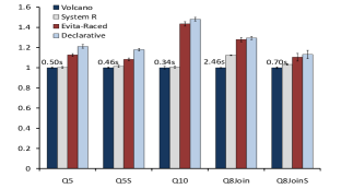
(a) Execution time (normalized to Volcano)

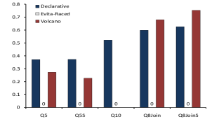
(b) Pruning ratio: plan table entries

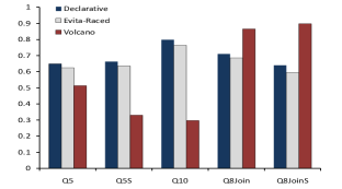
(c) Pruning ratio: plan alternatives

Figure 4: Performance comparison for initial query optimization, across different optimizer architectures

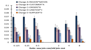
(a) Execution time (normalized to Volcano)

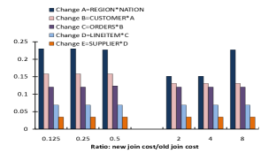
(b) Update ratio: plan table entries

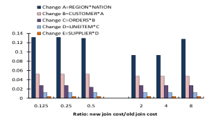
(c) Update ratio: plan alternatives

Figure 5: Performance during incremental re-optimization of TPC-H Q5 — change to join selectivity estimate

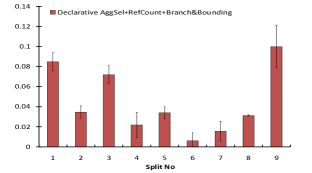
(a) Execution time (normalized to Volcano)

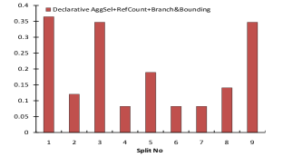
(b) Update ratio: plan table entries

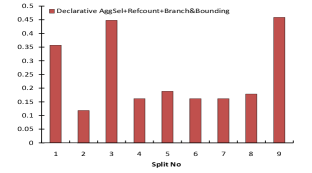
(c) Update ratio: plan alternatives

Figure 6: Performance during incremental re-optimization of TPC-H Q5 — updates to costs based on real execution over skewed data

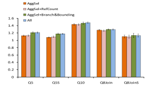
(a) Execution time (normalized to Volcano)

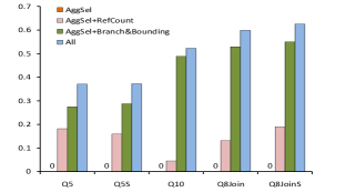
(b) Pruning ratio: plan table entries

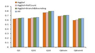
(c) Pruning ratio: plan alternatives

Figure 7: Performance breakdown of pruning techniques for initial optimization, across full query workload

In this section, we discuss the implementation and evaluate the performance of our declarative optimizer: both versus other strategies, and as a primitive for adaptive query processing. (Note that we reuse existing adaptive techniques from tukwila-04 ; cape-04 ; our focus is on showing that incremental re-optimization improves these.)

We implemented the optimizer as 10 datalog rules (see Appendix) plus 8 external functions (involving histograms, cost estimation, and expression decomposition). Our goal was to implement as a proof of concept the common core of optimizer techniques — not an exhaustive set. We executed the optimizer in a modified version of the ASPEN system’s query engine recursive-views , as obtained from its authors. To support the pruning and incremental update propagation features in this paper, we added approximately 10K lines of code to the query engine. In addition, we developed a plan generator to translate the declarative optimizer into a dataflow graph as in Figure 1. Our experiments were performed on a single local node.

For comparison, we implemented in Java a Volcano-style top-down query optimizer and a System-R-style dynamic programming optimizer, which reuse the histogram, cost estimation, and other core components as our declarative optimizer. We also built a variant of our declarative optimizer that only uses the pruning strategies of the Evita Raced declarative optimizer evita-raced . Wherever possible we used common code across the implementations.

Experimental Workload.

For repeated optimization scenarios we use TPC-H queries, with data from the TPC-H and skewed TPC-D data generators tpcd (Scale Factor 1, with Zipfian skew factor 0 for the latter). We focused on the single-block SQL queries: Q1, Q3, Q5, Q6 and Q10. (Q1 and Q6 are aggregation-only queries; Q3 joins 3 relations; Q10 joins 4; and Q5 joins 6 relations). Our experiments showed that Q1, Q3, and Q6 are all simple enough to optimize that (1) there is not a compelling need to adapt, since there are few plan alternatives; (2) they completed in under 80msec on all implementations. (The declarative approach tended to add 10-50msec to these settings, as it has higher initialization costs.) Thus we focus our presentation on join queries with more than 3-way joins. To create greater query diversity, we modified the 4-way and larger join queries by removing aggregation — we constructed a simplified query Q5S. Finally, to test scale-up to larger queries, we manually constructed an eight-way join query, Q8Join, and its simplified version (removing aggregates), Q8JoinS. For adaptive stream processing we used the Linear Road benchmark linearRoad : We modified the largest query, called SegToll. We show our new queries Q8Join and SegTollS in Table 2.

Q8Join: SELECT c_name, p_name, ps_availqty, s_name, o_custkey, r_name, n_name, sum(l_extendedprice * (1 -l_discount)) FROM orders, lineitem, customer, part, partsupp, supplier, nation, region WHERE o_orderkey = l_orderkey and c_custkey = o_custkey and p_partkey = l_partkey and ps_partkey = p_partkey and s_suppkey = ps_suppkey and r_regionkey = n_regionkey and s_nationkey = n_nationkey GROUPBY c_name, p_name, ps_availqty, s_name, o_custkey, r_name, n_name;

SegTollS: SELECT r1_expway, r1_dir, r1_seg, COUNT(distinct r5_xpos) FROM CarLocStr [size 300 time] as r1, CarLocStr [size 1 tuple partition by expway, dir, seg] as r2, CarLocStr [size 1 tuple partition by caid] as r3, CarLocStr [size 30 time] as r4, CarLocStr [size 4 tuple partition by carid] as r5 WHERE r2_expway = r3_expway and r2_dir = 0 and r3_dir = 0 and r2_seg < r3_seg and r2_seg > r3_seg - 10 and r3_carid = r4_carid and r3_carid = r5_carid and r1_expway = r2_expway and r1_dir = r2_dir and r1_seg = r2_seg GROUP BY r5_carid, r2_expway, r2_dir, r2_seg;

Table 2: Queries modified based on TPC-H and LinearRoad benchmark queries used in our experiments

Experimental Methodology.

We aim to answer four questions:

• Can a declarative query optimizer perform at a rate competitive with procedural optimizers, for 4-way-join queries and larger?

• Does incremental query re-optimization show running time and search space benefits versus non-incremental re-optimization, for repeated query execution-over-static-data scenarios?

• How does each of our three pruning strategies (aggregate selection, reference counting, and recursive bounding) contribute to the performance?

• Does incremental re-optimization improve the performance of cost-based adaptive query processing techniques for streaming?

The TPC-H benchmark experiments are conducted on a single local desktop machine: a dual-core Intel Core 2 2.40GHz with 2GB memory running 32-bit Windows XP Professional, and Java JDK 1.6. The Linear Road benchmark experiments are conducted on a single server machine: a dual-core Intel Xeon 2.83GHz with 8 GB memory running 64-bit Windows Server Standard. Performance results are averaged across 10 runs, and 95% confidence intervals are shown. We mark as 0 any results that are exactly zero.

5.1 Declarative Optimization Performance

Our initial experiments focus on the question of whether our declarative query optimizer can be competitive with procedural optimizers based on the System-R (bottom-up enumeration through dynamic programming) and Volcano (top-down enumeration with memoization and branch-and-bound pruning) models. To show the value of the pruning techniques developed in this paper, we also measure the performance when our engine is limited to the pruning techniques developed in Evita Raced evita-raced (where pruning is only done against logically equivalent plans for the same output properties). Recall that all of our implementations share the same procedural logic (e.g., histogram derivation); their differences are in search strategy, dataflow, and pruning techniques.

We begin with a running time comparison among Volcano-style, System-R-style, and declarative implementations (one using our sideways information passing strategies, and one based on the Evita Raced pruning heuristics) — shown in Figure 4 (a). This graph is normalized against the running times for our Volcano-style implementation (which is also included as a bar for visual comparison of the running times). Actual Volcano running times are shown directly above the bar. Observe from the graph that the Volcano strategy is always the fastest, though System-R-style enumeration often approaches its performance due to simpler (thus, slightly faster) exploration logic. Our declarative implementation is not quite as fast as the dedicated procedural optimizers, with an overhead of 10-50%, but this is natural given the extra overhead of using a general-purpose engine and supporting incremental update processing. The Evita Raced-style declarative implementation is marginally faster in this setting, as it does less pruning. We shall see in later experiments that there are significant benefits to our more aggressive strategies during re-optimization — which is our focus in this work.

To better understand the performance of the different options, we next study their effectiveness in pruning the search space. We divide this into two parts: (1) pruning of expression-property entries in the plan table, such that we do not need to compute and maintain any plans for a particular expression yielding a particular property; (2) pruning of plan alternatives for a particular expression-property pair. In terms of the and-or graph formulation of Figure 2, the first case prunes or-nodes and the second prunes and-nodes. We show these two cases in Figure 4 parts (b) and (c). We omit System R from this discussion, as it uses a dynamic programming-based pruning model that is difficult to directly compare.

Part (b) shows that our declarative implementation achieves pruning of approximately 35-80% of the plan table entries, resulting in large reductions in state (and, in many cases, reduced computation). We compare with the strategies used by Evita Raced, which we can see never prunes plan table entries, and with our Volcano-style implementation. Observe that our pruning strategies — which are quite flexible with respect to order of processing — are often more effective than the Volcano strategy, which is limited to top-down enumeration with branch-and-bound pruning. (All pruning strategies’ effectiveness depends on the specific order in which nodes are explored: better pruning is achieved when inexpensive options are considered early. However, in the common case, high levels of pruning are observed.)

Part (c) looks in more detail at the number of alternative query plans that are pruned: here our declarative implementation prunes approximately 55-75% of the space of plans. It exceeds the pruning ratios obtained by the Evita Raced strategies by around 4-8%, and often results in significantly greater pruning than Volcano.

Our conclusions from these experiments are that, even for initial query optimization “from scratch,” a declarative optimizer can be performance-competitive with a procedural one — both in terms of running time and pruning performance. Moreover, given that our plan enumeration and pruning strategies are completely decoupled, we plan to further study whether there are effective heuristics for exploring the search space in our model.

5.2 Incremental Re-optimization

Now that we understand the relative performance of our declarative optimizer in a conventional setting, we move on to study it how it handles incremental changes to costs. A typical setting in a non-streaming context would be to improve performance during the repeated execution of a query, such as for a prepared statement where only a binding changes. The question we ask is how expensive — given a typical update — it is to re-optimize the query and produce the new, predicted-optimal plan.

Note that there exists no comparable techniques for incremental cost-based re-optimization, so we compare the gains versus those of re-running a complete optimization (as is done in tukwila-04 ; cape-04 ). In these experiments, we consider running time — versus the running times for the best-performing initial optimization strategy, namely that of our Volcano-style implementation — as well as how much of the total search space gets re-enumerated. We consider re-optimization under “microbenchmark”-style simulated changes to costs, for synthetic updates as well as observed execution conditions over skewed data. We measured performance across the full suite of queries in our workload. However, due to space constraints, and since the results are representative, we focus our presentation on query Q5.

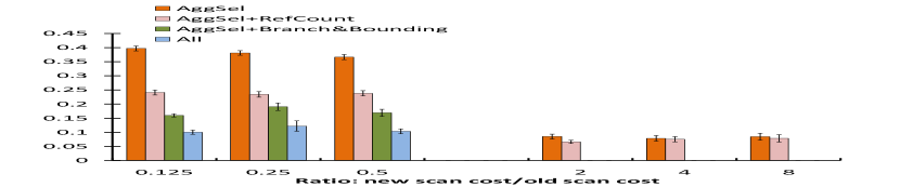
(a) Execution time (vs Volcano)

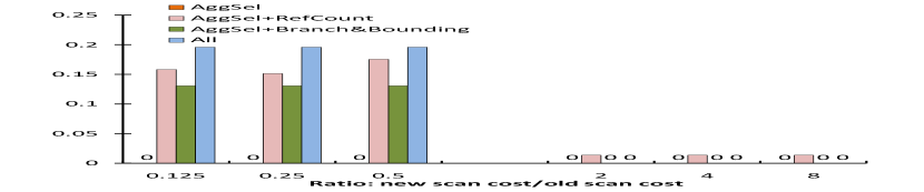
(b) Pruning ratio: plan table entries

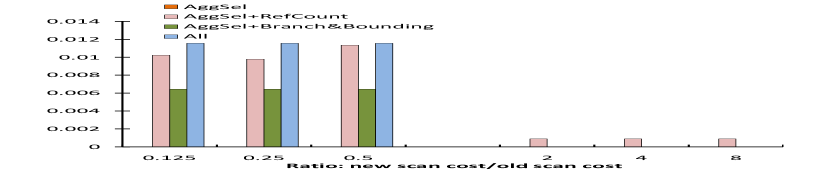
(c) Pruning ratio: plan alternatives

Figure 8: Performance breakdown of pruning techniques during incremental re-optimization of Q5 when $Orders$ has updated scan cost

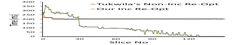
Figure 9: AQP re-opt

5.2.1 Synthetic Changes to Subplan Costs

We first simulate what happens if we discover that an operator’s output is not in accordance with our original selectivity estimates. Figures 5 (a)-(c) show the impact of synthetically injecting changes for each join expression’s selectivity, and therefore the $\mathsf{PlanCost}$ of the related plans and their super-plans. For conciseness in the graph captions, we assign a symbol with each expression, e.g., the first join $Region\Join Nation$ is expression $A$, and the second join expression combines the output of $A$ with data from the $Customer$ table, yielding $B=Customer\Join A$. We expect that changes to smaller subplans will take longer to re-optimize, and changes to larger subplans will take less time (due to the number of recursive propagation steps involved). We separately plot the results of changing each expression’s selectivity value, as we change it along a range from 1/8 the predicted size through 8 times larger than the predicted size. Running times in part (a) are plotted relative to the Volcano implementation’s performance: we see that the speedups are at least a factor of 12, when the lowest-level join cost is updated; going up to over 300, when the topmost join operator’s selectivity is changed. In general the speedups confirm that larger expressions are cheaper to update. We can observe from these last two figures that we recompute only a small portion of the search space.

5.2.2 Changes based on Real Execution

We now look at what happens when costs are updated according to an actual query execution. We took TPC-H Q5 and to gain better generality, we divided its input into 10 partitions (each having uniform distribution and independent variables) that would result in equal-sized output. We optimized the query over one such partition, using histograms from the TPC-H dataset. Then we ran the resulting query over different partitions of skewed data (Zipf skew factor 0.5, from the Microsoft Research skewed TPC-D generator tpcd ); each of which exhibits different properties. At the end we re-optimized the given the cumulatively observed statistics from the partition. We performed re-optimization on each of such interval, given the current plan and the revised statistics.

Figure 6 (a) shows the execution times for each round of incremental re-optimization, normalized against the running time of Volcano. We see that, as with the join re-estimation experiments of Figure 5, there are speedups of a factor of 10 or greater. In terms of throughput, the Volcano model takes 500msec to perform one optimization, meaning it can perform 2 re-optimizations per second; whereas our declarative incremental re-optimizer can achieve 20-60 optimizations per second, and it can respond to changing conditions in 10-100msec. Again, Figure 6 (b) and (c) show that the speedup is due to significant reductions in the amount of state that must be recomputed.

5.3 Contributions of Pruning Strategies

Here we investigate how each of our pruning and incremental strategies from Sections 3 and 4 contribute to the overall performance of our declarative optimizer. We systematically considered all techniques individually and in combination, unless they did not make sense (e.g., reference counting must be combined with one of the other techniques, and branch-and-bound requires aggregate selection to perform pruning of the search space). See Figure 7, where AggSel refers to aggregate selection with source tuple suppression; RefCount refers to reference counting; and Branch&Bounding refers to recursive bounding. We consider aggregate selection in isolation and in combination with the other techniques individually and together. (We also considered the case where none of the pruning techniques are enabled: here running times were over 2 minutes, due to a complete lack of pruning. We omit this from the graphs.)

Figures 7 (a)-(c) compare the three pruning strategies when performing initial optimization on various TPC-H queries. It can be observed that each of the pruning techniques adds a small bit of runtime overhead (never more than 10%) in this setting, as each requires greater computation and data propagation. Parts (b) and (c) show that each technique adds greater pruning capability, however.

Once we move to the incremental setting — shown in Figures 9 (a)-(c) for query Q5 and changes to the $\mathsf{orders}$ table, over different cost estimate changes — we see significant benefits in running time as well as pruned search space. Note that in contrast to our other graphs for incremental re-optimization, plots (b) and (c) isolate the amount of pruning performed, rather than showing the total state updated. We see here that our different techniques work best in combination, and that each increases the amount of pruning.

Our pruning strategies enable incremental updates to be supported with relatively minor space overhead: even for the largest query (Q8Join), the total optimizer state was under 100MB.

5.4 Incremental Reoptimization for AQP

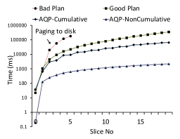
Figure 10: AQP execution time

A major motivation for our work was to facilitate better cost-based adaptive query processing, especially for continuous optimization of stream queries. Our goal is to show the benefits of incremental reoptimization; we leave as future work a broader comparison of adaptive query processing techniques. Our final set of experiments shows how our techniques can be used within a standard cost-based adaptive framework, one based on the data-partitioned model of tukwila-04 where the optimizer periodically pauses plan execution, forming a “split” point from which it may choose a new plan and continue execution. In general, if we change plans at a split point, there is a challenge of determining how to combine state across the split. In contrast to tukwila-04 we chose not to defer the cross-split join execution until the end: rather, we used CAPS’s state migration strategy cape-04 to transfer all existing state from the prior plan into the current one. As necessary, new intermediate state is computed. Note that our data-partitioned model could be combined with other cost-based adaptive schemes such as db2-mqreopt ; DBLP:conf/sigmod/KabraD98 .

To evaluate this setting, we combine unfold the various views comprising the SegToll query from the Linear Road benchmark linearRoad — resulting in a 5-way join plan SegTollS with multiple windowed aggregates. We use the standard Linear Road data generator to synthesize data whose characteristics frequently change.

Per Slice	Re-Opt Time	N.C. Exec Time	Total Time
1s	5.75s	2.20s	7.95s
5s	1.23s	6.82s	8.05s
10s	0.63s	13.35s	13.98s

Table 3: Frequency of Adaptation (20 sec stream)

In the adaptive setting, our goal is to have the optimizer start with zero statistical information on the data, and find a sequence of plans whose running time equals or betters the single best static plan that it would pick given complete information (e.g., histograms).

Figure 10 shows that in fact our incremental AQP scheme provides superior performance to the single best plan (“good single plan”), if we re-optimize every 1 second. This is because the adaptive scheme has a chance to “fit” its plan to the local characteristics of whatever data is currently in the window, rather than having to choose one plan for all data.

A natural question is where the “sweet spot” is between query execution overhead and query optimizer overhead, such that we can achieve best performance. We measured, for a variety of slice sizes, the total running time of query re-optimization and execution over each new slice of data (not considering the additional overhead of state migration, which depends on how similar the plans are). We can see the results in Table 3: there are significant gains in shrinking the interval from 10sec to 5sec, but little more gain to be had in going down to 1sec. Figure 9 helps explain this: as we execute and re-optimize, the overhead of a non-incremental re-optimizer remains constant (about 200 msec each time), whereas the incremental re-optimization time drops off rapidly, going to nearly zero. This means that the system has essentially converged on a plan and that new executions do not affect the final plan.

5.5 Experimental Conclusions

We summarize our evaluation results by providing the answers to the questions raised earlier in this section. First, our declarative query optimizer performs respectably when compared to a procedural query optimizer, for initial optimization: despite the overhead of starting up a full query processor, it gets within 10-50% of the running times of a dedicated optimizer. It more than recovers this overhead during incremental re-optimization, where — across a variety of queries and changes — it typically shows an order-of-magnitude speedup, or better. These gains are largely due to having to re-enumerate a much smaller space of plans than a full re-optimization. In addition, we find that our pruning techniques developed in Section 3 and Section 4 each contribute in a meaningful way to the overall performance of incremental re-optimization. Finally, we show that our incremental re-optimization techniques introduced in this paper help cost-based adaptation techniques provide finer-grained adaptivity and hence better overall performance. Overhead decreases as the system converges on a single plan.

6 Related Work

Our work takes a first step towards supporting continuous adaptivity in a distributed (e.g., cloud) setting where correlations and runtime costs may be unpredictable at each node. Fine-grained adaptivity has previously only been addressed in the query processing literature via heuristics, such as flow rates DBLP:conf/sigmod/AvnurH00 ; viglas-rate , that continuously “explore” alternative plans rather than using long-term cost estimates. Exploration adds overhead even when a good plan has been found; moreover, for joins and other stateful operators, the flow heuristics has been shown to result in state that later incurs significant costs stairs . Other strategies based on filter reordering stanford-aqp are provably optimal, but only work for selection-like predicates. Full-blown cost-based re-optimization can avoid these future costs but was previously only possible on a coarse-grained (high multiple seconds) interval tukwila-04 ; cape-04 .

Our use of declarative techniques to specify the optimizer was inspired in part by the Evita Raced evita-raced system. However, their work aims to construct an entire optimizer using reprogrammable datalog rules, whereas our goal is to effectively perform incremental maintenance of the output query plan. We seek to fully match the pruning techniques of conventional optimizers following the System R systemR and Volcano volcano models. Our results show for the first time that a declarative optimizer can be competitive with a procedural one, even for one-time “static” optimizations, and produce large benefits for future optimizations.

7 Conclusions and Future Work

To build large-scale, pipelined query processors that are reactive to conditions across a cluster, we must develop new adaptive query processing techniques. This paper represents the first step towards that goal: namely, a fully cost-based architecture for incrementally re-optimizing queries. We have made the following contributions:

• A rule-based, declarative approach to query (re)optimization in adaptive query processing systems.

• Novel optimization techniques to prune the optimizer state: aggregate selection, reference counting, and recursive bounding.

• A formulation of query re-optimization as an incremental view maintenance problem, for which we develop novel incremental algorithms to deal with insertions, deletions and updates over runtime cost parameters.

• An implementation over the ASPEN query engine recursive-views , with a comprehensive evaluation of performance against alternative approaches, over a diverse workload, showing order-of-magnitude speedups for incremental re-optimization.

We believe this basic architecture leaves a great deal of room for future exploration. We plan to study how our declarative execution model parallelizes across multi-core hardware and clusters, and how it can be extended to consider the cost of changing a plan given existing query execution state.

A Datalog Rules for Optimizer

R1:	$\mathsf{SearchSpace}$$\mathsf{\mathit{(expr,prop,index,logOp,phyOp,lExpr,}}$
	$\mathsf{\mathit{lProp,rExpr,rProp)}}$ :-
	$\mathsf{Expr}(\mathsf{\mathit{expr,prop}})$, $\mathsf{Fn\_isleaf}(\mathsf{\mathit{expr,{false}}})$,
	$\mathsf{Fn\_split}$$\mathsf{\mathit{(expr,prop,\underline{index},\underline{logOp},\underline{phyOp},\underline{lExpr}}}$,
	$\mathsf{\mathit{\underline{lProp},\underline{rExpr},\underline{rProp})}}$;
R2:	$\mathsf{SearchSpace}$$\mathsf{\mathit{(expr,prop,index,logOp,phyOp,}}$
	$\mathsf{\mathit{lExpr,lProp,rExpr,rProp)}}$ :-
	$\mathsf{SearchSpace}(\mathsf{\mathit{-,-,-,-,-,expr,prop,-,-}})$,
	$\mathsf{Fn\_isleaf}(\mathsf{\mathit{expr,{false}}})$,
	$\mathsf{Fn\_split}$$\mathsf{\mathit{(expr,prop,\underline{index},\underline{logOp},\underline{phyOp},}}$
	$\mathsf{\mathit{\underline{lExpr},\underline{lProp},\underline{rExpr},\underline{rProp})}}$;
R3:	$\mathsf{SearchSpace}$$\mathsf{\mathit{(expr,prop,index,logOp,phyOp,}}$
	$\mathsf{\mathit{lExpr,lProp,rExpr,rProp)}}$ :-
	$\mathsf{SearchSpace}(\mathsf{\mathit{-,-,-,-,-,-,-,expr,prop}})$,
	$\mathsf{Fn\_isleaf}(\mathsf{\mathit{expr,{false})}})$,
	$\mathsf{Fn\_split}$$\mathsf{\mathit{(expr,prop,\underline{index},\underline{logOp},\underline{phyOp},}}$
	$\mathsf{\mathit{\underline{lExpr},\underline{lProp},\underline{rExpr},\underline{rProp})}}$;
R4:	$\mathsf{SearchSpace}(\mathsf{\mathit{expr,prop,-,^{\prime}scan^{\prime},phyOp,-,-,-,-)}})$ :-
	$\mathsf{SearchSpace}(\mathsf{\mathit{-,-,-,-,-,expr,prop,-,-}})$,
	$\mathsf{Fn\_isleaf}(\mathsf{\mathit{expr,{true}}})$, $\mathsf{Fn\_phyOp}(\mathsf{\mathit{prop,\underline{phyOp}}})$;
R5:	$\mathsf{SearchSpace}(\mathsf{\mathit{expr,prop,-,^{\prime}scan^{\prime},phyOp,-,-,-,-}})$ :-
	$\mathsf{SearchSpace}(\mathsf{\mathit{-,-,-,-,-,-,-,expr,prop}})$,
	$\mathsf{Fn\_isleaf}(\mathsf{\mathit{expr,{true}}})$, $\mathsf{Fn\_phyOp}(\mathsf{\mathit{prop,\underline{phyOp}}})$;
R6:	$\mathsf{PlanCost}$$\mathsf{\mathit{(expr,prop,index,logOp,phyOp,-,-,-,-,}}$
	$\mathsf{\mathit{md,cost)}}$ :-
	$\mathsf{SearchSpace}(\mathsf{\mathit{expr,prop,index,logOp,phyOp,-,-,-,-}})$,
	$\mathsf{Fn\_scansummary}(\mathsf{\mathit{expr,prop,\underline{md}}})$,
	$\mathsf{Fn\_scancost}(\mathsf{\mathit{expr,prop,md,\underline{cost}}})$;
R7:	$\mathsf{PlanCost}$$\mathsf{\mathit{(expr,prop,index,logOp,phyOp,}}$
	$\mathsf{\mathit{lExpr,lProp,-,-,md,cost)}}$ :-
	$\mathsf{SearchSpace}$$\mathsf{\mathit{(expr,prop,index,logOp,phyOp,}}$
	$\mathsf{\mathit{lExpr,lProp,-,-}}$, $\mathsf{Fn\_isleaf}(\mathsf{\mathit{lExpr,{false}}})$,
	$\mathsf{PlanCost}(\mathsf{\mathit{lExpr,lProp,-,-,-,-,-,-,-,lMd,lCost}})$,
	$\mathsf{Fn\_nonscansummary}(\mathsf{\mathit{expr,prop,index,logOp,lMd,-,\underline{md}}})$,
	$\mathsf{Fn\_nonscancost}$$\mathsf{\mathit{(expr,prop,index,logOp,phyOp,}}$
	$\mathsf{\mathit{lExpr,lProp,-,-,md,\underline{localCost})}}$,
	$\mathsf{Fn\_sum}(\mathsf{\mathit{lCost,null,localCost,\underline{cost}}})$;
R8:	$\mathsf{PlanCost}$$\mathsf{\mathit{(expr,prop,index,logOp,phyOp,}}$
	$\mathsf{\mathit{lExpr,lProp,rExpr,rProp,md,cost)}}$ :-
	$\mathsf{SearchSpace}$$\mathsf{\mathit{(expr,prop,index,logOp,phyOp,}}$
	$\mathsf{\mathit{lExpr,lProp,rExpr,rProp)}}$,
	$\mathsf{Fn\_isleaf}(\mathsf{\mathit{lExpr,{false}),Fn\_isleaf(rExpr,{false}}})$,
	$\mathsf{PlanCost}(\mathsf{\mathit{lExpr,lProp,-,-,-,-,-,-,-,lMd,lCost}})$,
	$\mathsf{PlanCost}(\mathsf{\mathit{rExpr,rProp,-,-,-,-,-,-,-,rMd,rCost}})$,
	$\mathsf{Fn\_nonscansummary}(\mathsf{\mathit{expr,prop,index,logOp,lMd,rMd,\underline{md}}})$,
	$\mathsf{Fn\_nonscancost}$$\mathsf{\mathit{(expr,prop,index,logOp,phyOp,}}$
	$\mathsf{\mathit{lExpr,lProp,rExpr,rProp,md,\underline{localCost})}}$,
	$\mathsf{Fn\_sum}(\mathsf{\mathit{lCost,rCost,localCost,\underline{cost}}})$;
R9:	$\mathsf{BestCost}(\mathsf{\mathit{expr,prop,min<cost>}})$ :-
	$\mathsf{PlanCost}$$\mathsf{\mathit{(expr,prop,index,logOp,phyOp,}}$
	$\mathsf{\mathit{lExpr,lProp,rExpr,rProp,md,cost)}}$;
R10:	$\mathsf{BestPlan}$$\mathsf{\mathit{(expr,prop,index,logOp,phyOp,}}$
	$\mathsf{\mathit{lExpr,lProp,rExpr,rProp,md,cost)}}$ :-
	$\mathsf{BestCost}(\mathsf{\mathit{expr,prop,cost}})$,
	$\mathsf{PlanCost}$$\mathsf{\mathit{(expr,prop,index,logOp,phyOp,}}$
	$\mathsf{\mathit{lExpr,lProp,rExpr,rProp,md,cost)}}$;

References

- [1] D. J. Abadi, D. Carney, U. Cetintemel, M. Cherniack, C. Convey, S. Lee, M. Stonebraker, N. Tatbul, and S. Zdonik. Aurora: a new model and architecture for data stream management. VLDB J., 12(2), August 2003.
- [2] P. Alvaro, T. Condie, N. Conway, K. Elmeleegy, J. M. Hellerstein, and R. Sears. Boom analytics: exploring data-centric, declarative programming for the cloud. In EuroSys, 2010.
- [3] A. Arasu, M. Cherniack, E. Galvez, D. Maier, A. S. Maskey, E. Ryvkina, M. Stonebraker, and R. Tibbetts. Linear road: a stream data management benchmark. In VLDB, VLDB, pages 480–491. VLDB Endowment, 2004.
- [4] R. Avnur and J. M. Hellerstein. Eddies: Continuously adaptive query processing. In SIGMOD, 2000.
- [5] S. Babu, R. Motwani, K. Munagala, I. Nishizawa, and J. Widom. Adaptive ordering of pipelined stream filters. In SIGMOD, 2004.
- [6] A. Behm, V. R. Borkar, M. J. Carey, R. Grover, C. Li, N. Onose, R. Vernica, A. Deutsch, Y. Papakonstantinou, and V. J. Tsotras. Asterix: towards a scalable, semistructured data platform for evolving-world models. Distributed and Parallel Databases, 29(3), 2011.
- [7] S. Chandrasekaran, O. Cooper, A. Deshpande, M. J. Franklin, J. M. Hellerstein, W. Hong, S. Krishnamurthy, S. Madden, V. Raman, F. Reiss, and M. A. Shah. TelegraphCQ: Continuous dataflow processing for an uncertain world. In CIDR, 2003.
- [8] T. Condie, D. Chu, J. M. Hellerstein, and P. Maniatis. Evita raced: metacompilation for declarative networks. PVLDB, 1(1), 2008.
- [9] A. Deshpande and J. M. Hellerstein. Lifting the burden of history from adaptive query processing. In VLDB, 2004.
- [10] A. Deshpande, Z. Ives, and V. Raman. Adaptive query processing. Foundations and Trends in Databases, 2007.
- [11] G. Graefe. The Cascades framework for query optimization. IEEE Data Eng. Bull., 18(3), 1995.
- [12] G. Graefe and W. J. McKenna. The Volcano optimizer generator: Extensibility and efficient search. In ICDE, 1993.
- [13] A. Gupta, H. Jagadish, and I. S. Mumick. In P. Apers, M. Bouzeghoub, and G. Gardarin, editors, EDBT. Berlin / Heidelberg, 1996.
- [14] A. Gupta, I. S. Mumick, and V. S. Subrahmanian. Maintaining views incrementally. In SIGMOD, 1993.
- [15] Z. G. Ives, A. Y. Halevy, and D. S. Weld. Adapting to source properties in processing data integration queries. In SIGMOD, pages 395–406, 2004.
- [16] N. Kabra and D. J. DeWitt. Efficient mid-query re-optimization of sub-optimal query execution plans. In SIGMOD, 1998.
- [17] L. Liu, C. Pu, R. Barga, and T. Zhou. Differential evaluation of continual queries. Technical Report TR95-17, University of Alberta, June 1995.
- [18] M. Liu, N. E. Taylor, W. Zhou, Z. G. Ives, and B. T. Loo. Recursive computation of regions and connectivity in networks. In ICDE, 2009.
- [19] V. Markl, V. Raman, G. Lohman, H. Pirahesh, D. Simmen, and M. Cilimdzic. Robust query processing through progressive optimization. In SIGMOD, 2004.
- [20] S. Melnik, A. Gubarev, J. J. Long, G. Romer, S. Shivakumar, M. Tolton, and T. Vassilakis. Dremel: Interactive analysis of web-scale datasets. PVLDB, 3(1), 2010.
- [21] R. Motwani, J. Widom, A. Arasu, B. Babcock, S. Babu, M. Datar, G. Manku, C. Olston, J. Rosenstein, and R. Varma. Query processing, resource management, and approximation in a data stream management system. In CIDR, 2003.
- [22] V. Narasayya. TPC-D skewed data generator. 1999.
- [23] P. G. Selinger, M. M. Astrahan, D. D. Chamberlin, R. A. Lorie, and T. G. Price. Access path selection in a relational database management system. In SIGMOD, pages 23–34, 1979.
- [24] S. Sudarshan and R. Ramakrishnan. Aggregation and relevance in deductive databases. In VLDB, 1991.
- [25] S. D. Viglas and J. F. Naughton. Rate-based query optimization for streaming information sources. In SIGMOD, 2002.
- [26] Y. Zhu, E. A. Rundensteiner, and G. T. Heineman. Dynamic plan migration for continuous queries over data streams. In SIGMOD, 2004.