Roaming charges for customers of
cellular-wireless entrant and incumbent providers

1 Introduction

In some countries, cellular wireless roaming charges are prohibitive possibly because the incumbent access-provider is actually or essentially state-run, unlike potential entrants, i.e., the regulator (state) is in a conflict of interest. In other countries, e.g., France, there is a lot of competition among Internet Service (access) Providers (ISPs). Recently, Free purchased a spectrum license to compete in the 4G market. Free is an established discount broadband (wired) ISP likely intending to bundle its existing offerings with cellular wireless. The cellular-wireless incumbents such as Orange disputed Free’s position on roaming charges for its customers while Free builds out its wireless infrastructure and offers highly discounted access rates to attract customers (though Free’s service is quota limited and considered of poorer quality and support, the latter particularly through physical store-fronts) [3]. Orange does lease some of its existing infrastructure to third-party discount providers such as Virgin Wireless (which does not offer bundled services in direct competition with Orange).

The Canadian government also recently considered regulating roaming charges [2] for similar reasons: the entrant wishes relatively low roaming charges so as to be able to offer competitive prices and attract customers while not operating at a severe loss in the short term, whereas the incumbents demand that their higher operating costs are respected including minimally profitable legacy services (e.g., telephony) that they are obliged to maintain. Left to the incumbents, roaming charges may rise to create a barrier to entry into the cellular wireless market.

We consider two competing cellular wireless access providers, indexed 1 and 2, that serve overlapping areas. The coverage lapses of the entrant 2 can be accommodated by the incumbent 1, but not vice versa, i.e., the entrant 2 has much less deployed infrastructure than incumbent 1. So as not to trivialize matters, we assume that the entrant attempts to maintain profitability while it grows its cellular wireless access infrastructure. The roaming charge is assumed regulated, i.e., it’s not controlled by either access provider.

2 Asymmetric case with large incumbent (1) and a small entrant (2)

2.1 Demand response and ISP-player utilities

Let $\phi$ be the fraction of the entrant’s demand that roams and let $r$ be the associated roaming charges per unit demand. We assume that the effective price of the entrant’s customers is $p_{2}+\phi r$, where $p_{k}$ is the access price for the $k$th ISP.

We use a model of demand that considers both response to price and congestion as in e.g., [4], but in our model the congestion based term implicitly depends on demand itself so that the incumbent and entrant demands, respectively, satisfy [5]:

$$D_{1} = D_{\max}(1-\delta\bar{p})\frac{p_{2}+\phi r}{p_{1}+p_{2}+\phi r}g_{1}(D_{1}+\phi D_{2},B_{1})$$ (1)

$$D_{2} = D_{\max}(1-\delta\bar{p})\frac{p_{1}}{p_{1}+p_{2}+\phi r}g_{2}((1-\phi)D_{2},B_{2})$$ (2)

where:

• The first term accounts for how total demand is sensitive to price, here assumed linearly decreasing with average access price from maximum,

  $$\bar{p} = \frac{p_{1}+(p_{2}+\phi r)}{2},$$ (3)

  where $\delta D_{\max}$ is the demand sensitivity to price.

• The second (competition) factor models how demand is divided between the ISPs based on their access price, i.e., ISP $k$’s demand is inversely proportional to $p_{k}$, e.g., [1].

• The third factor models how demand depends on congestion via a “demand capacity” parameter $B$ and “headroom” parameter $\gamma>0$ [5]: $g(D,B)$ decreases with $D<B-\gamma$ and increases with $B$, $g(0,B)\equiv 1\equiv g(D,\infty)$ and $g(B-\gamma,B)\equiv 0$. For example, a nonlinear $g(\cdot,B)$ based on the mean delay of an M/M/1 queue [7] is $g(D,B)=(1-\gamma/(B-D))/(1-\gamma/B)$. A simpler, linearized congestion factor is $g(D,B)=1-D/(B-\gamma)$.

The incumbent and entrant ISP utilities are, respectively,

$$U_{1}(p_{1},p_{2}) = (p_{1}-c_{d,1})D_{1}+(r-c_{d,1})\phi D_{2}-c_{b,1}B_{1}$$

$$U_{2}(p_{2},p_{1}) = (p_{2}-(1-\phi)c_{d,2})D_{2}-c_{b,2}B_{2}$$

where $c_{b}$ is demand-independent operational expenditures (op-ex), including amortized capital expenditures, cap-ex) per-unit infrastructure resource ($B$), and $c_{d}$ is per-unit demand-dependent op-ex.

2.2 Game set-up, simplifications and discussion of objectives

We now assume that demand-dependent op-ex $c_{d}$ are negligible for analytical simplicity. The infrastructure based costs will not impact Nash equilibrium prices and will complicate our notion of “fairness” regarding roaming charges, cf., (7). So in this section, we will assume $c_{b}\approx 0$ too. We also consider the system free of congestion, i.e., $g_{1},g_{2}\approx 1$ in (1) and (2). Thus, we will consider the following utility functions

$$U_{1}(p_{1},p_{2})/D_{\max} = p_{1}(1-\delta\bar{p})\frac{p_{2}+\phi r}{p_{1}+p_{2}+\phi r}+r\phi(1-\delta\bar{p})\frac{p_{1}}{p_{1}+p_{2}+\phi r}$$ (4)

$$U_{2}(p_{2},p_{1})/D_{\max} = p_{2}(1-\delta\bar{p})\frac{p_{1}}{p_{1}+p_{2}+\phi r}$$ (5)

Assuming both sets of customers roam in the same domain (that of the incumbent), we can take the roaming factor

$$\phi = \frac{B_{1}-B_{2}}{B_{1}}~{}=~{}1-\frac{B_{2}}{B_{1}}.$$ (6)

Thus, the simplified system has three positive parameters in addition to initial prices (play-actions): $\phi,\delta,r$. Again, we assume that the roaming factor $r$ is set by a regulator.

2.3 Objectives

Assuming $B_{1}\gg B_{2}$ ($\phi\approx 1$), our objective herein is to determine the Nash equilibrium (NE) prices $p^{*}_{1},p^{*}_{2}$ and see how the NE utilities $U^{*}$ depend on the roaming charge, $r$. The impact of the demand-sensitivity-to-price parameter $\delta D_{\max}$ will be to simply shift and scale the NE prices.

Specifically, we want to see whether fairness is achieved at NE, i.e., whether net revenue is proportional to expenditures:

$$\frac{U_{1}^{*}(r)}{B_{1}} = \frac{U_{2}^{*}(r)}{B_{2}},$$ (7)

equivalently under (6), whether

$$(1-\phi)U_{1}^{*}(r)-U_{2}^{*}(r) = 0.$$ (8)

2.4 Analytical results for simplified system

An “interior” (strictly positive, finite) solution to the first-order necessary conditions (FONC),

$$\frac{\partial U_{1}}{\partial p_{1}} =~{}0~{}= \frac{\partial U_{2}}{\partial p_{2}},$$ (9)

of (4) and (5) is a symmetric one where both NE prices

$$p_{1}^{*},p_{2}^{*} = \frac{1}{4\delta}\left(-2\delta r\phi+1+\sqrt{4\delta r\phi+1}\right)~{}>~{}0$$ (10)

when

$$\delta r\phi < 2,$$ (11)

i.e., when there are feasible prices $(p_{1},p_{2})$ according to

$$p_{1}+p_{2} \leq -r\phi+2/\delta.$$

Indeed, it can be directly verified that $p_{1}^{*}+p_{2}^{*}=2p_{1}^{*}=2p_{2}^{*}<-r\phi+2/\delta$.

These prices also satisfy $\partial^{2}U_{1}/\partial p_{1}^{2},~{}\partial^{2}U_{2}/\partial p_{2}^{2}<0$, with strictly positive utilities $U_{1}^{*},U_{2}^{*}>0$ under (11), so that indeed they are “locally Nash.” The other solutions of the FONC (9) either have $p_{2}^{*}<0$ (i.e., extraneous) or $p_{1}^{*}=0$. But if $p_{1}^{*}=0$ then $U_{1}^{*}=0=U_{2}^{*}$. Also, if $p_{2}=0$ then $\partial U_{2}/\partial p_{2}>0$. So, there are no boundary Nash equilibria and thus (10) is the unique Nash equilibrium.

It can also be directly shown for this model that there is a solution

$$r^{*} := \frac{2(2-\phi)}{\delta(4-3\phi)^{2}}$$ (12)

at which (8) holds. Note that $r^{*}<2(\delta\phi)^{-1}$ for $0\leq\phi<1$. Roaming prices $r<r^{*}$ favor the entrant, otherwise the incumbent, cf., next subsection.

2.5 Numerical results

We considered the example with $\delta=1$ and $\phi=0.9=1-B_{2}/B_{1}$. For the model without congestion under (11), the two “best response” curves for $r=0.8$ are given in Figure 1. That is, the first curve has vertical distance to the $x$-axis,

$$p_{2}^{*}(p_{1}) = \mbox{arg}\max_{0\leq p_{2}\leq p_{\max}}U_{2}(p_{2},p_{1}).$$

The second curve has horizontal distance to the $y$-axis,

$$p_{1}^{*}(p_{2}) = \mbox{arg}\max_{0\leq p_{1}\leq p_{\max}}U_{1}(p_{1},p_{2}).$$

These curves meet at the Nash equilibrium, here $(p_{1}^{*},p_{2}^{*})\approx(0.38,0.38)$ which is consistent with (10).

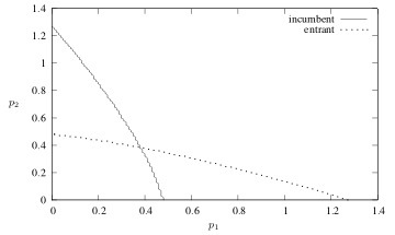
Figure 1: Best-response curves for $\phi=0.9,\delta=1,r=0.8$

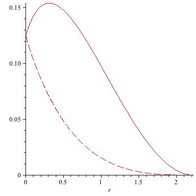
Figure 2: Utilities of the incumbent $U_{1}^{*}(r))/D_{\max}$ (solid line) and entrant $U_{2}^{*}(r)/D_{\max}$ (dashed line) versus roaming charge $r$ with $\phi=0.9,\delta=1$

We also numerically verified that Nash-equilibrium utilities $U_{1}^{*}(r)$ and $U_{2}^{*}(r)$ are positive, see Figure 2. Both decrease and reach zero at $r=2(\delta\phi)^{-1}=20/9$ (again, a point where the only feasible prices are $p_{1}=0=p_{2}$). Note that utilities are generally higher for lower roaming charges in our simple model.

In Figure 3, we plot the “fairness” expression in (8) and verify that (8) holds at $r^{*}\approx 1.3<20/9$, consistent with (12). And we see from this figure how roaming prices $r<r^{*}$ favor the entrant, otherwise the incumbent.

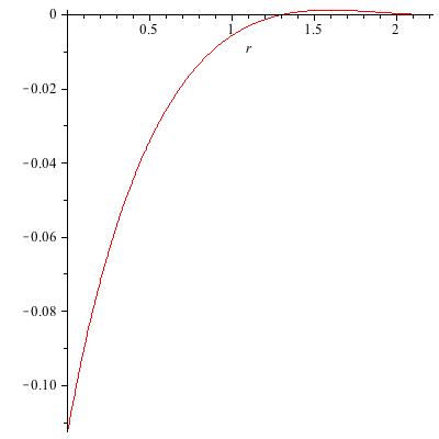
Figure 3: $((1-\phi)U_{1}^{*}(r)-U_{2}^{*}(r))/D_{\max}$ versus roaming charge $r$ with $\phi=0.9,\delta=1$

3 Future work

Recall that we assumed negligible op-ex, i.e., assumed $c_{b},c_{d}\approx 0$. Depending on the situation, op-ex per unit demand might be lower for the entrant (e.g., only present in areas involving cheaper deployment costs and higher customer density) or for the incumbent (generally owing to greater scale of operations). Such a discrepancy could be accounted for in our “fairness” condition (7). Future work will also consider the effects of congestion, more complex price-competition and price-sensitivity models, and multiple competing incumbents and entrants (as in [1]).

Acknowledgment:

We wish to thank Dr. Ashraf Al Daoud for a preliminary discussion on regulating roaming charges.

References

- [1] S. Caron, G. Kesidis and E. Altman. “Application Neutrality and a Paradox of Side Payments”, in Proc. ACM ReArch, Philadelphia, Nov. 30, 2010. See also http://arxiv.org/abs/1006.3894
- [2] CBC News. Domestic wireless roaming fees to be capped Fines coming for violations of Wireless Code. Dec. 18, 2013, Available at http://www.cbc.ca/news/technology/domestic-wireless-roaming-fees-to-be-capped-1.2468642
- [3] S. Shankland. Price war cuts roaming fees for French mobile customers. Jan. 30, 2014, Available at http://www.cnet.com/news/price-war-cuts-roaming-fees-for-french-mobile-customers/
- [4] R. Johari, G.Y. Weintraub, and B. Van Roy Investment and Market Structure in Industries with Congestion. Operations Research 58(5):1303–1317, Sept.–Oct. 2010.
- [5] G. Kesidis. Variation of “The effect of caching on a model of content and access provider revenues in information-centric networks”. Technical report at http://arxiv.org/abs/1304.1942
- [6] G. Kesidis. A simple two-sided market model with side-payments and ISP service classes. In Proc. IEEE INFOCOM Workshop on Smart Data Pricing, Toronto, May 2014.
- [7] R.W. Wolff. Stochastic Modeling and the Theory of Queues. Prentice-Hall, Englewood Cliffs, NJ, 1989.