Mobile impurities and orthogonality catastrophe in two-dimensional vortex lattices

Abstract

We investigate the properties of a neutral impurity atom coupled with the Tkachenko modes of a two-dimensional vortex lattice in a Bose-Einstein condensate. In contrast with polarons in homogeneous condensates, the marginal impurity-boson interaction in the vortex lattice leads to infrared singularities in perturbation theory and to the breakdown of the quasiparticle picture in the low energy limit. These infrared singularities are interpreted in terms of a renormalization of the coupling constant, quasiparticle weight and effective impurity mass. The divergence of the effective mass in the low energy limit gives rise to a power law singularity in the impurity spectral function and provides an example of an emergent orthogonality catastrophe in a bosonic system.

I Introduction

Ultracold quantum gases are by now well established as an alternative platform for realizing interacting models originally developed in condensed matter physics bloch . Moreover, the high controllability of model parameters and system dimensionality allows one to explore exotic phases of matter that could never be reached in conventional experiments involving electrons in metals. In particular, recent techniques for cooling two-component mixtures have opened the way to investigating polaron physics via the interaction of a low density of “impurity” atoms with the environment formed by another majority species mathey ; StrongCoup ; jaksch ; pupillo ; zwierlein ; drevessen3 ; kohl ; zaccanti1 ; berciu ; fukuhara ; balewski ; zaccanti2 . The properties of these atomic polarons can be probed using species-selective radio-frequency spectroscopy T1 ; shashi , and the experimental results can be compared quantitatively with predictions from microscopic many-body theory even in the strong coupling limit zaccanti2 .

In ultracold atom systems, there is a diverse set of collective modes with which the impurity can be dressed to form a polaron. For instance, the interaction of impurities with particle-hole pairs of a Fermi sea has been studied in Fermi gases with a large population imbalance kohl ; zwierlein ; zaccanti1 ; nascimbene ; parish ; schmidt . By tuning the atomic $s$-wave interaction, one can even switch between the regimes of attractive and repulsive polarons. In the case of a background formed by bosonic atoms, polarons are formed when the impurities are dressed by the Bogoliubov phonons of a condensate jaksch ; drevessen3 . Interestingly, the phonon-mediated interaction between impurities can lead to the formation of polaron clusters and “localization” in the sense of broadening of the momentum distribution jaksch .

In Ref. PRL111 we proposed a novel addition to the polaron family which we referred to as the “Tkachenko polaron”. The latter originates when an impurity atom is immersed in a two-dimensional (2D) vortex lattice Science ; cornell formed by ultracold bosons in the mean field quantum Hall regime PRL87 ; muller . The vortex lattice is distinguished by the existence of so-called Tkachenko modes with parabolic dispersion sonin ; baym ; sinova ; shlyapnikov ; shlyapnikov2 , as opposed to the usual linear dispersing phonons of a 2D crystal. Using perturbation theory, we showed that at weak coupling the polaron spectral function has a Lorentzian lineshape with a decay rate linearly proportional to the polaron energy. On the other hand, a renormalization group (RG) analysis of the effective field theory in the continuum limit reveals that the interaction between the impurity and the bosonic modes with quadratic dispersion in 2D is marginally relevant. This implies that the effective coupling grows as the energy decreases, leading to an anomalous broadening of the spectral function and the breakdown of the quasiparticle picture in the long wavelength limit.

In this work we wish to clarify the properties of the low energy limit of Tkachenko polarons. We shall show that the effective Hamiltonian flows under the RG to a line of fixed points in which the impurity mass diverges while the impurity-boson coupling is enhanced but remains finite. In this limit the heavy impurity is dressed by a diverging number of low-energy modes, a characteristic feature of the orthogonality catastrophe (OC) phenomenon mahan ; noziere ; noziere2 ; noziere3 . The signature of this phenomenon on the impurity spectral function is the development of an approximate power-law singularity at low energies. There are two unique aspects about the OC in our model. First, it arises in an impurity model with a background of bosonic excitations, whereas the usual OC (which has also been studied in the context of cold atoms T2 ; PRX ; demler ; Ap2 ) occurs in fermionic systems. Second, while the usual OC requires a localized impurity, in our case we can start with a mobile impurity (i.e. with a finite mass), and the localization emerges asymptotically as the effective impurity mass diverges in the low energy limit. We can then speak of self-trapping in the sense that the time scales over which the impurity moves through the lattice become anomalously large. Both of these aspects stem from the peculiar dispersion of Tkachenko modes, which exhibit a finite density of states in the low energy limit, leading to infrared singularities in perturbation theory. We note that similar infrared singularities occur in one-dimensional systems kantian .

The paper is organized as follows. In Section II we review results for the Tkachenko polaron model in the weak coupling regime PRL111 . The RG flow of the parameters in the effective model is calculated in Section III. Next, in Section IV, we analyze the low energy fixed points by applying a canonical transformation to extract the power law singularity characteristic of the OC. This section presents our main results concerning the spectral function for the mobile impurity in the low energy limit. In Section V we point out connections to existing experiments and the viability of detecting our predictions. Finally, we summarize our results in Section VI.

II Weak coupling regime of the light Tkachenko polaron

II.1 Continuum model

We consider a two-component boson mixture with a large population imbalance between species $A$ (majority atoms) and $B$ (impurity atoms). We assume that both species occupy the ground state of a strongly confining potential in the $z$ direction, so the system is effectively 2D. Within the $xy$ plane the bosons are confined by a weaker harmonic trap $V_{ext}(\bf{r})$.

We would like to induce a vortex lattice in the majority species while keeping the impurities with nearly free dispersion. This is not possible in a rotating trap since the Hamiltonian in the rotating frame contains an effective magnetic field that couples to both species cooper , leading to the undesirable effect of Landau quantization of the impurity energy levels. For this reason, we consider instead an artificial vector potential ${\bf A}(\bf{r})$ dalibard2 ; lin that corresponds to an effective uniform magnetic field in the laboratory frame and couples selectively to $A$ atoms. The essential idea to implement species-specific artificial gauge fields for neutral atoms is to produce Berry phases by combining the internal atomic structure with carefully engineered optical potentials, for instance via spatial gradients of detuning or Rabi frequency spielman . The interacting Hamiltonian in the presence of the gauge fields is $H=H_{A}+H_{B}+H_{int}$, with

$$H_{A} = \int d^{2}r\Bigg{[}\hat{\psi}_{A}^{\dagger}\frac{(-i\hbar\nabla-{\bf A})^{2}}{2m_{A}}\hat{\psi}_{A}^{\phantom{\dagger}}+V_{ext}(\mathbf{r})\,\hat{\psi}_{A}^{\dagger}\hat{\psi}_{A}$$

$$+ \frac{g_{A}}{2}(\hat{\psi}_{A}^{\dagger}\hat{\psi}_{A}^{\phantom{\dagger}})^{2}\Bigg{]},$$

$$H_{B} = \int d^{2}r\left[\hat{\psi}_{B}^{\dagger}\frac{(-i\hbar\nabla)^{2}}{2m_{B}}\hat{\psi}_{B}^{\phantom{\dagger}}+V_{ext}(\mathbf{r})\,\hat{\psi}_{B}^{\dagger}\hat{\psi}_{B}\right.$$

$$\left.+\frac{g_{B}}{2}(\hat{\psi}_{B}^{\dagger}\hat{\psi}_{B}^{\phantom{\dagger}})^{2}\right],$$

$$H_{int} = g_{AB}\int d^{2}r\,\hat{\psi}_{A}^{\dagger}\hat{\psi}_{A}^{\phantom{\dagger}}\hat{\psi}_{B}^{\dagger}\hat{\psi}_{B}^{\phantom{\dagger}}.$$ (1)

Here each species is described by a creation (annihilation) operator $\hat{\psi}_{i}(\mathbf{r})\;[\hat{\psi}_{i}^{{\dagger}}(\mathbf{r})]$, with $i=A,B$. The intra-species repulsive contact interactions for the 2D system are given by $g_{i}=2\sqrt{2\pi}\hbar^{2}a_{i}/m_{i}l_{0}$, and the inter-species interaction is $g_{AB}=\sqrt{2\pi}\,\hbar^{2}\,a_{AB}/\mu l_{0}$, where $\mu=m_{i}m_{i}/(m_{i}+m_{j})$ is the reduced mass, $a_{A},a_{B},a_{AB}$ are the corresponding three-dimensional $s$-wave scattering lengths, and $l_{0}=\sqrt{\hbar/m_{A}\omega_{0}}$ is the axial oscillator length for a harmonic trapping potential with frequency $\omega_{0}$ in the $z$ direction.

The vorticity of the $A$ subsystem is characterized by the magnetic length $l=\sqrt{\hbar/\mathcal{B}}$, with $\mathcal{B}=|\nabla\times\mathbf{A}|=$ const., or by the cyclotron frequency $\Omega=\mathcal{B}/m_{A}$. At critical vorticity, i.e. when the oscillator length of $V_{ext}$ matches the magnetic length, the residual confining potential for $A$ atoms in the $xy$ plane vanishes and the system is effectively in an infinite plane geometry shlyapnikov2 . Let $n_{A}=N_{A}/\mathcal{S}$ denote the average 2D density for $N_{A}$ atoms distributed over an area $\mathcal{S}$. The 2D density of vortices is $n_{V}=N_{V}/\mathcal{S}=(\pi l^{2})^{-1}$, and the filling factor is $\nu=N_{A}/N_{V}=n_{A}\pi l^{2}$ . In the mean-field quantum Hall regime PRL87 ; muller $g_{A}n_{A}\ll\hbar\Omega$, a good starting point is to consider that all $A$ atoms occupy the same macroscopic quantum state given by a linear superposition of lowest Landau level states. The mean field state that minimizes the energy is the Abrikosov vortex lattice state $\psi_{A}(\mathbf{r})=\sqrt{n_{A}}\varphi_{A}(\mathbf{r})$, where $\varphi_{A}(\mathbf{r})=(2\varsigma)^{1/4}\;\vartheta_{1}(\sqrt{\pi\varsigma}z,\rho)\;e^{z^{2}/2}\;e^{-|z|^{2}/2}$ is a normalized wavefunction involving the Jacobi theta function $\vartheta_{1}$ with parameters $z=(x+iy)/l$, $u=-1/2$, $\varsigma=\sqrt{3}/2$, $\tau=u+i\varsigma$, and $\rho=\exp(i\pi\tau)$. One can check that the density profile $|\varphi_{A}(\mathbf{r})|^{2}$ corresponds to a triangular vortex array shlyapnikov2 .

Before advancing with the model, a few remarks about the stability of the vortex lattice are in order. In the mean field regime, the number of vortices $N_{V}$ is well below the number of $A$ atoms. In other words, the filling factor is large, $\nu\gg 1$; experimental values of $\nu\sim 500$ have been reported cornell ; cooper . It is known that even at $T=0$ the vortex lattice state lacks long-range phase coherence sinova . However, the crystalline density profile is stable against quantum melting for filling factors above a critical value $\nu_{c}\sim 6$ cooper2 . Below this critical value, incompressible quantum Hall phases of bosons have been predicted cooper . Here we are interested in the regime $N_{B}\ll N_{V}\ll N_{A}$, where we can safely assume that the vortex lattice is stable against its own quantum fluctuations as well as against perturbations induced by coupling to dilute $B$ atoms.

The excitation spectrum of the vortex lattice can be obtained by expanding $H_{A}$ about the mean field solution sinova ; baym ; shlyapnikov . The spectrum contains one gapped “inertial” mode and one gapless mode — the Tkachenko mode — with parabolic dispersion in the low energy limit. The latter corresponds to the Goldstone boson expected from spontaneous breaking of translational and rotational symmetries in the vortex lattice state. The parabolic dispersion may seem unusual, but is consistent with the counting of Goldstone modes for non-relativistic systems nielsen ; watanabe . In the mean field regime the inertial mode gap (of order $\hbar\Omega$) is large and the lattice dynamics is dominated by the gapless Tkachenko mode. Following shlyapnikov , we expand the field operator for $A$ atoms about the mean field state in the form $\hat{\psi}_{A}=\psi_{A}+\delta\hat{\psi}_{A}$, with

$$\delta\hat{\psi}_{A}(\mathbf{r})=\frac{1}{\sqrt{\mathcal{S}}}\sum_{\mathbf{q}\in\textrm{BZ}}\left[u_{\mathbf{q}}(\mathbf{r})a_{\mathbf{q}}^{\phantom{\dagger}}-v_{\mathbf{q}}(\mathbf{r})a_{\mathbf{q}}^{\dagger}\right].$$ (2)

Here $a_{\mathbf{q}}$ is the annihilation operator for the Tkachenko mode with wave vector $\mathbf{q}$ defined in the Brillouin zone of the triangular lattice and $u_{\mathbf{q}}(\mathbf{r})$, $v_{\mathbf{q}}(\mathbf{r})$ are solutions of the projected Bogoliubov-de Gennes equations. For $q\ll l^{-1}$, the dispersion relation is $\hbar\omega_{\mathbf{q}}\approx\hbar^{2}q^{2}/2M$, with the effective mass $M\sim(\hbar\Omega/n_{A}g_{A})m_{A}\gg m_{A}$.

The Tkachenko polaron is defined as the problem of a single $B$ atom propagating in the background of a vortex lattice state PRL111 . The first difference from a homogeneous condensate appears to zeroth order in the fluctuations $\delta\hat{\psi}_{A}$, in the form of a static lattice potential obtained by substituting the mean field solution for $\psi_{A}$ in $H_{int}$ in Eq. (II.1). However, in the limit of weak interspecies interaction $n_{A}g_{AB}\ll\hbar\Omega$ and small momenta $q\ll l^{-1}$, the effective impurity mass $m_{B}$ is only weakly renormalized by the shallow lattice potential. We assume $m_{B}\sim m_{A}\ll M$, so that the impurity is light compared to the Tkachenko boson. Hereafter we set $m_{B}=m$ to lighten the notation.

The term generated by $H_{int}$ to first order in the fluctuation $\delta\hat{\psi}_{A}$ is an effective “impurity-phonon” interaction, with phonons replaced by Tkachenko modes. In the continuum, large-polaron limit $k,q\ll l^{-1}$, we obtain PRL111

$$H_{imp-ph}\approx\frac{\lambda}{\sqrt{\mathcal{S}}}\sum_{\textbf{k},\textbf{q}}|\mathbf{q}|\hat{b}_{\textbf{k+q}}^{\dagger}\,\hat{b}^{\phantom{\dagger}}_{\textbf{k}}\,(\hat{a}_{\textbf{q}}+\hat{a}_{-\textbf{q}}^{\dagger}),$$ (3)

where $\hat{b}_{\mathbf{k}}$ is the annihilation operator for impurities in states with momentum $\mathbf{k}$ and $\lambda\sim\sqrt{\nu}g_{AB}$ is the impurity-boson coupling constant. Note that $\lambda$ is enhanced by the large filling factor $\nu\gg 1$. We finally obtain the 2D Tkachenko polaron model PRL111

$$H = H_{ph}+H_{imp}+H_{imp-ph}$$ (4)

$$= \sum_{\mathbf{q}}\omega_{\mathbf{q}}\,\hat{a}_{\mathbf{q}}^{\dagger}\,\hat{a}^{\phantom{\dagger}}_{\mathbf{q}}+\sum_{\mathbf{k}}\,\varepsilon_{\mathbf{k}}\hat{b}_{\mathbf{k}}^{\dagger}\,\hat{b}^{\phantom{\dagger}}_{\textbf{k}}$$

$$+\frac{\lambda}{\sqrt{\mathcal{S}}}\sum_{\mathbf{k},\mathbf{q}}|\mathbf{q}|\hat{b}_{\mathbf{k}+\mathbf{q}}^{\dagger}\hat{b}^{\phantom{\dagger}}_{\mathbf{k}}\,(\hat{a}_{\mathbf{q}}+\hat{a}_{-\mathbf{q}}^{\dagger}),$$

where $\omega_{\mathbf{q}}=\hbar^{2}q^{2}/2M$ and $\varepsilon_{\mathbf{k}}=\hbar^{2}k^{2}/2m$ are the parabolic dispersion relations of Tkachenko modes and impurity atoms, respectively. In the following we set $\hbar=1$.

II.2 Perturbative result for polaron Green’s function

In order to calculate the polaron properties, it is natural to use diagrammatic many-body theory. The Green’s function of the impurity can be written as

$$G(\mathbf{k},\omega)=[\omega-\varepsilon_{\mathbf{k}}-\Sigma(\mathbf{k},\omega)]^{-1},$$ (5)

where $\varepsilon_{\mathbf{k}}=k^{2}/2m$ is the bare impurity dispersion and $\Sigma(\mathbf{k},\omega)$ is the self-energy. The polaron energy $E_{\mathbf{k}}$ is found as the solution to the implicit equation $E_{\mathbf{k}}\simeq\varepsilon_{\textbf{k}}+\textrm{Re}\Sigma(\mathbf{k},E_{\mathbf{k}})$. For weak interactions, one usually expects that low energy (small $k$ and $\omega$) excitations be quasiparticles that resemble the free particles but with a renormalized mass and a finite lifetime. In this case, the retarded Green’s function for frequencies close to the polaron energy can be cast in the form mahan

$$G_{ret}(\mathbf{k},\omega)\approx\frac{Z}{\omega-E_{\mathbf{k}}+i\gamma_{\mathbf{k}}}.$$ (6)

Here $Z$ is the quasiparticle residue (or field renormalization) given by

$$Z=\left[1-\left.\left(\frac{\partial{\textrm{Re}\Sigma}}{\partial\omega}\right)\right|_{0}\right]^{-1}.$$ (7)

The decay rate is given by

$$\gamma_{\mathbf{k}}=-Z\,\textrm{Im}\Sigma_{ret}(\mathbf{k},E_{\mathbf{k}}).$$ (8)

Eq. (6) implies that the single-particle spectral function,

$$A(\mathbf{k},\omega)=-\frac{1}{\pi}\textrm{Im}G_{ret}(\mathbf{k},\omega),$$ (9)

can be approximated by a Lorentzian peak with weight $Z$ and width $\gamma_{\mathbf{k}}$.

The expansion of the real part of the self-energy to order $k^{2}$ yields a renormalization of the effective mass in the form $E_{\mathbf{k}}\approx k^{2}/2m^{*}$ with

$$\frac{m}{m^{*}}=Z\left[1+m\left.\left(\frac{\partial^{2}\textrm{Re}\Sigma}{\partial k^{2}}\right)\right|_{0}\right].$$ (10)

We have omitted a constant energy shift $E_{0}=\Sigma(\mathbf{k}=0,\omega=0)$, which we absorb in the definition of the polaron ground state energy.

Figure 1: Impurity self-energy (a) and vertex correction Feynman diagram (b). The solid and wavy lines represent free impurity and Tkachenko mode (analogous to a phonon) propagators, respectively.

Let us then consider the weak coupling limit of Hamiltonian (4) and calculate $\Sigma(\mathbf{k},\omega)$ by perturbation theory in $\lambda$. The lowest-order Feynman diagram that contributes to the self-energy contains one Tkachenko mode and impurity propagator in the intermediate state, as shown in Fig. 1a. This diagram yields the retarded self-energy to second order in $\lambda$:

$$\Sigma^{(2)}_{ret}(\mathbf{k},\omega)=\int\frac{d^{2}q}{(2\pi)^{2}}\,\frac{\lambda^{2}|\mathbf{q}|^{2}}{\omega-\omega_{\mathbf{q}}-\varepsilon_{\mathbf{k}+\mathbf{q}}+i\delta},$$ (11)

where $\delta\to 0^{+}$. As shown in Ref. PRL111 , the decay rate to order $\lambda^{2}$ reads

$$\gamma_{\mathbf{k}}\approx-\textrm{Im}\Sigma(k,\varepsilon_{\mathbf{k}})\approx\frac{\lambda^{2}mM^{3}k^{2}}{2(m+M)^{3}}.$$ (12)

The perturbative decay rate is linear in energy, $\gamma_{\mathbf{k}}\propto\varepsilon_{\mathbf{k}}\propto k^{2}$. Therefore, the quasiparticle peak is only marginally defined, since the relative width $\gamma_{\mathbf{k}}/\varepsilon_{\mathbf{k}}$ does not go to zero as $k\to 0$ (cf. the standard example of $\mathbf{k}$ approaching the Fermi surface for quasiparticles in Fermi liquids mahan ). Nonetheless, the relative width can still be small as long as $\lambda m\ll 1$ (assuming $M\gg m$).

The effects of the interaction to order $\lambda^{2}$ are even more pronounced in the real part of the self-energy. Both the quasiparticle residue and the renormalized mass pick up a logarithmic dependence on momentum:

$$Z(k)\approx\left[1+\frac{2\lambda^{2}\mu^{2}}{\pi}\;\ln\left(\frac{\Lambda_{0}}{k}\right)\right]^{-1},$$ (13)

$$m^{*}(k)\approx m+\frac{4\lambda^{2}\mu^{3}}{\pi}\ln\left(\frac{\Lambda_{0}}{k}\right),$$ (14)

where $\Lambda_{0}$ is an ultraviolet momentum cutoff (of the order of $1/l$) and $\mu=mM/(m+M)$ is the reduced mass of the two-body problem in the intermediate state (note $\mu\approx m$ for $m\ll M$). Remarkably, $Z(k)$ decreases and $m^{*}(k)$ increases logarithmically as $k$ decreases. Therefore, the perturbative corrections are infrared singular: Even for $\lambda\mu\ll 1$, the quasiparticle picture breaks down at exponentially small momenta $k\lesssim\Lambda_{0}e^{-\pi/(2\lambda^{2}\mu^{2})}$.

Within the perturbative regime $k\gg\Lambda_{0}e^{-\pi/(2\lambda^{2}\mu^{2})}$, we may include the logarithmic corrections in $\gamma_{\mathbf{k}}$ and $E_{\mathbf{k}}$ in the spirit of RG improved perturbation theory. We find that the relative width of the quasiparticle peak increases logarithmically as $k$ decreases PRL111

$$\frac{\gamma_{\mathbf{k}}}{E_{\mathbf{k}}}\approx\frac{\lambda^{2}m^{2}}{(1+\varrho)^{3}}\left[1+\frac{\lambda^{2}m^{2}(5+\varrho^{2})}{\pi(1+\varrho)^{4}}\ln\frac{\Lambda_{0}}{\varepsilon_{\mathbf{k}}}\right],$$ (15)

where $\varrho=m/M$ is the bare mass ratio.

III Renormalization group analysis

The logarithmic corrections appearing in perturbation theory in Eqs. (13) and (14) can be interpreted in terms of the renormalization of the effective coupling constant $\lambda$ at the scale set by the impurity momentum $k$. Indeed, in Ref. PRL111 we derived perturbative RG equations for $\lambda$ and found it to be marginally relevant in the weak coupling limit. Here we shall generalize the RG flow equations to include the renormalization of the quasiparticle weight and then discuss the low-energy fixed point that arises when $Z(k)\to 0$.

The perturbative RG equations shankar can be derived from the one-loop diagrams in Fig. 1. The self-energy diagram in Fig. 1a and the vertex correction in Fig. 1b are second order and third order in $\lambda$, respectively. We include the quasiparticle residue $Z(k)$ in the Green’s function for the internal impurity lines and consider that the internal momenta are limited by an ultraviolet cutoff $\Lambda$. This cutoff is set by the momentum scale at which we measure correlations of the interacting model, in this case of the order of the impurity momentum, $\Lambda\sim k\ll\Lambda_{0}$. In the RG step, we consider an infinitesimal reduction of the cutoff to a new value $\Lambda^{\prime}=\Lambda\,e^{-d\ell}$, with $d\ell\ll 1$, and integrate out fast modes for the impurity and Tkachenko boson with momentum between $\Lambda^{\prime}$ and $\Lambda$. Defining the dimensionless parameters $\tilde{\lambda}=M\lambda$ and $\tilde{m}=m/M$, we obtain the RG equations

$$\frac{dZ}{d\ell} = -\frac{\tilde{\lambda}^{2}Z}{\pi}\left(\frac{\mu}{M}\right)^{2},$$ (16)

$$\frac{d\tilde{\lambda}}{d\ell} = \frac{\tilde{\lambda}^{3}Z^{2}}{\pi}\left(\frac{\mu}{M}\right)^{2},$$ (17)

$$\frac{d\tilde{m}}{d\ell} = \frac{2\tilde{\lambda}^{2}}{\pi}\;\left(\frac{\mu}{M}\right)^{3}.$$ (18)

The RG flow described by Eqs. (16), (17) and (18) is illustrated in Fig. 2.

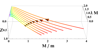
Figure 2: (color online) RG flow diagram. The starting points correspond to $Z=1$ but different values of the bare dimensionless parameters $\lambda_{0}M$ and $M/m_{0}$. The end points correspond to a line of low-energy fixed points with $Z\to 0$, $M/m\to 0$, but finite $\lambda M$.

First, we note that the quasiparticle residue $Z(\Lambda)$ decreases monotonically as we lower the energy scale. This behavior is reminiscent of another impurity model studied in condensed matter physics, namely the x-ray edge problem mahan . In the latter, the quasiparticle residue of a localized core-hole state that interacts with low-energy electron-hole pairs in a metal vanishes as a power law in the low energy limit. The power law stems from resumming logarithmic singularities such as the one that appears in Eq. (13), and is a manifestation of the orthogonality catastrophe noziere ; noziere2 ; noziere3 . Based on this observation, we expect an analogy between the x-ray edge problem and the physics of the Tkachenko polaron at low energies if we replace the core-hole by the mobile impurity and the low-energy electron-hole pairs by Tkachenko modes.

The analogy with the x-ray edge problem can be pursued further since the solution of the RG equations shows that the effective impurity mass diverges in the low-energy limit. Thus, there is a crossover from the light impurity regime, in which $m(\Lambda)\ll M$, to the heavy impurity regime, in which $m(\Lambda)\gg M$.

Furthermore, we note that the effective coupling constant $\lambda(\Lambda)$ initially grows under the RG flow, in agreement with the results in Ref. PRL111 . However, the growth is slowed down by the suppression of the quasiparticle weight $Z(\Lambda)$, which affects the vertex correction through the impurity propagators. As a result, for $\Lambda\to 0$ the effective $\lambda$ converges to a finite value $\lambda^{*}$ (see Fig. 2) that depends on the initial value of the bare coupling constant at scale $\Lambda_{0}$. Therefore, the parameters in the Tkachenko polaron model flow towards a line of fixed points with $Z=0,\tilde{m}\to\infty$ and continuously varying coupling constant $\lambda^{*}$. A similar line of fixed points is found in the Kosterlitz-Thouless flow diagram which arises for instance in the ferromagnetic regime of the anisotropic Kondo model and resonant level models anderson ; varma . Importantly, here the values of $\lambda^{*}$ are larger than the corresponding bare $\lambda(\Lambda_{0})$ only by a factor of order 1. This means that, if we start in the weak coupling regime $\lambda\mu\ll 1$ with $\mu\approx m(\Lambda_{0})$ for a light Tkachenko polaron, the renormalized coupling constant in the low energy limit may still be small according to a new criterion $\lambda^{*}\mu^{*}\ll 1$, with $\mu^{*}\approx M$ for $m(\Lambda)\gg M$. In this weak coupling regime, it is justifiable to neglect higher-order corrections in the RG equations.

Close to a fixed point with renormalized coupling constant $\lambda^{*}$ and in the regime $m(\Lambda)\gg M$, we can simplify the RG equations (16) and (18):

$$\frac{dZ}{d\ell} \approx -\frac{(\lambda^{*}M)^{2}}{\pi}Z,$$ (19)

$$\frac{d\tilde{m}}{d\ell} \approx \frac{2(\lambda^{*}M)^{2}}{\pi}.$$ (20)

The solution implies that in the low energy limit the quasiparticle weight vanishes as a power law with exponent controlled by the renormalized coupling, $Z(\Lambda)\sim(\Lambda/\Lambda_{0})^{(\lambda^{*}M)^{2}/\pi}$, whereas the renormalized mass diverges logarithmically, $\tilde{m}(\Lambda)\sim\frac{2(\lambda^{*}M)^{2}}{\pi}\ln(\Lambda_{0}/\Lambda)$.

IV Spectral function in the low energy limit

The RG analysis in the previous section suggests a simple picture for the low-energy fixed points of the Tkachenko polaron model in terms of a heavy impurity (with a logarithmically divergent effective mass) with a finite coupling $\lambda^{*}$ to low-energy Tkachenko modes. In this section we address the line shape of the single-particle spectral function at low energies, close to a heavy-impurity fixed point. We first show that, within the approximation of setting $m\to\infty$, the Hamiltonian can be diagonalized exactly and the spectral function is described by a power-law singularity with a nonuniversal exponent governed by $\lambda^{*}$. Next, we discuss an approximation to treat the effects of a large but finite impurity mass, the most important of which is to round off the singularity around the renormalized impurity dispersion.

IV.1 Dispersionless impurity

In the regime $m(\Lambda)\gg M,1/\lambda^{*}$, we start with the simplest possible approximation of neglecting the kinetic energy of the impurity in Eq. (4). In this case of infinite mass, the model is equivalent to a localized impurity coupled to bosonic modes and can be solved exactly by a unitary transformation

$$U=\exp\left[-\frac{1}{\sqrt{\mathcal{S}}}\sum_{\textbf{q}}\alpha_{q}\,(\hat{a}_{\textbf{q}}-\hat{a}_{-\textbf{q}}^{\dagger})\hat{n}_{-\mathbf{q}}\right],$$ (21)

where $\hat{n}_{\mathbf{q}}=\sum_{\mathbf{k}}\hat{b}_{\textbf{k}}^{\dagger}\hat{b}^{\phantom{\dagger}}_{\textbf{k}+\textbf{q}}$ is the Fourier transform of the impurity density operator and $\alpha_{q}$ is a real function of $q=|\mathbf{q}|$ to be specified below. Eq. (21) is analogous to the Lang-Firsov transformation used in the small polaron regime for lattice models with strong electron-phonon interaction mahan . Using the identity $e^{X}\hat{O}e^{-X}=\hat{O}+[X,\hat{O}]+\frac{1}{2!}[X,[X,\hat{O}]]+...$, we obtain the displacement of the Tkachenko boson operator

$$U^{\dagger}\hat{a}_{\mathbf{q}}U=\hat{a}_{\mathbf{q}}-\frac{\alpha_{q}}{\sqrt{\mathcal{S}}}\hat{n}_{\mathbf{q}}.$$ (22)

The transformation of the kinetic energy for Tkachenko modes yields

$$\tilde{H}_{ph} = U^{\dagger}H_{ph}U$$ (23)

$$= \sum_{\mathbf{q}}\omega_{\mathbf{q}}\hat{a}^{{\dagger}}_{\mathbf{q}}\hat{a}_{\mathbf{q}}-\frac{1}{\sqrt{\mathcal{S}}}\sum_{\mathbf{q}}\frac{\alpha_{q}q^{2}}{2M}\hat{n}_{-\mathbf{q}}(\hat{a}_{\mathbf{q}}+\hat{a}_{-\mathbf{q}}^{{\dagger}})$$

$$+\frac{1}{\mathcal{S}}\sum_{\mathbf{q}}\alpha_{q}^{2}\frac{q^{2}}{2M},$$

where we used $\hat{n}_{\mathbf{q}}\hat{n}_{-\mathbf{q}}=\sum_{\mathbf{k}}\hat{b}^{\dagger}_{\mathbf{k}}\hat{b}^{\phantom{\dagger}}_{\mathbf{k}}=1$ in the subspace with a single impurity. For the impurity-boson interaction term, we have

$$\tilde{H}_{imp-ph}=\frac{\lambda^{*}}{\sqrt{\mathcal{S}}}\sum_{\mathbf{q}}q\,\hat{n}_{-\mathbf{q}}(\hat{a}_{\mathbf{q}}+\hat{a}_{-\mathbf{q}}^{{\dagger}})-\frac{2}{\mathcal{S}}\sum_{\mathbf{q}}\,\alpha_{q}\lambda^{*}q.$$ (24)

Choosing $\alpha_{q}=\alpha/q$ with

$$\alpha=2M\lambda^{*}$$ (25)

eliminates the impurity-boson coupling in the transformed Hamiltonian:

$$\tilde{H}=U^{\dagger}HU=\sum_{\textbf{q}}\frac{q^{2}}{2M}\,\hat{a}_{\textbf{q}}^{\dagger}\,\hat{a}_{\textbf{q}}+const.$$ (26)

After the unitary transformation, the Hamiltonian is noninteracting and its ground state is a vacuum of the transformed bosonic modes in Eq. (26). The ground state $|\tilde{0}\rangle$ in the presence of the impurity is related to the original bosonic vacuum $|0\rangle$ by $|\tilde{0}\rangle=U|0\rangle$. Thus, the overlap between the ground states with or without the impurity is

$$\langle 0|\tilde{0}\rangle = \langle 0|\exp\left[-\frac{\alpha}{\sqrt{\mathcal{S}}}\sum_{\mathbf{q}}\frac{1}{q}\,(\hat{a}_{\textbf{q}}-\hat{a}_{-\textbf{q}}^{\dagger})\right]|0\rangle$$ (27)

$$= e^{-\frac{\alpha^{2}}{\mathcal{S}}\sum_{\mathbf{q}}\frac{1}{q^{2}}}.\quad$$

For a large vortex lattice, the sum can be converted into an integral $\frac{\alpha^{2}}{\mathcal{S}}\sum_{\mathbf{q}}\frac{1}{q^{2}}\rightarrow\frac{\alpha^{2}}{2\pi}\int_{q_{min}}^{\Lambda_{0}}\frac{dq}{q}$, which diverges logarithmically for $q_{min}\to 0$. We cut off the infrared divergence by setting the lower limit of integration to be $q_{min}\sim 2\pi/L$ with $L\sim\sqrt{\mathcal{S}}$ the length scale representing the system size. We then find

$$\langle 0|\tilde{0}\rangle\sim L^{-\alpha^{2}/2\pi}.$$ (28)

Thus, the overlap vanishes in the thermodynamic limit. As usual, the orthogonality catastrophe stems from the creation of a divergent number of low-energy, small-$q$ excitations — in this case the Tkachenko bosons — upon coupling the many-body system to a single impurity.

We can use the unitary transformation to calculate the impurity Green’s function

$$G(\mathbf{r},t>0)=-i\langle\hat{\psi}_{B}(\mathbf{r},t)\hat{\psi}_{B}^{\dagger}(\mathbf{0},0)\rangle,$$ (29)

where $\langle\,\rangle$ denotes the expectation value in the ground state of the system without impurities. Using the mode expansion of the impurity field operator $\hat{\psi}_{B}(\mathbf{r},t)=\frac{1}{\sqrt{\mathcal{S}}}\sum_{\mathbf{k}}e^{i\mathbf{k}.\mathbf{r}}\,\hat{b}_{\textbf{k}}(t)$, it is easy to show that

$$\tilde{\psi}_{B}(\mathbf{r},t) = U^{\dagger}\hat{\psi}_{B}(\mathbf{r},t)U=\hat{\psi}_{B}(\mathbf{r},t)\;e^{\alpha Y(\mathbf{r},t)},$$

where $Y(\mathbf{r})$ is the anti-hermitean displacement operator for Tkachenko modes

$$Y(\mathbf{r})=\frac{1}{\sqrt{\mathcal{S}}}\sum_{\mathbf{q}}\frac{e^{i\mathbf{q}\cdot\mathbf{r}}}{q}(\hat{a}_{\textbf{q}}-\hat{a}_{-\textbf{q}}^{\dagger}).$$ (30)

The impurity Green’s function becomes

$$G(\mathbf{r},t)=-i\langle\tilde{\psi}_{B}(\mathbf{r},t)\tilde{\psi}_{B}^{\dagger}(\mathbf{0},0)\rangle\langle e^{-\alpha Y(\mathbf{r},t)}e^{\alpha Y(\mathbf{0},0)}\rangle,$$ (31)

where we used the decoupling of impurity and Tkachenko modes in the transformed Hamiltonian, with $\langle\,\rangle$ the free impurity background. The field $\tilde{\psi}_{B}^{\dagger}$ creates a free impurity with infinite mass at position $\mathbf{r}$. The operator $e^{-\alpha Y(\mathbf{r})}$ can be interpreted as creating the cloud of Tkachenko bosons around the impurity. Since the problem is now noninteracting, we can calculate the exact propagators. For the impurity term we have

$$\langle\tilde{\psi}_{B}(\mathbf{r},t)\tilde{\psi}_{B}^{\dagger}(\mathbf{0},0)\rangle=\frac{1}{\mathcal{S}}\sum_{\textbf{k}}e^{i\mathbf{k}\cdot\mathbf{r}}=\delta(\mathbf{r}),$$ (32)

where we used $\varepsilon_{\mathbf{k}}=0$ for $m\to\infty$. For the bosonic part in Eq. (31) we use the Baker-Hausdorff formula $e^{A+B}=e^{A}e^{B}e^{-[A,B]/2}$ to rewrite the operators in normal order, and obtain

$$\langle e^{-\alpha Y(\mathbf{r},t)}e^{\alpha Y(\mathbf{0},0)}\rangle = e^{\alpha^{2}I(\mathbf{r},t)},$$ (33)

with $I(\mathbf{r},t)=\frac{1}{2\pi}\int\frac{dq}{q}\left[\exp(-i\omega_{q}t)J_{0}(qr)-1\right]$, where $J_{0}(x)$ is the Bessel function of the first kind. Due to the delta function at the position of the impurity in Eq. (32), we can set $\mathbf{r}=0$ in Eq. (33). For $t\gg(\Lambda_{0}^{2}/2M)^{-1}$, we have

$$I(\mathbf{r}=0,t)\approx-\frac{1}{4\pi}\left[\gamma+\ln\left(\frac{i\Lambda_{0}^{2}t}{2M}\right)\right],$$ (34)

where $\gamma$ is Euler’s constant. Substituting Eq. (34) in Eqs. (33), we obtain a power-law decay

$$\langle e^{-\alpha Y(\mathbf{0},t)}e^{\alpha Y(\mathbf{0},0)}\rangle\propto t^{-\alpha^{2}/4\pi}.$$ (35)

The Green’s function for the localized impurity is then

$$G(\mathbf{r},t)\propto\delta(\mathbf{r})\;t^{-\alpha^{2}/4\pi}.$$ (36)

The nonuniversal exponent $\alpha^{2}/4\pi=(M\lambda^{*})^{2}/\pi$ is consistent with the result for the orthogonality catastrophe in Eq. (28). The spectral function defined in Eq. (9) can be calculated by taking the Fourier transform of Eq. (36). The result is a power-law singularity

$$A(\mathbf{k},\omega)\sim\omega^{-1+\alpha^{2}/4\pi}.$$ (37)

We obtain a divergent singularity if the renormalized coupling obeys the condition $(M\lambda^{*})^{2}<\pi$, which is verified in the perturbative regime $M\lambda^{*}\ll 1$.

IV.2 Finite impurity mass

When the impurity mass $m$ is finite, the unitary transformation in Eq. (21) does not diagonalize the Hamiltonian exactly because the transformation of the impurity kinetic energy $H_{imp}$ generates additional interactions:

$$\tilde{H}_{imp} = \sum_{\mathbf{k}}\varepsilon_{\mathbf{k}}\hat{b}^{{\dagger}}_{\mathbf{k}}\hat{b}^{\phantom{\dagger}}_{\mathbf{k}}+\frac{1}{\sqrt{\mathcal{S}}}\sum_{\mathbf{q}}\alpha_{q}\hat{\mathbf{J}}_{-\mathbf{q}}\cdot\mathbf{q}(\hat{a}_{\mathbf{q}}-\hat{a}_{-\mathbf{q}}^{{\dagger}})$$ (38)

$$+\frac{1}{2\mathcal{S}}\sum_{\mathbf{q},\mathbf{q}^{\prime}}\alpha_{q}\alpha_{q^{\prime}}\frac{\mathbf{q}\cdot\mathbf{q}^{\prime}}{m}\times$$

$$\times\hat{n}_{-\mathbf{q}-\mathbf{q}^{\prime}}(\hat{a}^{\phantom{\dagger}}_{\mathbf{q}}-\hat{a}_{-\mathbf{q}}^{{\dagger}})(\hat{a}^{\phantom{\dagger}}_{\mathbf{q}^{\prime}}-\hat{a}_{-\mathbf{q}^{\prime}}^{{\dagger}}),$$

where

$$\hat{\mathbf{J}}_{\mathbf{q}}=\frac{1}{m}\sum_{\mathbf{k}}\left(\mathbf{k}+\frac{\mathbf{q}}{2}\right)\hat{b}^{{\dagger}}_{\mathbf{k}}\hat{b}^{\phantom{\dagger}}_{\mathbf{k}+\mathbf{q}}$$ (39)

is the impurity current operator.

Here we resort to a variational method based on a partial polaron transformation siebel ; agarwal . The idea is that, when the impurity mass is large compared to the Tkachenko boson mass, the bosonic field can instantaneously adjust to the slow motion of the impurity. We then employ a variational ground state which is a vacuum of bosons in the appropriate representation. In practice, we perform a unitary transformation of the form in Eq. (21) and fix the function $\alpha_{q}$ by the condition that the polaron ground state energy be minimized in a new boson vacuum $|\tilde{0}\rangle$ in the presence of the impurity. Taking the expectation value of Eqs. (38), (23) and (24) in a state with the impurity with momentum $\mathbf{k}$, we obtain the energy as a functional of $\alpha_{q}$

$$\mathcal{E}_{\mathbf{k}}(\alpha_{q}) = \frac{k^{2}}{2m}+\frac{1}{\mathcal{S}}\sum_{\mathbf{q}}\left(\frac{\alpha_{q}^{2}q^{2}}{2\mu}-\frac{2\lambda^{*}\alpha_{q}}{q}\right).$$ (40)

Minimizing the energy in Eq. (40) with respect to $\alpha_{q}$, we find

$$\alpha_{q}=2\mu\lambda^{*}/q,$$ (41)

which differs from the result in Eq. (25) for an infinite-mass impurity only in that the Tkachenko boson mass is replaced by the reduced mass $\mu$.

After the unitary transformation with $\alpha_{q}$ given in Eq. (41), the transformed Hamiltonian is still interacting,

$$\tilde{H} = \sum_{\textbf{q}}\omega_{\mathbf{q}}\hat{a}_{\textbf{q}}^{\dagger}\hat{a}^{\phantom{\dagger}}_{\textbf{q}}+\sum_{\textbf{k}}\varepsilon_{\mathbf{k}}\hat{b}_{\textbf{k}}^{\dagger}\hat{b}^{\phantom{\dagger}}_{\textbf{k}}+H_{r},$$

with the residual interactions

$$H_{r} = \frac{\lambda^{\prime}}{\sqrt{\mathcal{S}}}\sum_{\textbf{k},\textbf{q}}q\,\hat{b}_{\textbf{k}+\textbf{q}}^{\dagger}\hat{b}^{\phantom{\dagger}}_{\textbf{k}}\,(\hat{a}_{\textbf{q}}+\hat{a}_{-\textbf{q}}^{\dagger})$$ (42)

$$+\frac{2\lambda^{\prime}}{\sqrt{\mathcal{S}}}\sum_{\textbf{k},\textbf{q}}\frac{\mathbf{q}}{q}\cdot\left(\mathbf{k}-\frac{\mathbf{q}}{2}\right)\hat{b}_{\textbf{k}}^{\dagger}\hat{b}^{\phantom{\dagger}}_{\textbf{k}-\textbf{q}}\,(\hat{a}_{\textbf{q}}-\hat{a}_{-\textbf{q}}^{\dagger}).$$

Importantly, the residual interaction involves a rescaled coupling constant $\lambda^{\prime}=\lambda^{*}M/(m+M)$, which is suppressed by the renormalized mass ratio $M/m\ll 1$ at low energies. In Eq. (IV.2) we have discarded terms of order $(M\lambda^{*})^{2}$ in the perturbative regime $M\lambda^{*}\ll 1$.

If we first neglect the residual interactions of order $\lambda^{\prime}\ll\lambda^{*}$ in Eq. (IV.2), the Green’s function still factorizes as in Eq. (31). The only difference is that for a finite mass $m$ the free impurity propagator becomes

$$\langle{\tilde{\psi}_{B}}(\mathbf{r},t){\tilde{\psi}_{B}}^{\dagger}(\mathbf{0},0)\rangle=\frac{m}{2\pi it}\,e^{imr^{2}/2t}.$$ (43)

The Fourier transform of the Green’s function is

$$G(\mathbf{k},\omega)=-\int d^{2}rdt\,e^{-i\mathbf{k}\cdot\mathbf{r}+i\omega t}\,\frac{me^{imr^{2}/2t}}{2\pi t}e^{\bar{\alpha}^{2}I(\mathbf{r},t)},$$ (44)

where $\bar{\alpha}=2\mu\lambda^{*}$. For $m\gg M$, the fast spatial oscillations in the propagator (43) imply that the integral in Eq. (44) is dominated by short distances $r\lesssim\sqrt{t/m}$. This allows us to neglect the spatial dependence of $I(\mathbf{r},t)$. Physically, this means the Tkachenko mode diffuses much faster than the impurity and the dominant contribution stems from the long-time tail of $e^{\bar{\alpha}^{2}I(\mathbf{r},t)}$ near the origin. We then approximate

$$G(\mathbf{k},\omega) \approx \int dt\,e^{i\omega t}e^{\bar{\alpha}^{2}I(\mathbf{0},t)}\int d^{2}re^{-i\mathbf{k}\cdot\mathbf{r}}\,\frac{m}{2\pi it}\,e^{imr^{2}/2t}$$ (45)

$$= \int dt\,e^{i(\omega-\varepsilon_{\mathbf{k}})t}e^{\bar{\alpha}^{2}I(\mathbf{0},t)}.$$

Eq. (45) involves the Fourier transform of the power-law decaying boson cloud propagator in Eq. (35). However, the frequency dependence is shifted, and the spectral function develops a power-law singularity above the single-impurity threshold

$$A(\mathbf{k},\omega)\sim\theta(\omega-\varepsilon_{\mathbf{k}})(\omega-\varepsilon_{\mathbf{k}})^{-1+\eta},$$ (46)

where $\eta=\bar{\alpha}^{2}/4\pi$ and $\theta(x)$ is the Heaviside step function.

The vanishing of the spectral function for $\omega<\varepsilon_{\mathbf{k}}$ in Eq. (46) is an artifact of neglecting the residual interactions. In fact, kinematics implies that the support of the spectral function for any $\mathbf{k}$ must extend to arbitrarily low energies, since the impurity can always decay by emitting bosons with parabolic dispersion PRL111 . This also means that the approximate power law singularity obtained in Eq. (46) is inside a multiparticle continuum and must be broadened when we take into account the impurity decay due to the residual interactions.

Figure 3: (a) Lowest order diagram included in the approximation for the impurity Green’s function in the limit $m\gg M$. The disconnected part with multiple wiggly lines represents the boson cloud propagator. (b) and (c) Connected cloud diagrams neglected in the approximation.

To obtain the rounding of the singularity for $m/M\ll 1$, we apply perturbation theory in interactions (42) to calculate the Green’s function $G(\mathbf{r},t)=-i\langle\tilde{\psi}_{B}(\mathbf{r},t)\tilde{\psi}_{B}^{\dagger}(\mathbf{0},0)e^{-\bar{\alpha}Y(\mathbf{r},t)}e^{\bar{\alpha}Y(\mathbf{0},0)}e^{-i\int dt^{\prime}H_{r}(t^{\prime})}\rangle_{0}$. To order $(\lambda^{\prime})^{2}$, the simplest diagram has a self-energy insertion in the impurity propagator (see Fig. 3). There are, in addition, diagrams in which the impurity propagator is connected with the cloud propagator by taking contractions of the bosonic operators in $H_{r}$ with the operators $e^{\bar{\alpha}Y(\mathbf{r})}$. However, the latter type of contraction introduces an additional factor of $\bar{\alpha}^{2}\sim(\mu\lambda^{*})^{2}$. Thus, in the perturbative regime $M\lambda^{*}\ll 1$ we neglect diagrams that connect the impurity to the boson cloud propagator and sum up the series of self-energy diagrams such as the one in Fig. 3a. Within this approximation, we have $G(\mathbf{r},t)=\mathcal{G}(\mathbf{r},t)e^{\bar{\alpha}^{2}I(\mathbf{r},t)}$, where $\mathcal{G}(\mathbf{r},t)$ is the impurity Green’s function dressed with the self-energy from the residual interactions. Taking the Fourier transform of $G(\mathbf{r},t)$ and neglecting the spatial dependence of $I(\mathbf{r},t)$, we obtain

$$G(\mathbf{k},\omega)\approx\frac{2e^{-\gamma\eta}\sin(\pi\eta)\Gamma(1-\eta)}{(i\Lambda_{0}^{2}/2M)^{\eta}}\int_{\omega}^{\infty}\frac{d\omega^{\prime}}{2\pi}\frac{\mathcal{G}(\mathbf{k},\omega^{\prime})}{(\omega^{\prime}-\omega)^{1-\eta}}.$$ (47)

The dressed impurity Green’s function is

$$\mathcal{G}(\mathbf{k},\omega)=\frac{1}{\omega-\varepsilon_{\mathbf{k}}-\Sigma_{r}(\mathbf{k},\omega)}.$$ (48)

The real part of $\Sigma_{r}(\mathbf{k},\omega)$ is cutoff dependent and contains logarithmic divergences, which appear again because the residual interaction is marginal. These divergences must be absorbed in the definition of the renormalized parameters. We are mainly interested in the imaginary part

$$\mathrm{Im}\Sigma_{r}(\mathbf{k},\omega) = -(\lambda^{\prime})^{2}\left[\mu k^{2}+2m^{2}(\varepsilon_{\mathbf{k}}-\omega)\theta(\varepsilon_{\mathbf{k}}-\omega)\right]\times$$ (49)

$$\times\theta[\omega-\varepsilon_{min}(k)],$$

where $\varepsilon_{min}(k)=k^{2}/[2(m+M)]$ is the lower threshold of the two-particle (impurity plus one boson) continuum. The threshold at $\omega=\varepsilon_{min}(k)$ is an artifact of calculating $\Sigma_{r}$ only to order $(\lambda^{\prime})^{2}$. At higher orders in perturbation theory $\textrm{Im}\Sigma(\mathbf{k},\omega)$ must be nonzero for any $\omega>0$. But notice that the energy window between the two-particle lower threshold and the single-impurity energy, $\delta\varepsilon_{k}=\varepsilon_{\mathbf{k}}-\varepsilon_{min}(k)\approx Mk^{2}/m^{2}$, vanishes more rapidly than $\varepsilon_{\mathbf{k}}$ as the effective mass $m(k)$ diverges for $k\to 0$. This is expected since the phase space available for scattering decreases as the impurity becomes heavier and the recoil energy vanishes noziere . The same behavior is observed for the decay rate calculated from the residual interaction

$$\gamma^{r}_{\mathbf{k}}\approx-\textrm{Im}\Sigma_{r}(\mathbf{k},\omega=\varepsilon_{\mathbf{k}})=(\lambda^{\prime})^{2}\mu k^{2},$$ (50)

which also scales like $\sim 1/m^{2}$ for $m\gg M$.

Since we are interested in the broadening of the spectral function in a small energy window $|\omega-\varepsilon_{\mathbf{k}}|/\varepsilon_{\mathbf{k}}\sim M/m\ll 1$, we approximate $\Sigma_{r}(\mathbf{k},\omega)\approx\Sigma_{r}(\mathbf{k},\varepsilon_{\mathbf{k}})$. We absorb the real part of the self-energy into the renormalized dispersion $E_{\mathbf{k}}$ and write the imaginary part as the decay rate $\gamma^{r}_{\mathbf{k}}$. Then from Eq. (47) we obtain the result for the spectral function

$$A(\mathbf{k},\omega)\propto\frac{\sin\left\{(1-\eta)\left[\frac{\pi}{2}-\arctan\left(\frac{E_{\mathbf{k}}-\omega}{\gamma^{r}_{\mathbf{k}}}\right)\right]\right\}}{\left[(\omega-E_{\mathbf{k}})^{2}+(\gamma^{r}_{\mathbf{k}})^{2}\right]^{(1-\eta)/2}}.$$ (51)

The spectral function has a broadened peak at $\omega\approx E_{\mathbf{k}}$; but since $\gamma^{r}_{\mathbf{k}}/E_{\mathbf{k}}$ decreases as the effective impurity mass increases, the peak becomes more pronounced for smaller $k$ and we recover the power-law singularity in the limit $k\rightarrow 0$, $m\rightarrow\infty$. The change in the line shape of $A(\mathbf{k},\omega)$ between the large $k$ and small $k$ regimes is illustrated in Fig. 4.

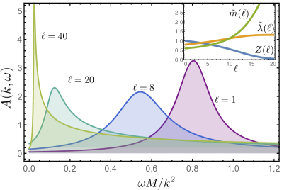
Figure 4: (color online) Impurity spectral function $A(k,\omega)$ in the low energy regime for four different values of $k=\Lambda_{0}e^{-\ell}$. As $\ell$ increases, the line shape crosses over from a Lorentzian to an approximate power-law singularity. The inset shows the RG flow of the dimensionless parameters; here we set the bare values to $Z(0)=1,\tilde{m}(0)=0.6,\tilde{\lambda}(0)=0.8$. Here we set $\Lambda_{0}=M=1$. The spectral function is normalized so as to obey the sum rule mahan $\int_{0}^{K}d\omega\,A(k,\omega)=1$, with a cutoff on the high-frequency tail of Eq. (51) set by $K=k^{2}/[M\tilde{m}(0)]$.

V Probing the excitation spectrum

Analogous to angle resolved photoemission spectroscopy (ARPES) used to measure the single-particle spectral function of electrons in metals, in cold atom setups there is the technique of momentum resolved radio-frequency (rf) spectroscopy T1 ; T2 . Basically, a rf light pulse is used to transfer impurity atoms to a hyperfine level that does not interact with the background atoms. After that, a free expansion absorption image provides the momentum distribution of the impurity sample. Since the rf pulse does not alter the original atomic momentum, one can recover the impurity single-particle spectrum combining the information from the hyperfine level separation (energy of the light pulse) and the release energy of the free expanding atoms. To probe different regimes in the spectral function, we should start with an external force that acts selectively on impurity atoms (through a magnetic field gradient shashi or a two-photon stimulated Raman transition ketterle ; berciu ) to impart a well-defined initial momentum. Then a rf pulse can be applied, after an appropriate time interval, to transfer the initially interacting impurities to a noninteracting final state. The release energy of the dilute impurity sample can be measured trough the time of flight state-selective absorption image, realized with the same holding time, but for different impurity momenta applied initially.

As in the x-ray edge problem mahan , the single-particle Green’s function in real time $G(\mathbf{k},t)$ can be related to a time-dependent overlap $\langle 0_{k}|e^{iH_{A}t}e^{-i(H_{A}+H_{B}+H_{int})t}|0_{k}\rangle$, where $|\tilde{0}_{k}\rangle=\hat{b}^{\dagger}_{\mathbf{k}}|0\rangle$. It has been proposed that this type of overlap can be measured directly using Ramsey-type interferometry PRX . In our case, measuring the decay of the overlap with time would be useful to distinguish between the two regimes in the spectral function. For momentum $l^{-1}e^{-\pi/4\mu_{0}^{2}\lambda_{0}^{2}}\ll k\ll l^{-1}$, we expect an exponential decay $\sim e^{-\gamma_{\mathbf{k}}t}$ controlled by the width $\gamma_{\mathbf{k}}$ of the Lorentzian peak in $A(\mathbf{k},\omega)$. In the long wavelength regime $k\ll l^{-1}e^{-\pi/4\mu_{0}^{2}\lambda_{0}^{2}}$ and for intermediate times $(Ml^{2})^{-1}\ll t\ll(\gamma^{r}_{\mathbf{k}})^{-1}$, one should observe a power law decay $\sim t^{-\eta}$ as a signature of the orthogonality catastrophe and breakdown of the quasiparticle picture for the Tkachenko polaron.

While we have emphasized the crossover in the spectral function as a function of momentum, the orthogonality catastrophe in the vortex lattice could also be observed using impurities localized by an external potential. In this case it would suffice to measure the frequency dependence in rf spectroscopy, removing the need for momentum resolved techniques.

VI Conclusion

We have studied the model of a neutral impurity weakly coupled with the Tkachenko modes of a vortex lattice Bose-Einstein condensate. We have described how the line shape of the impurity spectral function is modified as the impurity momentum varies between a perturbative regime $k\gg l^{-1}e^{-\pi/4\mu_{0}^{2}\lambda_{0}^{2}}$ and a low energy regime $k\ll l^{-1}e^{-\pi/4\mu_{0}^{2}\lambda_{0}^{2}}$. In the low energy limit the spectral function develops a power law singularity. The latter is a signature of the orthogonality catastrophe that arises as the effective impurity mass $m(k)$ grows with the RG flow and the heavy impurity is dressed by an increasing number of low-energy Tkachenko modes. For any $k>0$, the singularity is broadened due to the recoil of the finite mass impurity, but the singularity becomes well defined in the limit $k\to 0$. We have proposed that the crossover in the line shape of the Tkachenko polaron spectral function could be measured using momentum-resolved radio-frequency spectroscopy.

- (1) I. Bloch, J. Dalibard, W. Zwerger, Rev. Mod. Phys. 80, 885 (2008).
- (2) L. Mathey, D.-W. Wang, W. Hofstetter, M. D. Lukin, and E. Demler, Phys. Rev. Lett. 93, 120404 (2004).
- (3) F. M. Cucchietti and E. Timmermans, Phys. Rev. Lett 96, 210401 (2006).
- (4) M. Bruderer, A. Klein, S. R. Clark, and D. Jaksch, Phys. Rev. A 76, 011605 (2007).
- (5) G. Pupillo, A. Griessner, A. Micheli, M. Ortner, D.-W. Wang, and P. Zoller, Phys. Rev. Lett. 100, 050402 (2008).
- (6) A. Schirotzek, C.-H. Wu, A. Sommer, and M. W. Zwierlein, Phys. Rev. Lett. 102, 230402 (2009).
- (7) W. Casteels, J. Tempere and J. T. Devreese, Phys. Rev. A 84, 063612 (2011).
- (8) M. Koschorreck, D. Pertot, E. Vogt, B. Frohlich, M. Feld, and M. Kohl, Nature 485, 619 (2012).
- (9) C. Kohstall, M. Zaccanti, M. Jag, A. Trenkwalder, P. Massignan, G. M. Bruun, F. Schreck, and R. Grimm, Nature 485, 615-618 (2012).
- (10) F. Herrera, K. W. Madison, R. V. Krems, and M. Berciu, Phys. Rev. Lett. 110, 223002 (2013).
- (11) T. Fukuhara et al., Nat. Phys. 9, 235 (2013).
- (12) J. B. Balewski et al., Nature 502, 664 (2013).
- (13) P. Massignan, M. Zaccanti and G. M. Bruun, Rep. Prog. Phys. 77 034401 (2014).
- (14) J. T. Stewart, J. P. Gaebler and D. S. Jin, Nature 454, 744-747 (2008).
- (15) A. Shashi, F. Grusdt, D. A. Abanin, and E. Demler, Phys. Rev. A 89, 053617 (2014).
- (16) S. Nascimbène et al., Phys. Rev. Lett. 103, 170402 (2009).
- (17) M. M. Parish, Phys. Rev. A 83, 051603(R) (2011).
- (18) R. Schmidt, T. Enss, V. Pietilä, and E. Demler, Phys. Rev. A 85, 021602(R) (2012).
- (19) M. A. Caracanhas, V. S. Bagnato, and R. G. Pereira, Phys. Rev. Lett. 111, 115304 (2013).
- (20) J. R. Abo-Shaeer, C. Raman, J. M. Vogels, and W. Ketterle, Science 292, 476 (2001).
- (21) V. Schweikhard, I. Coddington, P. Engels, V. P. Mogendorff, and E. A. Cornell, Phys. Rev. Lett. 92, 040404 (2004).
- (22) T.-L. Ho, Phys. Rev. Lett. 87,060403 (2001).
- (23) E. J. Mueller and T.-L. Ho, Phys. Rev. Lett. 88, 180403 (2002).
- (24) E. B. Sonin, Rev. Mod. Phys. 59, 87 (1987).
- (25) J. Sinova, C. B. Hanna, and A. H. MacDonald, Phys. Rev. Lett. 89, 030403 (2002).
- (26) G. Baym, Phys. Rev. Lett. 91, 110402 (2003).
- (27) S. I. Matveenko, D. Kovrizhin, S. Ouvry, and G. V. Shlyapnikov, Phys. Rev. A 80, 063621 (2009).
- (28) S. I. Matveenko and G. V. Shlyapnikov, Phys. Rev. A 83, 033604 (2011).
- (29) G. D. Mahan, Many-Particle Physics Plenum, New York, 3rd (2000).
- (30) J. Gavoret, P. Nozieres, B. Roulet, and M. Combescot, J. Phys. France 30, 987 (1969).
- (31) P. Nozieres and C. T. De Dominicis, Phys. Rev. 178, 1097 (1969).
- (32) P. Nozieres, J. Phys. France 4, 1275 (1994).
- (33) J. Goold, T. Fogarty, N. Lo Gullo, M. Paternostro, and Th. Busch, Phys. Rev. A 84, 063632 (2011).
- (34) M. Knap, A. Shashi, Y. Nishida, A. Imambekov, D. A. Abanin and E. Demler, Phys. Rev. X 2, 041020 (2012).
- (35) M. Knap, D. A. Abanin and E. Demler, Phys. Rev. Lett. 111, 265302 (2013).
- (36) G. Refael and E. Demler, Phys. Rev. B 77, 144511 (2008).
- (37) A. Kantian, U. Schollwock, T. Giamarchi, Phys. Rev. Lett. 113, 070601 (2014).
- (38) N. R. Cooper, Adv. Phys. 57, 539 (2008).
- (39) J. Dalibard, F. Gerbier, G. Juzeliunas, P. Öhberg, Rev. Mod. Phys. 83, 1523 (2011).
- (40) Y.-J. Lin, R. L. Compton, K. Jiménez-García, J. V. Porto, and I. B. Spielman, Nature 462, 628 (2009).
- (41) I. B. Spielman, Phys. Rev. A 79, 063613 (2009).
- (42) N. R. Cooper, N. K. Wilkin, and J. M. F. Gunn, Phys. Rev. Lett. 87, 120405 (2001).
- (43) H. B. Nielsen and S. Chadha, Nucl. Phys. B 105, 445 (1976).
- (44) H. Watanabe and H. Murayama, Phys. Rev. Lett. 110, 181601 (2013).
- (45) R. Shankar, Rev. Mod. Phys. 66, 129 (1994).
- (46) P. W. Anderson, J. Phys. C 3, 2436 (1970).
- (47) T. Giamarchi, C.M. Varma, A.E. Ruckenstein and P. Nozieres, Phys. Rev. Lett. 70, 3967 (1993).
- (48) R. Silbey and R. A. Harris, J. Chem. Phys. 80, 2615 (1984).
- (49) K. Agarwal, I. Martin, M. D. Lukin, and E. Demler, Phys. Rev. B 87, 144201 (2013).
- (50) A. P. Chikkatur, A. Görlitz, D. M. Stamper-Kurn, S. Inouye, S. Gupta, and W. Ketterle, Phys. Rev. Lett. 85, 483 (2000).