On the Origin of a Sunquake during the 29 March 2014 X1 Flare

Abstract

Helioseismic data from the HMI instrument have revealed a sunquake associated with the X1 flare SOL2014-03-29T17:48 in active region NOAA 12017. We try to discover if acoustic-like impulses or actions of the Lorentz force caused the sunquake. We analyze spectropolarimetric data obtained with the Facility Infrared Spectrometer (FIRS) at the Dunn Solar Telescope (DST). Fortuitously the FIRS slit crossed the flare kernel close to the acoustic source, during the impulsive phase. The infrared FIRS data remain unsaturated throughout the flare. Stokes profiles of lines of Si I 1082.7 nm and He I 1083.0 nm are analyzed. At the flare footpoint, the Si I 1082.7 nm core intensity increases by a factor of several, the IR continuum increases by $4\pm 1\%$. Remarkably, the Si I core resembles the classical Ca II $K$ line’s self-reversed profile. With nLTE radiative models of H, C, Si and Fe these properties set the penetration depth of flare heating to 100 $\pm 100$ km, i.e. photospheric layers. Estimates of the non-magnetic energy flux are at least a factor of two less than the sunquake energy flux. Milne-Eddington inversions of the Si I line show that the local magnetic energy changes are also too small to drive the acoustic pulse. Our work raises several questions: Have we “missed” the signature of downward energy propagation? Is it intermittent in time and/or non-local? Does the 1-2 s photospheric radiative damping time discount compressive modes?

1 Introduction

Flares are among the most energetic phenomena in the solar system, with well-known impacts on the Earth. Beginning in the 1960s, it became clear that the only option for storing the large amount of energy for sudden release is the free energy associated with the magnetic field threading the Sun’s atmosphere. According to the standard model (Carmichael, 1964; Sturrock, 1966; Hirayama, 1974; Kopp and Pneuman, 1976), flares start by magnetic reconnection in the tenuous coronal plasma. Only here is the Alfvén speed sufficiently high to permit rapid evolution. Subsequently, downward directed energy in the forms of accelerated particles, magneto-plasma waves, radiation and thermal conduction deposit energy from above leading to bright ribbon-like structures in the chromosphere and, during strong flares, in the photosphere. Such temporarily heated structures (durations of minutes) then evaporate plasma into the corona, leading to post-flare loops that are bright in soft X rays and UV radiation on time scales of hours.

Local helioseismology has revealed flares which are accompanied by acoustic pulses (“sunquakes”) propagating below the visible surface. The mechanisms by which the flare disturbance, originating high in the solar atmosphere, couples to interior modes is not known, there being several challenges. Firstly, flares are difficult to observe, generally speaking, at both the necessarily small time and length scales associated with the initial energy release (impulsive phase). Secondly, most acoustic sources preferentially occur in the magnetically complex penumbrae of sunspots (e.g. Fletcher et al., 2011, section 3.6). Thirdly, the energy has to propagate through the 9 pressure scale heights of the poorly-constrained chromosphere. The chromosphere of active regions appears to be as complex as sunspot penumbrae (Judge, 2010). Measurements of magnetic fields there are difficult and rare (Navarro 2005a,b; Uitenbroek 2011).

Progress on sunquakes has been significant. For example, Donea and Lindsey (2005) have demonstrated that only a small fraction, $\mathrel{\hbox to0.0pt{\lower 3.7pt\hbox{$\sim$} \hss}\raise 1.7pt\hbox{$<$}}10^{-3}$ of the flare energy, is needed to trigger a seismic transient in the photosphere. How this happens it is not yet understood (see, e.g., discussions by Donea, 2011; Kosovichev, 2014). Recent space missions have vastly improved our ability to understand the evolving photospheric magnetic field, and significant steps have been taken towards understanding changing magnetic fields and flares. The lower solar atmosphere can show stepwise changes in line-of-sight (LOS) magnetic field strength (Kosovichev and Zharkova, 1999) and shear (Wang, 1992) during flares. Sudol and Harvey (2005) observed a LOS field change in 15 X-class flares with a median of 90 G. Recent observers have found photospheric field and inclination changes even during small B1 flares (Murray et al., 2012), using vector spectro-polarimetric data from the SP instrument on the Hinode spacecraft.

In this paper we relate acoustic sources found by Donea and others (2014) from data from the Helioseismic Magnetic Imager (HMI) on the Solar Dynamics Observatory (SDO) spacecraft, to measurements from the Facility Infrared Spectrometer (“FIRS” Jaeggli, 2011) at the Dunn Solar Telescope of the National Solar Observatory in Sunspot, New Mexico. Table 1 lists some properties of the flare and acoustic source from Donea and others (2014). While many acoustic sources are present on the Sun with this intensity, the spatial and temporal characteristics of this particular source mark it as generated by the flare. Changes in the thermal and magnetic structure in the atmosphere are reflected in our Stokes polarimeter data through a photospheric Si I line at 1082.7 nm and in the He I 1083.0 nm multiplet formed near the top of the chromosphere.

2 Observations

We made spectropolarimetric observations on March 29 2014 with FIRS and the Imaging BIdimensional Spectropolarimeter (IBIS) instruments at the DST. The latter will be reported elsewhere. In addition, we acquired, every 60 seconds, bursts of data in G-band (430.5 nm) and Ca II (393.3 nm) narrow band filters for speckle reconstruction, and a white light camera acquired rapid cadence images. FIRS was used in a single slit, dual-beam mode with a 40 micron wide slit, subtending an angular width of $0\farcs 30$, oriented close to the E-W line on the Sun.

The polarization modulation scheme was a four-state balanced scheme with 125 ms exposures and a full cycle of 1.2 s, with 10 such cycles co-added by the instrument at each scan position on the Sun. This relatively slow modulation, set by the need for the liquid crystal variable retarders to relax in response to voltage changes, runs the risk of encoding light variations entering the polarimeter due to residual seeing motion and/or solar evolution into systematic errors called “crosstalk” (Lites, 1987; Judge et al., 2004; Casini et al., 2012). Crosstalk appears to be important in the He I line during the flare as the tenuous chromospheric plasma radiating the helium emission evolves on timescales comparable or faster than the 1.2s modulation cycle. No evidence is seen for such crosstalk in the photospheric Si I line.

Throughout all our observations the count rate remained in the linear regime of the IR detector (below 8000 ADU). The solar image was scanned from S to N across the FIRS slit in 100 or 120 steps of $0\farcs 3$ to produce images in four spectropolarimetric states $S_{i}$ (linear combinations of $I,Q,U$ and $V$), covering a spectral range from 1081.93 to 1085.01 nm, and a spatial area of $30$″or $36\arcsec\times 75\arcsec$ for all scans reported here. The images have bin sizes of $0.3\arcsec$. Five scans of the slit across NOAA 12017 were begun at 16:29:26, 16:55:58, 17:40:06, 18:01:55, 18:30:13 UT. The seeing was good enough for the adaptive optics system (AO) to maintain a lock on the sunspot during the observing run. The peak flare emission is seen in the FIRS data during the third scan begun at 17:40:06 UT.

Figure 1 shows a G-band image with contours superposed, showing (black) the egression power from the acoustic holography reported by Donea and others (2014), and (white) the core intensity of the Si I line at 1082.7 nm. The G-band image was aligned with a continuum image from the HMI instrument on the SDO spacecraft obtained at 17:45:00 UT by eye, co-alignment uncertainties are at most one arcsecond. (The co-alignment accuracy is limited by the fact that the FIRS scan was obtained under varying seeing conditions and over a 20 minute scanning period). Black contours show the dominant local sources of power for waves traveling down into the solar interior. The white contours show the influence of heating processes from the flare on the regions of formation of the Si I line in the Sun’s atmosphere. The G-band image is a composite, speckle reconstructed image obtained at 17:46:44 UT. The image shows a diffuse brightening at these wavelengths centered near X=522, Y=260, which is real flare emission, with an amplitude of $\approx 1.2-1.4$ times the non-flaring intensity, perhaps a component of the still poorly understood white light emission. None of these data are strictly contemporaneous, the FIRS data shown were built of a raster scan that began at Y=254.5 at time 17:40:12 UT, and ended at Y=284.2 at 18:01:39 UT. The horizontal dashed lines show the positions of the FIRS slit at 17:45 and 17:50 UT.

2.1 Data Reduction

The FIRS data were reduced using software originally developed by Jaeggli (2011) and modified by Tom Schad (private communication 2013). The reductions followed standard procedures: correction for detector non-linearities; subtraction of dark frames; division by flat fields; co-registration of the two beams (including corrections for image rotation); polarization calibration; de-modulation (conversion of linear combinations of Stokes parameters to individual Stokes parameters). Since the required polarization sensitivity is very high in chromospheric lines (e.g. Uitenbroek, 2011), special care is needed in handling calibrations. Usual dark frames and flat fields were acquired, and a gain linearization correction was applied to the data using a curve from Jaeggli (2011). We used flats obtained with a calibration lamp which is vignetted across the detector frame, in preference to solar flats in which photospheric spectral lines are always present. This is because we analyze below the detailed profiles of the Si I line at 1082.7 nm.

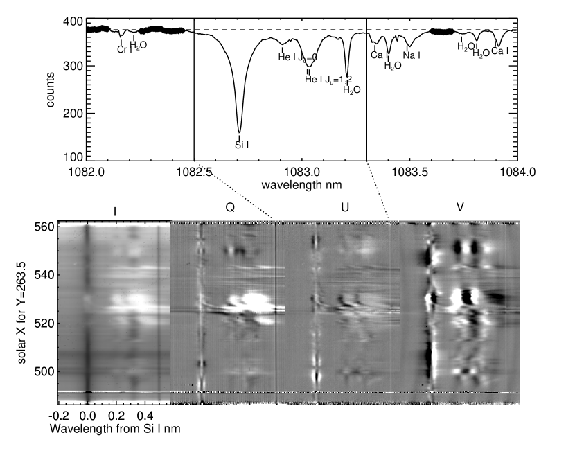
Figure 2: The upper panel shows the median intensity spectrum from the spectral scan obtained by FIRS started at 17:40:06 UT. Line identifications are marked, the ${\rm H_{2}O}$ features are all telluric and should be polarization-free. Those wavelengths used to derive the continuum intensity are marked on the spectrum with symbols. The four lower panels show Stokes $I,Q,U$ and $V$ spectra taken from the 30th scan obtained through the flare footpoint beginning at 17:46:29 UT, as a function of wavelength and position on the Sun. The dotted lines show the wavelengths plotted on the $U$ image. The images for the $QUV$ images are clipped at $\pm 2\times 10^{-2}I_{C}$. The Si I line is in emission near $X\approx 530$. The $QUV$ profiles of this line are as expected from Zeeman-induced polarization, even when the line is in emission. The He I $QU$ and $V$ profiles are peculiar and to some degree reflect the systematic errors of “crosstalk” ($QU$ have some characteristics of $I$ and $V$). Some spectral fringes are visible, particularly in the $Q$ and $V$ images.

Residual fringes and some detector artifacts are present in these data. Fringes are a source of systematic error. Using careful corrections for flat fields we have reduced fringing to $\mathrel{\hbox to0.0pt{\lower 3.7pt\hbox{$\sim$} \hss}\raise 1.7pt\hbox{$<$}}2\times 10^{-3}I_{c}$ (peak-to-trough) where $I_{C}$ is the continuum intensity, which is defined using wavelengths for each individual scan shown in Figure 2. The wavelength scales of the spectra are determined using solar flat-field scans and solar photospheric absorption lines. The spectrograph was stable at the level of 0.2 pixels in wavelength (0.004 nm) during the observations, equivalent to a Doppler shift of 0.2  km s^-1.

It is important to note that at infrared wavelengths, the enhancement of intensity during flares is moderate, quite unlike the well-known enormous UV and X-ray enhancements. All of the FIRS data were obtained in the linear regime.

2.2 Stokes line profiles

Figure 2 shows the mean intensity spectrum with annotated spectral features and, in the lower panels, Stokes profiles for $I,Q,U$ and $V$ from left to right. The particular data shown in the lower panels are from the 29th scan obtained through the flare footpoint beginning at 17:46:29 UT, just as the flare was in the impulsive phase as found from RHESSI data analysis (Donea and others, 2014). The line profiles of the photospheric Si I line are essentially consistent with polarization induced by the Zeeman effect, with the possible exception of those seen in the flare kernel. On the other hand, while the He I linear polarization ($Q,U$) profiles might initially appear to be of solar origin, the result of atomic alignment, the presence of linear polarization in the $J=0$ upper level to $J=1$ lower level transition at 1082.9 nm must be due to systematic errors. No atomic alignment is possible with these quantum numbers, nor is it possible for levels involving hyperfine structure of any ³He nuclei that might be present.

In our figures, all data are taken from the dual-beam system, but we also examined single-beam data. The signals in the two beams are very similar for all wavelengths outside of the helium lines, but that significant differences are present in the polarized helium profiles. This is a clear sign of $I-(QUV)$ crosstalk in the helium lines. The dual-beam corrections are clearly doing an excellent job at other wavelengths (for example, those in the Si I line core). We surmise that the helium lines are evolving in intensity at least as rapidly as the 1.2 s cadence of the modulation cycle, at the level of a few percent, thereby producing spurious signals. Faster modulation seems appropriate for flare observations of the chromosphere. We defer further analysis of the flare kernel data for He I to later work.

The noise levels of these Stokes $Q,U,V$ data are close to $8\times 10^{-4}I_{C}$. The largest fringes remaining are in Stokes $V$ at the level of $2\times 10^{-3}I_{C}$. The noise levels are more than adequate for us to attempt inversions of the Si I line data.

2.3 Quick look parameters

We used the Stokes profiles to derive several simpler quantities. From Stokes $I$ (intensity), we compute the $n=0,1,2$ moments $M^{(n)}$ of the line profiles weighted by wavelength from line center. We define the continuum-subtracted line intensity as

$$I^{\prime}_{x}=I_{C}-I_{x},$$

where the Doppler shift $x$ is defined as $c(\lambda/\lambda_{LAB}-1)$ with $c$ in  km s^-1. Then we define

$$M^{(n)}=\int I^{\prime}_{x}x^{n}dx.$$

The “Doppler shift” of the line is $v=M^{(1)}/M^{(0)}$  km s^-1, the line width (not shown here) is $w=\sqrt{M^{(2)}/M^{(0)}}$  km s^-1. We also computed “quick-look” quantities from the $IQUV$ Stokes parameters. These include a LOS “magnetogram” which is simply the median of the ratio of Stokes $V$ to the first derivative of Stokes $I$ with respect to wavelength over wavelengths of significant line absorption or emission. The other magnetic parameter is the field “azimuth” which is $\frac{1}{2}\arctan(U/Q)$ where again median values of the ratio $U/Q$ are taken across both the Si I line and He I multiplet. The relationship of these quantities to physical parameters in the Sun arises only when the polarization is dominated by the Zeeman effect (see, e.g. Jefferies et al., 1989) and only when the polarization $Q^{2}+U^{2}+V^{2}\ll 1$, and when the Stokes profiles all originate from the same physical volumes underlying a given pixel. Nevertheless, such quantities as LOS magnetograms are very familiar to solar physicists which, with care, illustrate properties of the solar magnetic field.

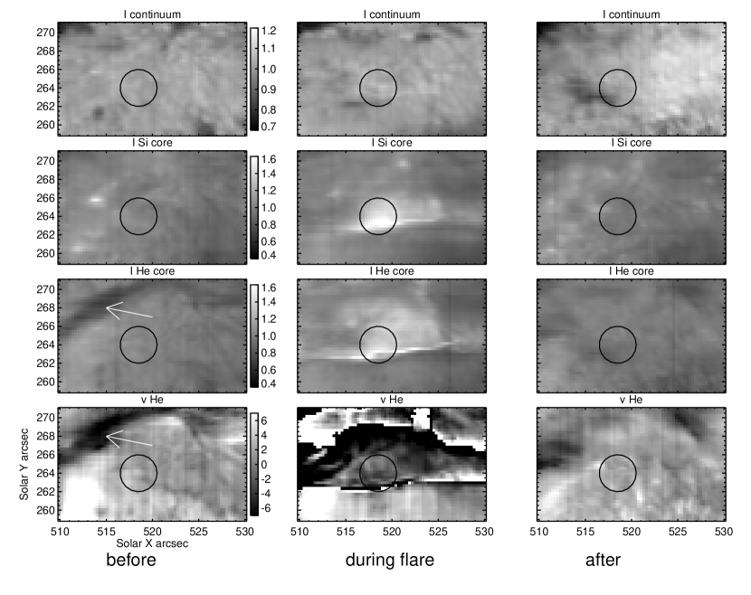
Figure 3: “Quick-look” raster images of thermal data obtained using the FIRS instrument. The columns, from left to right, show data from 16:29:26, 17:40:06 (during the impulsive phase of the flare) and 18:30:13 respectively. The top panels show continuum intensity averaged over 30 pixels on the blue side of the Si I 1028.7 nm line. The next two rows shows the intensity at the cores of the Si I and He I 1083.0 nm lines. Row 4 shows Doppler shifts of the He I multiplet in units of  km s^-1. The flare began around 17:45 UT, at about the time the FIRS slit crossed the flare ribbon seen in the Si I and He I core intensities (middle column, refer also to Figure 1). The circle shows the location of the “acoustic source” associated with the flare in the field of view shown. The arrows mark the erupting filament seen in He I.

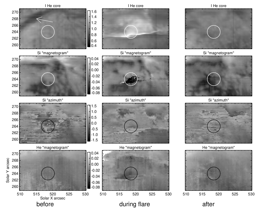
Figure 4: Quick-look raster images relevant to magnetic fields obtained using the FIRS instrument. The top panels show the intensity near the core of the He I 1083.0 nm lines from Figure 3. Rows 2 and 3 show “magnetograms” and “azimuths” of the magnetic field (see text), of the Si I line. Rows 4 and 5 show similar data but for the He I multiplet. Care should be taken not to interpret the crude magnetic data in terms of magnetic field especially during the flare, which occurred during the scan shown in the second column.

Figures 3 and  4 show some of the quick look parameters and continuum intensity from the three scans obtained before, during and after the impulsive phase. These we label phases “bef”,“dur” and “aft”. The white contours of Figure 1 are from the Si core data shown in the second row of Figure 3. Figure 4 shows parameters related to the magnetic field. Salient features of these plots include:

• The IR continuum shows only a weak brightening during scan “dur”.

• Both the photospheric Si I and chromospheric He I lines show considerable brightening during scan “dur”, in the line cores.

• The filament seen in the He I line core images, lying roughly along the neutral line seen in “bef” scan magnetograms, disappears by scan “aft”.

• The He I absorbers in the filament are seen moving upwards by between 5 and 10  km s^-1 in scan “bef”. During scan “aft”, the filament is replaced by a diffuse region of He I line absorption.

• Magnetograms show only subtle changes from scans “bef” to “dur” and “aft”.

• The photospheric magnetic azimuthal angles show systematic changes as the flare progresses.

• The He I $U/Q$ signals during scan “dur” have coherent structure whose origin includes at least some $I\rightarrow(QU)$ crosstalk. The spectral profiles show that they certainly cannot be interpreted as a traditional Zeeman-induced linear polarization.

During scan “dur” (the impulsive phase), magnetic quick-look data for the He I line cannot be trusted to represent magnetic fields because of cross-talk. We will attempt to correct for this crosstalk in a future publication, since even in the presence of atomic polarization, the 1083 nm multiplet still retains accurate information on field azimuthal angles, for field strengths $>10$G (the strong field limit of the Hanle effect). To quantify the magnetic field changes we turn to inversions for the Si I $IQUV$ data.

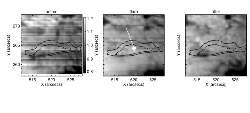
Figure 5: Continuum intensity data are shown from the three scans immediately before, during and after the X1 flare impulsive phase. The contours show the intensity from the core of the Si I line. Enhanced intensity in the continuum is seen as the central part of one row in the image the middle panel, marked by an arrow. Its amplitude is $4\pm 1\%$ of the neighboring intensities.

First we will use properties of the Si I line and continuum to constrain the depth of penetration of flare energy that is sufficient to change the temperature structure in the deep chromosphere and photosphere. At a first glance the continuum intensity appears to change very little, if at all. But both p modes and granulation modify the continuum intensity at a level of a few percent at angular resolutions similar to those of FIRS (e.g. Sánchez Cuberes et al., 2000), making relatively small changes difficult to see in slit rasters. Careful examination of the FIRS spectra obtained beginning at 17:46:16 UT, show a significant brightening of $4\pm 1$% above levels in the neighboring spectra taken 13 seconds before and after, close to the flare kernel observed in RHESSI and line data. Evidence for this is shown in Figure 5. These data include variations in the transparency and seeing conditions of the atmosphere and hence vary significantly from row to row in the figure. As is obvious in the figure, transparency variations were strongest in the first scan, getting progressively weaker in the second and third scans. However, relative intensities along each row in each panel can be fairly compared. The uncertainty quoted above is a $1\sigma$ statistical variation of the detrended intensity measured along the rows immediately adjacent to the row containing the flare.

The coherent streak of brightness in continuum data from 17:46:16 has all the characteristics of a genuine brightness increase associated with a white light flare. This picture is supported by HMI continuum data from the SDO spacecraft, which shows a $\approx$5% increase in continuum intensity during the flare. Its appearance only in one FIRS scan indicates a very rapid evolution, characteristic of an origin from dense photospheric material which has a radiative relaxation time of 1-2 seconds (Spiegel, 1957).

3 Analysis

The spatio-temporal behavior of the flare as obtained by FIRS is summarized in Figures 3 and  4. Remarkably, the slit happened to scan across the flare footpoint ribbons at the flare peak, 17:46 UT (Table 1). Also shown on the figure is the core of the flare-related acoustic source (Donea and others, 2014). It is clear that FIRS managed to capture those locations in solar-$y$ heliographic coordinate that correspond to the time and place of the acoustic source.

3.1 Helioseismic holography

Seismic transients from solar flares can be detected by pre-processing solar data and applying the analytical technique of helioseismic holography to Doppler measurement of the active region hosting the solar flare. Donea and others (2014) analyzed Doppler maps from the Helioseismic and Magnetic Imager instrument (HMI; Schou et al., 2012) on board the Solar Dynamics Observatory satellite (SDO). HMI measures properties of photospheric dynamics and magnetic fields every 45 seconds. Donea and others (2014) generated Postel projection maps of the seismic emission of NOAA 12017. We refer discussion of the principles of seismic holography to Section 4 of Lindsey and Braun (2000), with application to flare observations to Donea et al. (1999). Briefly, the seismic responses to the flare perturbations are identified through an excess of the emission power, $|H_{+}(r,t)|^{2}$. Each pixel in an image of $|H_{+}(r,t)|^{2}$ is a representation of the coherent acoustic power for waves that have propagated downward from the focus, traveled thousands of kilometers beneath the solar surface, and re-emerged into a pupil a significant distance from the focus. With this technique Donea and others (2014) uncovered a weak but significant seismic source at the footpoint shown in Figure 1. Hard X-ray emission, magnetic transients and strong UV footpoint emission were analyzed by Donea and others (2014), confirming that the seismic source is indeed associated with the flare.

3.2 The depth of penetration of flare energy

By comparing the brightness of models of continuum and Si I 1082.7 nm line to observations, we can in principle constrain the depth in the atmosphere to which significant heating from above can penetrate. Our approach is simple. We ask: what are the deepest and shallowest layers in the atmosphere heated by the flare that are compatible with the data?

To preface the model calculations below, we note that the flare Si I profile (Figure 2) resembles classical Ca II $H$ and $K$ self-reversed profiles (Linsky and Avrett, 1970), but with far weaker line absorption wings. The Ca II line cores, much more opaque than the line of silicon, form in the chromosphere with a source function dominated by scattering. The simple observation of a self-reversed profile of Si I implies a significant column mass, much higher than that for the calcium line. The breadth of a Doppler-broadened, self-reversed line is larger than an optically thin line formed under the same conditions by the factor $\approx\sqrt{\ln\tau_{0}}$ where $\tau_{0}$ is the line center optical depth. For $\tau_{0}=100$ this factor is over 2.1. The self-reversal is also very narrow (FWHM $\approx 0.015$ nm, see Figure 2), indicating turbulent speeds of FWHM/1.66 $\approx 2.5$  km s^-1 where the line core forms. A profile averaged along the region with obvious Si I emission in Figure 2 is shown in Figure 6. The averaging washes out the self-reversal in the latter plot.

We model the Si I line and the neighboring IR continuum both during and outside of the impulsive phase. We performed nLTE radiative transfer calculations, in several 1D models of the solar atmosphere, following the tradition of Vernazza et al. (1973, 1976, 1981, henceforth VAL81). We solved nLTE statistical equilibrium equations for atoms of H, C, Si and Fe using the program RH (Uitenbroek, 2000). These atoms were chosen because UV radiation controlling the Si I spectral line at 1082.7 nm is dependent on the nLTE solutions of these abundant elements. We considered using one of several flare models (e.g. Machado et al., 1989). However, these models were constructed to try to identify the origin of white light emission in flares. Our goal is different, to try to see if modeling can provide a depth of penetration of flare energy into the photosphere. Therefore we adopted a different, more straightforward strategy. We started with the model “C” of VAL81 and explored the effects of introducing temperatures plateaus of the form

$$T_{e}=T_{0}-T^{\prime}_{1}\log m,\ \ \ m_{2}>m,$$

where $m$ is the column mass of the atmosphere, $T_{0},T^{\prime}_{1}$ are non-negative constants, and $m_{2}$ is a column mass above which temperatures are changed. We have three free parameters, and so our results will not be unique. But such plateaus, with small gradients $T^{\prime}_{1}$, have justification at least during some phases of flaring plasmas seen in radiation hydrodynamic calculations (see the 50s panel of Figure 3 of Allred et al., 2005, for example). The main sensitivity of the emerging spectra is to the two parameters $a$ and $m_{2}$. Given an estimate of $m_{2}$ the height of the energy penetration follows from the $m(z)$ relationship for the model.

We made calculations in two limits: in the calculations shown in the Figures below we allowed the atmosphere to relax to a state of hydrostatic equilibrium; in the other limit we merely solved the statistical equilibrium equations with no such adjustment. The sound crossing time of the photosphere is on the order of a few scale heights divided by 7  km s^-1, a minute or so, comparable to the duration of the flare impulsive phase. These limits probably span the behavior of intensities from an evolving atmosphere. The differences between the calculations are small in photospheric layers but are significant for regions and spectra formed above 600 km above the photosphere. Such differences do not affect our conclusions which depend only on the photospheric Si I line.

These calculations are not state-of-the art in terms of dynamics, our focus is instead on a careful treatment of the formation of the Si I 1082.7 nm line and of the continua formed between 125 and 180 nm for later comparisons with SDO/AIA data. We therefore took care to use modern and complete atomic data for the Si and Fe neutrals. We used atomic energy levels and transition probabilities from NIST up to and including the $4p$ levels in Si, and we used photoionization cross sections from the OPACITY project (Seaton, 1987), treated as outlined in Judge (2007). Collisions with electrons were treated using the impact approximation for permitted transitions (Seaton, 1962), Seaton’s semi empirical formula for direct ionization (Allen, 1973), and a collision strength of 0.1 for forbidden transitions.

Figure 6 shows, in the right panels, computed and observed profiles of Si I 1082.7 nm, with all intensities normalized to quiet Sun values. These calculations are representative of two limits of the value of $m_{2}$ – and hence height of penetration – used in the models.

The first class (upper panel) allows penetration of energy and enhanced temperatures down to photospheric layers - we allowed temperatures to rise down to 0 km height by adding various plateaus at such depths. Remarkably, the model shown produces an acceptable match to the observed profiles and continuum (the He I line is not modeled here). Exploring different temperature plateaus we determined that a reasonable agreement with the line and continuum observations requires the flare energy to penetrate and heat down to a height of $\mathrel{\hbox to0.0pt{\lower 3.7pt\hbox{$\sim$} \hss}\raise 1.7pt\hbox{$>$}}100\pm 100$ km above the photosphere. The “error bar” comes from the need to produce the $4\%$ enhancement in continuum emission ($<200$ km) with temperatures that can match the Si I profile, both features spanning the region between 0 and 700 km.

The second limiting case is one where flare energy penetrates only to the mid-upper chromosphere. Downward propagating radiation enhances the cores of lines, a typical calculation is shown in the lower panels. The line width is very narrow even though we adopted non-thermal speeds (microturbulence) of up to 8 km/s in the middle chromosphere (close to the sound speed). The continuum, formed predominantly in the photosphere with a tiny contribution from optically thin emission in the plateau, is close to the pre-flare level. The computed continuum includes thermal photospheric emission as well as hydrogen recombination from the plateaus. These two contributions have been discussed by Machado et al. (1989); Kerr and Fletcher (2014), among others. The contribution from the latter is small in our calculations, the Balmer continuum originating from an optically thick layer near 350 km and the longer-wavelength ($>364$ nm) H^- and Paschen continua near 0 km.

The core of the Si I line during the flare is broad compared with a thermal width near 1.8  km s^-1 (Figure 6), and like the well-studied Ca II $H$ and $K$ lines the origin of this width appears most naturally explained through scattering (see above). Some decades ago there was a discussion of the Wilson-Bappu effect, an empirical relationship between the width of the core of the Ca II lines and stellar luminosity, in favor of line formation in terms of scattering (Ayres, 1979) and not optically thin micro- or macro-turbulence (Fosbury, 1973). The presence of the narrow self-reversed core seems irrefutable evidence for the presence of scattering and argues strongly for a deep formation of the core. Only calculations of penetration of flare energy to the photosphere produce lines broadened by scattering and self-reversals, the latter happen to be weak in the case shown in Figure 6, but not in obvious disagreement with the observed profile.

We stress that the detailed structure of our calculations is not unique and should only be viewed as an attempt to find the depth of penetration of significant heating during the impulsive phase of the flare. Overall, our comparisons with observations of the Si I 1082.7 nm line, and taking into consideration the difficulties of tying down the continuum intensity during the flare, we conclude that heating sufficient to change detectably the photospheric temperature occurs at least to about 100 $\pm 100$ km above the visible photosphere. Based on an exploration of values of $T_{0},m_{2}$ in our model, we believe that this aspect of our calculations is robust.

3.3 Inversions

We used the code MELANIE (Socas-Navarro, 2003) to invert the Si I Stokes $IQUV$ profiles to derive the vector magnetic field in the photosphere. This was done only for scans obtained before and after the impulsive phase. Codes exist for inversion of the He I multiplet (e.g. López Ariste and Casini, 2002; Lagg et al., 2004; Asensio Ramos et al., 2008), but we have not attempted such inversions yet because we must deal with significant crosstalk in the He I $QU$ profiles during the flare, and because outside of the flare these profiles are mostly of low signal-to-noise ratio.

The observed Si I line – $3p4s~{}^{3}\!P^{o}_{2}-3p4p~{}^{3}\!P^{e}_{2}$ (lower and upper levels respectively) – forms between $\approx$ 100 km (wings) and 600 km (core) above the photosphere in our 1D models. MELANIE solves for a solution to the Milne-Eddington equations (source function linear with optical depth) for lines with Zeeman-induced polarization, minimizing differences between observed and computed profiles. The solution includes the vector magnetic field (with its 180^∘ ambiguity), opacity, Doppler width and shift, damping parameter, non-magnetic filling factor. The Milne-Eddington approximation is a simplification that surely is invalid during the flare itself. But before and after the flare its use appears reasonable, outside of bright flare ribbons and below say 600 km in the atmosphere. Our conclusions will be based only on the non-flaring atmosphere.

We inverted all five scans. We set the statistical uncertainty of each data point to $10^{-3}I_{C}$ to evaluate values of $\chi^{2}$, estimated using the measured fluctuations in $QUV$ at typical continuum wavelengths. For comparison, some of the best vector polarimetric data, the “deep mode high S/N” observations from the SP instrument on the Hinode spacecraft have rms noise of $3\times 10^{-4}I_{C}$ in the 630 nm region, for integrations of 67 s (Lites et al., 2008). Outside of the flare scan, the distribution of $\chi^{2}$ peaks near 40, showing that systematic errors are large and/or the model parameterization is poor. Given the residual fringing and other artifacts evident in the data, this does not by necessity imply that the model is poor. The reproducibility of the inversions was tested by initializing the same dataset with two different random initial guesses. The resulting rms variations in the magnetic field strength $B$ are 140 G, inclination 18^∘, azimuth $41^{\circ}$, and the LOS $B$ 30 G.

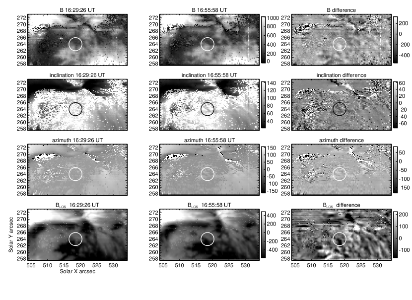
Figure 7: Magnetic field properties determined from the scans obtained before the flare, begun at 16:29:26 and 16:55:58 UT, using the code MELANIE. The azimuth is measured in the E-W direction, the sign of the azimuth is not determined. The angles are measured in the local solar frame (E-W and local vertical reference directions). The circle shows the center of the acoustic source. The rightmost column shows differenced data.

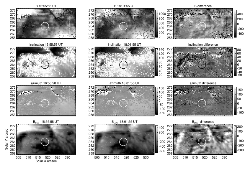
Figure 8: Magnetic field properties determined from the scans obtained before (16:55:58 UT) and after (18:01:55 UT) the flare, shown as in Figure 7.

Figures 7 and 8 show results of inversions of the scans obtained before and after the flare, begun at 16:29:26, 16:55:58, and 18:01:55 UT. No attempt at a resolution of the 180^∘ ambiguity in the field azimuth has been made, and the angles are defined relative to the local vertical (inclination) and in the plane of sky (azimuth, zero and $180^{\circ}$ being along the E-W direction). Circles show the location of the center of the acoustic source. Figure 7 shows measured changes in magnetic parameters in the two scans obtained before the flare. There are detectable differences across the bulk of the field of view in all magnetic parameters. Focusing on data in the circled region of the acoustic source, we see a significant increase in the field strength in this region, accompanied by becoming more inclined to the vertical direction (data shown in the first two rows of the Figure). Note that the circled region is some 5$\arcsec$ from the polarity inversion line. The maps of $B$ suggest that a channel of weak field is moved to the west by an arcsecond. Initially the field is inclined at some 130^∘ to the vertical. But by 17:05 UT two bands of field connected in a “Y-shape” on its side in the image appear more inclined to the vertical. The field azimuth in the “Y” shape departs significantly from initially E-W to more N-S. The LOS field within at the circle’s center shows an increase that results from increases in $B$ despite the decrease in inclination. It is unclear from our data if these changing fields arise from motions of field vertically (flux emergence) or horizontally (flows). There is little evidence for vertical motions from the LOS velocity measurements shown in Figure 3, but the inversion data (not shown) reveal a very small (-0.3  km s^-1) blue-shift pattern in the Si I data in the 10:55:58 UT scan that might conceivably be associated with the upper part only of the “Y” pattern seen in the magnetic data.

The scans upon which the inversions are based are 26 minutes apart. The above changes are unremarkable when compared to the larger field of view, except that they are within the circle encompassing the acoustic source and they are significant in all magnetic parameters.

Figure 8 shows measured changes before and after the flare itself, scans begun 66 minutes apart. The difference panels show again an increase of $B$ and azimuth, and a weak reduction of inclination, in a band in the E-W direction cutting through the circled region, flanked by regions of increased inclination just to the S and N. This sheared region (differentially changing field inclinations with time) appears aligned with the bright footpoint emission seen in the core intensities of the Si I and He I lines. The data are noisy, however.

Thus, our analysis hints that magnetic fields associated with the particular acoustic source evolve to become more sheared (i.e. inclination angles diverging in time), stronger (perhaps due to flux emergence) and rotated relative to the EW direction, during the flare. These results appear to correspond to a mixture of earlier results. Wang et al. (2012a) found penumbral fields which became more vertical after flaring. In contrast, for some flares Martínez-Oliveros et al. (2008); Wang et al. (2012b) reported field lines highly inclined to the vertical after a flare-associated seismic transient. We note that the seismic source we have analyzed is unusual. It is found near a magnetic pore, emerging from a magnetically quieter area somewhere between the main two sunspots of the AR12017 (Donea and others, 2014), instead of in a penumbra.

Lastly, if flux emergence were responsible for these measured changes in magnetic field, in 1 hour the plasma and magnetic field moving vertically through the compressible sub-photosphere with a surface velocity $\mathrel{\hbox to0.0pt{\lower 3.7pt\hbox{$\sim$} \hss}\raise 1.7pt\hbox{$<$}}0.3$  km s^-1 could have emerged from depths no deeper than $\approx 200$ km. If advected by granules with 1  km s^-1 speeds, the flux could have emerged from no deeper than 600km. It is interesting to consider how such changes to the immediate subsurface structure might or might not affect the generation of sunquakes.

3.4 The mode of transfer of flare energy down through the atmosphere

Armed with a unique dataset, we have studied the depth of penetration of flare energy down into the solar photosphere. We have shown that the detected changes in thermal structure in the atmosphere reach the photospheric level, but barely. Here we examine possible modes by which the energy might be transported through the photosphere into the deeper solar layers, thereby exciting the sunquake.

The power in the main kernel of the acoustic source measured using seismology from HMI is (Donea and others, 2014):

$$P=1.3\pm 0.05\times 10^{26}{\rm erg~{}s^{-1}}.$$

This power is distributed over an area including the main kernel centered at $(X,Y)=(518,264)$ (see Figure 1), the source just to the SW requiring an additional $1.0\times 10^{26}$ erg s^-1. The main source’s spatial distribution is nearly bi-Gaussian with a geometric mean full width at half-maximum (FWHM) of $w=4.2$ HMI pixels, $w\equiv 1.5\times 10^{8}$ cm. The peak of the power per unit area is $F=P/(A=\pi a^{2})$ with $a=w/2\sqrt{\ln 2}$, or

$$F=5\times 10^{9}{\rm erg~{}cm^{-2}~{}s^{-1}}.$$

This should be regarded as a lower limit since both the holographic technique and HMI have non-negligible angular resolutions. The area $A=2.6\times 10^{16}$ cm² is strictly an upper limit for the same reasons.

Let us consider first “non-magnetic mechanisms” by which energy is transported to the acoustic source. In this picture the changing magnetic field generates thermal perturbations indirectly via the end product of large coronal magnetic restructuring (conduction, particles, local downward radiative heating), channeling some flare energy into the photosphere. We can estimate energy fluxes into the acoustic source region that are compatible with our observations in several ways. First, we note that the excess thermal energy radiated from the photosphere during the few minutes of the rise phase is roughly 4-5% (i.e. the measured continuum enhancement) of the unperturbed solar radiative flux density $F_{\odot}=6.33\times 10^{10}$  ergs cm${}^{-2}\,$s^-1:

$$P_{RAD}\approx 0.04F_{\odot}A\mathrel{\hbox to0.0pt{\lower 3.7pt\hbox{$\sim$} \hss}\raise 1.7pt\hbox{$<$}}7\times 10^{25}{\rm\ erg~{}s^{-1}}.$$

The radiative cooling time of photospheric plasma is 1-2 s (Spiegel, 1957). Curiously then, although $P_{RAD}\sim P$, this excess thermal energy is simply radiated into space on such timescales, and is unavailable to contribute to $P$. We can look at the enthalpy flux $F_{enth}$ associated with bulk flows into the photosphere, for this we need a measurement of plasma motions and we turn to the Si I line core emission which forms between 200 and 500 km in our models. We use pressures $p=2\times 10^{4}$ dyne cm^-2 and densities $\rho=4\times 10^{-8}$ g cm^-2. corresponding to 300 km height. These are conservatively high values for average thermal properties of the plasma where this line is formed, favoring higher estimates of energy transport.

A careful comparison of the flare emission core and the pre-flare absorption profile of the Si I line reveals an upper limit to differential flows of roughly 0.5 wavelength pixels, 0.5  km s^-1. This is equivalent to 2.5$\sigma$ where $\sigma$ is the sensitivity of the Doppler shifts from our FIRS spectra. A Doppler photospheric signature of the flare is present in HMI data at the location of the seismic source with a shift equivalent to $u\approx 0.3-0.5$  km s^-1 (Donea and others, 2014). However, such filtergram data, scanning wavelengths in time, cannot be trusted during flaring and so we adopt the upper limit above. We then find an upper limit to the enthalpy energy flux of

$$F_{enth}\mathrel{\hbox to0.0pt{\lower 3.7pt\hbox{$\sim$} \hss}\raise 1.7pt\hbox{$<$}}\,\frac{5}{2}p\,u\,A\approx 6\times 10^{25}{\rm erg~{}s^{-1}}.$$

The close agreement of the upper limit for $F_{enth}$ with $F_{rad}$ means that the excess energy radiated by the photosphere during the flare can be supplied by a bulk flow of energy associated with a subsonic downflow of 0.5  km s^-1 induced (somehow) by the flare. The power in the acoustic pulse is a factor of at least 2 larger than our optimistic estimate of $F_{enth}$.

If however the pressure pulse involves high frequency phenomena ($\nu>c_{S}/H\approx 60$ mHz, where $H$ is the pressure scale height and $c_{S}$ the sound speed), the pulse would be invisible to observation except as a broadening of spectral lines to at most the sound speed (for linear waves), the lines being formed over a length $\approx H$ in a stratified atmosphere. The WKB expression for the energy flux density (propagating both upwards and downwards) at the sound speed is

$$F_{wave}=\rho c_{S}\langle\xi^{2}\rangle\ \ \ {\rm erg~{}cm^{-2}s^{-1}},$$

where $\xi$ is the velocity amplitude of the wave. We can set limits on $\xi$ through the measured line broadening and line profiles during the flare itself. Before and after the flare, the inversions yield $\xi\mathrel{\hbox to0.0pt{\lower 3.7pt\hbox{$\sim$} \hss}\raise 1.7pt\hbox{$<$}}2.8$  km s^-1. During the flare the measured line wings are similar in shape to the pre- and post- flare profiles. The emission core of the profile has a FWHM of 0.05 nm (Figures 2 and 6). Treated as optically thin emission, this FWHM is equivalent to an e-folding Doppler broadening speed of $8$  km s^-1. In the presence of scattering this is a strict upper limit. To estimate the energy flux available in such modes we again use $\rho=4\times 10^{-8}$ g cm^-2, and the upper limit of 8  km s^-1. Assuming that only half of the waves are emitted downwards, we find

$$F_{wave}A\mathrel{\hbox to0.0pt{\lower 3.7pt\hbox{$\sim$} \hss}\raise 1.7pt\hbox{$<$}}2.5\times 10^{26}\ \ {\rm erg~{}s^{-1}}.$$

But this, we believe, is a gross over-estimate. Firstly, the scattering leads to emission profiles a factor of $\approx\sqrt{\ln\tau_{0}}$ broader than mere Doppler broadening where $\tau_{0}$ is the line center optical depth. We are able to reproduce the core Si I emission using microturbulent speeds of 1-2  km s^-1 and the full Voigt profile, reducing the above estimate $F_{wave}$ by a factor of at least 16! Secondly, the line profile shows, within a broad emission core, a very narrow self-reversal during the flare (lower left panel of Figure 2), indicating both scattering-induced line broadened profiles and values of $\xi$ in the line core far smaller than those adopted above. Lastly, any high frequency waves with frequencies of a few Hz or less are rapidly damped in the photosphere by the continuum radiative exchange processes first modeled by Spiegel (1957). The thermal perturbations associated with high frequency wave energy rapidly radiate this energy from the photosphere on a timescale of 1-2 s. Only waves with frequencies in excess of several Hz could propagate down into the interior unmodified by radiation damping. All things considered, it seems unlikely that the power of the sunquake can be provided by such high frequency waves.

We conclude that non-magnetic modes of energy transport into the interior are very unlikely to be sound waves. More likely is a coherent downward-moving plug of plasma carrying enthalpy of almost the right magnitude, but we have above already set an upper limit to this process that is optimistically a factor of two smaller than needed.

Consider in turn the energetics of the Lorentz force picture. The field strength from inversions from the Si I line, before and after the flare, is of order 800 G from which the magnetic energy density is $B^{2}/8\pi=2.5\times 10^{4}$ erg cm^-3, about 1/3 of the photospheric thermal energy density, $\frac{3}{2}p_{ph}$ (the latter is a lower limit since we neglect latent heat of ionization). The Alfvén speed $c_{A}$ for a photospheric density of $2.6\times 10^{-7}$ g cm^-3 is 4.3  km s^-1, so the local magnetic energy flux is at most

$$F_{M}A\mathrel{\hbox to0.0pt{\lower 3.7pt\hbox{$\sim$} \hss}\raise 1.7pt\hbox{$<$}}c_{A}\frac{B^{2}}{8\pi}A=2.4\times 10^{26}\ \ {\rm erg~{}s^{-1}},$$

scaling as $B^{3}/\sqrt{\rho}$. This estimate is entirely a local one, it does not take into account the connections of the magnetic field throughout the entire flux system and the fact that momentum and energy is readily imparted to localities from a far larger reservoir of magnetic energy encompassing the entire volume of the active region. Thus there is naturally sufficient energy in the magnetic field of the entire active region to account for the acoustic source. But it should be remembered also that only a fraction of the total magnetic energy is available as free energy, only a fraction will penetrate into the interior, and measured changes in magnetic fields before and after flares are small relative to the ambient field. Estimating the free energy change over the entire active region is not a simple task, fraught with problems (De Rosa et al., 2009) and so is not attempted here.

Instead let us assume that a magnetic force is responsible for the impulse into and below the photosphere at the acoustic source. The same argument for the enthalpy flux applies here no matter if a Lorentz-forced flow is responsible, and the same inadequate energy flux results from the stringent limit on flows found from the spectra of the Si I line. The reason is simple: magnetic fields are frozen to plasma under conditions of high magnetic Reynolds number, motions of plasma must accompany any forcing no matter its origin. The collision time for a proton to exchange its momentum with a hydrogen atom is of order $4\times 10^{9}/\sqrt{T}n_{H}$ sec. With $T=6000$ K, $n_{H}\approx 10^{17}$ cm^-3, this time is far smaller than any dynamical time scale (Gilbert et al., 2002). The partially ionized plasma behaves dynamically as a fully ionized plasma with the same charged particles but with the additional neutral mass. Again therefore we must appeal to unresolved motions, i.e. waves. But the fastest magnetosonic mode is the field-aligned modified sound wave when the plasma $\beta>1$, so that the same conclusions are drawn as for the non-magnetic case. The magnetic forces are either (a) incompatible with the observations of line profiles revealing down-flowing material with insufficient energy flux to account for the acoustic source, or (b) are in the form of modified high frequency sound waves with the same problems that the sound waves have.

4 Discussion and Conclusions

We have reported some unusual spectral and polarimetric profiles of lines of Si I and He I obtained at a flare footpoint at infrared wavelengths. Several photospheric lines revealed line core emission in excess of non-flaring conditions, and the helium 1083 nm multiplet almost doubled in brightness. Using the enhanced brightness of the Si I 1082.7 nm line and the neighboring continuum, we have demonstrated via 1D radiative transfer models that flare-related heating can be detected all the way to the photosphere, to 100 $\pm 100$ km. This is deeper by several scale heights than the expected depth of penetration of hard X ray emission. Our models merely show the depth to which heating is observed to occur through the flare mechanism(s), they shed no light on the nature of this transport from the corona into the Sun’s deeper atmosphere. It could be a direct mechanical effect or a two-stage mechanism of mechanical transport followed by radiative back warming (Machado et al., 1989). Using dynamical models in a stratified atmosphere, Allred et al. (2005) found the flare energy penetrated only to the mid chromosphere (800 km). Martínez Oliveros et al. (2012) found heights of 305 $\pm$170 km and $195\pm 70$ km, respectively, for the centroids of the hard X ray and white light footpoint sources of a flare observed stereoscopically.

How robust is our new result? We can produce significant emission in the core of the Si I line using both deep and shallow penetration models (enhanced temperatures only above 500 km). But the shallow models can be eliminated: the continuum intensities are unchanged from pre-flare conditions; the Si I line cores are far too narrow; also, only models with energy penetrating down into the photosphere have sufficient opacity to produce the opacity broadening and subtle narrow self-reversal observed in the very center of the line. The combination of broad, self reversed line emission and a brighter continuum appears to be a clear signature of flare heating down to $100\pm 100$ km. This picture also eliminates the possibility that hydrogen recombination radiation contributes to the visible and infrared continuum emission for this flare (Kerr and Fletcher, 2014). One should expect that our conclusions depend strongly on the adopted model of the photosphere/chromosphere: surely 1D models are inadequate for studies of the Sun’s atmosphere in general? It is sometimes forgotten that the photosphere/low chromosphere are characterized by subsonic motion, and that therefore the atmosphere is strongly stratified. It is this essential property of these plasmas, in which the Si I diagnostic line we have used is formed, that is most critical for determining the depth of penetration of flare energy. There appears to be no credible way to reconcile the salient line profile and continuum observations with heating occurring purely above 200 km. Whatever model we would choose to use, we would still require continuum and line formation within the photosphere, not the chromosphere.

We found significant pre- and post-flare changes in the magnetic conditions within and outside of the acoustic source region. Within the source region, these include an increase in magnetic field strength, a rotation of the magnetic azimuth and a reduction of inclination with respect to the solar vertical. The further interpretation of these changes, part of the evolution of the entire active region, is beyond the scope of this paper.

We detected no signature of downward energy transport capable of carrying $2.3\times 10^{26}$ erg s^-1 needed to account for the acoustic source, that is compatible with our ground-based observations. Curiously, both line and continuum emission is present along an extended ribbon, but the acoustic emission is confined to a smaller region only associated with the brightest parts of the ribbon. At some future time, the flux of energy in something propagating downwards through the Sun’s atmosphere must be detected. We have shown using current spectroscopic capabilities that macroscopic motions driven magnetically or otherwise carry insufficient energy by at least an order of magnitude, and that high frequency acoustic and magnetic waves are also are very likely to fall short. Spectropolarimetric analysis reveals magnetic fields that are too small at the acoustic source for magnetic wave modes to carry the energy ($c_{A}\mathrel{\hbox to0.0pt{\lower 3.7pt\hbox{$\sim$} \hss}\raise 1.7pt\hbox{$<$}}c_{S}$), and if a Lorentz force is responsible for the impulse, we must at some point also observe either a Doppler shifted downflow of plasma or lines broadened enough for the flux $\rho c_{A}\xi^{2}$ to carry sufficient energy. If we have captured the essential dynamics of this particular flare in our observations, it seems that we have ruled out two important classes of models for the forcing of acoustic sources under the photosphere. Anything that relies on transport of energy (radiation, conduction) more than momentum seems to be incompatible with our data.

Our work therefore raises a problem, namely that the energy is transported downwards in a fashion that is somehow invisible to our observations. Yet the latter include the infrared continuum and lines of Si I and He I and they span the entire photosphere and chromosphere of the Sun. Is it possible that we have missed the region of “action”? We do not believe so since our slit passed right across the bright flare kernel accompanying the acoustic source at the right time. Perhaps the energy is transmitted in intense but very short ($<1$ s) bursts which, when integrated over the 13 s dwell time at each slit position, might contribute only to very broad spectral lines that are washed out spectrally and/or temporally in our data. Such variations might be absent in the continuum and line emission that we can measure. Or perhaps the energy is transmitted to the source over a larger area of the visible surface, and focused somehow into the source itself. Our estimate of $A\mathrel{\hbox to0.0pt{\lower 3.7pt\hbox{$\sim$} \hss}\raise 1.7pt\hbox{$<$}}2.6\times 10^{16}$ cm² is our best estimate based upon the acoustic wave analysis of Donea and others (2014). Other alternatives might appeal to high energy particles accelerated in the corona. The power delivered by electrons of energy sufficient to reach altitudes of 100 km above the photosphere can be estimated using the RHESSI quick-look spectral fits to obtain photon spectral index and intensity, which is related straightforwardly to electron power using the collisional thick target approximation (see e.g. Fletcher et al., 2007) and the approximation that to traverse a column of $N\rm{cm}^{-2}$ requires an electron of energy $E^{2}=N/(10^{17}\mu_{o})$, where $\mu_{o}$ is the pitch-angle cosine of the electron (set equal to 1 here) and $E$ is measured in keV. In the VAL-C model, 100 km above the photosphere corresponds to $N=1.3\times 10^{24}\rm{cm}^{-2}$ (assuming a pure hydrogen target) meaning that electrons of 3.6 MeV are required. The HXR spectrum is hardest and most intense at 17:46:00-17:47:00, during which time the photon spectral index at high energies is $\gamma=3.23$, and the intensity at 50 keV is approximately 1 photon $\rm{s^{-1}cm^{-2}keV^{-1}}$. Using these data in equations (1) and (2) from Fletcher et al. (2007) gives a power in electrons above 3.6 keV of $4.4\times 10^{24}{\rm erg~{}s^{-1}}$. Thus the electrons appear to fall short by a factor of 30 from directly depositing the needed energy to the 100 km depth. We can of course speculate, along with many previous workers, that high energy protons might provide the needed energy flux deep in the solar atmosphere. Protons require energies $\sqrt{m_{p}/m_{e}}$ higher, i.e. in excess of 160 MeV. Such protons are sometimes seen in interplanetary space, associated with flares. But to remain invisible to our observations, such beams must penetrate and dump their energy and momentum below the photosphere, bumping up the energy requirements through the column mass by a factor of three or more. We see no evidence for an up-welling of energy or plasma in response to such energy deposition below the surface in our two scans obtained after the flare itself.

Our spectra serve to remind us of difficulties in measuring magnetic and velocity field changes during flares. The Si I line profiles bear no resemblance to what is usually assumed to “invert” photospheric lines, and the usual magnetograms and velocities render spurious results during a white-light flare. Such photospheric changes will similarly alter the formation of the Ni I 676.8 nm or Fe I 617.3 nm and other lines routinely used on spacecraft.

In future, several promising lines of research should be pursued for this uniquely well-observed flare. We will analyze further the FIRS and IBIS data, exploring the magnetic field changes across the atmosphere using lines formed at a variety of depths from photosphere to chromosphere. They have many advantages over space-based data UV which tend to saturate during flares, and over space based magnetic data owing to the limited modes of operation and other characteristics of polarimeters in space. Following the seminal calculations by Machado et al. (1989), radiation hydrodynamic work along the lines of Abbett and Hawley (1999); Allred et al. (2005) is worth revisiting to help further determine the nature of the heating mechanism above and beyond the work presented here.

Table 1: Properties of the acoustic source and X1 flare of 29 March 2014

Property	Instrument	timing UT	position
Impulsive phase start	RHESSI 30-70 keV	17:45
Impulsive phase peak	RHESSI 30-70 keV	17:47:16	519.7, 263.2
Acoustic source peak	HMI 5.5 mHz	17:48	518.5, 264.0
	HMI 6 mHz	17:51
IR continuum peak	FIRS	$\approx$ 17:46:10	$\approx$ 520, 263
IR Si I core peak	FIRS	$\approx$ 17:46:37	$\approx$ 519.7, 263.5
IR He I core peak	FIRS	$\approx$ 17:46:10	$\approx$ 521, 263

Note. — Note that FIRS is not an imaging instrument, the slit was scanned across the solar surface (see Figure 1).

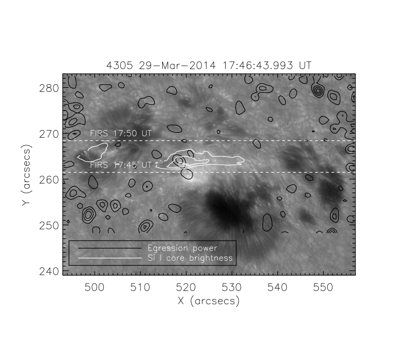
Figure 1: A G-band image centered near 430.5 nm from the Dunn Solar Telescope is shown along with two sets of contours. The black contours are of egression power, $|H_{+}(r,t)|^{2}$, referred to in the text. The white contours are of core intensity of the 1082.7 nm line of Si I. The FIRS data were acquired between 17:40:12 and 18:01:39 UT by stepping the slit (horizontal in the figure) in the Y-direction (S-N). The positions of the slit during the flare are shown as dashed lines. The absolute heliographic coordinates of our ground-based data are accurate to 1 second of arc, as obtained by co-alignment with a continuum image from HMI obtained at 17:50:00 UT.

Figure 6: The results of nLTE calculations are shown. The atmospheric structure is shown in the left panels, emergent intensities are shown in the right panels, for a heliocentric angle with cosine of 0.95. Two “flare models” are shown, exploring the depths and magnitudes of enhanced temperatures in the flaring atmosphere. Typical observed profiles of the flare ribbon and a non-flaring region from the same exposure are shown as thin solid and dotted lines respectively. The upper panels show a “deep penetration” model. The lower panels allow penetration to a depth near 600 km such that the Si I line is in emission, but is a shallow penetration model. Notice that the shallow model predicts no detectable increase in continuum emission and it produces a line emission core that is in qualitative disagreement with the data.

References

- Abbett and Hawley (1999) Abbett, W. P. and Hawley, S. L.: 1999, Astrophys. J. 521, 906
- Allen (1973) Allen, C. W.: 1973, Astrophysical Quantities, Athlone Press, Univ. London
- Allred et al. (2005) Allred, J. C., Hawley, S. L., Abbett, W. P., and Carlsson, M.: 2005, Astrophys. J. 630, 573
- Asensio Ramos et al. (2008) Asensio Ramos, A., Trujillo Bueno, J., and Landi Degl’Innocenti, E.: 2008, Astrophys. J. 683, 542
- Ayres (1979) Ayres, T. R.: 1979, Astrophys. J. 228, 509
- Carmichael (1964) Carmichael, H.: 1964, NASA Special Publication 50, 451
- Casini et al. (2012) Casini, R., de Wijn, A. G., and Judge, P. G.: 2012, ApJ 757, 45
- De Rosa et al. (2009) De Rosa, M. L., Schrijver, C. J., Barnes, G., Leka, K. D., Lites, B. W., Aschwanden, M. J., Amari, T., Canou, A., McTiernan, J. M., Régnier, S., Thalmann, J. K., Valori, G., Wheatland, M. S., Wiegelmann, T., Cheung, M. C. M., Conlon, P. A., Fuhrmann, M., Inhester, B., and Tadesse, T.: 2009, Astrophys. J. 696, 1780
- Donea (2011) Donea, A.: 2011, Space Sci. Rev. 158, 451
- Donea and others (2014) Donea, A. and others, . .: 2014, in preparation
- Donea et al. (1999) Donea, A.-C., Braun, D. C., and Lindsey, C.: 1999, 513, L143
- Donea and Lindsey (2005) Donea, A.-C. and Lindsey, C.: 2005, Astrophys. J. 630, 1168
- Fletcher et al. (2011) Fletcher, L., Dennis, B. R., Hudson, H. S., Krucker, S., Phillips, K., Veronig, A., Battaglia, M., Bone, L., Caspi, A., Chen, Q., Gallagher, P., Grigis, P. T., Ji, H., Liu, W., Milligan, R. O., and Temmer, M.: 2011, Space Sci. Rev. 159, 19
- Fletcher et al. (2007) Fletcher, L., Hannah, I. G., Hudson, H. S., and Metcalf, T. R.: 2007, Astrophys. J. 656, 1187
- Fosbury (1973) Fosbury, R. A. E.: 1973, A&A 27, 129
- Gilbert et al. (2002) Gilbert, H. R., Hansteen, V. H., and Holzer, T. E.: 2002, Astrophys. J. 577, 464
- Hirayama (1974) Hirayama, T.: 1974, Sol. Phys. 34, 323
- Jaeggli (2011) Jaeggli, S.: 2011, Ph.D. thesis, University of Hawaii
- Jefferies et al. (1989) Jefferies, J., Lites, B., and Skumanich, A.: 1989, Astrophys. J. 343, 920
- Judge (2007) Judge, P.: 2007, THE HAO SPECTRAL DIAGNOSTIC PACKAGE FOR EMITTED RADIATION (haos-diper) Reference Guide (Version 1.0), Technical Report NCAR/TN-473-STR, National Center for Atmospheric Research
- Judge (2010) Judge, P. G.: 2010, Mem. Soc. Astron. Italiana 81, 543
- Judge et al. (2004) Judge, P. G., Elmore, D. F., Lites, B. W., Keller, C. U., and Rimmele, T.: 2004, Applied Optics: optical technology and medical optics 43, issue 19, 3817
- Kerr and Fletcher (2014) Kerr, G. S. and Fletcher, L.: 2014, Astrophys. J. 783, 98
- Kopp and Pneuman (1976) Kopp, R. and Pneuman, G.: 1976, Sol. Phys. 50, 85
- Kosovichev (2014) Kosovichev, A. G.: 2014, in J. A. Guzik, W. J. Chaplin, G. Handler, and A. Pigulski (Eds.), IAU Symposium, Vol. 301 of IAU Symposium, p. 349
- Kosovichev and Zharkova (1999) Kosovichev, A. G. and Zharkova, V. V.: 1999, Sol. Phys. 190, 459
- Lagg et al. (2004) Lagg, A., Woch, J., Krupp, N., and Solanki, S. K.: 2004, Astron. Astrophys. 414, 1109
- Lindsey and Braun (2000) Lindsey, C. and Braun, D. C.: 2000, 192, 261
- Linsky and Avrett (1970) Linsky, J. L. and Avrett, E. H.: 1970, Publ. Astron. Soc. Pac. 82, 169
- Lites (1987) Lites, B. W.: 1987, Applied Optics 26, 3838
- Lites et al. (2008) Lites, B. W., Kubo, M., Socas-Navarro, H., Berger, T., Frank, Z., Shine, R., Tarbell, T., Title, A., Ichmoto, K., Katsukawa, Y., Tsuneta, S., Sumematsu, Y., Shimizu, T., and Nagata, S.: 2008, Astrophys. J. 672, 1237
- López Ariste and Casini (2002) López Ariste, A. and Casini, R.: 2002, Astrophys. J. 575, 529
- Machado et al. (1989) Machado, M. E., Emslie, A. G., and Avrett, E. H.: 1989, Sol. Phys. 124, 303
- Martínez-Oliveros et al. (2008) Martínez-Oliveros, J. C., Donea, A.-C., Cally, P. S., and Moradi, H.: 2008, Mon. Not. R. Astron. Soc. 389, 1905
- Martínez Oliveros et al. (2012) Martínez Oliveros, J.-C., Hudson, H. S., Hurford, G. J., Krucker, S., Lin, R. P., Lindsey, C., Couvidat, S., Schou, J., and Thompson, W. T.: 2012, Astrophys. J. Lett. 753, L26
- Murray et al. (2012) Murray, S. A., Bloomfield, D. S., and Gallagher, P. T.: 2012, Sol. Phys. 277, 45
- Sánchez Cuberes et al. (2000) Sánchez Cuberes, M., Bonet, J. A., Vázquez, M., and Wittmann, A. D.: 2000, Astrophys. J. 538, 940
- Schou et al. (2012) Schou, J., Scherrer, P. H., Bush, R. I., Wachter, R., Couvidat, S., Rabello-Soares, M. C., Bogart, R. S., Hoeksema, J. T., Liu, Y., Duvall, T. L., Akin, D. J., Allard, B. A., Miles, J. W., Rairden, R., Shine, R. A., Tarbell, T. D., Title, A. M., Wolfson, C. J., Elmore, D. F., Norton, A. A., and Tomczyk, S.: 2012, 275, 229
- Seaton (1962) Seaton, M. J.: 1962, Proc. Phys. Soc. 79, 1105
- Seaton (1987) Seaton, M. J.: 1987, J. Phys. B: At. Mol. Phys. 20, 6363
- Socas-Navarro (2003) Socas-Navarro, H.: 2003, Melanie. Milne-Eddington Line Analaysis using a Numerical Inversion Engine, Technical report, HAO, NCAR
- Socas-Navarro (2005a) Socas-Navarro, H.: 2005a, Astrophys. J. Lett. 633, L57
- Socas-Navarro (2005b) Socas-Navarro, H.: 2005b, Astrophys. J. Lett. 631, L167
- Spiegel (1957) Spiegel, E. A.: 1957, Astrophys. J. 126, 202
- Sturrock (1966) Sturrock, P. A.: 1966, Nature 211, 695
- Sudol and Harvey (2005) Sudol, J. J. and Harvey, J. W.: 2005, ApJ 635, 647
- Uitenbroek (2000) Uitenbroek, H.: 2000, Astrophys. J. 531, 571
- Uitenbroek (2011) Uitenbroek, H.: 2011, in J. R. Kuhn, D. M. Harrington, H. Lin, S. V. Berdyugina, J. Trujillo-Bueno, S. L. Keil, and T. Rimmele (Eds.), Solar Polarization 6, Vol. 437 of Astronomical Society of the Pacific Conference Series, 439
- Vernazza et al. (1973) Vernazza, J., Avrett, E., and Loeser, R.: 1973, Astrophys. J. 184, 605
- Vernazza et al. (1976) Vernazza, J., Avrett, E., and Loeser, R.: 1976, Astrophys. J. Suppl. Ser. 30, 1
- Vernazza et al. (1981) Vernazza, J., Avrett, E., and Loeser, R.: 1981, Astrophys. J. Suppl. Ser. 45, 635
- Wang (1992) Wang, H.: 1992, Sol. Phys. 140, 85
- Wang et al. (2012a) Wang, H., Deng, N., and Liu, C.: 2012a, Astrophys. J. 748, 76
- Wang et al. (2012b) Wang, S., Liu, C., Liu, R., Deng, N., Liu, Y., and Wang, H.: 2012b, Astrophys. J. Lett. 745, L17