Abstract. We examine the motions of particles in quadrupole ion traps as a function of damping and trapping forces, including cases where nonlinear damping or nonlinearities in the electric field geometry play significant roles. In the absence of nonlinearities, particles are either damped to the trap center or ejected, while their addition brings about a rich spectrum of stable closed particle trajectories. In three-dimensional (3D) quadrupole traps, the extended orbits are typically confined to the trap axis, and for this case we present a 1D analysis of the relevant equation of motion. We follow this with an analysis of 2D quadrupole traps that frequently show diamond-shaped closed orbits. For both the 1D and 2D cases we present experimental observations of the calculated trajectories in microparticle ion traps. We also report the discovery of a new collective behavior in damped 2D microparticle ion traps, where particles spontaneously assemble into a remarkable knot of overlapping, corotating diamond orbits, self-stabilized by air currents arising from the particle motion.

1 Introduction

Electrodynamic ion traps, also known as Paul traps or quadrupole ion traps (QITs), have found a broad range of applications in physics and chemistry, including precision mass spectrometry [1], quantum computing [2], and improved atomic frequency standards [3]. When trapping atomic or molecular ions, QITs often operate with radiofrequency electric fields in vacuum, and the particle dynamics in these traps have been well studied over many decades [1, 4, 5].

Microparticle quadrupole ion traps (MQITs) are also commonly used to measure the detailed properties of individual charged particles in the 100 nm to 100 $\mu$m size range, including aerosols [6, 7], liquid droplets [8, 9], solid particles [10, 11, 12], nanoparticles [13, 14], and even microorganisms [15, 16]. MQITs have also become popular in physics teaching, as they provide a fascinating and somewhat counterintuitive demonstration of oscillatory mechanics and electric forces. Moreover, MQITs are quite inexpensive to construct, levitating particles in air using 50-60 Hz electric fields, making them well suited for teaching [17, 18, 10]. Besides individual particles, MQITs can also trap large numbers of charged particles that self-organize into Coulomb crystalline structures [18, 10, 19].

The addition of motional damping, for example from gas damping or laser cooling, significantly alters the particle dynamics in QITs, and there has been considerable interest in understanding these effects [20, 21, 22, 23, 25], particularly in spectroscopic applications when weak damping is used to stabilize the particle motions [5]. For the simplest and best-studied case – linear damping in purely quadrupolar electric fields – the addition of damping enlarges and shifts the stability regions in parameter space [21], but the boundaries between stable and unstable regions remain sharp. In other words, particles either spiral down until they are at rest at the trap center, or the oscillating electric forces overpower the damping and eject particles from the trap. Thus for the simplest damped QITs, the only stable dynamical solution to the trap equations is the $\vec{x}(t)=0$ solution.

We have found, however, that the situation changes markedly with the addition of weak nonlinearities in the trap equations – either nonlinearities in the field geometry (a deviation from a pure quadrupole field configuration) or nonlinearities in the damping. In both cases the boundaries between stable and unstable regions in parameter space may no longer be sharp, and nontrivial stable solutions to the trap equations appear. We use the term “extended orbits” for these solutions, describing particles that execute stable, closed oscillatory trajectories within a damped ion trap.

We have calculated and experimentally confirmed several examples of these extended orbits, as described below. Nonlinear field geometries in QITs have been investigated by several authors [24, 26, 27, 28, 29], but to our knowledge the different types of extended orbits in damped nonlinear QITs have not previously been characterized. We have found that these states appear quite readily in MQITs when the drive voltage is sufficiently high. After observing this behavior frequently in our own laboratory investigations, we also identified similar examples in online videos [30, 31]. Although it appears that extended orbital behaviors are fairly common in MQITs, we were not able to find an adequate explanation of these observations in our literature search.

The detailed characteristics of an extended orbit depends on the trapped particle properties, including its charge, mass, and radius, so the appearance of a specific dynamical behavior could serve as a convenient and accurate measurement tool in MQITs. And since the extended orbits are stable, measurements of the orbital properties are nondestructive in that they do not eject particles from the trap. Although we have identified several examples of extended orbital behavior, the parameter space of nonlinearities in trap geometry is large, so additional examples may exist. Whether any of these novel dynamical behaviors can be gainfully harnessed in ion trapping applications remains a question for additional study.

2 Axial Motion in 3D Damped Ion Traps

To connect to the existing ion-trapping literature, we begin with a description of the equations of motion for a single charged particle in a purely quadrupolar field geometry with the simplest linear damping, following the standard notation [20, 5]. In particular, we consider a 3D quadrupole trap in cylindrical $(r,z)$ coordinates [5], focusing on the equation of motion describing the axial motion $z(t).$ In our damped 3D MQITs, the extended orbits we have observed were all confined to the $z$ axis. The radial trapping forces, including damping, keep the particle confined to $r=0$ even in the presence of extended motions in $z$, reducing the dynamical problem to one dimension. Although the 1D equation of motion cannot fully describe all aspects of particle motion in a 3D damped ion trap [21], we have nevertheless found that it captures the essence of the extended orbits we have observed. We therefore begin with the the simpler 1D problem as a means of characterizing these extended orbital motions.

We write the particle equation of motion

$$m\frac{d^{2}z}{dt^{2}}+\gamma\frac{dz}{dt}=QE_{z}(z,t)$$ (1)

where $z$ is axial position in the trap, $m$ is particle mass, $\gamma$ is the linear damping coefficient, $Q$ is the particle charge, and $E_{z}$ is the axial electric field. Including AC and DC quadrupole electric fields then gives the standard trap equation

$$\frac{d^{2}z}{d\xi^{2}}+b\frac{dz}{d\xi}+\left[a-2q\cos\left(2\xi\right)\right]z=0$$ (2)

where $\xi=\Omega t/2$ is the dimensionless time, $b=2\gamma/m\Omega$ is the damping parameter, $a=-4QA_{DC}/m\Omega^{2}$ is the DC electric force parameter, $E_{DC}=A_{DC}z$ is the DC electric field, $q=2QA_{AC}/m\Omega^{2}$ is the AC force parameter, and $E_{AC}=A_{AC}z\cos\left(2\xi\right)$ is the AC electric field.

Previous treatments of damped QITs in the absence of nonlinearities (in either the damping or the electric field geometry) [20, 21, 22, 23] have shown that it is possible to eliminate the $dz/d\xi$ term by substituting $z=u\exp\left(-b\xi/2\right),$ giving

$$\frac{d^{2}u}{d\xi^{2}}+\left[\tilde{a}-2q\cos\left(2\xi\right)\right]u=0$$ (3)

where $\tilde{a}=a-b^{2}/4.$ This equation has the form of the Mathieu equation, which has a well-studied stability diagram [5, 4]. As is described in [20, 21], stability in $z$ is different from stability in $u,$ owing to the additional $\exp\left(-b\xi/2\right)$ factor. In [21] the authors plot stability diagrams in the $(a,q)$ plane for several nonzero $b$ values, showing that the stable regions are larger and shifted relative to the corresponding regions when $b=0.$ As described in these references, particles decay to $z=0$ within the stable regions of parameter space, and are expelled from the trap outside the stable regions.

In our experiments with MQITs, the particles are large enough that the gravitational force is significant, plus we often add a uniform electric field $E_{0}$ that produces a constant force similar to gravity. With both forces in the $z$ direction, this adds an additional downward force $mg_{eff}=(mg+QE_{0})$ to Equation 1. After transformations and focusing on the $a=0$ special case, Equation 2 becomes

$$\frac{d^{2}\tilde{z}}{d\xi^{2}}+b\frac{d\tilde{z}}{d\xi}-2q\tilde{z}\cos\left(2\xi\right)=-1$$ (4)

where $\tilde{z}=z\Omega^{2}/4g_{eff},$ and the other parameters are the same as above.

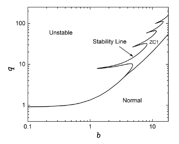
Figure 1: Stability diagram in $(b,q)$ describing solutions to Equation 4. Above the labeled stability line, particles are ejected from the trap. Below the stability line, in the “Normal” region, particles exhibit a simple oscillatory behavior with $\tilde{z}<0$ for all $\xi.$ In the ZC1 region, particles exhibit extended zero-crossing orbits. Examples of both these behaviors are shown in Figure 2.

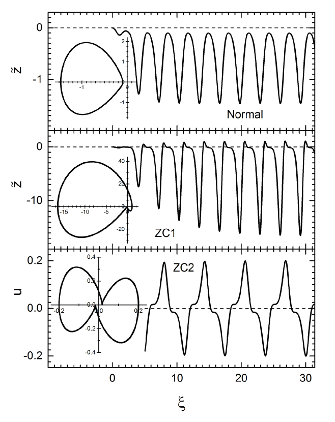
Figure 2: Examples of the Normal (top), ZC1 (middle), and ZC2 (bottom) extended orbits. The top two panels show $\tilde{z}(\xi)$ from solving Equation 4 (assuming a nonzero $g_{eff})$ starting with the initial conditions $\tilde{z}(0)=d\tilde{z}/d\xi(0)=0.$ These two solutions show the particle dropping down to a stable periodic orbit after a few oscillation periods. The bottom panel shows $u(\xi)$ from solving Equation 5 (which assumes $g_{eff}=0)$ after a stable orbit has been achieved. Note that the period of the ZC2 orbit is twice that of the ZC1 orbit. The insets in all three panels show Poincaré plots of $d\tilde{z}/d\xi$ versus $\tilde{z}$ (or $du/d\xi$ versus $u)$ after each particle has reached a stable orbit. These three examples are intended only to show the essential morphologies of the most common Normal, ZC1, and ZC2 extended orbits; the orbital amplitudes and other details depend on the specific parameters used in the equations.

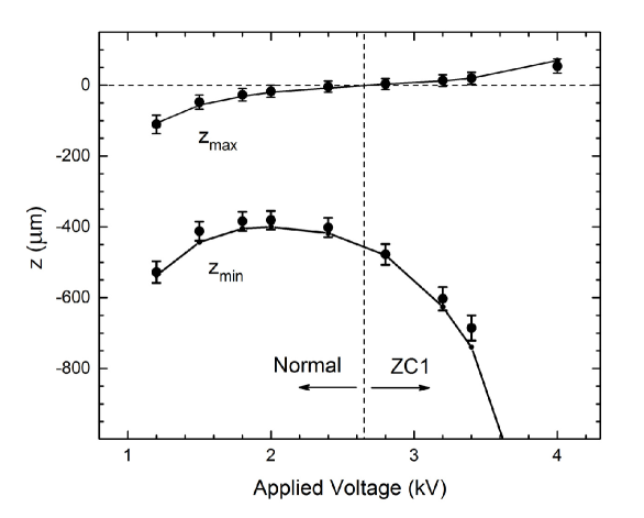
Figure 3: A comparison of measured $z_{\min}$ and $z_{\max}$ for a particle in a MQIT (points) with model calculations (lines). The particle behavior transitioned from Normal on the left to a ZC1 zero-crossing orbit on the right.

With the additional constant force, there is an accompanying change in the particle dynamics, which we investigated by integrating Equation 4 to directly observe the dynamical behavior of $\tilde{z}(\xi)$ for input $b,$ $q,$ and the initial conditions $\tilde{z}$ and $d\tilde{z}/d\xi$ at $\xi=0.$ For this we used NDSolve in Mathematica, which could typically compute 20-30 orbital periods before encountering numerical instabilities. This was usually sufficient for our purposes, as the solutions $\tilde{z}(\xi)$ usually settled quickly into stable orbits that were insensitive to the chosen initial conditions. In difficult cases, we performed longer integrations using ode45 in Matlab. By examining computed particle trajectories with many different inputs, we obtained the results shown in Figure 1.

When $q$ is above the stability line shown in Figure 1, the solutions are unbounded and particles are ejected from the trap. Below the stability line, in the Normal region shown in the figure, the gravitational force pulls particles down to $\tilde{z}<0,$ where they exhibit simple oscillatory micromotion. These orbits are stable, as the average trapping force balances gravity, and an example of this simple motion is shown in the top panel in Figure 2.

In the ZC1 region in Figure 1, particles exhibit zero-crossing orbits (i.e. the motion passes through $\tilde{z}=0$), and again an example is shown in the middle panel of Figure 2. From Figure 1 we see that the ZC1 orbits only occur for $b>3.5,$ when the particle motion is sufficiently overdamped. In the Normal region, increasing $q$ pulls the particle closer to the trap center at $\tilde{z}=0.$ In the ZC1 region, however, increasing $q$ results in an orbit with a greater overall extent, which grows to infinity as the stability line is approached.

Since $\tilde{z}=z\Omega^{2}/4g_{eff},$ we see that $z\rightarrow 0$ as $g_{eff}\rightarrow 0,$ and for $g_{eff}=0$ we confirmed in our numerical analysis that the stability line in Figure 1 separates stable solutions that decay to $z=0$ from unstable solutions that eject particles from the trap, This is consistent with the fact that Equation 4 reduces to the Mathieu equation for $g_{eff}=0$, and the stability line in Figure 1 is consistent with the related analysis presented in [21].

We confirmed the calculated behavior using a MQIT operating at $\Omega/2\pi=60$ Hz, loaded with a single Borosilicate glass microsphere having a specified density of 2230 kg/m³. A microscope objective built into the MQIT allowed us to image the trapped particle directly, yielding a measured diameter of $2R=9\pm 2$ $\mu$m, which was consistent with the nominal diameter of $10\pm 1$ $\mu$m specified by the manufacturer. Balancing gravity with a constant electric field $E_{0}$ gave a measured $Q/m=g/E_{0}=0.0176\pm 0.0015$ C/kg. Using Stoke’s-law damping in air ($\gamma=6\pi\mu R,$ with $\mu=1.8\times 10^{-5}$ kg/m-s) gave $b=9.5\pm 3,$ and the electric field $E_{z}(z,t)$ was calculated from the known geometry of the trap, giving $q$ as a function of the applied voltage.

With all the relevant particle and trap properties determined, we were able to create a model of the particle behavior with no free parameters for comparison with experiment. The uncertainty in the particle radius was rather large, however, so in the end we adjusted this parameter (within the stated uncertainty limits) to better fit the data, thus essentially using the orbital motion to measure $R$. We measured and calculated $z_{\min}$ and $z_{\max}$, the extrema of the particle motion (which was purely axial) as a function of the applied voltage. Figure 3 shows results with no bias field to counteract gravity $(E_{0}=0).$ The smooth transition from Normal to ZC1 behavior was essentially as calculated, and we also confirmed (not shown in the figure) that the overall scale of the motion was proportional to $g_{eff}.$

From this and other observations of orbital behaviors in MQITs, we confirmed the simple 1D theory for a 3D quadrupole trap with linear damping and the addition of a constant gravity-like force. The Normal and ZC1 orbits were observed as purely axial motions, and our measurements showed good quantitative agreement with calculations.

2.1 Nonlinear Damping

In MQITs, the Reynolds number of the motion is often of order unity or higher, requiring an additional damping force proportional to $v^{2}=(dz/dt)^{2},$ giving the total damping force $-\gamma v\left(1+\alpha\left|v\right|\right),$ where $\gamma$ describes the linear damping and $\alpha$ is a nonlinear damping constant [32]. For the zero-gravity case with no DC fields $(a=0),$ the equation of motion then becomes

$$\frac{d^{2}u}{d\xi^{2}}+b\frac{du}{d\xi}\left[1+\left|\frac{du}{d\xi}\right|\right]-2qu\cos\left(2\xi\right)=0$$ (5)

where $u=\alpha\Omega z/2.$ A dynamical analysis of the solutions to this equation yields the stability diagram shown in Figure 4.

As this is a zero-gravity case, the solutions below the stability line are all damped to $u=0.$ This makes physical sense, since the additional nonlinear damping can only increase the stability. Above the stability line, however, the increased damping is sufficient to prevent the realization of any unbounded solutions that eject particles from the trap. Just above the lowest branch of the stability line, particles exhibit a new type of stable zero-crossing orbit we label ZC2, and an example of this motion is shown in the third panel in Figure 2. Since the particle spends one AC cycle above $u=0$ and one AC cycle below, the total period is $4\pi/\Omega,$ double the period of the AC drive and the other orbital motions described above, as shown in Figure 2.

For higher $b,$ again just above the stability line, particles exhibit stable ZC1 or ZC2 orbits as shown in Figure 4. Note that the ZC1 orbits arising from the nonlinear Equation 5 occur for $g_{eff}=0,$ although their morphology is essentially the same as we found with the linear $g_{eff}\neq 0$ case described above. Since there is no effective gravity to break the up/down symmetry in Equation 5, a ZC1 orbit may point up or down depending on initial conditions. Note also that the boundaries between the ZC1 and ZC2 regions are not sharp, especially at high $q,$ where the particle motions are sensitive to initial conditions and may be aperiodic. The ZC1 and ZC2 regions are quite distinct just above the stability line, however, segregating the two morphologies as shown in Figure 4.

The physical size of an extended particle orbit depends on the nonlinear damping via $z=2u/\alpha\Omega,$ so as expected $z$ becomes unbounded above the stability line as $\alpha\rightarrow 0.$ This makes it possible to measure the nonlinear damping coefficient directly at low Reynolds number by observing the ZC2 orbital behavior in a MQIT, perhaps to higher accuracy than has been accomplished to date by more traditional means [32]. For example, for $b<2$ the physical size of a ZC2 orbit scales approximately as $z\sim 1/\gamma\alpha.$ The linear damping coefficient is typically Stoke’s damping in a MQIT, so the nonlinear damping coefficient $\alpha$ can be extracted from a measurement of the orbital size.

In our MQITs we have found that the ZC2 orbital behavior is quite common, and Figure 5 shows one example. To obtain this measurement we strobed the laser illuminating the particle near 30 Hz, allowing the particle position to be measured from a simple video recording of the motion. Again the overall characteristics of the observed motion are well described by the 1D equation of motion. Another example showing ZC2 axial motion can be found in [30].

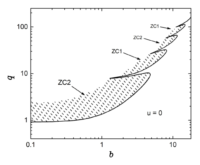
Figure 4: A stability diagram for the zero-gravity case with $a=0$ and an additional nonlinear damping term, described by Equation 5. The stability line is identical to that shown in Figure 1. Below the stability line, all solutions decay to $u=0.$ Above the stability line, the nonlinear damping causes all solutions to be bounded, so no particles are ejected from the trap. Just above the stability line, particles exhibit stable ZC1 or ZC2 orbital behaviors that are largely independent of initial conditions, as labeled in the diagram. Far above the stability line, the particle behavior is typically aperiodic and strongly dependent on initial conditions.

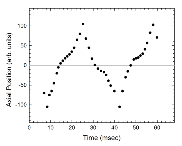
Figure 5: Measurements of a typical ZC2 orbit in a 60 Hz MQIT, showing the axial motion $z(t).$ The radial motion was confined to $r=0$ in the trap. The zero point of the measured motion presented in the plot is relative to the trap center, as determined by cancelling gravity and observing the stable position of the particle at $z=0.$ The overall characteristics of the orbital motion are consistent with that shown in Figure 2, including the 30 Hz oscillation frequency.

2.2 Nonlinear Electric Fields

We have also examined particle behavior when the electric field geometry deviates from the linear $E_{AC}(z)=A_{AC}z$ found in a pure quadrupole ion trap. There are many simple MQIT geometries in which the electric field rolls off at high $z,$ and we model these nonlinear field geometries using $E_{AC}(z)=k^{-1}A_{AC}\tan^{-1}(kz),$ where $k$ sets the scale of the rolloff in the field. With this functional form the field is approximately linear when $z\ll k^{-1},$ reaching a constant value when $z\gg k^{-1},$ and taking $k\rightarrow 0$ returns the purely linear field. With this change, the equation of motion becomes

$$\frac{d^{2}\tilde{u}}{d\xi^{2}}+b\frac{d\tilde{u}}{d\xi}-2q\tan^{-1}(\tilde{u})\cos\left(2\xi\right)=0$$ (6)

for the case $a=0$ and $g_{eff}=0,$ where $\tilde{u}=kz.$ Analyzing this yields a stability diagram quite similar to that shown in Figure 4, featuring both ZC1 and ZC2 extended orbits. Again the orbits decay to $\tilde{u}=0$ below the stability line, and there are no unbounded solutions above this line. Examining other electric field configurations (for example $E=Ak^{-1}\log(1+kz)$ and $E=Az/(k^{3}z^{3}+1)$), we found that the stability diagrams were all similar to that shown in Figure 4, as long as the field rolled off at high $z.$

In [25] the authors describe calculated axial ZC2 orbits in a 3D QIT with linear damping in a purely quadrupole field geometry, in contradiction to our results. We also found, however, that a ZC2-like behavior could be seen in the absence of nonlinearities when sufficiently close to the stability line, and this may explain the discrepancy with [25]. Integrating the equation of motion for $\sim 20$ orbital periods (using Mathematica) can yield a ZC2-like orbit that appears to be stable, but integrating with the same parameters for several hundred periods (using Matlab) reveals that these orbits are in fact slowly decaying. We only found truly stable extended orbits with the addition of nonlinear damping or nonlinear field geometries, or both.

3 2D Damped Ion Traps

For the case of a two-dimensional quadrupole field with a nonlinear damping force $\vec{F}_{damping}=-\gamma\vec{v}\left(1+\alpha\left|\vec{v}\right|\right)$, the equations of motion in $(x,y)$ coordinates can be rescaled to become

$$\frac{d^{2}\hat{x}}{d\xi^{2}}+b\frac{d\hat{x}}{d\xi}\left[1+\left|\hat{v}\right|\right]-2q\hat{x}\cos\left(2\xi\right) = 0$$ (7)

$$\frac{d^{2}\hat{y}}{d\xi^{2}}+b\frac{d\hat{y}}{d\xi}\left[1+\left|\hat{v}\right|\right]+2q\hat{y}\cos\left(2\xi\right) = 0$$

where $\hat{x}=\alpha\Omega x/2,$ $\hat{y}=\alpha\Omega y/2,$ $b=2\gamma/m\Omega$, $q=2QA/m\Omega^{2}$, the AC electric field is $\left(E_{x},E_{y}\right)=\left(Ax,-Ay\right),$ and $\left|\hat{v}\right|=\alpha\left|\vec{v}\right|=[\left(d\hat{x}/d\xi\right)^{2}+\left(d\hat{y}/d\xi\right)^{2}]^{1/2}.$ Here we have assumed zero DC electric field and $g_{eff}=0.$ In the absence of nonlinear damping $(\alpha=0),$ these equations decouple to the 1D case above, yielding the same stability line shown in Figure 1. Since we are taking $g_{eff}=0$ in this case, our numerical analysis confirmed that particles either decay to $(x,y)=0$ below the stability line or are ejected from the trap above the stability line.

Including nonlinear damping, however, yields a rich spectrum of stable extended orbits, as shown in Figure 6. The diamond-shaped orbits are rounded for $b<2$ and develop cusp-like corners at higher $b.$ The orbits are typically more asymmetrical (as shown in the uppermost example of the three diamond plots) at higher $b$ and higher $q$, where the symmetry is more sensitive to initial conditions. Above the second branch of the stability line, particles are driven into “bowtie” orbits, while more complex “cloverleaf” orbits appear above the third branch, as indicated in the figure. These orbits are most stable when $q$ is just above the stability line, while at high $q$ the motion can be aperiodic and strongly dependent on initial conditions.

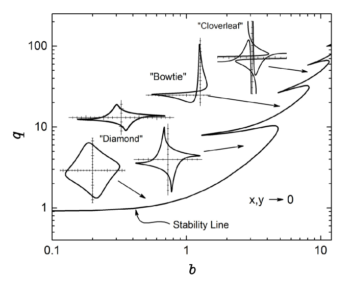
Figure 6: The stability diagram for a 2D quadrupole trap with nonlinear damping, describing solutions to Equation 7. Below the stability line, particles are damped to the center of the trap at $(x,y)=0.$ Above the stability line, in roughly the same regions shown in Figure 4, particles are driven into a variety of stable extended orbits as shown. The inset plots show examples of calculated closed particle orbits in $(x,y)$ space; the cloverleaf plot shows only the inner region of the orbit. As with Figure 2, the inset diagrams here are intended only to show the morphologies of the different types of extended orbits; the orbital amplitudes and other details depend on the specific parameters used in the equations.

Note there are many similarities between the 1D and 2D orbits occurring in 3D and 2D quadrupole traps, respectively. For example, a diamond orbit is essentially a ZC2 orbit in both $x$ and $y,$ while a bowtie orbit is like a ZC1 orbit in both $x$ and $y.$ The 2D orbits correspond to their 1D analogs in the stability diagram as well, as can be seen by comparing Figure 6 and Figure 4. Similarly, the orbital period is $2\pi/\Omega$ for the bowties and ZC1 orbits, while it is $4\pi/\Omega$ for the diamonds, cloverleafs, and ZC2 orbits.

Experimentally the diamond orbits are the easiest to obtain, as they require low damping and a corresponding low drive voltage. The other orbits occur for larger $b$, and a much larger $q$ is therefore needed to get above the stability line. To date we have only observed diamond and bowtie orbits in our 2D MQITs, and Figure 7 shows two examples. Diamond orbits can also be seen in the online videos [30, 31], suggesting that they are somewhat common in MQITs. We have observed symmetrical and asymmetrical diamond orbits, along with a variety of odd time-dependent behaviors we do not yet understand. Diamond orbits with slowly oscillating changes in the orbital asymmetry were especially common at low $b$, and this behavior remains puzzling. Some of these behaviors may be driven by residual air currents within the traps.

The images in Figure 7 were obtained in a “4-bar” MQIT consisting of four identical conducting bars, collinear in the $z$ direction and arranged on the corners of a square in the $xy$ plane [19]. The bars had a diameter of 3.2 mm, and their nearest separation was 6.7 mm. An AC voltage was applied to the bars with alternating polarities to produce approximately quadrupolar electric fields in $x$ and $y,$ with no electric forces in the $z$ direction. The trap operated at 60 Hz in air, with applied voltages up to 6 kV. Although the electric field geometry in a 4-bar trap is not a pure quadrupole field, our calculations showed that no extended orbits were possible in a 4-bar trap in the absence of nonlinear damping. Thus the behavior of a 4-bar trap is qualitatively the same as a 2D quadrupole trap.

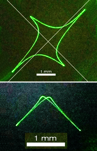
Figure 7: Examples of a diamond (top) and bowtie (bottom) orbit observed in a 4-bar MQIT with $g_{eff}=0$. The two photographs show single particles executing stable closed orbits in the $xy$ plane, illuminated by a laser. The exposure times were longer than the orbital periods, causing the particles to appear as streaks delineating the orbital paths. Diagonal lines were digital superimposed on the top image to show the axes of the 2D quadrupole, which had the same orientation for both images. Scale bars were also added digitally, and a DC bias electric field canceled the gravitational force.

One especially noteworthy phenomenon we can produce on demand in our 2D MQITs is a collective mode that includes dozens of particles in overlapping corotating diamond orbits. The phenomenon is difficult to describe adequately, and still photos show little more than a blur of rapidly moving trapped particles. Videos are somewhat more informative, and examples can be found at [33]. Based on our observations of the formation, behavior, and decay of this collective mode, we believe it is stabilized by air currents within the trap.

When several particles are initially driven into nearby corotating diamond orbits, we believe that the particle motions create a fan-like effect that pushes air radially outward from the trap; that is, the flow is outward in $x$ and $y$ away from the trap center at $(x,y)=0.$ This radial outflow is accompanied by an axial inflow along the $z$ axis. Since there are no electrical forces in the $z$ direction, the axial inflow pulls the nearby corotating particles together in spite of the repulsive forces arising from their like charges. The result is a frenetic knot of particles moving in overlapping corotating diamond orbits, which we call a “trapnado”.

Once a small trapnado forms, the axial airflow quickly pulls in additional particles that join the knot and reinforce the air motions. Trapnados form easily with either rotation direction, and we have even witnessed axial collisions between two independent trapnados [33], the outcome depending on their relative rotation directions. We discovered trapnados serendipitously in our 4-bar MQITs, and we believe that our hypothesis of air-stabilized diamond orbits provides a sound (albeit qualitative) physical explanation for this remarkable phenomenon.

4 Discussion

Our initial motivation for undertaking this investigation was experimental: we built a number of MQITs operating in air and soon began seeing extended orbital behaviors, both 1D axial orbits in 3D MQITs and diamond-shaped orbits 2D MQITs. Although our online research suggests that others have observed these behaviors numerous times over the past several decades, our literature search did not turn up an adequate characterization or theoretical explanation of the extended orbits.

Our analysis of single-particle trajectories in damped ion traps shows that nonlinearities are required to produce stable extended orbits, in particular either nonlinear damping or nonlinearities in the electric field geometry. In the absence of nonlinearities, particles are either damped to the trap center or ejected from the trap. As has been documented by others, the stability line between damped and ejected is sharp, and the only stable trajectory in this case is the $\vec{x}(t)=0$ solution.

With the addition of nonlinearities, a variety of stable, closed trajectories appear, as described in detail above. We have not examined all possible nonlinearities, as this parameter space is large, so additional novel particle behaviors may exist. Besides 2D quadrupole geometries, we have also calculated diamond-like orbits in 2D hexapole and octapole geometries, where the diamonds then show six or eight corners, respectively. Our focus in the present work was on MQITs operating in air at 60 Hz, driven by experimental considerations, and we have not yet done an additional analysis with a focus on atomic/molecular QITs.

Possible applications include measurements of nonlinearity parameters in ion traps. For example, the orbital motion in a MQIT with nonlinear damping depends strongly on the nonlinearity parameter $\alpha,$ somewhat independently of the linear damping. Because of this, $\alpha$ could be measured directly even when nonlinear damping is a small perturbation of the total damping. In contrast, a measurement of a particle’s terminal velocity (for example) yields the total damping only, so $\alpha$ cannot be extracted independently from such a measurement.

Nonlinearities in the electric field geometry could also be measured using extended orbital motions, and these measurements are nondestructive in that particles are not ejected from the trap. Observing the full range of particle motions both above and below the nominal stability line could allow independent measurements of many particle properties. Tayloring the electric field geometry to facilitate a specific measurement of some kind may be possible.

In addition to calculating single-particle orbits in detail, we also discovered the remarkable trapnado phenomenon described above. We believe this is only the second self-organizing collective behavior seen in MQITs to date, supplementing the well-known Coulomb crystalline structures that have been observed for many decades.

This work was supported in part by the California Institute of Technology and a generous donation by Dr. Richard Karp.

References

- [1] R. E. March and J. F. Todd, “Quadrupole ion trap mass spectroscopy, 2nd edition” Wiley-Interscience (2005).
- [2] H. Haffner, C. F. Roos, and R. Blatt, “Quantum computing with trapped ions,” Phys. Rep. 469, 155-203 (2008).
- [3] D. Leibfried, R. Blatt, C. Monroe, and D. Wineland, “Quantum dynamics of single trapped ions,” Rev. Mod. Phys. 75, 281-324 (2003).
- [4] P. K. Ghosh, “Ion Traps,” Oxford Univ. Press (1996).
- [5] R. E. March, “An introduction to quadrupole ion trap mass spectrometry,” J. Mass Spectrom. 32, 351-369 (1997).
- [6] M. Yang et al., “Real-time chemical analysis of aerosol particles using an ion trap mass spectrometer,” Rapid Comm. Mass Spect. 10, 347-51 (1996).
- [7] D. T. Suess and K. A. Prather, “Mass spectrometry of aerosols,” Chem. Rev. 99, 3007-3036 (1999).
- [8] B. Kramer, O. Hubner, H. Vortisch, et al., “Homogeneous nucleation rates of supercooled water measured in single levitated microdroplets,” J. Chem. Phys. 111, 6521-6527 (1999).
- [9] S. Arnold and L. M. Folan, “Fluorescence spectrometer for a single electrodynamically levitated microparticle,” Rev. Sci. Instrum. 57, 2250–2253 (1986).
- [10] R. F. Wuerker, H. Shelton, and R. V. Langmuir, “Electrodynamic containment of charged particles,” J. Appl. Phys. 30, 342–349 (1959).
- [11] Gina Visan, Ovidiu S. Stoican, “An experimental setup for the study of the particles stored in an electrodynamic linear trap,” Rom. J. Phys. 58, 171-180 (2013).
- [12] S. Schlemmer, J. Illemann, S. Wellert, et al., “Nondestructive high-resolution and absolute mass determination of single charged particles in a three-dimensional quadrupole trap,” J. Appl. Phys. 90, 5410-5418 (2001).
- [13] Y. Cai, W.-P. Peng, S.-J. Kuo et al., “Single-Particle Mass Spectrometry of Polystyrene Microspheres and Diamond Nanocrystals,” Anal. Chem. 74, 232-238 (2002).
- [14] Sung Cheol Seo, Seung Kyun Hong, and Doo Wan Boo, “Single Nanoparticle Ion Trap (SNIT): A Novel Tool for Studying in-situ Dynamics of Single Nanoparticles,” Bull. Korean Chem. Soc. 24, 552-554 (2003).
- [15] W. P. Peng, Y. C. Yang , M. W. Kang, et al., “Measuring masses of single bacterial whole cells with a quadrupole ion trap,” J. Am. Chem. Soc. 126, 11766–11767 (2004).
- [16] Zhiqiang Zhu, Caiqiao Xiong, Gaoping Xu, et al., “Characterization of bioparticles using a miniature cylindrical ion trap mass spectrometer operated at rough vacuum,” Analyst 136, 1305-1309 (2011).
- [17] H. Winter and H. W. Ortjohann, “Simple demonstration of storing macroscopic particles in a ‘Paul trap’,” Am. J. Phys. 59, 807-13 (1991).
- [18] Scott Robertson and Richard Younger, “Coulomb crystals of oil droplets,” Am. J. Phys. 67, 310-315 (1999).
- [19] L. M. Vasilyak, V. I. Vladimirov, L. V. Deputatova, et al., “Coulomb stable structures of charged dust particles in a dynamical trap at atmospheric pressure in air,” New J. Phys. 15, 043047 (2013).
- [20] William B. Whitten, Peter T. A. Reilly, and J. Michael Ramsey, “High-pressure ion trap mass spectroscopy,” Rapid Commun. Mass Spectrom. 18, 1749-1752 (2004).
- [21] Michael Nasse and Christopher Foot, “Influence of background pressure on the stability region of a Paul trap,” Eur. J. Phys. 22, 563-573 (2001).
- [22] N. R. Whetten, “Macroscopic particle motion in quadrupole fields,” J. Vac. Sci. Technol. 11, 515-518 (1974).
- [23] T. Hasegawa and K. Uehara, “Dynamics of a single particle in a Paul trap in the presence of the damping force,” Appl. Phys. B 61, 159-168 (1995).
- [24] I. Ziaeian, S. M. Sadat Kiai, M. Eilahi, et al., “Theoretical study of the effect of ion trap geometry on the dynamic behavior of ions in a Paul trap,” Int. J. Mass Spect. 304, 25-28 (2011).
- [25] Iman Ziaeian and Houshyar Noshad, “Theoretical study of the effect of damping force on higher stability regions in a Paul trap,” Int. J. Mass Spect., 1–5, (2010).
- [26] R. Blumel, “Nonlinear dynamics of trapped ions,” Phys. Scripta A T59, 369-379 (1995).
- [27] I. Garrick-Bethell, T. Clausen, and R. Blumel, R, “Universal instabilities of radio-frequency traps,” Phys Rev. E 69, 056222 (2004).
- [28] Bogdan M. Mihalcea, “Semiclassical dynamics for an ion confined within a nonlinear electromagnetic trap,” Phys. Scripta A T143, 014018 (2011).
- [29] R. Alheit, X. Z. Chu, M. Hoefer, et al., “Nonlinear collective oscillations of an ion cloud in a Paul trap,” Phys. Rev. A 56, 4023-4031 (1997).
- [30] https://www.youtube.com/watch?v=bkYXNeJ8IP0 (posted 2009).
- [31] https://www.youtube.com/watch?v=pqfG-df5ZWk (posted 2012), and related images and videos at http://www.paultrap.jecool.net/en/.
- [32] B. P. Le Clair, A. E. Hamielec, and H. R. Pruppacher, “A numerical study of the drag on a sphere at low and intermediate Reynolds numbers,” J. Atmos. Sci. 27, 308-315 (1970).
- [33] http://newtonianlabs.com/.