Optimal models of extreme volume-prices are time-dependent

Abstract

We present evidence that the best model for empirical volume-price distributions is not always the same and it strongly depends in (i) the region of the volume-price spectrum that one wants to model and (ii) the period in time that is being modelled. To show these two features we analyze stocks of the New York stock market with four different models: $\Gamma$, $\Gamma$-inverse, log-normal, and Weibull distributions. To evaluate the accuracy of each model we use standard relative deviations as well as the Kullback-Leibler distance and introduce an additional distance particularly suited to evaluate how accurate are the models for the distribution tails (large volume-price). Finally we put our findings in perspective and discuss how they can be extended to other situations in finance engineering.

1 Introduction

It has been acknowledge in financial distributions that the statistics of extreme events, leading to heavy tails, as well has correlations between noise sources and other components need to be taken into account if one pretends to establish a model that describe accurately this dynamical system. In this paper we are interested in the study of extreme events present in financial markets distributions. As study subject we shall consider the New York stock market (NYSM). We focus here on the evolution of volume-price, i.e. on changes in capitalization, which should have more the character of a conserved quantity than the price per se. Having access to the overall distribution of volume-price provides information about the entire capital traded in the market. However, extreme events focus in what happens on the right tails of such distributions, the region comprising the highest volume-prices occurring in a given market.

In this paper we will address the problem of modelling such tails at high volume-prices in comparison with models for the full volume-price distribution.

Our data base is composed by $\sim 2000$ listed shares extracted from the NYSM and freely available at http://finance.yahoo.com/. The data has a sample frequency of $0.1$ min^-1, starting in January 27th 2011 and ending in April 6th 2014, with a total of 976 days ($\sim 10^{5}$ data points).

Using this data we build the volume-price distribution of the $\sim 2000$ listed companies every $10$ minutes. We define the volume-price $s=pV$ as the product of the trading volume $V$ and the last trade price $p$. More details, concerning the data mining and collection can be found in Ref. [2].

We start in Sec. 2 by studying the behaviour of volume-price distribution and introducing four different typical models in finance to fit the empirical data[1, 2]. In Sec. 3, we present the error analysis of each models, using standard relative deviations and more sophisticated measures, namely the Kullback-Leibler distance. This measure is particularly suited to evaluate how close the (non-linear) models fit is from the empirical distributions. Section 4 concludes the paper.

2 Four models for volume-price distributions

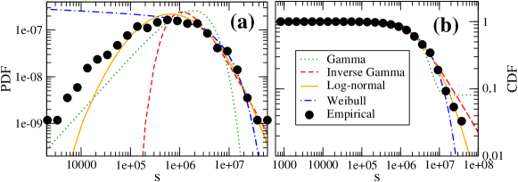
Figure 1: (a) Probability density function and (b) cumulative density function given by the four different distributions: $\Gamma$ (Eq. 1), inverse $\Gamma$ (Eq. 2), log-normal (Eq. 3), and Weibull (Eq. 4).

We will consider four well-known[1] bi-parametric distributions to fit the empirical volume-price distribution, namely the $\Gamma-$distribution:

$$p_{\Gamma}(s)=\frac{s^{\phi-1}}{\theta^{\phi}\Gamma[\phi]}e^{-\frac{s}{\theta}}$$ (1)

the inverse $\Gamma-$distribution:

$$p_{1/\Gamma}(s)=\frac{\theta^{\phi}}{\Gamma[\phi]}s^{-\phi-1}e^{-\frac{\theta}{s}}\$$ (2)

the Log-normal distribution:

$$p_{ln}(s)=\frac{1}{\sqrt{2\pi}\theta s}e^{-\frac{(\log s-\phi)^{2}}{2\theta^{2}}}$$ (3)

the Weibull distribution

$$p_{w}(s)=\frac{\phi}{\theta^{\phi}}s^{\phi-1}e^{-\left(\frac{s}{\theta}\right)^{\phi}\vspace{0.5cm}}$$ (4)

Using the least square scheme, we fit the empirical cumulative density function (CDF) with each one of the four models above. Figures 1a and 1b show respectively the probability and corresponding cumulative density function of each model (lines) that fit the empirical distribution (bullets) at one particular $10$-minute time-step.

While the log-normal and the $\Gamma$-distributions are the best ones for the low range of volume-price values, all four models except $\Gamma$ are closer to the right tail comprising the largest volume-prices observed. Therefore, one should not expect to obtain always the same optimal model, i.e. the smallest deviations or error measures are not observed always for the same model.

In Fig. 2 we show the typical evolution of one parameter during a short time-interval ($\sim 3$ days). Here one plots the parameter $\phi$ of the inverse $\Gamma$-distribution. Similar (qualitative) evolutions are observed with other parameters above.

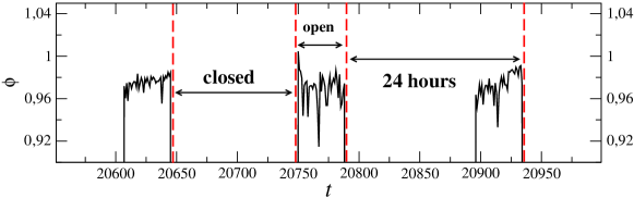
Figure 2: Illustrative time series of the parameter $\phi$ for inverse $\Gamma-$distribution (Eq. 2) during approximately three days. Similar plots are obtain for all parameters in the four models here considered.

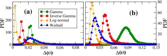
Figure 3: Probability density function of the resulting relative errors (a) $\Delta\phi$ and (b) and $\Delta\theta$, corresponding to the fitting parameters $\phi$ and $\theta$ respectively.

3 What is the best model for our data?

To evaluate how accurate a model is, we first consider the relative error, $\Delta\phi$ and $\Delta\theta$, of each parameter value, $\phi$ and $\theta$ respectively. In Fig. 3a and Fig. 3b one plots the distributions of the observed relative errors.

For both parameters the smallest relative deviation is observed for the log-normal distribution. The inverse $\Gamma$-distribution shows also acceptable deviations. The other two models are not as good as the log-normal and $\Gamma$-distributions. In a previous work, where the evolution of the mean volume-price $\langle s\rangle$ was considered separately and the models were used to fit the distribution of the normalized volume-price, $s/\langle s\rangle$, the optimal model according to relative deviations was only the inverse $\Gamma$-distribution.

The relative deviations do no take into account the importance of the volume-price spectrum in the distribution, weighted by the probability density function or another density function. To weight each value in the volume-price spectrum according to some density function we introduce here the generalized Kullback-Leibler distance:

$$D^{(F)}(P||Q)=\sum_{i}\ln\left(\left\lvert\frac{P(i)}{Q(i)}\right\rvert\right)F(i)\Delta x,$$ (5)

where $Q(i)$ is the empirical distribution, $P(i)$ is the modelled PDF and $F(i)$ is a weighting function. For $F(i)=P(i)$ one obtains the standard Kullback-Leibler distance[3], where the logarithmic deviations are heavier weighted in the central region of the distribution. Figure 4a shows the distribution of the $D^{(P)}$ values obtained when considering each one of the four models. Once again one observes that the log-normal distribution is the one yielding smaller deviations.

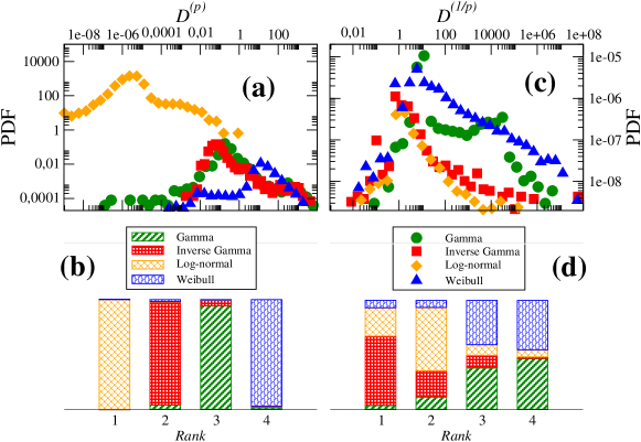
Figure 4: (a) PDF of the Kullback-Leibler distance $D^{(P)}$ test for the full spectrum of the volume-price. (b) Percentage of accuracy rankings for each model, using the Kullback-Leibler distance $D^{(P)}$. A model with rank $1$ is more accurate then a model with rank $2$. (c) PDF of the tail Kullback-Leibler distance $D^{(1/P)}$ (see text) using only the values of $s$ larger the median of the distribution. (d) Percentage of accuracy rankings for each model, using the tail Kullback-Leibler distance $D^{(1/P)}$.

Since the $D^{(P)}$ distributions overlap, one may argue that the log-normal distribution might not be always the best model. To address this question we plot in 4b the ranking ordering all four models in their accuracy for each time step. Indeed, almost always the log-normal is the best model, followed by the inverse $\Gamma$-distribution.

For financial purposes, volume-price values are not equally important. For instance, a deviation from the observed distribution in the region of small volume-prices result in a smaller fluctuation of the amount of transactions than in the region of largest values, where the risk is the highest and therefore should be more accurately fitted.

To weight the largest volume-prices we first consider only the region of the distribution for $s$ larger than the median and then consider in Eq. (5) $F(i)=1/P(i)$. In this way, the largest values of the volume-price, i.e. those for which $P(i)$ is the smallest will be weighted heavier than the others. Figures 4c and 4d show the distance distributions for this case and the corresponding rankings respectively.

Interestingly, not only the best model is the inverse $\Gamma$-distribution but the dominance of one single model in each rank is not strong as when considering the full distributions. This indicates that in NYSM the best model of the volume-price tail distribution is most probably the inverse $\Gamma$-distribution but the probability that another model, most probably the log-normal, is observed as the best one is significative.

4 Conclusions

In this paper we analyzed New York stock market volume-price distributions. By testing four different models, commonly applied in finance, to the empirical volume-price distributions, we found evidence that the best model is not always the same.

In particular, we show that it strongly depends on the region of the spectrum that one wants to model, being the log-normal the best model for low values of $s$ and the inverse $\Gamma$ for the tail distributions. Moreover, the best model seems to change depending on the period of time that the distribution is being modelled.

All in all, our findings put in question common assumptions used when analyzing finance data. Namely, to assume that volume-price distributions are log-normal[4] seems to be valid only under particular restrictions and it seems not to be the optimal model when addressing extreme events. Furthermore, we provided evidence to claim that the non-stationary character of finance data is reflected not only in the fluctuations of the statistical moments defining the empirical distributions of observed values, but also in the functional shape of those distributions.

For further investigation, one can ask what is the reason behind this time dependency. A good study of this strange behaviour can eventually enable one to improve measures of risk and to provide additional insight in risk management.

References

References

- [1] S. Camargo, S.M.D. Queirós and Celia Anteneodo, Eur. Phys. J. B 86 159 (2013).
- [2] P. Rocha, F. Raischel, J. Cruz and P.G. Lind, “Stochastic Evolution of Volume-Price Distributions” submitted in 2014.
- [3] S. Kullback and R.A. Leibler, An. Math. Stat. 22 79–86 (1951).
- [4] M.F.M. Osborne, Operations Research 7 145-173 (1959).