Forbidden oxygen lines at various nucleocentric distances in comets

Abstract

Aims. To study the formation of the [OI] lines - i.e., 5577.339 $\AA$ (the green line), 6300.304 $\AA$ and 6363.776 $\AA$ (the two red lines) - in the coma of comets and to determine the parent species of the oxygen atoms using the green to red-doublet emission intensity ratio, I₅₅₇₇/(I₆₃₀₀+I₆₃₆₄), (hereafter the G/R ratio) and the lines velocity widths.

Methods. We acquired at the ESO Very Large Telescope high-resolution spectroscopic observations of comets C/2002 T7 (LINEAR), 73P-C/Schwassmann-Wachmann 3, 8P/Tuttle, and, 103P/Hartley 2 when they were close to the Earth (¡ 0.6 au). Using the observed spectra, which have a high spatial resolution (¡60 km/pixel), we determined the intensities and the widths of the three [OI] lines. We have spatially extracted the spectra in order to achieve the best possible resolution of about 1-2^′′, i.e., nucleocentric projected distances of 100 to 400 km depending on the geocentric distance of the comet. We have decontaminated the [OI] green line from C₂ lines blends that we have identified.

Results. It is found that the observed G/R ratio on all four comets varies as a function of nucleocentric projected distance (between $\sim$0.25 to $\sim$0.05 within 1000 km). This is mainly due to the collisional quenching of O(¹S) and O(¹D) by water molecules in the inner coma. The observed green emission line width is about 2.5 km s^-1 and decreases as the distance from the nucleus increases which can be explained by the varying contribution of CO₂ to the O(¹S) production in the innermost coma. The photodissociation of CO₂ molecules seems to produce O(¹S) closer to the nucleus while the water molecule forms all the O(¹S) and O(¹D) atoms beyond $10^{3}$ km. Thus we conclude that the main parent species producing O(¹S) and O(¹D) in the inner coma is not always the same. The observations have been interpreted in the framework of the coupled-chemistry-emission model of Bhardwaj & Raghuram (2012) and the upper limits of CO₂ relative abundances are derived from the observed G/R ratios. Measuring the [OI] lines could indeed provide a new way to determine the CO₂ relative abundance in comets.

1 Introduction

Comets are among the best preserved specimens of the primitive solar nebula as the nucleus composition did not evolve much since their formation, 4.6 billion years ago. Studying the composition of comet nuclei is thus essential to understand the formation and the evolution of material within our solar system. Oxygen is one of the most abundant elements in comets since most of the cometary ices are constituted of H₂O, CO₂ and CO molecules. All these molecules coming from the sublimation of cometary ices can produce oxygen atoms in the coma by photodissociation. Oxygen atoms in comets are analyzed through the three forbidden oxygen lines located at 5577.339 $\AA$ for the green line and at 6300.304 $\AA$ and 6363.776 $\AA$ for the red-doublet. These emission lines are due to the electronic transition of the oxygen atoms from the ¹S state to the ¹D state (green line) and from the ¹D to the ground state (red doublet). In previous papers (Cochran, 1984; Cochran & Cochran, 2001; Cochran, 2008; Capria et al., 2010, and references therein), oxygen atoms are found to come mainly from the photodissociation of water molecules at a heliocentric distance around 1 au. Decock et al. (2013) analysed about 50 spectra belonging to 12 comets observed at $r$ $\sim$1 au and compared the theoretical G/R ratio values (see ¹S/¹D in Table 1) with the observed ones. This work confirms that H₂O is the main parent source of atomic oxygen in the cometary coma within radial distance of 8000 km from the nucleus. The observation of these emission lines at larger heliocentric distances (¿2.5 au) have shown higher G/R ratio due to significant CO₂ contribution in the production of oxygen atoms (Decock et al., 2013). A similar higher G/R ratio values on comets has also been observed by McKay et al. (2012, 2013). In the present paper, we study the three forbidden oxygen lines in the inner coma as close as possible to the nucleus in order to determine the parent species producing oxygen atoms at different nucleocentric distances. This analysis was made for four comets of different types (New, Jupiter Family, Halley type) observed with the ESO Very Large Telescope with a good spatial resolution and high signal-to-noise. We also study the effect of the collisional quenching of O(¹S) and O(¹D) with the ambient cometary species (mainly water) on the G/R ratio profile close to the nucleus ($\lesssim$ 1000 km).

Table 1: The calculated O(¹S) and O(¹D) photorates and ¹S/¹D ratios for the major oxygen bearing species by Raghuram & Bhardwaj (2013) for quiet solar condition and at $r$ $\approx$ 1 au.

Parents	Emission rate (s-1)		Ratio
	O(1S)	O(1D)	1S/1D
H2O	3.78 10-8	9.5 10-7	0.040
CO	4.0 10-8a	6 10-8	0.667
CO2	8.5 10-7	6.2 10-7	1.371

2 Observations

We carried out the observations on four comets i.e C/2002 T7 (LINEAR), 73P-C/Schwassmann-Wachmann 3, 8P/Tuttle, and 103P/Hartley 2 (hereafter C/2002 T7, 73P-C, 8P and 103P, respectively), using the high resolution UVES spectrograph at ESO (VLT). The observations of comet C/2002 T7 have been done in May 2004 shortly after its perihelion (April 2004). In 1995, comet 73P/Schwassmann-Wachmann 3 was very active and the nucleus split into several fragments (Böhnhardt et al., 1995). The oxygen emission lines have been observed on the brightest fragment which is 73P-C. Spectra of comet 8P were obtained on three different nights during January and February 2008. The Jupiter family comet 103P/Hartley 2 was studied in great details by the EPOXI NASA mission and many telescopes from September to November 2010 (A’Hearn et al., 2011; Meech et al., 2011). Our observations were scheduled at the Paranal Observatory during the EPOXI flyby period.
All the data correspond to spectroscopic observations made with the high-resolution UVES spectrograph mounted on the UT2 of the VLT (Manfroid et al., 2009; Jehin et al., 2009; Decock et al., 2013, and references therein). The peculiarity of these observations is that these comets were observed close to the Earth, from 0.61 au for C/2002 T7 down to 0.15 au for 73P-C. These small geocentric distances provide a high spatial resolution (from 400 to 100 km per arc second) and permit us to analyze the coma species very close to the nucleus. The complete sample is made of five spectra for C/2002 T7, eight for 103P, three for 8P and one for 73P-C. The 0.4${}^{\prime\prime}\times$12^′′ slit is usually centered on the nucleus. In the case of C/2002 T7 and 103P, we also obtained spectra at offset positions making it possible to study the [OI] lines at large distances from the nucleus. All the observing details as well as the offset values are given in Table 2.

Table 2: Observational circumstances.

Comet	UT Date	$r$	$\dot{r}$	$\Delta$	$\dot{\Delta}$	Exptime	Offset	Slit	Slit	Seeing	Seeing
		(au)	(km s-1)	(au)	(km s-1)	(s)	(′′)	(${}^{\prime\prime}\times^{\prime\prime}$)	(km $\times$ km)	(′′)	(km)
C/2002 T7 (LINEAR)	2004/05/06, 10:15	0.68	15.83	0.61	-65.62	1080	5	0.44 $\times$ 12.00	195 $\times$ 5 309	1.0	458
C/2002 T7 (LINEAR)	2004/05/26, 23:47	0.94	25.58	0.41	54.98	2678	0	0.30 $\times$ 12.00	89 $\times$ 3 568	0.7	198
C/2002 T7 (LINEAR)	2004/05/27, 01:06	0.94	25.59	0.42	55.20	1800	0	0.30 $\times$ 12.00	91 $\times$ 3 655	0.7	206
C/2002 T7 (LINEAR)	2004/05/28, 23:24	0.97	25.90	0.48	59.15	487	70	0.44 $\times$ 12.00	153 $\times$ 4 178	1.0	354
C/2002 T7 (LINEAR)	2004/05/29, 00:09	0.97	25.90	0.48	59.26	3600	70	0.44 $\times$ 12.00	153 $\times$ 4 178	1.0	205
73P-C SW 3	2006/05/27, 09:28	0.97	-4.17	0.15	12.31	4800	0	0.60 $\times$ 12.00	65 $\times$ 2 611	1.4	151
8P/Tuttle	2008/01/16, 01:00	1.04	-4.29	0.36	21.64	3600	0	0.44 $\times$ 10.00	115 $\times$ 1 305	1.0	261
8P/Tuttle	2008/01/28, 00:58	1.03	0.40	0.52	24.72	3900	0	0.44 $\times$ 10.00	166 $\times$ 3 771	0.9	319
8P/Tuttle	2008/02/04, 00:57	1.03	3.16	0.62	24.16	3900	0	0.44 $\times$ 10.00	198 $\times$ 4 497	1.0	450
103P/Hartley 2	2010/11/05, 07:18	1.06	2.53	0.16	7.08	2900	0	0.44 $\times$ 12.00	51 $\times$ 1 393	1.3	148
103P/Hartley 2	2010/11/05, 08:19	1.06	2.55	0.16	7.19	3200	0	0.44 $\times$ 12.00	57 $\times$ 1 567	1.8	205
103P/Hartley 2	2010/11/10, 07:17	1.07	4.05	0.18	7.96	2900	0	0.44 $\times$ 12.00	57 $\times$ 1 567	0.8	102
103P/Hartley 2	2010/11/10, 08:19	1.07	4.07	0.18	8.07	3200	0	0.44 $\times$ 12.00	51 $\times$ 1 393	0.8	97
103P/Hartley 2	2010/11/11, 05:53	1.08	4.33	0.19	7.94	4500	30	0.44 $\times$ 12.00	60 $\times$ 1 654	0.6	76
103P/Hartley 2	2010/11/11, 07:18	1.08	4.35	0.19	8.08	3600	20	0.44 $\times$ 12.00	60 $\times$ 1 654	0.6	81
103P/Hartley 2	2010/11/11, 08:16	1.08	4.36	0.19	8.19	2400	10	0.44 $\times$ 12.00	60 $\times$ 1 654	0.6	82
103P/Hartley 2	2010/11/11, 08:57	1.08	4.37	0.19	8.27	900	0	0.44 $\times$ 12.00	60 $\times$ 1 654	0.7	92

3 Data reduction

The extraction of the 1D spectra and the reduction procedure are described in Sect. 3 of Decock et al. (2013). In order to study the [OI] lines as close as possible to the comet nucleus, we spatially extracted the spectra line by line. We divided the slit of each spectrum into different pixel zones corresponding to different distances to the nucleus. As shown in Fig. 1, various sub-slit zones are represented by different symbols and will be used in Figures 3 to 6. We obtained 14 spectra for comets C/2002 T7, 73P-C and 103P along the 64 pixels slit whereas for comet 8P, five spectra are extracted for the 52 pixels slit length. For the spectra taken at large offset positions, we use the average value over the whole slit to increase the signal-to-noise ratio, because in this case the change of distance from the nucleus is small within the slit.

3.1 C₂ emission lines subtraction

Many C₂ lines are located in the vicinity of the green line and we have identified two of them at 5577.331 $\AA$ and 5577.401 $\AA$ which are blended with the oxygen line. The C₂ contamination becomes more important at large distances from the nucleus as the [OI] flux decreases faster than C₂. This blend can affect both the flux and the width of the green line. In order to remove this contamination, we used another C₂ line close to the oxygen line (the P${}_{3}(25)$ line of the (1,2) Swan band at 5577.541 $\AA$) and created a synthetic C₂ spectrum by fitting both the intensity and the profile of the lines. This synthetic spectrum was built using a Boltzman distribution of the rotational levels relative populations with a temperature of 4000 K. Because of the very close energy levels involved (same rotational number value for both the upper and lower vibronic states, see Rousselot et al. 2012 for more details of the Swan bands structure) the exact rotational temperature value has very little influence on the final C₂ fit. The spectrum considered in our work is the observed one after subtraction of the C₂ synthetic spectrum (see Fig. 2). This step was not needed for 73P-C because there is no C₂ feature detected around the green line, this comet being a C-chain depleted comet (Schleicher et al., 2006) and thus very poor in C₂.

Figure 1: A representation of the slit sub-division. Different symbols for different pixel zones are used in Figures 3 to 6. The numbers given above the symbols correspond to the size of the sub-slit in pixels. Note that the central pixel is represented by the red diamond symbol above the slit.

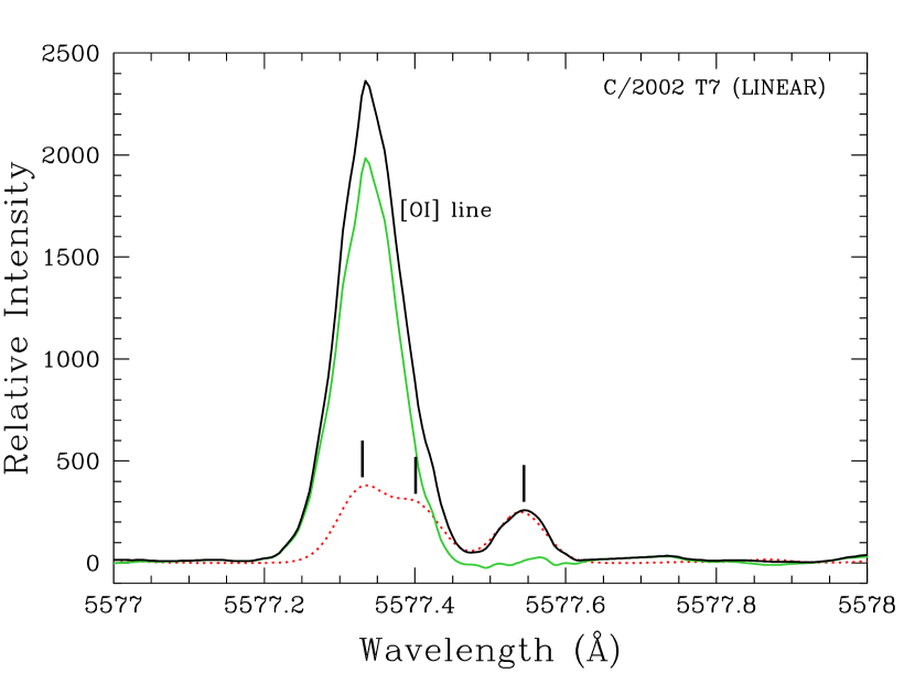
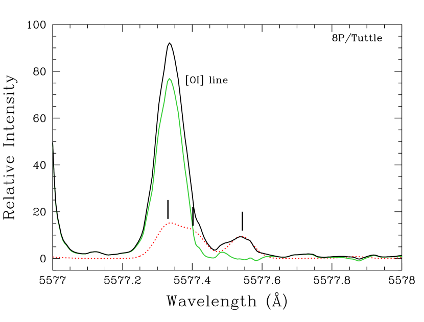
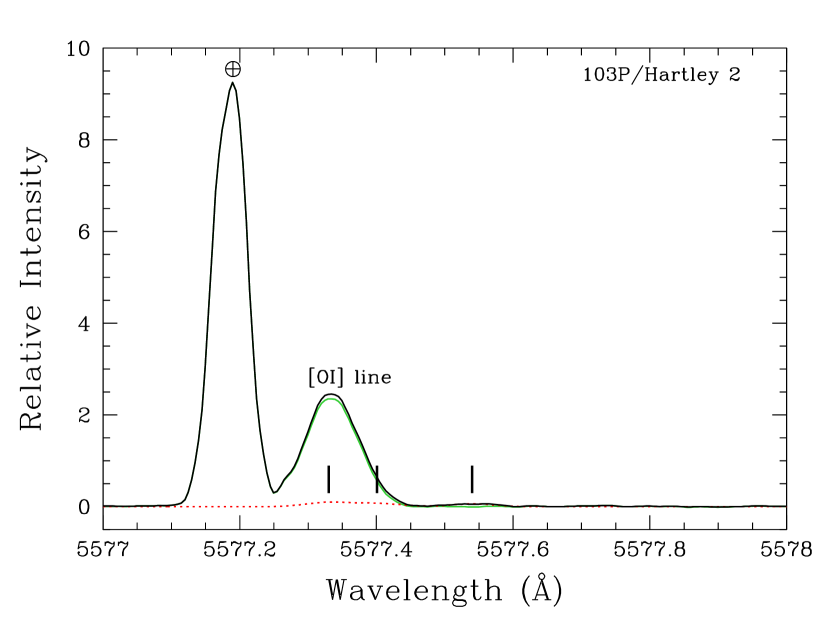
Figure 2: Subtraction of C₂ lines from the spectra of comets C/2002 T7 (LINEAR), 8P/Tuttle and 103P/Hartley 2. The black spectrum shows the data not corrected for C₂ while in the green one is after removing the C₂ lines contamination. The C₂ synthetic spectrum is represented by the dotted red line. The positions of C₂ lines at 5577.331 $\AA$, 5577.401 $\AA$ and 5577.541 $\AA$ are indicated with small vertical thick marks. The telluric [OI] line ($\oplus$) is visible in the spectrum of comet 103P/Hartley 2.

4 Results and discussion

We used the IRAF software to measure the intensities and the widths of the three [OI] lines, by making a gaussian fit.

4.1 G/R ratio

Comet	UT Date	Nucleocentric projected	Intensity (ADU)			G/R	FWHMobserved ($\AA$)			FWHMintrinsic (km s-1)
		distance range (km)	5577.339 Å	6300.304 Å	6363.776 Å		5577.339 Å	6300.304 Å	6363.776 Å	5577.339 Å	6300.304 Å	6363.776 Å
C/2002 T7 (LINEAR)	2004/05/06, 10:15	2212	3088	1015	201	0.049	0.095	0.099	0.100	2.329	1.819	1.795
	2004/05/26, 23:47	0 - 28	1899	569	426	0.172	0.096	0.090	0.091	2.634	1.759	1.734
		0 - 139	1394	425	331	0.182	0.097	0.091	0.092	2.691	1.780	1.796
		139 - 418	1576	490	317	0.154	0.099	0.090	0.093	2.747	1.734	1.836
		418 - 697	1842	560	203	0.084	0.097	0.089	0.090	2.676	1.717	1.696
		697 - 976	1523	456	139	0.070	0.095	0.088	0.090	2.623	1.644	1.713
		976 - 1784	1155	358	84	0.056	0.094	0.089	0.090	2.554	1.683	1.729
	2004/05/27, 01:06	0 - 29	1837	555	289	0.121	0.097	0.089	0.091	2.695	1.700	1.771
		0 - 143	1690	515	280	0.127	0.100	0.090	0.092	2.792	1.738	1.775
		143 - 428	1675	503	245	0.114	0.093	0.088	0.095	2.543	1.644	1.913
		428 - 714	1763	533	171	0.074	0.095	0.089	0.090	2.623	1.687	1.717
		714 - 1000	1504	450	120	0.062	0.094	0.087	0.091	2.554	1.595	1.750
		1000 - 1828	1139	345	77	0.052	0.091	0.089	0.091	2.470	1.683	1.738
	2004/05/28, 23:24	24522	47	14	4	0.065	0.088	0.100	0.096	2.043	1.822	1.610
	2004/05/29, 00:09	24522	40	12	4	0.071	0.084	0.101	0.100	1.868	1.870	1.758
73P-C/SW 3	2006/05/27, 09:31	0 - 10	712	234	189	0.200	0.107	0.109	0.108	2.278	1.493	1.369
		0 - 51	697	232	188	0.202	0.107	0.108	0.108	2.253	1.475	1.419
		51 - 153	612	202	145	0.178	0.106	0.107	0.111	2.214	1.421	1.594
		153 - 255	595	203	92	0.115	0.106	0.109	0.107	2.204	1.493	1.312
		255 - 357	519	174	64	0.092	0.105	0.107	0.105	2.143	1.396	1.211
		357 - 653	405	133	18	0.033	0.103	0.107	0.106	2.077	1.390	1.266
8P/Tuttle	2008/01/16, 01:00	0 - 25	182	61	15	0.063	0.088	0.092	0.093	2.030	1.481	1.477
		0 - 126	172	59	16	0.068	0.090	0.093	0.093	2.084	1.575	1.482
		126 - 377	162	53	11	0.052	0.090	0.093	0.094	2.106	1.551	1.517
		377 - 628	144	47	6	0.034	0.083	0.092	0.091	1.762	1.501	1.363
		628 - 1305	102	34	4	0.028	0.089	0.092	0.091	1.858	1.491	1.411
	2008/01/28, 00:58	0 - 36	547	185	68	0.093	0.089	0.094	0.094	2.068	1.584	1.544
		0 - 181	475	155	59	0.094	0.091	0.093	0.095	2.122	1.520	1.597
		181 - 544	558	185	25	0.034	0.089	0.088	0.093	2.046	1.261	1.459
		544 - 907	305	100	12	0.029	0.088	0.093	0.091	2.014	1.535	1.387
		907 - 1886	182	60	7	0.027	0.085	0.093	0.092	1.884	1.530	1.403
	2008/02/04, 00:57	0 - 43	452	149	36	0.059	0.090	0.093	0.091	2.093	1.477	1.332
		0 - 216	408	135	32	0.060	0.088	0.092	0.092	1.974	1.462	1.396
		216 - 649	465	130	23	0.039	0.089	0.088	0.091	2.038	1.238	1.348
		649 - 1081	311	101	14	0.034	0.089	0.092	0.091	2.029	1.420	1.310
		1081 - 2248	193	64	9	0.033	0.091	0.093	0.091	2.102	1.493	1.337
103P/Hartley 2	2010/11/05, 07:18	0 - 11	2.3	0.7	0.7	0.224	0.094	0.084	0.082	2.395	1.388	1.208
		0 - 54	2.1	0.7	0.7	0.240	0.095	0.084	0.086	2.432	1.413	1.428
		54 - 163	2.2	0.7	0.6	0.190	0.091	0.087	0.086	2.241	1.513	1.389
		163 - 272	2.0	0.6	0.4	0.138	0.092	0.087	0.081	2.292	1.518	1.164
		272 - 381	1.6	0.5	0.2	0.112	0.088	0.084	0.083	2.109	1.403	1.256
		381 - 696	1.3	0.4	0.2	0.094	0.084	0.083	0.084	1.955	1.328	1.324
	2010/11/05, 08:19	0 - 12	2.4	0.8	0.8	0.259	0.094	0.084	0.085	2.387	1.398	1.339
		0 - 61	2.2	0.7	0.8	0.292	0.097	0.087	0.087	2.505	1.536	1.457
		61 - 184	2.2	0.7	0.7	0.236	0.097	0.084	0.086	2.505	1.413	1.389
		184 - 306	2.0	0.7	0.4	0.167	0.092	0.087	0.080	2.308	1.518	1.119
		306 - 428	1.8	0.6	0.3	0.121	0.093	0.083	0.084	2.337	1.349	1.288
		428 - 783	1.4	0.4	0.2	0.087	0.085	0.083	0.084	1.991	1.349	1.314
	2010/11/10, 07:17	0 - 11	2.8	0.9	0.9	0.256	0.093	0.082	0.084	2.353	1.316	1.354
		0 - 54	2.4	0.8	0.9	0.288	0.092	0.084	0.083	2.312	1.396	1.267
		54 - 163	2.4	0.6	0.5	0.180	0.093	0.081	-	2.329	1.249	-
		163 - 272	2.1	0.7	0.3	0.096	0.087	0.078	0.082	2.113	1.070	1.209
		272 - 381	1.7	0.5	0.2	0.081	0.087	0.081	0.083	2.109	1.249	1.303
		381 - 696	1.2	0.4	0.1	0.067	0.083	0.082	0.082	1.915	1.286	1.241
	2010/11/10, 08:19	0 - 12	2.8	0.9	0.8	0.211	0.092	0.081	0.082	2.304	1.222	1.252
		0 - 61	2.0	0.7	0.7	0.272	0.094	0.082	0.082	2.407	1.280	1.241
		61 - 184	2.3	0.7	0.6	0.191	0.091	0.079	0.082	2.270	1.111	1.241
		184 - 306	2.3	0.7	0.3	0.111	0.088	0.081	0.080	2.148	1.270	1.097
		306 - 428	1.8	0.6	0.2	0.099	0.091	0.083	0.083	2.262	1.352	1.262
		428 - 783	1.3	0.4	0.2	0.088	0.087	0.082	0.083	2.083	1.311	1.278
	2010/11/11, 05:53	4134	0.2	0.1	0.02	0.064	0.079	0.083	0.083	1.739	1.338	1.269
	2010/11/11, 07:18	2756	0.8	0.3	0.04	0.046	0.081	0.082	0.082	1.833	1.300	1.195
	2010/11/11, 08:16	1378	0.3	0.1	0.02	0.042	0.081	0.081	0.081	1.823	1.228	1.183
	2010/11/11, 08:57	0 - 13	2.4	0.8	1.2	0.359	0.094	0.083	0.085	2.372	1.327	1.385
		0 - 65	2.0	0.7	1.1	0.417	0.096	0.083	0.090	2.442	1.327	1.600
		65 - 194	2.6	0.8	0.7	0.195	0.095	0.079	0.078	2.409	1.111	1.014
		194 - 323	1.8	0.6	0.3	0.135	0.095	0.081	0.084	2.401	1.244	1.320
		323 - 452	1.5	0.5	0.2	0.108	0.088	0.082	0.082	2.141	1.286	1.204
		452 - 827	1.1	0.4	0.1	0.089	0.088	0.082	0.082	2.137	1.296	1.252

Table 3: Average values of the G/R ratio and the intrinsic line FWHM for each spatial bin.

Comet	UT Date	N	Average nucleocentric	G/R	FWHMintrinsic(km s-1)
			distance range (km)		5577.339 $\AA$	6300.304 $\AA$	6363.776 $\AA$
C/2002 T7 (LINEAR)	2004/05/06∗	1	2212	0.049	2.329	1.819	1.795
	2004/05/26-27	2	0 - 29	0.147 $\pm$ 0.036	2.664 $\pm$ 0.043	1.730 $\pm$ 0.042	1.752 $\pm$ 0.026
		2	0 - 141	0.155 $\pm$ 0.039	2.741 $\pm$ 0.072	1.759 $\pm$ 0.030	1.785 $\pm$ 0.015
		2	141 - 423	0.134 $\pm$ 0.028	2.645 $\pm$ 0.144	1.689 $\pm$ 0.064	1.875 $\pm$ 0.054
		2	423 - 706	0.079 $\pm$ 0.007	2.649 $\pm$ 0.037	1.702 $\pm$ 0.021	1.706 $\pm$ 0.015
		2	706 - 988	0.066 $\pm$ 0.006	2.589 $\pm$ 0.048	1.620 $\pm$ 0.034	1.731 $\pm$ 0.027
		2	988 - 1806	0.054 $\pm$ 0.003	2.512 $\pm$ 0.060	1.683 $\pm$ 0.000	1.734 $\pm$ 0.006
	2004/05/28-29∗	2	24522	0.068 $\pm$ 0.004	1.955 $\pm$ 0.123	1.846 $\pm$ 0.034	1.684 $\pm$ 0.105
73P-C/SW 3	2006/05/27	1	0 - 10	0.200	2.278	1.493	1.369
		1	0 - 51	0.202	2.253	1.475	1.419
		1	51 - 153	0.178	2.214	1.421	1.594
		1	153 - 255	0.115	2.204	1.493	1.312
		1	255 - 357	0.092	2.143	1.396	1.211
		1	357 - 653	0.033	2.077	1.390	1.266
8P/Tuttle	2008/01/16-28, 02/04	3	0 - 35	0.072 $\pm$ 0.019	2.064 $\pm$ 0.032	1.514 $\pm$ 0.060	1.451 $\pm$ 0.109
		3	0 - 174	0.074 $\pm$ 0.018	2.060 $\pm$ 0.077	1.519 $\pm$ 0.057	1.492 $\pm$ 0.101
		3	174 - 523	0.042 $\pm$ 0.009	2.063 $\pm$ 0.037	1.350 $\pm$ 0.175	1.442 $\pm$ 0.086
		3	523 - 872	0.032 $\pm$ 0.003	1.935 $\pm$ 0.150	1.485 $\pm$ 0.059	1.353 $\pm$ 0.040
		3	872 - 1813	0.030 $\pm$ 0.003	1.948 $\pm$ 0.134	1.505 $\pm$ 0.022	1.383 $\pm$ 0.040
103P/Hartley 2	2010/11/05-10-11	5	0 - 12	0.262 $\pm$ 0.058	2.362 $\pm$ 0.036	1.330 $\pm$ 0.071	1.307 $\pm$ 0.074
		5	0 - 59	0.302 $\pm$ 0.068	2.420 $\pm$ 0.070	1.276 $\pm$ 0.047	1.187 $\pm$ 0.089
		5	59 - 178	0.198 $\pm$ 0.022	2.351 $\pm$ 0.107	1.279 $\pm$ 0.180	1.258 $\pm$ 0.177
		5	178 - 296	0.129 $\pm$ 0.027	2.252 $\pm$ 0.119	1.324 $\pm$ 0.193	1.182 $\pm$ 0.088
		5	296 - 414	0.104 $\pm$ 0.015	2.192 $\pm$ 0.103	1.328 $\pm$ 0.061	1.263 $\pm$ 0.038
		5	414 - 757	0.085 $\pm$ 0.010	2.016 $\pm$ 0.092	1.314 $\pm$ 0.025	1.282 $\pm$ 0.037
	2010/11/11, 05:53∗	1	4134	0.064	1.739	1.338	1.269
	2010/11/11, 07:18∗	1	2756	0.046	1.833	1.300	1.195
	2010/11/11, 08:16∗	1	1378	0.042	1.825	1.228	1.183

When collisional quenching is neglected, the intensity $I$ of an emission line, expressed in Rayleighs (R), is given theoretically by Festou & Feldman (1981) :

$$I=\leavevmode\nobreak\ \leavevmode\nobreak\ 10^{-6}\leavevmode\nobreak\ \leavevmode\nobreak\ \tau_{p}^{-1}\leavevmode\nobreak\ \leavevmode\nobreak\ \alpha\leavevmode\nobreak\ \leavevmode\nobreak\ \beta\leavevmode\nobreak\ \leavevmode\nobreak\ N$$ (1)

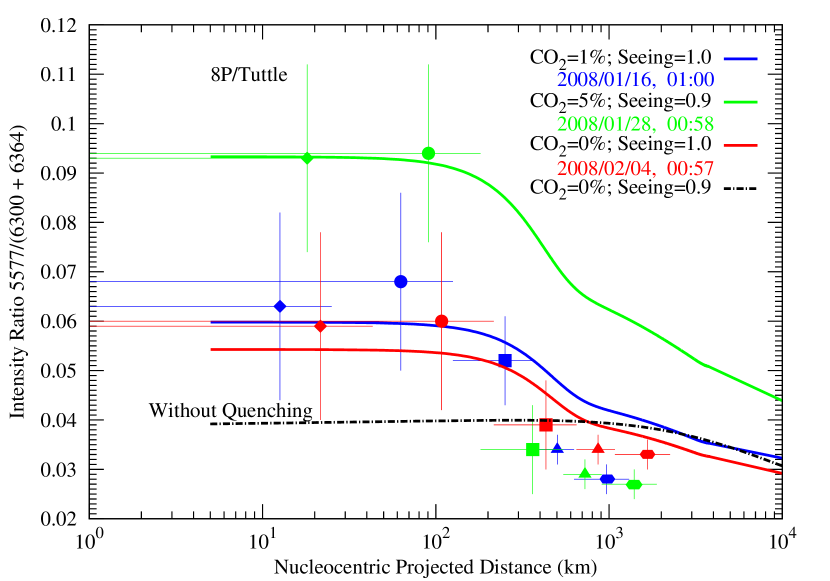
Figure 5: The G/R ratio for each sub-slit spectra for comet 8P/Tuttle. The range of nucleocentric distances covered by each point as well as the error on the G/R ratio are represented. The model calculated green to red-doublet emission intensity ratios as a function of projected distance in comet are plotted. A H₂O production rate of 1.4 $\times$ 10²⁸ s^-1 and 0.5% CO as relative abundance have been used with different seeing values and with different CO₂ relative abundances. The fits give the CO₂ relative abundance of the comet. The black dash-dotted curve represents the calculated G/R ratio accounting for no collisional quenching with 0$\%$ CO₂ relative abundance.

where $\tau_{p}$ is the photodissociative lifetime of the parent species in seconds, $\alpha$ is the yield of photodissociation, $\beta$ corresponds to the branching ratio for the transition, and $N$ is the column density of the parent species in cm^-2. The measured green and red-doublet emission intensities and the corresponding G/R ratios for each spectrum of our observations are listed in Table 4. The G/R ratio is displayed for the four comets with respect to the nucleus distance in Figures 3, 4, 5 and 6. It is given in Table 3 with the errors on the y-axis estimated from the rms of the N spectra available for a given comet. Errors on the x-axis correspond to the spatial area (in km) covered by the considered sub-slit. The atmospheric seeing limits the spatial resolution and defines a minimal nucleocentric distance that could be resolved. This minimal nucleocentric distance is provided in the last column of Table 2 and is also included in the x-axis errors. Referring to the latter figures, we notice that the G/R ratio decreases monotonically with the projected distance from the nucleus. This is due to strong collisional quenching of the excited oxygen atoms by H₂O (Bhardwaj & Raghuram, 2012). Since the lifetime of O(¹D) atoms is $\sim$100 times longer than the one of O(¹S), the destruction of O(¹D) by quenching is more important (Raghuram & Bhardwaj, 2014) and implies an increase of the G/R ratio close to the nucleus as we see in our observations. Without accounting for collisional quenching of O(¹S) and O(¹D), the model calculated G/R ratio profiles are plotted with dash-dotted curves in Figures 3 to 6. The G/R ratio is almost flat throughout the projected coma of all these comets and is significantly smaller compared to the observed values very close to the nucleus. This calculation shows the importance of the collisional quenching in determining the G/R ratio in comets. The destruction rate profiles of O(¹S) and O(¹D) by H₂O in the innermost coma depends on the size of the collisional coma of the comet which is proportional to the water production rate. The larger the H₂O production rate, the more extended the collisional coma and the stronger the quenching by H₂O molecules. That is why comet C/2002 T7 (LINEAR), with a higher Q${}_{\rm{H_{2}O}}$ $\sim$ 5 $\times$ 10²⁹ s^-1, reaches the minimal value of the G/R ratio at larger distances ($\sim$1000 km) than to the other comets ($\sim$500 km).
We also analyzed the theoretical estimates of production rates for O(¹S) and O(¹D) atoms which depend on the water production rate (Raghuram & Bhardwaj, 2013, 2014). For comets 73P-C, 8P and 103P with Q${}_{H_{2}O}$ $\sim$ 10²⁸ s^-1, O(¹S) comes both from CO₂ and H₂O while O(¹D) is only produced by the photodissociation of H₂O. However, for C/2002 T7 (LINEAR) the O(¹S) atoms are formed by the photodissociation of CO₂ close to the nucleus (¡50 km) and, beyond, by both CO₂ and H₂O. Therefore, looking at the O(¹S)/O(¹D) values in Table 1, we should expect a higher G/R ratio below 50 km for this comet. Unfortunately, the atmospheric seeing does not permit us to resolve the coma at such small distances to the nucleus. Beyond $10^{3}$ km, the main contribution to both O(¹S) and O(¹D) is the photodissociation of H₂O molecules. As shown in Figs. 3, 4, 5 and 6, at such distances, the G/R ratio reaches a constant value of $\sim$0.05 which is very close to the O(¹S)/O(¹D) value for the pure water case (cf. Table 1).

Table 4: Water production rates around the observing dates. Comets Hyakutake and Hale-Bopp included for comparison.

Comet	$r$	$Q_{H_{2}O}$ ($10^{28}$ s-1)	Date	Reference for $Q_{H_{2}O}$
C/2002 T7 (LINEAR)	0.68	35.5	2004 May 5	DiSanti et al. (2006)
	0.94	52.1	2004 May 27	Combi et al. (2009)
73P-C/Schwassmann-Wachmann 3	0.95	1.70	2006 May 17	Schleicher & Bair (2011)
8P/Tuttle	1.04	1.4	2008 Jan 3	Barber et al. (2009)
103P/Hartley 2	1.06	1.15	2010 Nov 31	Knight & Schleicher (2013)
C/1996 B2 (Hyakutake)	0.94	26	1996 Apr 1	Combi et al. (1998)
C/1995 A1 (Hale-Bopp)	0.93	957	1997 Mar 26	Dello Russo et al. (2000)

4.1.1 Estimation of CO₂ relative abundances

We used the coupled-chemistry-emission model of Bhardwaj & Raghuram (2012) to estimate the CO₂ relative abundance (i.e. the CO₂/H₂O abundance ratio) in these comets by comparing the observed slit-centered G/R data points. The model accounts for the major production and loss processes of O(¹S) and O(¹D) atoms in the inner cometary coma. This model also includes the collisional quenching of O(¹S) (4 $\times$ 10^-10 molecule^-1 cm³ s^-1, Stuhl & Welge 1969) and O(¹D) (2.1 $\times$ 10^-10 molecule^-1 cm³ s^-1, Atkinson et al. 2004; Takahashi et al. 2005) by H₂O in the inner coma. More details about the model calculations are given in Bhardwaj & Raghuram (2012); Raghuram & Bhardwaj (2013, 2014). We take the atmospheric seeing effect into account, which is especially important very close to the nucleus. For this, we convolved the spatial profile provided by the model with a gaussian of FWHM equal to the seeing value. The seeing values are obtained from the Paranal seeing monitor. The H₂O production rates and the seeing values used in the model as well as the corresponding heliocentric distances are given in Tables 2 and 4.1. The CO relative abundances for comets C/2002 T7 and 73P-C are assumed equal to 5$\%$ in the model. However, the earlier works (Bhardwaj & Haider, 2002; Raghuram & Bhardwaj, 2013, 2014) have shown that the role of CO in the determining G/R ratio is insignificant. The derived CO₂ relative abundances obtained by fitting the observed G/R profiles with the model are provided in the last column of Table 4.1.1.

The comparison between the observed and the computed G/R profiles of comet C/2002 T7 shown in Fig. 3 indicates that the relative abundance of CO₂ in this comet is less than 2%. Similarly, the computed G/R profile for comet 73P-C with 5% CO₂ relative abundance are presented in Fig. 4 together with the observations. The model calculations on comet 8P suggests that for 8P/Tuttle, the CO₂ relative abundance in this comet should be between 0 and 5%. In comet 103P (shown in Fig. 6), the required CO₂ relative abundances needed to reproduce the observations are about 15 to 20% which is in agreement with the CO₂ measurements obtained by EPOXI observations (A’Hearn et al., 2011). This is the only comet with such a high CO₂ abundance in our sample. The observed data close to the nucleus are pretty well fitted with the model calculations on all these comets, which indicates that the O(¹S) and O(¹D) collisional quenching rates measured by Stuhl & Welge (1969) and Takahashi et al. (2005) lie in a plausible range.

Table 5: The input parameters used in the model and the derived CO₂ abundances relative to H₂O.

Comet	$Q_{H_{2}O}^{a}$	$r$	Relative abundance (%)
	($10^{28}$ s-1)	(au)	[CO]	Model [CO2]
C/2002 T7 (LINEAR)	52	0.94	5b	0 - 2
73P-C/Schwassmann-Wachmann 3	1.7	0.95	5b	5
8P/Tuttle	1.4	1.03	0.5c	0 - 5
103P/Hartley 2	1.15	1.06	0.15-0.45d	15 - 20

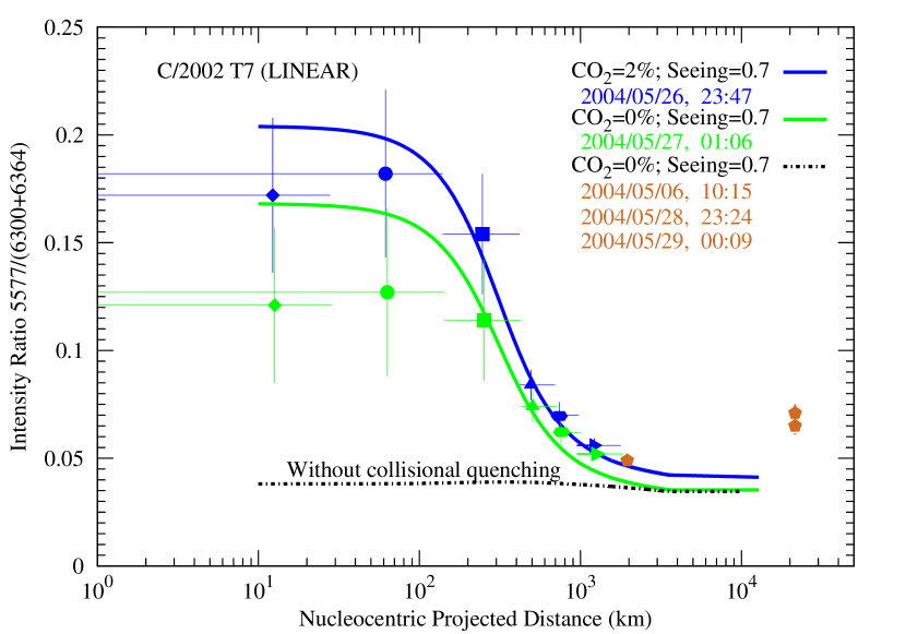
Figure 3: The G/R ratio for each sub-slit and offseted spectra for comet C/2002 T7 (LINEAR). The range of the nucleocentric distances covered by each point as well as the error on the G/R ratio are represented. The seeing is included in the x-errors and is indicated in km. It corresponds to the smallest size that can be resolved and explains the plateau found for the smallest spatial bin close to the nucleus. The calculated green to red-doublet emission intensity ratios as a function of the projected nucleocentric distance are plotted with solid curves. A H₂O production rate of 5.2 $\times$ 10²⁹ s^-1 and a 5% CO relative abundance have been used with different seeing values and with different CO₂ relative abundances. The fits give the CO₂ relative abundance of the comet. Only non offset data points are considered for the computation of the G/R profile provided by the model. The black dash-dotted curve represents the calculated G/R ratio accounting for no collisional quenching with 0% CO₂ relative abundance. The pentagon symbols are the data points for the offset observations.

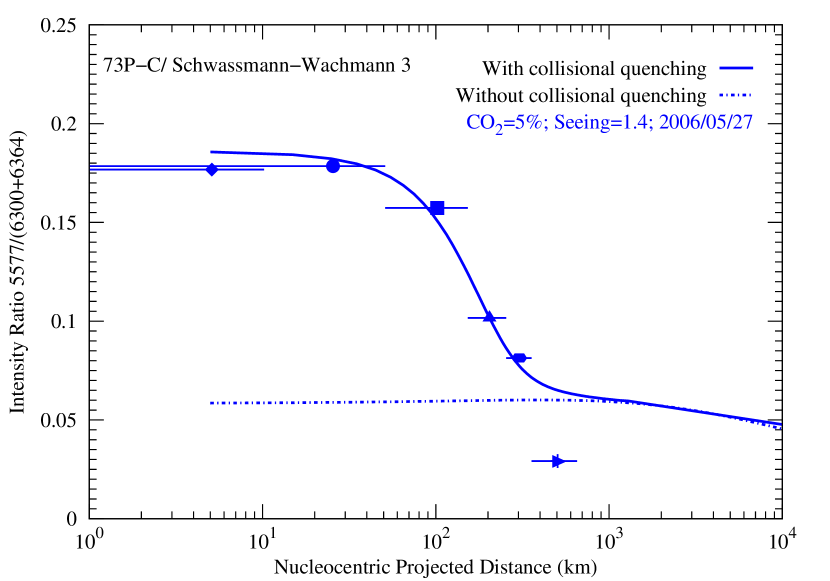
Figure 4: The G/R ratio for each sub-slit spectrum for comet 73P-C/Schwassmann-Wachmann 3. The range of nucleocentric distances covered by each point is indicated. The model calculated green to red-doublet emission intensity ratio as a function of projected distance is plotted with solid curve. A H₂O production rate of 1.7 $\times$ 10²⁸ s^-1 and 0.5% CO relative abundance have been used. The fit gives the CO₂ relative abundance of the comet. The blue dash-dotted curve represents the calculated G/R ratio accounting for no collisional quenching with 0$\%$ CO₂ relative abundance.

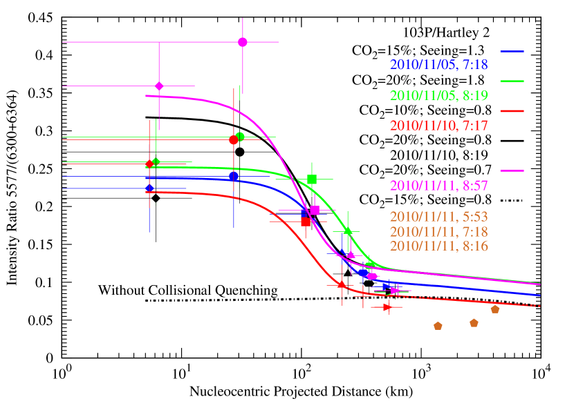
Figure 6: The G/R ratio for each sub-slit and offset spectra for comet 103P/Hartley 2. The range of nucleocentric distances covered by each point as well as the error on the G/R ratio are represented. The model calculated green to red-doublet emission intensity ratios as a function of projected distance are plotted. A H₂O production rate of 1.18 $\times$ 10²⁸ s^-1 and 0.5% CO as relative abundance have been used with different seeing values and with different CO₂ relative abundances. The fits give the CO₂ relative abundance of the comet. The black dash-dotted curve represents the calculated G/R ratio accounting for no collisional quenching with 15% CO₂ relative abundance. The pentagon symbols are the data points for the offset observations.

4.1.2 103P/Hartley 2

Two data points very close to the nucleus (observed on 2010/11/11, 8:57) appear relatively high in Fig. 6 while the other points further away from the nucleus have similar G/R values as the other spectra. First, we thought of a possible contamination by a cosmic ray but an analysis of the three [OI] lines in the 2D spectra shows no cosmic ray event (see Fig. 7). Fig. 7 also confirms that there was no problem during the acquisition of this spectrum by comparing it to the one taken the day before. This suggests that the CO₂/H₂O abundance could sometimes strongly vary close to the nucleus. These variations could be due to icy particles that evaporate very fast in the first ten kilometers and/or to the rotation of the nucleus, as it has been shown that the CO₂ is coming from a localized region (the small lobe) of the nucleus (A’Hearn et al., 2011).

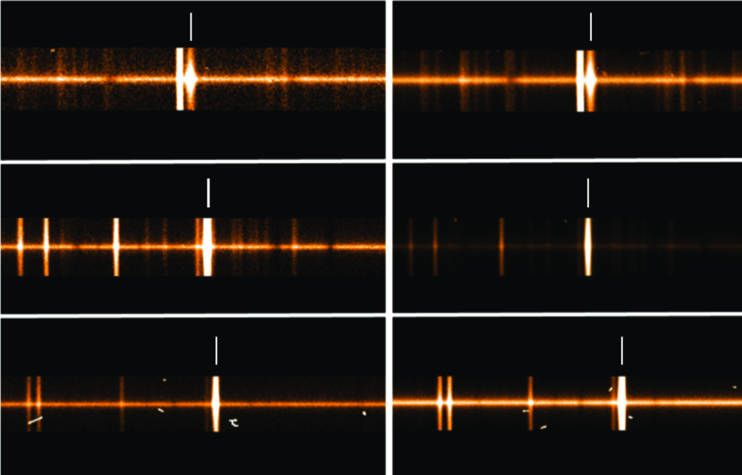
Figure 7: [OI] lines in 2D echelle spectra of 103P/Hartley 2, on 2010/11/10, 09:19 (right) and on 2010/11/11, 08:57 (left). From top to bottom, the 5577 $\AA$, 6300 $\AA$ and 6364 $\AA$ lines. The positions of the [OI] lines are indicated. No cosmic ray feature contaminates the [OI] lines.

4.2 Line widths

Using relation (9) given in Decock et al. (2013),

$$\rm{FWHM(v)}=\frac{FWHM_{intrinsic}\leavevmode\nobreak\ (\rm{\lambda})\leavevmode\nobreak\ \leavevmode\nobreak\ \rm{c}}{2\leavevmode\nobreak\ \lambda_{[OI]}\leavevmode\nobreak\ \sqrt{\ln\leavevmode\nobreak\ 2}}\leavevmode\nobreak\ ,$$ (2)

where the intrinsic line widths (FWHM($\lambda$)), corrected for the instrumental broadening, are evaluated from the measured FWHM_observed ($\AA$). The results are listed in Table 4 and the errors on the velocity widths are provided in Table 3. Figures 8, 9 and 10 plot the intrinsic width of the three forbidden oxygen lines as a function of the nucleocentric distance. In our observations, we clearly notice that the green line is wider than the red lines ($\sim$2.5 km s^-1 versus $\sim$1.5 km s^-1) even after the subtraction of the C₂ contamination. This was first noticed by Cochran (2008) and confirmed by Decock et al. (2013) for a large sample of comets. It should be emphasized that 73P-C presents, like all comets, a wider green line while this comet is very poor in C₂. Therefore, the larger width of the $5577\leavevmode\nobreak\ \r{A}$ line cannot be explained by the C₂ blends alone. A blend with another species cannot be excluded but this is unlikely. The green line width decreases when the distance to the nucleus increases (Fig. 8). This trend is more obvious for comets C/2002 T7 and 103P for which we have spectra taken at large distances from the nucleus. The green line width at large distance is also getting similar to the width of the red lines. Extrapolating the linear regression for the green line width of 103P and C/2002 T7 with the distance, we expect that the green line width will be equal to the red line width at $\sim$5000 km for 103P and $\sim$35000 km for C/2002 T7. More observations at larger distances from the nucleus are needed to confirm it. We cannot explain this behavior by the collisional quenching because this is not seen for the red lines. Indeed, as already mentioned by Raghuram & Bhardwaj (2014), the O(¹D) atoms are more quenched than the O(¹S) atoms due to their longer lifetime. Therefore, the collisional quenching should make the red line wider than the green line which is not observed. The larger width of the green line close to the nucleus could be explained by the fact that the O(¹S) atoms are mainly produced by CO₂ very close to the nucleus. Indeed, the solar flux responsible for the production of O(¹S) from CO₂ comes from the 955-1165 $\AA$ region (Bhardwaj & Raghuram, 2012) which is more energetic than the Lyman-$\alpha$ photons, supposedly considered as the main source of oxygen atom production from H₂O dissociation. These energetic photons can penetrate deeper in the thick coma than the Lyman-$\alpha$ photons. Since the line width is related to the value of the excess energy remaining after the photodissociation, an excitation by higher energetic photons produces larger widths, as we notice for the green line close to the nucleus. The excess energy of different parent molecules has been evaluated by Raghuram & Bhardwaj (2014). They found that the excess energy from CO₂ is higher than that from H₂O. When the O(¹S) atoms are observed far away from the nucleus, they are coming from both CO₂ and H₂O but with Lyman-$\alpha$ photons as the major excitation source, and then with a larger contribution from the water molecules, which results in a decrease of the green line widths.
Bisikalo et al. (2014) investigated about the larger width of the green line and provided a different explanation. They developed a Monte Carlo model to study the [OI] lines widths and suggested that the observed line profile also depends on the thermalization due to elastic collisions. Nevertheless, the thermalization process leads to a broadening of the red lines and not of the green line which is not in agreement with our observations.
In Figs. 8 to 10, we notice that the widths of the three forbidden oxygen lines of C/2002 T7 (LINEAR) are always larger than the ones of the other comets. We explain this by the higher water production rate of this comet. Indeed Tseng et al. (2007) have shown that the expansion velocity of the molecules increases when the water production rate increases.

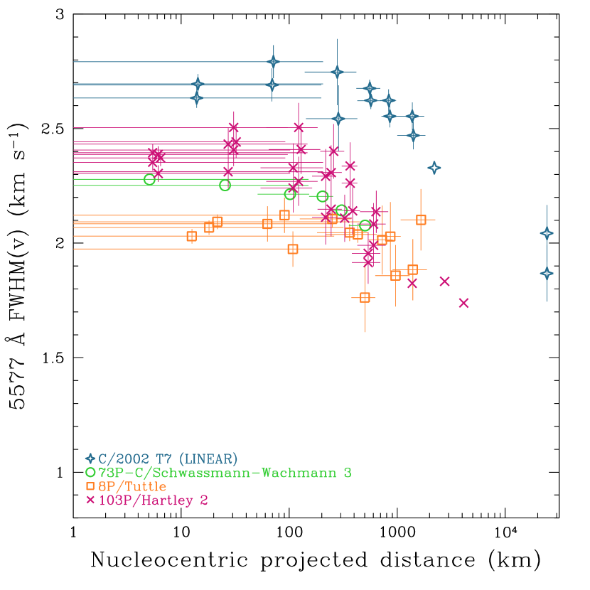
Figure 8: The 5577.339 $\AA$ line width against the distance to the nucleus for all comets. The errors on the distance and the widths are represented. A decrease of the width with the nucleocentric distance is observed for all comets. Within about 300 km, there is a plateau because of the convolution by the seeing.

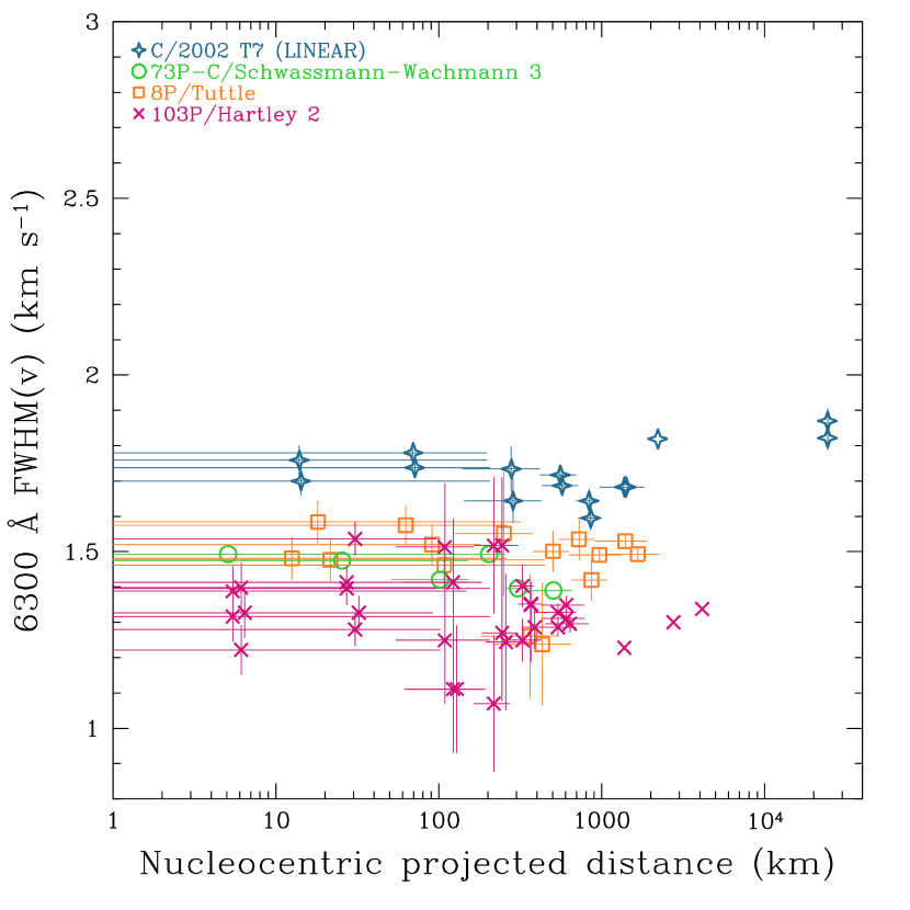
Figure 9: Same figure as Fig. 8 but for the 6300.304 $\AA$ line.

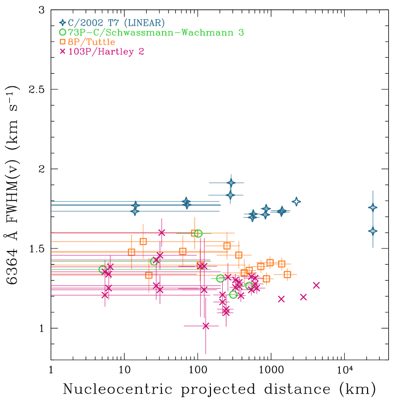
Figure 10: Same figure as Fig. 8 but for the 6363.776 $\AA$ line.

5 Conclusions

Four comets have been observed at small geocentric distances with the UVES spectrograph (VLT). 17 high-resolution spectra have been collected when the comets were very close to the Earth (¡ 0.65 au) allowing the study of the [OI] lines as close as 100 km from the nucleus. Some of them were also recorded with an offset from the nucleus corresponding to a distance of 10 000 km. The 11 centered spectra were spatially extracted and binned per pixel zones in order to get 1D spectra at various distances from the nucleus. Finally, we studied the forbidden oxygen lines in 63 sub-spectra and 6 offset spectra corresponding to different nucleocentric distances. The G/R ratio and the velocity widths have been computed and analyzed in order to better understand the production of oxygen atoms in the coma. The results can be summarized as follows :

1. In this analysis, C₂ blends have been identified and removed from the oxygen green line. This subtraction, made for the first time, is important because this contamination modifies the intensity and the FWHM of the 5577.339 $\AA$ line for comets rich in C₂ and more specifically for the analysis made far away from the nucleus. However, the C₂ blends do not explain the larger width of the green line compared to the red ones.

2. Thanks to the high spatial resolution of the data, we found that the G/R ratio as a function of the nucleocentric distance displays the same profile for all the comets: a rapid increase below 1000 km up to typically 0.2, and a constant value of about 0.05 at larger distances. The G/R value of about 0.1 found in previous studies is thus an average of the values obtained both close to the nucleus and at larger distances. This particular profile is mainly explained by the quenching which plays an important role in the destruction of O(¹D) atoms in the inner coma (¡1000 km). The parent molecules forming oxygen atoms can also contribute to this trend. Indeed, O(¹D) atoms are only formed by H₂O while O(¹S) are produced by both CO₂ and H₂O. With increasing distance from the nucleus, the relative H₂O contribution becomes larger and thus the intensity of the green line decreases. In the extended coma, oxygen atoms are only formed by the photodissociation of water molecules. The G/R value of 0.05 is in good agreement with the pure water case (Table 1).

3. We fitted our observational [OI] emission lines data with coupled-chemistry-emission model calculations. The comparison between observations and model calculations suggest that the collisional quenching of O(¹S) and O(¹D) by H₂O molecules is significant in the inner coma and cannot be neglected while determining the G/R ratio. Using the measured G/R values close to the nucleus, an estimate of the relative abundance of CO₂ could also be derived for all the comets of the sample.

4. The green line has a much larger width, typically 2.5 km s^-1 compared to 1.5 km s^-1 found for the red lines. The higher width of the green line is likely due to the involvement of different parent molecules in producing the O(¹S) and O(¹D) atoms (as already suggested by Bhardwaj & Raghuram (2012); Decock et al. (2013)): the green oxygen lines are produced by oxygen atoms coming from the photodissociation of both the CO₂ and H₂O molecules while the red ones are produced mainly by H₂O molecules. While the O(¹S) atoms are mostly provided by CO₂, the contribution of water molecules increases with the nucleocentic distance. This explains the decreasing width of the 5577.339 $\AA$ line at distances larger than 500 km.

5. Measuring the green and red-doublet emission intensities and their line widths is a new way to constrain the CO₂ relative abundances in comets.