Approximating Betweenness Centrality in Large Evolving Networks

Abstract

Betweenness centrality ranks the importance of nodes by their participation in all shortest paths of the network. Therefore computing exact betweenness values is impractical in large networks. For static networks, approximation based on randomly sampled paths has been shown to be significantly faster in practice. However, for dynamic networks, no approximation algorithm for betweenness centrality is known that improves on static recomputation. We address this deficit by proposing two incremental approximation algorithms (for weighted and unweighted connected graphs) which provide a provable guarantee on the absolute approximation error. Processing batches of edge insertions, our algorithms yield significant speedups up to a factor of $10^{4}$ compared to restarting the approximation. This is enabled by investing memory to store and efficiently update shortest paths. As a building block, we also propose an asymptotically faster algorithm for updating the SSSP problem in unweighted graphs. Our experimental study shows that our algorithms are the first to make in-memory computation of a betweenness ranking practical for million-edge semi-dynamic networks. Moreover, our results show that the accuracy is even better than the theoretical guarantees in terms of absolutes errors and the rank of nodes is well preserved, in particular for those with high betweenness.

Keywords: betweenness centrality, algorithmic network analysis, graph algorithms, approximation algorithms, shortest paths

1 Introduction

The algorithmic analysis of complex networks has become a highly active research area recently. One important task in network analysis is to rank nodes by their structural importance using centrality measures. Betweenness centrality (BC) measures the participation of a node in the shortest paths of the network. Let the graph $G$ represent a network with $n$ nodes and $m$ edges. Naming $\sigma_{st}$ the number of shortest paths from a node $s$ to a node $t$ and $\sigma_{st}(v)$ the number of shortest paths from $s$ to $t$ that go through $v$, the (normalized) BC of $v$ is defined as [9]: $c_{B}(v)=\frac{1}{n(n-1)}\sum_{s\neq v\neq t}\frac{\sigma_{st}(v)}{\sigma_{st}}$. Nodes with high betweenness can be important in routing, spreading processes and mediation of interactions. Depending on the context, this can mean, for example, finding the most influential persons in a social network, the key infrastructure nodes in the internet, or super spreaders of a disease.

The fastest existing method for computing BC is due to Brandes [4]. It requires $\Theta(nm)$ operations for unweighted graphs and $\Theta(nm+n^{2}\log n)$ for graphs with positive edge weights. This time complexity is prohibitive for large-scale graphs with millions of edges, though. Recent years have seen the publication of several ap proximation algorithms that aim to reduce the computational effort, while finding BC values that are as close as possible to the exact ones. Good results have been obtained in this regard; in particular, a recent algorithm by Riondato and Kornaropoulos (RK) [21] gives probabilistic guarantees on the quality of the approximation, and we build our algorithms on this method.

Motivation.

Large graphs of interest, such as the Web and social networks, evolve continuously. Thus, in addition to the identification of important nodes in a static network, an issue of great interest is the evolution of centrality values in dynamically changing networks. So far, there are no approximation algorithms that efficiently update BC scores rather than recomputing them from scratch. A few methods have been proposed to update the BC values after a graph modification, which for some of the algorithms can only be one edge insertion and for others can also be one edge deletion. However, all of these approaches are exact and have a worst-case time complexity which is the same as Brandes’s algorithm (BA) [4] and a memory footprint of at least $O(n^{2})$.

Contribution.

In this paper, we present the first approximation algorithms for BC in evolving networks. They are the first incremental algorithms (i. e. they update the betweenness values of all nodes in response to edge insertions or weight decrease operations in the graph) that can actually be used in large streaming graphs. Our two algorithms IA (for incremental approximation) and IAW (for IA weighted) work for unweighted and weighted networks, respectively. Even though only edge insertions and weight decreases are supported as dynamic operations, we do not consider this a major limitation since many real-world dynamic networks evolve only this way and do not shrink. The algorithms we propose are also the first that can handle a batch of edge insertions (or weight decrease operations) at once. After each batch of updates, we guarantee that the approximated BC values differ by at most $\epsilon$ from the exact values with probability at least $1-\delta$, where $\epsilon$ and $\delta$ can be arbitrarily small constants. Running time and memory required depend on how tightly the error should be bounded. As part of our algorithm IA, we also propose a new algorithm with lower time complexity for updating single-source shortest paths in unweighted graphs after a batch of edge insertions.

Our experimental study shows that our algorithms are the first to make in-memory computation of a betweenness ranking practical for large dynamic networks. For comparison, we create and evaluate the first implementation of the dynamic BC algorithm by Nasre et al. [18] and observe its lack of speedup and scalability. We achieve a much improved scaling behavior, enabling us to update approximate betweenness scores in a network with 16 million edges in a few seconds on typical workstation hardware, where previously proposed dynamic algorithms for betweenness would fail by their memory requirements alone. More generally, processing batches of edge insertions, our algorithms yield significant speedups (up to factor $10^{4}$) compared to restarting the approximation. Regarding accuracy, our experiments show that the estimated absolute errors are always lower than the guaranteed ones. Also the rank of nodes is well preserved, in particular for those with high betweenness.

2 Related work

Static BC algorithms - exact and approximation.

The fastest existing method for the exact BC computation, BA, requires $\Theta(nm)$ operations for unweighted graphs and $\Theta(nm+n^{2}\log n)$ for graphs with positive edge weights [4]. The algorithm computes for every node $s\in V$ a slightly-modified version of a single-source shortest-path tree (SSSP tree), producing for each $s$ the directed acyclic graph (DAG) of all shortest paths starting at $s$. Exploiting the information contained in the DAGs, the algorithm computes the dependency $\delta_{s}(v)$ for each node $v$, that is the sum over all nodes $t$ of the fraction of shortest paths between $s$ and $t$ that $v$ is internal to. The betweenness of each node $v$ is simply the sum over all sources $s\in V$ of the dependencies $\delta_{s}(v)$. Therefore, we can see the dependency $\delta_{s}(v)$ as a contribution that $s$ gives to the computation of $c_{B}(v)$. Based on this concept, some algorithms for an approximation of BC have been developed. Brandes and Pich [5] propose to approximate $c_{B}(v)$ by extrapolating it from the contributions of a subset of source nodes, also called pivots. Selecting the pivots uniformly at random, the approximation can be proven to be an unbiased estimator for $c_{B}(v)$ (i.e.  its expectation is equal to $c_{B}(v)$). In a subsequent work, Geisberger et al. [13] notice that this can produce an overestimation of BC scores of nodes that happen to be close to the sampled pivots. To limit this bias, they introduce a scaling function which gives less importance to contributions from pivots that are close to the node. Bader et al. [1] approximate the BC of a specific node only, based on an adaptive sampling technique that reduces the number of pivots for nodes with high centrality. Different from the previous approaches is the approximation algorithm of Riondato and Kornaropoulos [21], which samples a single random shortest path at each iteration. This approach allows theoretical guarantees on the quality of their approximation: For any two constants $\epsilon,\delta\in(0,1)$, a number of samples can be defined such that the error on the approximated values is at most $\epsilon$ with probability at least $1-\delta$. Because of this guarantee, we use this algorithm as a building block of our new approach and refer to it as RK.

Exact dynamic algorithms.

Dynamic algorithms update the betweenness values of all nodes in response to a modification on the graph, which might be an edge insertion, an edge deletion or a change in an edge’s weight. The first published approach is QUBE by Lee et al. [15], which relies on the decomposition of the graph into connected components. When an edge update occurs, QUBE re-computes the centrality values using BA only within the affected component. In case the update modifies the decomposition, this must be recomputed, and new centralities must be calculated for all affected components. The approach proposed by Green et al. [14] for unweighted graphs maintains a structure with the previously calculated BC values and additional information, like the distance of each node $v$ from every source $s\in V$ and the list of predecessors, i.e. the nodes immediately preceding $v$ in all shortest paths from $s$ to $v$. Using this information, the algorithm tries to limit the recomputations to the nodes whose betweenness has actually been affected. Kourtellis et al. [17] modify the approach by Green et al. [14] in order to reduce the memory requirements. Instead of storing the predecessors of each node $v$ from each possible source, they recompute them every time the information is required. Kas et al. [16] extend an existing algorithm for the dynamic APSP problem by Ramalingam and Reps [19] to also update BC scores. The recent work by Nasre et al. [18] contains the first dynamic algorithm for BC (NPR) which is asymptotically faster than recomputing from scratch on certain inputs. In particular, when only edge insertions are allowed and the considered graph is sparse and weighted, their algorithm takes $O(n^{2})$ operations, whereas BA requires $O(n^{2}\log n)$ on sparse weighted graphs. Among other things, our paper contains the first experimental results obtained by an implementation of this algorithm.

All dynamic algorithms mentioned perform better than recomputation on certain inputs. Yet, none of them has a worst-case complexity better than BA on all graphs since all require an update of an APSP problem. For this problem, no algorithm exists which has better worst-case running time than recomputation [22]. In addition, the problem of updating BC seems even harder than the dynamic APSP problem. Indeed, the dependencies (and therefore BC) might need to be updated even on nodes whose distance from the source has not changed, as they could be part of new shortest paths or not be part of old shortest paths any more.

Dynamic SSSP algorithms.

Since our algorithms require the update of an SSSP solution, we briefly review also the main results on the incremental SSSP problem (i.e.  the problem of updating distances from a source node after an edge insertion or a batch of edge insertions). The most well-known algorithms for single-edge updates are RR [20] by Ramalingam and Reps, and FMN [11] by Frigioni et al. The two approaches are implemented and compared in [10], showing that RR is the faster one. For the batch problem, the authors of  [19] propose a novel algorithm named SWSF-FP. In [12] a batch variant of FMN is presented. The experimental analysis by Bauer and Wagner [3] reports the results of the two algorithms and of some tuned variants of SWSF-FP. The recent study by D’Andrea et al. [7] compares the performances of the algorithms considered in [3] with those of a novel approach [6]. In particular, for batches of only edge insertions, the tuned variant T-SWSF has shown significantly better results than other published algorithms. Therefore we use T-SWSF as a building block of our incremental BC approximation algorithm.

3 RK algorithm

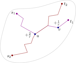
Figure 1: Sampled paths and score update in the RK algorithm

In this section we briefly describe the algorithm by Riondato and Kornaropoulos (RK) [21], the foundation for our incremental approach. The idea of RK is to sample a set $S=\{p_{(1)},...,p_{(r)}\}$ of $r$ shortest paths between randomly sampled source-target pairs $(s,t)$. Then, RK computes the approximated betweenness centrality $\tilde{c}_{B}(v)$ of a node $v$ as the fraction of sampled paths $p_{(k)}\in S$ that $v$ is internal to, by adding $\frac{1}{r}$ to the node’s score for each of these paths. Figure 1 illustrates an example where the sampling of two shortest paths leads to $\frac{2}{r}$ and $\frac{1}{r}$ being added to the score of $u$ and $v$, respectively. Each possible shortest path $p_{st}$ has the following probability of being sampled in each of the $r$ iterations:

$$\pi_{G}(p_{st})=\frac{1}{n(n-1)}\cdot\frac{1}{\sigma_{st}}$$ (1)

The number $r$ of samples required to approximate BC scores with the given error guarantee is calculated as

$$r=\frac{c}{\epsilon^{2}}\left(\lfloor\log_{2}\left(VD(G)-2\right)\rfloor+1+\ln\frac{1}{\delta}\right),$$ (2)

where $\epsilon$ and $\delta$ are constants in $(0,1)$, $c\approx 0.5$ and $VD(G)$ is the vertex diameter of $G$, i.e. the number of nodes in the shortest path of $G$ with maximum number of nodes. In unweighted graphs $VD(G)$ coincides with diam$(G)+1$, where diam$(G)$ is the number of edges in the longest shortest path. In weighted graphs $VD(G)$ and the (weighted) diameter diam$(G)$ (i. e. the length of the longest shortest path) are unrelated quantities. The following error guarantee holds:

Lemma 1

[21] If $r$ shortest paths are sampled according to the above-defined probability distribution $\pi_{G}$, then with probability at least $1-\delta$ the approximations $\tilde{c}_{B}(v)$ of the betweenness centralities are within $\epsilon$ from their exact value: $\Pr(\exists v\in V\>s.t.\>|c_{B}(v)-\tilde{c}_{B}(v)|>\epsilon)<\delta.$

To sample the shortest paths according to $\pi_{G}$, RK first chooses a node pair $(s,t)$ uniformly at random and performs an SSSP search from $s$, keeping also track of the number $\sigma_{sv}$ of shortest paths from $s$ to $v$ and of the list of predecessors $P_{s}(v)$ for any node $v$. Then one shortest path is selected: Starting from $t$, a predecessor $z\in P_{s}(t)$ is selected with probability $\sigma_{sz}/\sum_{w\in P_{s}(t)}\sigma_{sw}=\sigma_{sz}/\sigma_{st}$. The sampling is repeated iteratively until node $s$ is reached. Algorithm 2 in the Appendix is the pseudocode for RK. Function computeExtendedSSSP is an SSSP algorithm that keeps track of the number of shortest paths and of the list of predecessors while computing distances, as in BA [4].

Approximating the vertex diameter.

The authors of RK propose two upper bounds on the vertex diameter that can both be computed in $O(n+m)$, instead of solving an APSP problem. For connected unweighted undirected graphs, they compute a SSSP from a randomly-chosen node $s$ and approximate $VD$ as the sum of the two shortest paths starting from $s$ with maximum length. For the remaining graph classes (directed and/or weighted), the authors approximate $VD$ with the size of the largest weakly connected component, which, in case of connected graphs, is equal to the number of nodes, an overestimation for complex networks. It is important to note that, when the graph is connected and only edge insertions are allowed, the size of both approximations cannot increase as the graph evolves. This is the key observation on which our method relies.

4 Incremental approximation algorithms

4.1 Update after a batch

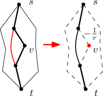
Figure 2: Updating shortest paths and BC scores

Our incremental algorithms are composed of two phases: an initialization phase, which executes RK on the initial graph, and an update phase, which recomputes the approximated BC scores after a sequence of edge updates. Figure 2 shows an example to illustrate the basic idea: Several shortest $(s,t)$-paths exist, of which one has been sampled. An edge insertion shortens the distance between $s$ and $t$, making the shortest path unique and excluding the node $v$, from whose score $\frac{1}{r}$ must be subtracted. From this point on, we give a formal description and only consider edge insertions. We suppose the graph is undirected, but our results can be easily extended to weight decreases and directed graphs. A batch $\beta=\{e_{1},...,e_{k}\}$ of edges $e_{i}=\{u_{i},v_{i}\}$ is inserted into a connected graph $G$ and we show how the approximated BC scores can be updated. Let $G^{\prime}=(V,E\cup\beta)$ be the new graph, let $d^{\prime}_{s}(t)$ denote the new distance between any node pair $(s,t)$ and let $\sigma^{\prime}_{st}$ be the new number of shortest paths between $s$ and $t$. Let $\mathcal{S}_{st}$ and $\mathcal{S}^{\prime}_{st}$ be the old and the new set of shortest paths between $s$ and $t$, respectively. A new set $S^{\prime}=\{p^{\prime}_{(1)},...,p^{\prime}_{(r)}\}$ of shortest paths has to be sampled now in order to let Lemma 1 hold for the new configuration; in particular, the probability $\Pr(p^{\prime}_{(k)}=p^{\prime}_{st})$ of each shortest path $p^{\prime}_{st}$ to be sampled must be equal to $\pi_{G^{\prime}}(p^{\prime}_{st})=\frac{1}{n(n-1)}\cdot\frac{1}{\sigma^{\prime}_{st}}$. Clearly, one could rerun RK on the new graph, but we can be more efficient: We recall that the upper bound on the vertex diameter, and therefore the number $r$ of samples, cannot increase after the insertion if the graph is connected. Given any old sampled path $p_{st}$, we can keep $p_{st}$ if the set of shortest paths between $s$ and $t$ has not changed, and replace it with a new path between $s$ and $t$ otherwise. Then, the following lemma holds:

Lemma 2

Let $S$ be a set of shortest paths of $G$ sampled according to $\pi_{G}$. Let $\mathcal{P}$ be the procedure that creates $S^{\prime}$ by substituting each path $p_{st}\in S$ with a path $p^{\prime}_{st}$ according to the following rules:

1. $p^{\prime}_{st}=p_{st}$ if $d^{\prime}_{s}(t)=d_{s}(t)$ and $\sigma^{\prime}_{st}=\sigma_{st}$

2. $p^{\prime}_{st}$ selected uniformly at random among $\mathcal{S}^{\prime}_{st}$ otherwise.

Then, $p^{\prime}_{st}$ is a shortest path of $G^{\prime}$ and the probability of any shortest path $p^{\prime}_{xy}$ of $G^{\prime}$ to be sampled at each iteration is $\pi_{G^{\prime}}(p^{\prime}_{xy})$, i.e.

$$\Pr(p^{\prime}_{(k)}=p^{\prime}_{xy})=\frac{1}{n(n-1)}\cdot\frac{1}{\sigma^{\prime}_{xy}},\quad k=1,...,r\text{ .}$$

The proof can be found in Section 0.A of the Appendix. Since the set of paths is constructed according to $\pi_{G^{\prime}}$, Theorem 4.1 follows directly from Lemma 1.

Theorem 4.1

Let $G=(V,E)$ be a connected graph and let $G^{\prime}=(V,E\cup\beta)$ be the modified graph after the insertion of the batch $\beta$. Let $S$ be a set of $r$ shortest paths of $G$ sampled according to $\pi_{G}$ and $r=\frac{c}{\epsilon^{2}}\left(\lfloor\log_{2}\left(VD(G)-2\right)\rfloor+1+\ln\frac{1}{\delta}\right)$ for some constants $\epsilon,\delta\in(0,1)$. Then, if a new set $S^{\prime}$ of shortest paths of $G^{\prime}$ is built according to procedure $\mathcal{P}$ and the approximated values of betweenness centrality $\tilde{c}^{\prime}_{B}(v)$ of each node $v$ are computed as the fraction of paths of $S^{\prime}$ that $v$ is internal to, then

$$\Pr(\exists v\in V\>s.t.\>|c^{\prime}_{B}(v)-\tilde{c}^{\prime}_{B}(v)|>\epsilon)<\delta,$$

where $c^{\prime}_{B}(v)$ is the new exact value of betweenness centrality of $v$ after the edge insertion.

Algorithm 1 shows the update procedure based on Theorem 4.1. For each sampled node pair $(s_{i},t_{i}),\,i=1,...,r$, we first update the SSSP DAG, a step which will be discussed in Section 4.2. In case the distance or the number of shortest paths between $s_{i}$ and $t_{i}$ has changed, a new shortest path is sampled uniformly as in RK. This means that $\frac{1}{r}$ is subtracted from the score of each node in the old shortest path and the same quantity is added to the nodes in the new shortest path. On the other hand, if both distances and number of shortest paths between $s_{i}$ and $t_{i}$ have not changed, nothing needs to be updated.

Considering edges in a batch allows us to recompute the BC scores only once instead of doing it after each single edge update. Moreover, this gives us the possibility to use specific batch algorithms for the update of the SSSP DAGs, which process the nodes affected by multiple edges of $\beta$ only once, instead of for each single edge.

Input : Graph $G=(V,E)$, source node $s$, number of iterations $r$, batch $\beta$

Output : New approximated BC values of nodes in $V$

1 for $i\leftarrow 1$ to $r$ do

2       $d^{old}_{i}\leftarrow d_{s_{i}}(t_{i})$;

3       $\sigma^{old}_{i}\leftarrow\sigma_{s_{i}}(t_{i})$;

4       $(d_{s_{i}},\sigma_{s_{i}},P_{s_{i}})\leftarrow$UpdateSSSP($G,d_{s_{i}},\sigma_{s_{i}},P_{s_{i}},\beta$);

       // If the shortest paths between $s_{i}$ and $t_{i}$ have changed, we sample a new one

5       if $d_{s_{i}}(t_{i})<d^{old}_{i}$ or $\sigma_{s_{i}}(t_{i})\neq\sigma^{old}_{i}$ then

             // We subtract $1/r$ from all nodes in the old shortest path and we add $1/r$ to all nodes in the new shortest path

6             foreach $w\in p_{(i)}$ do

7                   $\tilde{c}_{B}$ ($w$) $\leftarrow\textnormal{{$\tilde{c}_{B}$}}(w)-1/r$;

8                  

9             end foreach

10            $v\leftarrow t_{i}$;

11             $p_{(i)}\leftarrow$ empty list;

12             while $P_{s_{i}}(v)\neq\{s_{i}\}$ do

13                   sample $z\in P_{s_{i}}(v)$ with $\Pr=\sigma_{s_{i}}(z)/\sigma_{s_{i}}(v)$;

14                   $\textnormal{{$\tilde{c}_{B}$}}(z)\leftarrow\textnormal{{$\tilde{c}_{B}$}}(z)+1/r$;

15                   add $z$ to $p_{(i)}$;

16                   $v\leftarrow z$;

17                  

18             end while

19            

20       end if

21      

22 end for

return $\{(v,\textnormal{{$\tilde{c}_{B}$}}(v)),\>v\in V\}$

Algorithm 1 BC update after a batch $\beta$ of edge insertions

4.2 SSSP Update Algorithms

In Line 1 of Algorithm 1, we need an algorithm UpdateSSSP to update the information about distances, predecessors and number of shortest paths. This is an extension to the problem of updating a SSSP tree, for which some approaches have been proposed in the literature (see Section 2). For weighted graphs, we build our UpdateSSSP algorithm upon T-SWSF [3]; given that no existing algorithm for the dynamic SSSP is asymptotically better than recomputing from scratch, we base our choice on the results of the experimental studies [3, 7]. The difference between our UpdateSSSP for weighted graphs (UpdateSSSPW) and T-SWSF is that we also need to update the list of predecessors and the number of shortest paths in addition to the distances. For unweighted graphs, our UpdateSSSP is a novel batch SSSP update approach which is in principle similar to T-SWSF but has better time bounds. In particular, naming $||A$|| the sum of the number of nodes affected by the batch (i. e. nodes whose distance or number of shortest paths from the source has changed) and the number of their incident edges and naming $\beta$ the size of the batch, our algorithm for unweighted graphs requires $O(|\beta|+||A||+d_{max})$ for an update, where $d_{max}$ is at most equal to the vertex diameter. The time required by UpdateSSSPW (and T-SWSF) is instead $O(|\beta|\log|\beta|+||A||\log||A||)$. Our two algorithms UpdateSSSPW and UpdateSSSP lead to two incremental BC approximation algorithms: IAW, which uses UpdateSSSPW, and IA, which uses UpdateSSSP.

SSSP update for weighted graphs.

Now we briefly describe UpdateSSSPW (Algorithm 3 in Section 0.B), which is responsible for updating distances, list of predecessors and number of shortest paths in weighted graphs after a batch of edge insertions. We say we relax an edge $\{u,v\}$ when we compare $d(v)$ with $d(u)+\mathsf{w}(\{u,v\})$ and, in case $d(v)>d(u)+\mathsf{w}(\{u,v\})$, we insert $v$ in a priority queue $Q$ with priority $p_{Q}(v)=d(u)+\mathsf{w}(\{u,v\})$ (and the same swapping $u$ and $v$). Our algorithm (and T-SWSF) can be divided into two parts: In the first part (Lines 3 - 3), it relaxes all the edges of the batch. In the second part (Lines 3 - 3), each node $w$ in $Q$ is extracted, $d(w)$ is set to $p_{Q}(w)$ and all the incident edges of $w$ are relaxed. The algorithm continues until $Q$ is empty and therefore no node needs to be updated.

In this high-level structure, our algorithm is equal to T-SWSF. However, our UpdateSSSPW algorithm needs to recompute also the information about the shortest paths. This is accomplished during the scan of the incident edges: In Lines 3 - 3, we recompute the list of predecessors of node $w$ as the set of neighbors whose distance is lower than the distance of $w$. The number of shortest paths is then recomputed as the sum of the number of shortest paths of the predecessors. To study the complexity of UpdateSSSPW, we denote by $\beta$ the set of edges of the batch and by $A$ the set of affected nodes (i.e.  vertices whose distance or number of shortest paths from the source has changed as a consequence of the batch). Let $|A|$ and $|\beta|$ represent the cardinality of $A$ and $\beta$, respectively. Moreover, let $||A||$ represent the sum of the nodes in $A$ and of the edges that have at least one endpoint in $A$. Then, the following theorem holds.

Theorem 4.2

The time required by UpdateSSSPW to update the distances, the number of shortest paths and the list of predecessors is $O(|\beta|\log|\beta|+||A||\log||A||)$.

Proof

In Lines 3 - 3 of Algorithm 3, we scan all $|\beta|$ elements of the batch and perform at most one heap operation (insertion or decrease-key) for each of them, consequently requiring $O(|\beta|\log|\beta|)$ time. In the main loop (Lines 3 - 3), each affected node is extracted from $Q$ exactly once and its neighbors are scanned (and possibly inserted/updated within $Q$). This leads to a $O(||A||\log||A||)$ complexity for the main loop. The total time required by the algorithm is therefore $O(|\beta|\log|\beta|+||A||\log||A||)$.

A new SSSP update algorithm for unweighted graphs.

In case of unweighted graphs, we present a new algorithm (Algorithm 4 of Section 0.B) that can update the data structures with less computational effort than updateSSSPW. Since in unweighted graphs the distances from the source can only be discrete, we can see these distances as levels, which range from $0$ (the source) to the distance $d_{max}$ of the furthest node from the source. Therefore, we can replace the priority queue $Q$ of Algorithm 3 with a list of FIFO queues containing, for each level $k$, the affected nodes that would have priority $k$ in $Q$. As in Algorithm 3, we first scan all the edges of the batch (Lines 4 - 4), inserting the affected nodes in the queues. Then (Lines 4 - 4), we scan the queues in order of increasing distance from the source, in a similar way to the extraction of nodes from the priority queue. Also in this case, we scan the incident edges to find the new predecessors (and therefore update the list of predecessors and the number of shortest paths) (Lines 4 - 4) and to detect other possibly affected nodes (Lines 4 - 4). In order not to insert a node in the queues multiple times, we use colors. At the beginning, all the nodes are white; then, the first time a node is scanned and inserted into a queue, we set its color to gray, meaning that the node should not be inserted into a queue any more. However, the target nodes of the batch might need to be inserted in a queue more than once. Indeed, it is possible that we initially insert node $v$ at level $d_{s}(u)+1$, but then we find a shorter path during the main loop (or afterwards in the batch). For this reason, we also define another color, black, meaning that the node should not be processed any more, even if it is found again in a priority queue. Using the same notation introduced with UpdateSSSP for weighted graphs, the following theorem holds.

Theorem 4.3

The time required by UpdateSSSP to update the distances, the number of shortest paths and the list of predecessors is $O(|\beta|+||A||+d_{max})$.

Proof

The complexity of the initialization step (Lines 4 - 4) of Algorithm 4 is $O(d_{max}+|\beta|)$, as we initialize a vector of empty lists of size $d_{max}$ and scan the batch. In the main loop, we scan again the list of queues of size $d_{max}$ and, for every node $w$ in one of the queues, we scan all the incident edges of $w$. Therefore, the complexity of the main loop is the sum of the number of nodes in each queue plus the number of edges that have one endpoint in one of the queues. Using the coloring, each affected node which is not the target of an edge of the batch is inserted in $Q$ exactly once. The affected target nodes $v$, instead, can be inserted at most $n_{v}+1$ times, where $n_{v}$ is the number of edges in $\beta$ whose target is $v$. The reason of the $+1$ is that $v$ can be inserted in a queue at most once during the main loop, as then $color[v]$ will be set to gray. The complexity of the algorithm is therefore $O(|\beta|+\|A\|+d_{max})$.

5 Experiments

5.1 Experimental setup

Implementation and settings.

For an experimental comparison, we implemented our two incremental approaches IA and IAW, as well as the static approximation RK, the static exact BA, the dynamic exact algorithms GMB [14] and KDB [17] for unweighted graphs and the dynamic exact algorithm NPR [18] for weighted graphs. We chose to implement NPR because it is the only algorithm with a lower complexity than recomputing from scratch and no experimental results have been provided before. In addition, we also implemented GMB and KDB because they are the ones with the best speedups on unweighted graphs. We implemented all algorithms in C++, building on the open-source NetworKit framework [23]. In all experiments we fix $\delta$ to 0.1 while the error bound $\epsilon$ varies. The machine used has 2 x 8 Intel(R) Xeon(R) E5-2680 cores at 2.7 GHz, of which we use only one, and 256 GB RAM. All computations are sequential to make the comparison to previous work more meaningful.

Data sets.

We use both real-world and synthetic networks. In case of disconnected graphs, we extract the largest connected component first. The properties of real-world networks are summarised in Table 1. We cover a range from relatively small networks, on which we test all the implemented algorithms, to large networks with millions of edges, on which we can execute only the most scalable methods, i.e. RK and our incremental approach. In particular, the introduction of approximation allows us to approach graphs of several orders of magnitude larger than those considered by previous dynamic algorithms [17]. Our test set includes routing/transportation networks in which BC has a straightforward interpretation, as well as social networks in which BC can be understood as a measure of social influence. Most networks are publicly available from the collection compiled for the 10th DIMACS challenge [2]. Due to a shortage of actual dynamic network data with only edge dynamics, we simulate dynamics on these real networks by removing a small fraction of random edges (without separating the connected component) and adding them back in batches. To study the scalability of the methods, we also use synthetic graphs of growing sizes obtained with the Dorogovtsev-Mendes generator, a simple and scalable model for networks with power-law degree distribution [8]. Since NPR and our IAW perform best on weighted graphs, we also generate weighted instances of Dorogovtsev-Mendes networks, by adding random weights to the edges according to a Gaussian distribution with mean 1 and standard deviation 0.1.

Graph	Type	Nodes	Edges	Diameter
PGPgiantcompo	social / web of trust	10 680	24 316	(24, 24)
as-22july06	power grid	22 963	48 436	(11, 12)
caidaRouterLevel	internet	192 244	609 066	(26, 28)
email-Enron	social / communication	36 692	183 831	(13, 14)
coAuthorsCiteseer	social / coauthorship	227 320	814 134	(33, 36)
coAuthorsDBLP	social / coauthorship	299 067	977 676	(24, 26)
citationCiteseer	citations	268 495	1 156 647	(36, 38)
belgium.osm	street	1 441 295	1 549 970	(1987, 2184)
Texas84.facebook	social / friendship	36 371	1 590 655	(7,7)
netherlands.osm	street	2 216 688	2 441 238	(2553, 2808)
coPapersCiteseer	social / coauthorship	434 102	16 036 720	(34, 36)
coPapersDBLP	social / coauthorship	540 486	15 245 729	(23, 24)

Table 1: Overview of largest components of real graphs used in the experiments.

5.2 Accuracy

We consider the accuracy of the approximated centrality scores both in terms of absolute error and, more importantly, the preservation of the ranking order of nodes. Our incremental algorithm has exactly the same accuracy as RK. The authors of [21] study the behavior of the algorithm also experimentally, considering the average and maximum estimation error on a small set of real graphs. We study the absolute and relative errors (i. e. ratio between the approximated and the exact score) on a wider set of graphs. For our experiments we use PGPgiantcompo, as-22july06 and Dorogovtsev-Mendes graphs of several sizes. Our results confirm those of [21] in the sense that the measured absolute errors are always below the guaranteed maximum error $\epsilon$ and the measured average error is orders of magnitude smaller than $\epsilon$. We observe that the relative error is almost constant among the different ranks and increases for high values of $\epsilon$. We also study the relative rank error introduced by Geisberger et al. [13] (i. e. $\max\{\rho,1/\rho\}$, denoting $\rho$ the ratio between the estimated rank and the true rank), which we consider the most relevant measure of the quality of the approximations. Figure 3 shows the results for PGPgiantcompo, a similar trend can be observed on our other test instances as well. On the left, we see the errors for the whole set of nodes (ordered by exact rank) and, on the right, we focus on the top 100 nodes. The plot show that for a small value of $\epsilon$ (0.01), the ranking is very well preserved over all the positions. With higher values of $\epsilon$, the rank error of the nodes with low betweenness increases, as they are harder to approximate. However, the error remains small for the nodes with highest betweenness, the most important ones for many applications.

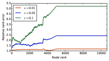
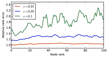
Figure 3: Relative rank error on PGPgiantcompo for nodes ordered by rank. On the left, relative errors of all nodes. On the right, relative errors of the 100 nodes with highest betweenness.

5.3 Running times

In this section, we discuss the running times of all the algorithms, the speedups of the exact incremental approaches (GMB, KDB and NPR) on BA and the speedups of our algorithm on RK. In all of our tests on unweighted graphs, KDB performs worse than GMB, therefore we only report the results of GMB. Figure 4 shows the behavior of the four algorithms for unweighted graphs on PGPgiantcompo. Since GMB can only process edges one by one, its running time increases linearly with the batch size, becoming slower than the static algorithm already with a batch size of 64. Our algorithm shows much better speedups and proves to be significantly faster than recomputation even with a batch of size 1024. The reasons for our high speedup are mainly two: First, we process the updates in a batch, processing only once the nodes affected by multiple edge insertions. Secondly, our algorithm does not need to recompute the dependencies, in contrast to all dynamic algorithms based on BA (i. e. all existing dynamic exact algorithms). For each SSSP, the dependencies need to be recomputed not only for nodes whose distance or number of shortest paths from the source has changed after the edge insertion(s), but also for all the intermediate nodes in the old shortest paths, even if their distance and number of shortest paths are not affected. This number is significantly higher, since for every node which changes its distance or increases its number of shortest paths, the dependencies of all the nodes in all the old shortest paths are affected.

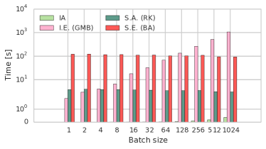
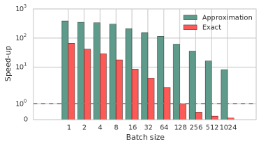
(a) Running times and speedups on Dorogovtsev-Mendes synthetic graphs ($m=40k$), with $\epsilon=0.05$ with batches of different sizes. Left: running times of the four algorithms: static exact (BA), static approximation (RK), incremental exact (GMB) and IA. Right: comparison of the speedups of GMB on BA and of IA on RK.

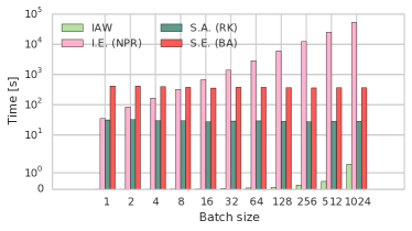
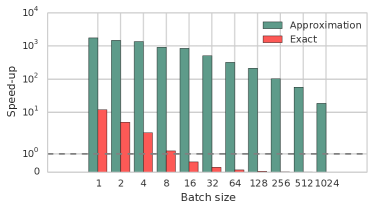
(b) Running times and speedups on weighted synthetic graphs ($m=40k$), with $\epsilon=0.05$ with batches of different sizes. Left: running times of the four algorithms: static exact (BA), static approximation (RK), incremental exact (NPR) and IAW. Right: comparison of the speedups of NPR on BA and of IAW on RK.

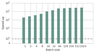
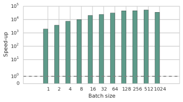
(c) Left: speedups of IA on GMB on unweighted synthetic graphs ($m=40k$). Right: speedups of IAW on NPR on weighted synthetic graphs. IA and IAW run with $\epsilon=0.05$.

Figure 6: Additional experimental results

Results on synthetic unweighted graphs are analogous to those shown in Figure 4 and can be found in the Appendix (Figure 6(a) in Section 0.C). We did the same comparison on synthetic weighted graphs (described in Section 5.1), using NPR instead of GMB. We observed that, even though NPR is theoretically faster than recomputing from scratch, its speedups are very small (see Figure 6(b) in Section 0.C). Figure 6(c) in Section 0.C shows the speedups of IAW on NPR and IA on GMB. Both NPR and GMB have very high memory requirements ($O(n^{2}+mn)$), which makes the algorithms unusable on networks with more than a few thousand edges. The memory requirement is the same also for all other existing dynamic algorithms, with the exception of KDB, which requires $O(n^{2})$ memory, impractical for large networks. Since the exact algorithms are not scalable, for the comparison on larger networks we used only RK and our algorithms. Figure 5 (left) shows the speedups of our algorithm IA on coPapersCiteseer. In this case, the average running time for RK is always approximatively 420 seconds, while for IA it ranges from 0.02 seconds (for a single edge update) to 6.2 seconds (for a batch of 1024 edges). Figure 5 (right) summarises the speedups obtained in the networks of Table 1. The red dots represent the average speedup among the networks for a particular batch size and the shaded areas represent the interval where the different speedups lie. The average speedup is between $10^{3}$ and $10^{4}$ for a single-edge update and between $10$ and $10^{2}$ for a batch size of 1024. Even for graphs with the worst speedups (basically the smallest ones), a batch of this dimension can always be processed faster than recomputation.

Graph	Time RK [s]	Time IA [s] ($b=1$)	Time IA [s] ($b=1024$)	Speedup ($b=1$)	Speedup ($b=1024$)
PGPgiantcompo	3.894	0.009	1.482	432.6	2.6
as-22july06	3.437	0.020	0.520	171.8	6.6
caidaRouterLevel	64.781	0.023	2.193	2816.5	29.5
email-Enron	82.568	0.016	0.750	5160.5	110.0
coAuthorsCiteseer	65.474	0.009	1.008	7274.8	64.9
coAuthorsDBLP	109.939	0.009	1.201	12215.4	91.5
citationCiteseer	192.609	0.030	4.229	6420.3	45.5
belgium.osm	666.144	1.049	48.370	635.0	13.7
Texas84.facebook	344.075	0.147	21.829	2340.6	15.7
netherlands.osm	878.148	1.292	31.802	679.6	27.6
coPapersCiteseer	427.142	0.025	6.186	17085.6	69.0
coPapersDBLP	497.617	0.009	3.027	55290.7	164.3

Table 2: Average running times and speedups on real graphs for batch size $b$. All the algorithms were run with $\epsilon=0.05$ and $\delta=0.1$ and averaged over 10 runs.

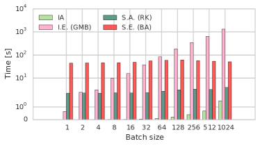
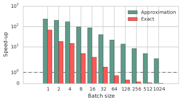
Figure 4: Running times and speedups on PGPgiantcompo, with $\epsilon=0.05$ and with batches of different sizes. On the left, running times of the four algorithms: static exact (BA), static approximation (RK), incremental exact (GMB) and our incremental approximation IA. On the right, comparison of the speedups of GMB on BA and of IA on RK.

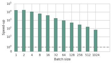
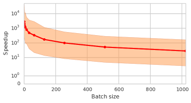
Figure 5: On the left, speedups of IA on RK on the coPapersCiteseer network, run with $\epsilon=0.05$. On the right, geometric mean of speedups over all real networks.

6 Conclusions

Because betweenness centrality considers all shortest paths between pairs of nodes, its exact computation is out of reach for the large complex networks that come up in many applications today. However, approximate scores obtained by sampling paths are often sufficient to identify the most important nodes and rank nodes in an order that is very similar to exact BC. Since many applications are concerned with rapidly evolving networks, we have explored whether a dynamic approach – which updates paths when a batch of new edges arrives – is more efficient than recomputing BC scores from scratch. Our conclusions are drawn from experiments on a diverse set of real-world networks with simulated dynamics. We introduce two dynamic betweenness approximation algorithms, for weighted and unweighted graphs respectively. Their common method is based on the static RK approximation algorithm and inherits its provable bound on the maximum error. Through reimplementation and experiments, we show that previously proposed dynamic BC algorithms scale badly, especially due to an $O(n^{2})$ memory footprint. Combining a dynamic approach with approximation, our method is more scalable and is the first dynamic one applicable to networks with millions of edges (without using external memory).

As an intermediate result of independent interest, we also propose an asymptotically faster algorithm for updating a solution to the SSSP problem in unweighted graphs. The dynamic updating of paths implies a higher memory footprint, but also enables significant speedups compared to recomputation (e. g. factor 100 for a batch of 1024 edge insertions). The scalability of our algorithms is primarily limited by the available memory. Each sampled path requires $O(n)$ memory and the number of required samples grows quadratically as the error bound $\epsilon$ is tightened. This leaves the user with a tradeoff between running time and memory consumption on the one hand and BC score error on the other hand. However, our experiments indicate that even a relatively high error bound (e. g. $\epsilon=0.1$) for the BC scores preserves the ranking for the more important nodes well.

We studied sequential implementations for simplicity and comparability with related work, but parallelization is possible and can yield further speedups in practice. Our implementations are based on NetworKit, the open-source framework for high-performance network analysis, and we plan to publish our source code in upcoming releases of the package.

Acknowledgements.

This work is partially supported by German Research Foundation (DFG) grant FINCA (Fast Inexact Combinatorial and Algebraic Solvers for Massive Networks) within the Priority Programme 1736 Algorithms for Big Data and project Parallel Analysis of Dynamic Networks – Algorithm Engineering of Efficient Combinatorial and Numerical Methods, which is funded by the Ministry of Science, Research and the Arts Baden-Württemberg. We thank Pratistha Bhattarai (Smith College) for help with the experimental evaluation. We also thank numerous contributors to the NetworKit project.

Appendix 0.A Proof of Lemma 2

Proof

To see that $p^{\prime}_{st}$ is a shortest path of $G^{\prime}$, it is sufficient to notice that, if $d^{\prime}_{s}(t)=d_{s}(t)$ and $\sigma^{\prime}_{s}(t)=\sigma_{s}(t)$, then all the shortest paths between $s$ and $t$ in $G$ are shortest paths also in $G^{\prime}$.

Let $p^{\prime}_{xy}$ be a shortest path of $G^{\prime}$ between nodes $x$ and $y$. Basically, there are two possibilities for $p^{\prime}_{xy}$ to be the $k$-th sample. Naming $e_{1}$ the event $\{\mathcal{S}_{xy}=\mathcal{S}^{\prime}_{xy}\}$ (the set of shortest paths between $x$ and $y$ does not change after the edge insertion) and $e_{2}$ the complementary event of $e_{1}$, we can write $\Pr(p^{\prime}_{(k)}=p^{\prime}_{xy})$ as $\Pr(p^{\prime}_{(k)}=p^{\prime}_{xy}\cap e_{1})+\Pr(p^{\prime}_{(k)}=p^{\prime}_{xy}\cap e_{2})$.

Using conditional probability, the first addend can be rewritten as $\Pr(p^{\prime}_{(k)}=p^{\prime}_{xy}\cap e_{1})=\Pr(p^{\prime}_{(k)}=p^{\prime}_{xy}|e_{1})\Pr(e_{1})$. As the procedure $\mathcal{P}$ keeps the old shortest path when $e_{1}$ occurs, then $\Pr(p^{\prime}_{(k)}=p^{\prime}_{xy}|e_{1})=\Pr(p_{(k)}=p^{\prime}_{xy}|e_{1})=\frac{1}{n(n-1)}\frac{1}{\sigma_{x}(y)}$, which is also equal to $\frac{1}{n(n-1)}\frac{1}{\sigma^{\prime}_{x}(y)}$, since $\sigma_{x}(y)=\sigma^{\prime}_{x}(y)$ when we condition on $e_{1}$. Therefore, $\Pr(p^{\prime}_{(k)}=p^{\prime}_{xy}\cap e_{1})=\frac{1}{n(n-1)}\frac{1}{\sigma^{\prime}_{x}(y)}\cdot\Pr(e_{1})$.

Analogously, $\Pr(p^{\prime}_{(k)}=p^{\prime}_{xy}\cap e_{2})=\Pr(p^{\prime}_{(k)}=p^{\prime}_{xy}|e_{2})\Pr(e_{2})$. In this case, $\Pr(p^{\prime}_{(k)}=p^{\prime}_{xy}|e_{2})=\frac{1}{n(n-1)}\cdot\frac{1}{\sigma^{\prime}_{x}(y)}$, since this is the probability of the node pair $(x,y)$ to be the $k$-th sample in the initial sampling and of $p^{\prime}_{xy}$ to be selected among other paths in $\mathcal{S}^{\prime}_{xy}$. Then, $\Pr(p^{\prime}_{(k)}=p^{\prime}_{xy}\cap e_{2})=\frac{1}{n(n-1)}\cdot\frac{1}{\sigma^{\prime}_{x}(y)}\cdot\Pr(e_{2})=\frac{1}{n(n-1)}\cdot\frac{1}{\sigma^{\prime}_{x}(y)}\cdot(1-\Pr(e_{1}))$. The probability $\Pr(p^{\prime}_{(k)}=p^{\prime}_{xy})$ can therefore be rewritten as

$$\Pr(p^{\prime}_{(k)}=p^{\prime}_{xy})=\mbox{$\frac{1}{n(n-1)}\frac{1}{\sigma^{\prime}_{x}(y)}\cdot\Pr$($e_{1}$)+$\frac{1}{n(n-1)}\frac{1}{\sigma^{\prime}_{x}(y)}\cdot$(1-$\Pr$($e_{1}$))}=\frac{1}{n(n-1)}\frac{1}{\sigma^{\prime}_{x}(y)}.$$

∎

Appendix 0.B Pseudocode of RK, UpdateSSSP and UpdateSSSPW.

Input : Graph $G=(V,E),\epsilon,\delta\in(0,1)$

Output : A set of approximations of the betweenness centrality of the nodes in $V$

1 foreach node $v\in V$ do

2       $\tilde{c}_{B}$ $(v)\leftarrow 0$;

3      

4 end foreach

5VD ($G$)$\leftarrow$getVertexDiameter($G$);

6 $r\leftarrow(c/\epsilon^{2})(\lfloor\log_{2}(\textnormal{{VD}}(G)-2)\rfloor+\ln(1/\delta))$;

7 for $i\leftarrow 1$ to $r$ do

8       $(s_{i},t_{i})\leftarrow$ sampleUniformNodePair($V$);

9       $(d_{s_{i}},\sigma_{s_{i}},P_{s_{i}})\leftarrow$ computeExtendedSSSP($G,s_{i}$);

       // Now one path from $s_{i}$ to $t_{i}$ is sampled uniformly at random

10       $v\leftarrow t_{i}$;

11       $p_{(i)}\leftarrow$ empty list;

12       while $P_{s_{i}}(v)\neq\{s_{i}\}$ do

13             sample $z\in P_{s_{i}}(v)$ with $\Pr=\sigma_{s_{i}}(z)/\sigma_{s_{i}}(v)$;

14             $\textnormal{{$\tilde{c}_{B}$}}(z)\leftarrow\textnormal{{$\tilde{c}_{B}$}}(z)+1/r$;

15             add $z\rightarrow p_{(i)}$; $v\leftarrow z$;

16            

17       end while

18      

19 end for

20return $\{(v,\textnormal{{$\tilde{c}_{B}$}}(v)),\>v\in V\}$

Algorithm 2 Computation of the approximated betweenness centralities on the initial graph $G$ (RK algorithm)

Input : Graph $G=(V,E)$, source node $s$, old values of $d_{s}$, $\sigma_{s}$ and $P_{s}$, batch of edge insertion $\beta={e_{1},...,e_{k}}$

Output : Updated values of $d_{s}$, $\sigma_{s}$ and $P_{s}$

1 $Q\leftarrow$ empty min-based priority queue;

2 foreach $e=\{u,v\}\in\beta$ do

3       insert $e$ into $E$;

4       if $d_{s}(v)\geq d_{s}(u)+\mathsf{w}(e)$ then

5             insert $v$ in $Q$ with $p_{Q}(v)=d_{s}(u)+\mathsf{w}(e)$ or, if already in $Q$ and $p_{Q}(v)>d_{s}(u)+\mathsf{w}(e)$, set $p_{Q}(v)\leftarrow d_{s}(u)+\mathsf{w}(e)$;

6       end if

7      if $d_{s}(u)\geq d_{s}(v)+\mathsf{w}(e)$ then

8             insert $u$ in $Q$ with $p_{Q}(u)=d_{s}(v)+\mathsf{w}(e)$ or, if already in $Q$ and $p_{Q}(u)>d_{s}(v)+\mathsf{w}(e)$, set $p_{Q}(u)\leftarrow d_{s}(v)+\mathsf{w}(e)$;

9       end if

10      

11 end foreach

12 while $Q\neq\emptyset$ do

13       $(w,p)\leftarrow$ extractMin ($Q$);

14       $d_{s}(w)\leftarrow p$; $P_{s}(w)\leftarrow\emptyset$; $\sigma_{s}(w)\leftarrow 0$;

15       foreach incident edge $\{z,w\}$ do

16             if $d_{s}(w)=d_{s}(z)+\mathsf{w}(\{z,w\})$ then

17                   add $z$ to $P_{s}(w)$;

18                   $\sigma_{s}(w)\leftarrow\sigma_{s}(w)+\sigma_{s}(z)$;

19                  

20             end if

21            if $d_{s}(z)\geq d_{s}(w)+\mathsf{w}(\{w,z\})$ then

22                   insert $z$ in $Q$ with $p_{Q}(z)=d_{s}(w)+\mathsf{w}(\{z,w\})$ or, if already in $Q$ and $p_{Q}(z)>d_{s}(w)+\mathsf{w}(\{z,w\})$, set $p_{Q}(z)\leftarrow d_{s}(w)+\mathsf{w}(\{z,w\})$;

23             end if

24            

25       end foreach

26      

27 end while

return $(d_{s},\sigma_{s},P_{s})$

Algorithm 3 UpdateSSSPW

Input : Graph $G=(V,E)$, source node $s$, old values of $d_{s}$, $\sigma_{s}$ and $P_{s}$, batch of edge insertion $\beta={e_{1},...,e_{k}}$, maximum distance $d_{max}$

Output : Updated values of $d_{s}$, $\sigma_{s}$ and $P_{s}$

Assume : $color[v]=white$ for all $v\in V$

1 $Q[]\leftarrow$ array of empty queues of size $d_{max}$;

2 foreach $e=\{u,v\}\in\beta$ do

3       insert $e$ into $E$;

4       if $d_{s}(u)<d_{s}(v)$ then

5             $k\leftarrow d_{s}(u)+1$; enqueue $v\rightarrow Q[k]$;

6            

7       end if

8      if $d_{s}(v)<d_{s}(u)$ then

9             $k\leftarrow d_{s}(v)+1$; enqueue $u\rightarrow Q[k]$;

10            

11       end if

12      

13 end foreach

14 $k\leftarrow 1$;

15 while $k<d_{max}$ do

16       while $Q[k]\neq\emptyset$ do

17             dequeue $w\leftarrow Q[k]$;

18             if color$(w)=$black then

19                   continue;

20                  

21             end if

22            $color(w)\leftarrow black$; $d_{s}(w)\leftarrow k$; $P_{s}(w)\leftarrow\emptyset$; $\sigma_{s}(w)\leftarrow 0$;

23             foreach incident edge $(z,w)$ do

24                   if $d_{s}(w)=d_{s}(z)+1$ then

25                         add $z$ to $P_{s}(w)$; $\sigma_{s}(w)\leftarrow\sigma_{s}(w)+\sigma_{s}(z)$;

26                        

27                   end if

28                   if color$[z]=$white and $d_{s}(z)\geq d_{s}(w)+1$ then

29                         $color[z]\leftarrow gray$; enqueue $z\rightarrow Q[k+1]$;

30                        

31                   end if

32                  

33             end foreach

34            

35       end while

36      $k\leftarrow k+1$;

37      

38 end while

39 Set to white all the nodes that have been in $Q$;

return $(d_{s},\sigma_{s},P_{s})$

Algorithm 4 UpdateSSSP

Appendix 0.C Additional experimental results

References

- [1] David A. Bader, Shiva Kintali, Kamesh Madduri, and Milena Mihail. Approximating betweenness centrality. In Anthony Bonato and Fan R. K. Chung, editors, Workshop on Algorithms and Models for the Web Graph, volume 4863 of Lecture Notes in Computer Science, pages 124–137. Springer, 2007.
- [2] David A. Bader, Henning Meyerhenke, Peter Sanders, and Dorothea Wagner, editors. Graph Partitioning and Graph Clustering – 10th DIMACS Impl. Challenge, volume 588 of Contemporary Mathematics. AMS, 2013.
- [3] Reinhard Bauer and Dorothea Wagner. Batch dynamic single-source shortest-path algorithms: An experimental study. In 8th International Symposium on Experimental Algorithms (SEA ’09), volume 5526 of LNCS, pages 51–62. Springer, 2009.
- [4] Ulrik Brandes. A faster algorithm for betweenness centrality. Journal of Mathematical Sociology, 25:163–177, 2001.
- [5] Ulrik Brandes and Christian Pich. Centrality estimation in large networks. I. J. Bifurcation and Chaos, 17(7):2303–2318, 2007.
- [6] Annalisa D’Andrea, Mattia D’Emidio, Daniele Frigioni, Stefano Leucci, and Guido Proietti. Dynamically maintaining shortest path trees under batches of updates. In Thomas Moscibroda and Adele A. Rescigno, editors, 20th International Colloquium on Structural Information and Communication Complexity (SIROCCO ’13), volume 8179 of Lecture Notes in Computer Science, pages 286–297. Springer, 2013.
- [7] Annalisa D’Andrea, Mattia D’Emidio, Daniele Frigioni, Stefano Leucci, and Guido Proietti. Experimental evaluation of dynamic shortest path tree algorithms on homogeneous batches. In 13th International Symposium on Experimental Algorithms (SEA ’14), volume 8504 of LNCS, pages 283–294. Springer, 2014.
- [8] Sergei N Dorogovtsev and José FF Mendes. Evolution of networks: From biological nets to the Internet and WWW. Oxford University Press, 2003.
- [9] Linton C. Freeman. A set of measures of centrality based on betweenness. Sociometry, 40(1):35–41, March 1977.
- [10] Daniele Frigioni, Mario Ioffreda, Umberto Nanni, and Giulio Pasqualone. Experimental analysis of dynamic algorithms for the single source shortest path problem. ACM Jounal of Experimental Algorithmics, 3:5, 1997.
- [11] Daniele Frigioni, Alberto Marchetti-spaccamela, and Umberto Nanni. Fully dynamic output bounded single source shortest path problem (extended abstract). In 7th ACM-SIAM Symposium on Discrete Algorithms (SODA ’96), pages 212–221, 1996.
- [12] Daniele Frigioni, Alberto Marchetti-spaccamela, and Umberto Nanni. Semi-dynamic algorithms for maintaining single-source shortest path trees. Algorithmica, 22:250–274, 2008.
- [13] Robert Geisberger, Peter Sanders, and Dominik Schultes. Better approximation of betweenness centrality. In J. Ian Munro and Dorothea Wagner, editors, 10th Workshop on Algorithm Engineering and Experiments (ALENEX ’08), pages 90–100. SIAM, 2008.
- [14] Oded Green, Robert McColl, and David A. Bader. A fast algorithm for streaming betweenness centrality. In SocialCom/PASSAT, pages 11–20. IEEE, 2012.
- [15] Min joong Lee, Ryan H. Choi, Jungmin Lee, Chin wan Chung, and Jaimie Y. Park. Qube: a quick algorithm for updating betweenness centrality, 2012.
- [16] Miray Kas, Matthew Wachs, Kathleen M. Carley, and L. Richard Carley. Incremental algorithm for updating betweenness centrality in dynamically growing networks. In Advances in Social Networks Analysis and Mining 2013 (ASONAM ’13), pages 33–40. ACM, 2013.
- [17] Nicolas Kourtellis, Gianmarco De Francisci Morales, and Francesco Bonchi. Scalable online betweenness centrality in evolving graphs. CoRR, abs/1401.6981, 2014.
- [18] Meghana Nasre, Matteo Pontecorvi, and Vijaya Ramachandran. Betweenness centrality - incremental and faster. CoRR, abs/1311.2147, 2013.
- [19] G. Ramalingam and Thomas Reps. An incremental algorithm for a generalization of the shortest-path problem. Journal of Algorithms, 21:267–305, 1992.
- [20] G. Ramalingam and Thomas Reps. On the computational complexity of dynamic graph problems. THEORETICAL COMPUTER SCIENCE, 158:233–277, 1996.
- [21] Matteo Riondato and Evgenios M. Kornaropoulos. Fast approximation of betweenness centrality through sampling. In 7th ACM International Conference on Web Search and Data Mining (WSDM ’14), pages 413–422. ACM, 2014.
- [22] Liam Roditty and Uri Zwick. On dynamic shortest paths problems. Algorithmica, 61(2):389–401, 2011.
- [23] Christian Staudt, Aleksejs Sazonovs, and Henning Meyerhenke. Networkit: An interactive tool suite for high-performance network analysis. http://arxiv.org/abs/1403.3005, 2014.