The one-dimensional thermal properties for the relativistic harmonic oscillators

Abstract

In this paper, we want to improved the calculations of the thermodynamic quantities of the relativistic Harmonic oscillator using the Hurwitz zeta function. The comparison of our results with those obtained by a method based on the Euler-MacLaurin approach has been made.

I Introduction

The relativistic harmonic oscillator is one of the most important quantum system, as it is one of the very few that can be solved exactly.

The Dirac relativistic oscillator (DO) interaction is an important potential both for theory and application. It was for the first time studied by Ito et al 1 (1). They considered a Dirac equation in which the momentum $\vec{p}$ is replaced by $\vec{p}-im\beta\omega\vec{r}$, with $\vec{r}$ being the position vector, $m$ the mass of particle, and $\omega$ the frequency of the oscillator. The interest in the problem was revived by Moshinsky and Szczepaniak 2 (2), who gave it the name of Dirac oscillator (DO) because, in the non-relativistic limit, it becomes a harmonic oscillator with a very strong spin-orbit coupling term. Physically, it can be shown that the (DO) interaction is a physical system, which can be interpreted as the interaction of the anomalous magnetic moment with a linear electric field 3 (3, 4). The electromagnetic potential associated with the DO has been found by Benitez et al5 (5). The Dirac oscillator has attracted a lot of interest both because it provides one of the examples of the Dirac’s equation exact solvability and because of its numerous physical applications 6 (6, 7, 8, 9). Fortunately Franco-Villafane et al 10 (10), in order to vibrate this oscillator, exposed the proposal of the first experimental microwave realization of the one-dimensional (DO).

The thermal properties of the one-dimensional Dirac equation in a Dirac oscillator interaction was at first considered by Pacheco et al 11 (11) . The authors have been calculated the all thermal quantities of the oscillator by using the Euler-MacLaurin formula. Although this method allows to obtain the all thermal properties of the system, the expansion of the partition function using it could be valid only for higher temperatures regime, but not otherwise. Also, the partition function at $T=0\mbox{K}$ reveals a total divergence (see Annexe A). Encouraged by the experimental realization of a Dirac oscillator, we are interested in: (i) to improve the calculations of the thermodynamics properties for the relativistic harmonic oscillators in all range of temperatures, and (ii) to remove the divergence appears in the partition function at $T=0\mbox{K}$. Both objectives can be achieved by using a method based on the zeta function 12 (12, 13). This method has been used by 14 (14) with the aim of calculating the partition function in the case of the graphene. We note here that the zeta function has been applied successfully in different areas of physics, and the examples vary from ordinary quantum and statistical mechanics to quantum field theory (see for example 15 (15)).

Thus, the main goal of this paper is the improvement of the calculations of all thermal quantities of the one-dimensional Dirac oscillator. This work is organized as follows: In section. 2, we review the solutions of both Dirac and Klein-Gordon oscillators in one dimension. Section. 3 is devoted to our numerical results and discussions. Finally, Section. 4 will be a conclusion.

II Review of the solutions of both Dirac and Klein-Gordon oscillators in one dimension

II.1 one-dimensional Klein-Gordon oscillator

The free Klein-Gordon oscillator is written by

$$\left(p_{x}^{2}-\frac{E^{2}-m_{0}^{2}c^{4}}{c^{2}}\right)\phi=0.$$ (1)

In the presence of the interaction of the type of Dirac oscillator, it becomes

$$\left[c^{2}\left(p_{x}+im_{0}\omega x\right)\cdot\left(p_{x}-im_{0}\omega x\right)-E^{2}+m_{0}^{2}\right]\phi\left(x\right)=0,$$ (2)

or

$$\left(\frac{p_{x}^{2}}{2m_{0}}+\frac{m_{0}\omega{}^{2}}{2}x^{2}\right)\phi\left(x\right)=\left(\frac{m_{0}c^{2}\hbar\omega+E^{2}-m_{0}^{2}c^{4}}{2m_{0}c^{2}}\right)\phi\left(x\right)\equiv\tilde{E}\phi\left(x\right),$$ (3)

with

$$\tilde{E}=\frac{m_{0}c^{2}\hbar\omega+E^{2}-m_{0}^{2}c^{4}}{2m_{0}c^{2}}.$$ (4)

The equation (3) is the standard equation of a harmonic oscillator in $1D$. The energy levels are well known, and the solutions are

$$\epsilon_{n}=\pm m_{0}c^{2}\sqrt{1+2rn}$$ (5)

with $r=\frac{\hbar\omega}{m_{0}c^{2}}$ being a parameter which controls the non relativistic limit.

The eigenfunctions may be expressed in terms of Hermite Polynomial of Degree $n$ as

$$\phi\left(x\right)=\mbox{N}_{\mbox{norm}}\left(\frac{m_{0}\omega}{\pi\hbar}\right)^{\frac{1}{4}}H\left(\sqrt{\frac{m_{0}\omega}{\hbar}}x\right)e^{-\frac{m\omega}{2\hbar}x^{2}}.$$ (6)

where the functions $H$ is the so called Hermite polynomials, and $\mbox{N}_{\mbox{norm}}$ is a normalizing factor 16 (16).

II.2 one-dimensional Dirac oscillator

The one-dimensional Dirac oscillator is

$$\left\{c\cdot\alpha_{x}\cdot\left(p_{x}-im\omega\beta\cdot x\right)+\beta mc^{2}\right\}\psi_{D}=E\psi_{D},$$ (7)

with $\psi_{D}=\left(\begin{array}[]{cc}\psi_{1}&\psi_{2}\end{array}\right)^{T}$, $\alpha_{x}=\sigma_{x}$ and $\beta=\sigma_{z}$.

From Eq. (7), we get a set of coupled equations as follows:

$$\left(E-mc^{2}\right)\psi_{1}=c\left(p_{x}+im\omega x\right)\psi_{2},$$ (8)

$$\left(E+mc^{2}\right)\psi_{2}=c\left(p_{x}-im\omega x\right)\psi_{1}.$$ (9)

Using Eq. (9), we have

$$\psi_{2}\left(x\right)=\frac{c\left(p_{x}-im\omega x\right)}{E+mc^{2}}\psi_{1}\left(x\right).$$ (10)

Putting Eq. (10) into (8), we get

$$\left[c^{2}\left(p_{x}+im\omega x\right)\left(p_{x}-im\omega x\right)-E^{2}+m^{2}\right]\psi_{1}\left(x\right)=0,$$ (11)

or

$$\left(\frac{p_{x}^{2}}{2m}+\frac{m\omega^{2}}{2}x^{2}\right)\psi_{1}\left(x\right)=\left(\frac{\hbar\omega mc^{2}+E^{2}-m^{2}c^{4}}{2mc^{2}}\right)\psi_{1}\left(x\right)\equiv\tilde{E}\psi_{1}.$$ (12)

The equation (12) is the standard equation of a harmonic oscillator in $1D$. The energy levels are well-known, and are given by

$$\varepsilon_{n}=\pm mc^{2}\sqrt{1+2\bar{r}n}$$ (13)

with $\bar{r}=\frac{\hbar\omega}{mc^{2}}$ is a parameter which controls the non relativistic limit. The eigenfunctions may be expressed in terms of Hermite Polynomial of Degree $n$ a

$$\psi_{1}\left(x\right)=\mbox{N}_{\mbox{norm}}^{{}^{\prime}}\left(\frac{m\omega}{\pi\hbar}\right)^{\frac{1}{4}}H\left(\sqrt{\frac{m\omega}{\hbar}}x\right)e^{-\frac{m\omega}{2\hbar}x^{2}}.$$ (14)

with $\mbox{N}_{\mbox{norm}}^{{}^{\prime}}$ is a normalizing factor. The total associated wave function is

$$\psi_{D}\left(x\right)=\mbox{N}_{\mbox{norm}}^{{}^{\prime}}\left[\begin{array}[]{c}1\\ \frac{c\left(p_{x}-im\omega x\right)}{E+mc^{2}}\end{array}\right]H\left(\sqrt{\frac{m\omega}{\hbar}}x\right)e^{-\frac{m\omega}{2\hbar}x^{2}}.$$ (15)

III Thermal properties of the relativistic harmonic oscillator

Before we study the thermodynamic properties of both oscillators, we can see that the form of the spectrum of energy (see Eqs. (5) and (13)), for both cases, is the same. As consequently, the numerical thermal quantities found, for both oscillators, are similar . Thus, we focus, firstly, on the study of the thermal properties of a Dirac oscillator, and then all results obtained can be extended to the case of the one-dimensional Klein-Gordon oscillator.

III.1 Methods

In order to obtain all thermodynamic quantities of the relativistic harmonic oscillator, we concentrate, at first, on the calculation of the partition function $Z$. The last is defined by

$$Z=\sum_{n}e^{-\beta E_{n}}=\sum_{n}e^{-\frac{\sqrt{1+2rn}}{\tau}}$$ (16)

With the following substitutions:

$$\alpha=\frac{1}{2r},\leavevmode\nobreak\ \gamma=\sqrt{2r},$$ (17)

it becomes

$$Z=\sum_{n}e^{-\frac{\gamma}{\tau}\sqrt{\alpha+n}},$$ (18)

with $\tau=\frac{k_{B}T}{mc^{2}}$ denotes the reduce temperature.

Using the formula 12 (12, 13)

$$e^{-x}=\frac{1}{2\pi i}\int_{C}dsx^{-s}\Gamma\left(s\right),$$ (19)

the sum in Eq. (18) is transformed into

$$\sum_{n}e^{-\frac{\gamma}{\tau}\sqrt{\alpha+n}}=\frac{1}{2\pi i}\int_{C}ds\left(\frac{\gamma}{\tau}\right)^{-s}\sum_{n}\left(n+\alpha\right)^{-\frac{s}{2}}\Gamma\left(s\right)=\frac{1}{2\pi i}\int_{C}ds\left(\frac{\gamma}{\tau}\right)^{-s}\zeta_{H}\left(\frac{s}{2},\alpha\right)\Gamma\left(s\right),$$ (20)

with $x=\frac{\gamma}{\tau}\sqrt{\alpha+n}$, and $\Gamma\left(s\right)$ and $\zeta_{H}\left(\frac{s}{2},\alpha\right)$ are respectively the Euler and Hurwitz zeta function. Applying the residues theorem, for the two poles $s=0$ and $s=2$, the desired partition function is written down in terms of the Hurwitz zeta function as follows:

$$Z\left(\tau\right)=\frac{\tau^{2}}{2r}+\zeta_{H}\left(0,\alpha\right).$$ (21)

Now, using that

$$\zeta_{H}\left(0,\alpha\right)=\frac{1}{2}-\alpha,$$ (22)

the final partition function is transformed into

$$Z\left(\tau\right)=\frac{\tau^{2}}{2r}+\frac{1}{2}-\frac{1}{2r}.$$ (23)

From this definition, all thermal properties of both fermionic and bosonic oscillators can be obtained.

III.2 Numerical results and discussions

Fig. 1 depicted the one-dimensional thermal properties of both Dirac and Klein-Gordon oscillators. Following the figure, all thermal quantities are plotted versus a reduced temperature $\tau$: here we have taken $r=1$ which corresponds to the relativistic region . From the curve of the numerical entropy function, no abrupt change, around $\tau_{0}$, has been identified. This means that the curvature, observed in the specific heat curve, does not exhibit or indicate an existence of a phase transition around a $\tau_{0}$ temperature.

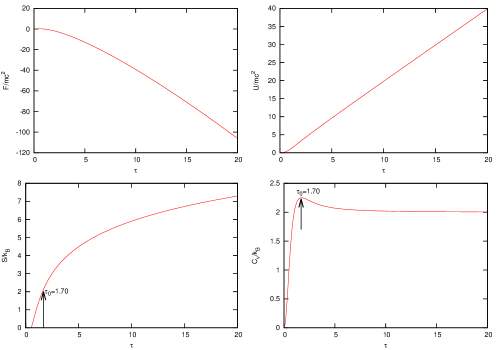
Figure 1: One-dimensional thermal properties for both oscillators in the case where $r=1$.

Now, according to the condition on $\alpha$ parameter which appears in the zeta function (see Annexe B), we can distinguish two regions: the first, defined by $r\geq 0.5$, corresponds to the relativistic regime, and the other, with $r<0.5$, represents the non-relativistic regime. These observations, for both Dirac and Klein-Gordon oscillators, are shown clearly in the Fig. 2. Also, following the same figure, three remarks can be made:

• The $\tau_{0}$ reduce temperature increases for the values of $r>1$, and disappears when $r<1$.

• When $r<0.5$ all curves coincide with the non-relativistic limit ($r=10^{-10}$).

• For all values of $r$ , all curves of the specific heat coincide with the limit $2k_{B}$.

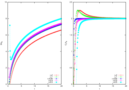
(a) for the values of $r\geq 0.5$

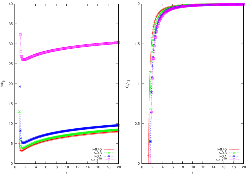
(b) for the values of $r<0.5$

Figure 2: The entropy and specific heat as a function of a reduce temperature $\tau$ for different values of the parameter $r$.

Pacheco et al 11 (11) have been studied the thermal properties of a Dirac oscillator in one dimension. They obtained all thermodynamics quantities by using the Euler-MacLaurin approximation(see Annexe A). The formalism used by 11 (11) is valid, only, for higher temperatures. So, in order to cover all range of temperatures, we have employed the Hurwitz zeta function method.

In the Fig. 3, we are focused on the curves of the numerical specific heat calculated for different values of the parameter $r$. Then, for comparison with 11 (11), we have inserted the numerical calculation of the specific heat based on the Euler-MacLaurin approximation. Thus, we can see that our results can be considered as an improvements of the results obtained in 11 (11). This consideration can be argued as follows: (i) all thermal quantities obtained from the zeta function method are valid in all range of temperatures, and (ii) the divergence of the partition function, which appears in Euler-MacLaurin formula, has been removed. All results obtained in this case can be extended to the case of the Klein-Gordon oscillator (see Fig. 4).

Figure 3: Comparison of our specific heat for different values of $r$ with that obtained by using the Euler-MacLaurin formula for a Dirac oscillator in one-dimension.

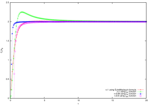
Figure 4: Comparison of our specific heat for different values of $r$ with that obtained by using the Euler-MacLaurin formula for a Klein-Gordon oscillator in one-dimension.

Finally, one may compute the vacuum expectation value of the energy defined by 15 (15)

$$\epsilon_{0}=\lim_{s\rightarrow-1}\sum_{n=0}^{\infty}\left|\epsilon_{n}\right|^{-s}.$$ (24)

From the spectrum of energy of a Dirac oscillator (Eq. (13)), the equation (24) can be expressed in terms of the $\zeta_{H}$ as follows:

$$\frac{\epsilon_{0}}{mc^{2}}=\sqrt{2r}\zeta_{H}\left(-\frac{1}{2},\frac{1}{2r}\right).$$ (25)

Using the asymptotic series corresponding to the Hurwitz zeta function (see Annexe B), Eq. (25) becomes

$$\frac{\epsilon_{0}}{mc^{2}}=-\frac{1}{3r}+\frac{1}{2}-\frac{2}{3}\sum_{k=2}^{\infty}\frac{B_{k}}{k!}\frac{\Gamma\left(-\frac{3}{2}+k\right)}{\Gamma\left(-\frac{3}{2}\right)}\left(\frac{1}{2r}\right)^{1-k}.$$ (26)

In the Fig. (5), we show the $\frac{\epsilon_{0}}{mc^{2}}$ as a function of the parameter $r$. We can see that the vacuum expectation value of the energy, which depend on the parameter $r$, can approximate with

$$\frac{\epsilon_{0}}{mc^{2}}\approxeq-\frac{1}{3r}+\frac{1}{2}.$$ (27)

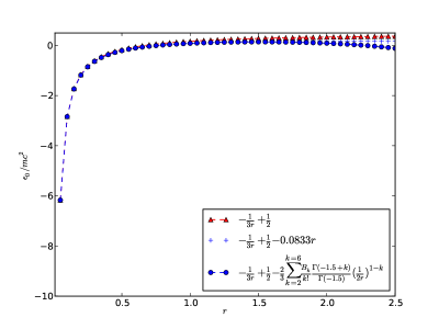
Figure 5: The reduce vacuum expectation value of the energy $\frac{\epsilon_{0}}{mc^{2}}$ versus a parameter $r$ around a relativistic region.

IV Conclusion

In this work, we reviewed the relativistic harmonic oscillator for both fermionic and bosonic massive particles in one dimension. The statistical quantities of both Dirac and Klein-Gordon oscillators were investigated by employing the zeta function method. The both cases have been confronted with those obtained by using the Euler-MacLaurin formula. The vacuum expectation value of the energy, for both oscillators, has been estimated.

Appendix A Euler-MacLaurin formula

The partition function Z of the Dirac oscillator at finite temperature $T$ is obtained through the Boltzmann factor 7 (7),

$$Z=\sum_{n=0}^{n}e^{-\beta\left(E_{n}-E_{0}\right)}=e^{\beta\sqrt{b}}\sum_{n=0}^{n}e^{-\beta\sqrt{an+b}},$$ (28)

where $\beta=\frac{1}{k_{B}T}$ , $k_{B}$ is the Boltzmann constant, $E_{0}$ is the ground state energy correspondent to $n=0$.

Before entering in the calculations, let us test the convergence of the series of (28). For that, we apply the integral test which shows that the series and the integral converge or diverge together. So, from (28), we can see that the function $f(x)$, where

$$f\left(x\right)=e^{-\beta\sqrt{an+b}},$$ (29)

is a decreasing positive function, and the integral

$$\int_{0}^{\infty}f\left(x\right)dx=\frac{2}{a\beta^{2}}e^{-\beta\sqrt{b}}\left(1+\beta\sqrt{b}\right),$$ (30)

is convergent. This means that, according to the criterion of the integral test, the numerical partition function Z converges.

In order to evaluate this function, we use the Euler-MacLaurin formula defined as follows

$$\sum_{x=0}^{\infty}f\left(x\right)=\frac{1}{2}f\left(0\right)+\int_{0}^{\infty}f\left(x\right)dx-\sum_{p=1}^{\infty}\frac{1}{\left(2p\right)!}B_{2p}f^{\left(2p-1\right)}\left(0\right),$$ (31)

Here, $B_{2p}$ are the Bernoulli numbers, $f^{(2p-1)}$ is the derivative of order $\left(2p-2\right)$. In our case, we have taken $B_{2}=\frac{1}{6}$ and $B_{4}=-\frac{1}{30}$.

In our case, we have used

$$f^{\left(1\right)}\left(0\right)=\frac{a\beta}{2\sqrt{b}}e^{-\beta\sqrt{b}}$$ (32)

$$f^{\left(3\right)}\left(0\right)=\left[\frac{-3\beta a^{3}}{8\left(b\right)^{5/2}}-\frac{3\beta^{2}a^{3}}{8\left(b\right)^{2}}-\frac{\beta^{3}a^{3}}{8\left(b\right)^{3/2}}\right]e^{-\beta\sqrt{b}}.$$ (33)

Following Eqs. (31), (32) and (33), the partition function can be cast into

$$Z=\frac{1}{2}+\frac{1}{2r}\tau+\frac{1}{2r}\tau^{2}+\left(\frac{r}{6}-\frac{r^{3}}{60}\right)\frac{1}{\tau}-\frac{1}{30}\frac{r^{3}}{\tau^{2}}-\frac{4}{45}\frac{r^{3}}{\tau^{3}}.$$ (34)

Appendix B Some properties of zeta function

The Riemann zeta function is defined by15 (15)

$$\zeta\left(s\right)=\sum_{n=0}^{\infty}\frac{1}{n^{s}},\leavevmode\nobreak\ \mbox{with}\leavevmode\nobreak\ s\in\mathbb{C}.$$ (35)

Nowadays the Riemann zeta function is just one member of a whole family of zeta function’s (Hurwitz, Epstein,Selberg). The most important of them is the Hurwitz zeta function $\zeta_{H}$ given by

$$\zeta_{H}\left(s,\alpha\right)=\sum_{n=0}^{\infty}\frac{1}{\left(n+\alpha\right)^{s}},$$ (36)

where $0<\alpha\leq 1$, is a well-defined series when $\Re e\left(s\right)>1$, and can be analytically continued to the whole complex plane with one singularity, a simple pole with residue 1 at $s=1$.

An integral representation is

$$\zeta_{H}\left(s,\alpha\right)=\frac{1}{\Gamma\left(s\right)}\int_{0}^{\infty}dtt^{s-1}\frac{e^{-t\alpha}}{1-e^{-t}},\leavevmode\nobreak\ \Re\left(s\right)>1,\leavevmode\nobreak\ \Re\left(\alpha\right)>0.$$ (37)

It can be shown that $\zeta_{H}\left(s,\alpha\right)$ has only one singularity –namely a simple pole at $s=1$ with residue 1 and that it can be analytically continued to the rest of the complex s-plane.

Also, we can shown that $\zeta_{H}\left(s,\alpha\right)$ have the following properties:

$$\zeta_{H}\left(0,\alpha\right)=\frac{1}{2}-\alpha,$$ (38)

$$\zeta_{H}\left(-m,\alpha\right)=-\frac{B_{m+1}\left(\alpha\right)}{m+1},\leavevmode\nobreak\ m\in\mathbb{N},$$ (39)

$B_{r}(a)$ being the Bernoulli polynomials. The asymptotic series corresponding the Hurwitz zeta function is given by

$$\zeta_{H}\left(1+z,\alpha\right)=\frac{1}{z}\alpha^{-z}+\frac{1}{2}\alpha^{-1-z}+\frac{1}{z}\sum_{k=2}^{\infty}\frac{B_{k}}{k!}\frac{\Gamma\left(z+k\right)}{\Gamma\left(z\right)}\alpha^{-z-k},$$ (40)

with $B_{k}$are Bernoulli’s numbers.

References

- (1) D. Itô, K. Mori and E. Carriere, Nuovo Cimento A, 51, 1119 (1967).
- (2) M. Moshinsky and A. Szczepaniak, J. Phys. A: Math. Gen, 22, L817 (1989).
- (3) R. P. Martinez-y-Romero and A. L. Salas-Brito, J. Math. Phys, 33 , 1831 (1992).
- (4) M. Moreno and A. Zentella, J. Phys. A: Math. Gen, 22 , L821 (1989).
- (5) J. Benitez, P. R. Martinez y Romero , H. N. Nunez-Yepez and A. L. Salas-Brito,Phys. Rev. Lett, 64, 1643–5 (1990).
- (6) C. Quesne and V. M. Tkachuk, J. Phys. A: Math. Gen, 41 , 1747–65 (2005).
- (7) A. Boumali and H. Hassanabadi, Eur. Phys. J. Plus. 128, 124 (2013).
- (8) C. Quimbay and P. Strange, arXiv:1311.2021 (2013).
- (9) C. Quimbay and P. Strange, arXiv:1312.5251 (2013).
- (10) A. Franco-Villafane, E. Sadurni, S. Barkhofen, U. Kuhl, F. Mortessagne, and T. H. Selig- man, Phys. Rev. Lett. 111, 170405 (2013).
- (11) M. H. Pacheco, R. R. Landim and C. A. S Almeida, Phys. Lett. A, 311, 93–96 (2003).
- (12) Marina-Aura Dariescu and C. Dariescu, J. Phys.: Condens. Matter 19, 256203 (2007).
- (13) Marina-Aura Dariescu and C. Dariescu, Chaos. Solitons and Fractals 33 , 776–781 (2007).
- (14) Marina-Aura Dariescu and C. Dariescu, Rom. Journ. Phys, 56, 1043–1052, (2011).
- (15) E. Elizalde, Ten physical applications of spectral zeta functions, Springer-Verlag Berlin Heidelberg (1995).
- (16) W. Greiner, Quantum Mechanics: An Introduction, 4th ed, Springer-Verlag, Berlin, (2001).