Extending classical nucleation theory to confined systems

Abstract

Classical nucleation theory has been recently reformulated based on fluctuating hydrodynamics [J.F. Lutsko and M.A. Durán-Olivencia, J. Chem. Phys. 138, 244908(2013)]. The present work extends this effort to the case of nucleation in confined systems such as small pores and vesicles. The finite available mass imposes a maximal supercritical cluster size and prohibits nucleation altogether if the system is too small. We quantity the effect of system size on the nuceation rate. We also discuss the effect of relaxing the capillary-model assumption of zero interfacial width resulting in significant changes in the nucleation barrier and nucleation rate.

I Introduction

Nucleation is a ubiquitous process in nature which has been the subject of extensive research throughout the last century. Nowadays the most well-known understanding of the process relies on Gibbs’ workGibbs (1878a, b); Gibbs et al. (1931) concerning the characterization of phase transformations. Mainly focused on transitions near the equilibrium, Gibbs deduced a simple expression for the work required to form a spherical embryo (so-called cluster) of the new phase within the old one, $W(r)$ with $r$ being the cluster radius. While these efforts set the thermodynamic ground for understanding nucleation phenomena, Volmer and WeberVolmer and Weber (1926); Volmer (1939) were the pioneers to reveal the importance of the kinetics of nucleation. They proposed a rudimentary model to account for the chief characteristics of such phenomenon. A short time later, a more atomistic picture was proposed by Farkas (1927) who developed the idea of Szilard and that was further developed by Becker and Döring (1935) resulting in the equation which now bears their names. Finally, FrenkelFrenkel (1939, 1946) and Zeldovich (1943) reached a similar result which also allows to describe non-steady-state kinetics. Turnbull and Fisher (1949) generalized this formalism in order to describe solid nucleation from a liquid phase, an approach that was readily extended to include nucleation in solids. The nucleation rate expressions derived from all these developments have an Arrhenius-like structureKashchiev (2000); Kelton and Greer (2010) but they differ in the exact expression for the pre-exponential factor. The combination of these ideas comprise a remarkably robust theory which is commonly called Classical Nucleation Theory (CNT).

Besides being a versatile tool, CNT is intuitively appealing and clearly summarizes the basic rules underlying phase transformations. However, while CNT has shown an extraordinary ability to predict the functional dependence of the nucleation rate on the thermodynamic variables involved, it has exhibited a severe disability when it comes to quantitatively explain experimental data. Viisanen et al. (1993); Viisanen and Strey (1994); Hrubý et al. (1996) This flaw has been usually blamed either on a poorly refined expression of the work of cluster formation, or on the heuristic modelling of cluster formation based on macroscopic growth laws, or on the simplicity of the cluster properties assumed by the capillary approach. There has been several attempts to extend and refine CNT, e.g. generalizing the kinetic modelShizgal and Barrett (1989); Kashchiev (1969) to consider wider cluster transitions than that initially assumed by the pioneers of nucleation,Becker and Döring (1935); Kaichew and Stranski (1934); Zeldovich (1943); Frenkel (1939, 1946); Tunitskii (1941) providing more accurate expressions of the free energy barrier by using classical Density Functional TheoryKelton (1991); Lutsko (2011a) (DFT), refining the capillary model,S. Prestipino and Tosatti (2012) or by selecting a different order parameter instead of the cluster size to characterize the nucleation pathway.W. Lechner and Bolhuis (2011) Recently, a new approach to nucleation has been formulatedLutsko (2011b, 2012a, 2012b) based on fluctuating hydrodynamics.Landau and Lifshitz (1959) We will refer to this as Mesoscopic Nucleation Theory (MeNT). This new framework provides a self-consistent justification and extension of more heuristic equilibrium approaches based solely on the free energy. The MeNT provides a general stochastic differential equation (SDE) for the evolution of an arbitrary number of order parameters characterizing the number density field. When the simplest case is considered, that is a single order parameter, a straight-forward connection with CNT is found.Lutsko and Durán-Olivencia (2013) Such a reformulation of CNT, hereafter called dynamical CNT (dCNT), sheds light on the weaknesses of the classical derivation and can be used to construct a more realistic theory in which clusters have finite interfacial width.

The present work aims to continue this development so as to extend dCNT to the case of confined systems. In the last few years there has been a veritable explosion of interest in nucleation due to the development of new techniques, such as microfluidics, that bring us the opportunity to probe the very small and the very fast. Besides, nucleation in confined environments is important for biological processes such as bone formation,Cantaert et al. (2013); Gómez-Morales et al. (2013) in vivo protein crystallization,Bechtel and Bulla (1976); Koopmann et al. (2012) or cavitation in lipid bilayers,Wrenn et al. (2013) to name but a few. However, CNT is based on assumptions that are violated for small systems. For example, when the nucleation of a dense droplet from a weak solution is considered it is assumed that clusters do not consume enough material during nucleation so as to have a noticeable effect on the properties of the mother phase, but this can only be true for large systems. The main goal of this work is therefore to extend dCNT to take into consideration the conservation of mass required for a finite volume with the aim of further developing the classical theory. Following a similar procedure as that presented in a previous work,Lutsko and Durán-Olivencia (2013) a nucleation rate equation is readily obtained. It turns out that the confinement has a strong effect on the energy barrier and, thus, on the nucleation rate. On the one hand, in contrast to infinite systems, the cluster of new phase can only grow to a certain maximal size so that a complete phase transition is not possible. Nevertheless, for sufficiently large and supersaturated systems, this maximal cluster is indeed the stable, equilibrium state. In contrast, if the system is too small, the maximal cluster size is less than the critical radius and no transition takes place. In other words, nucleation is found to be inhibited as a consequence of the size of the container where the experiment is being carried out. On the other hand, nucleation rate is affected for a certain range of volumes when we compare it with the CNT prediction calculated for infinite systems.Lutsko and Durán-Olivencia (2013) Indeed, such a ratio shows a maximum for system sizes close to that which inhibits nucleation. Moreover, considerable corrections arise when a more realistic model for clusters is taken into consideration.

In section II the order-parameter dynamics derived from fluctuating hydrodynamics is modified so that the finite volume limit is taken into account. It is shown that the confinement does not affect the structure of the stochastic differential equation (SDE) derived in Ref. Lutsko, 2012a. The use of this SDE with a modified version of the capillary model that accounts for the finite mass in the system under study is presented in section III.1. In that Section, we give expressions for the attachment rate, the stationary cluster-size distribution, the nucleation rate and the growth rate of super-critical clusters. Section III.2 focuses on the improvement of those results by means of considering clusters with a finite interfacial width. Three models are proposed: in the first the inner density and the interfacial width are the same as in the case of infinite systems, in the second the inner density is chosen so as to minimize the free energy of the stable cluster, and lastly, in the third model, both the interior density and the interfacial width are determined so as to minimize the free energy of the stable cluster. While the first two models yield similar results between them and to the capillary approach, the last one gives rise to large deviations from the other models. These comparisons are presented in section IV. Finally, our results are summarized in section V.

II Theory

The approach we follow in this work, based on Ref. Lutsko, 2012a, requires that a spherical cluster be characterized by its density as a function of distance from its center, $\rho(r;\mathbf{x}(t))$ where $\mathbf{x}$ represents a set of one or more parameters describing the cluster: e.g. its radius, interior density, etc. As indicated, these parameters can change in time according to the following SDE, Lutsko (2011b, 2012a, 2012b) which will be the basis for this study,

$$\frac{dm(r;\mathbf{x}(t))}{dt}= \,D4\pi r^{2}\rho(r;\mathbf{x}(t))\left.\frac{\partial}{\partial r}\frac{\delta\beta F[\rho]}{\delta\rho(\mathbf{r})}\right|_{\rho(r;\mathbf{x}(t))}$$

$$-\sqrt{D8\pi r^{2}\rho(r;\mathbf{x}(t))}\,\xi(r;t),$$ (1)

where $m(r;\mathbf{x}(t))$ stands for the mass inside a spherical shell,

$$m(r;\mathbf{x}(t))=4\pi\int_{0}^{r}\rho(r^{\prime};\mathbf{x}(t))\,r^{\prime 2}dr^{\prime}$$ (2)

and, with $D$ being the diffusion constant, $F[\rho]$ being the Helmholtz free energy, $\beta=1/k_{B}T$ where $k_{B}$ is the Boltzmann constant and $T$ is the absolute temperature, and where $\xi(r;t)$ is a fluctuating force that fulfils

$$\langle\xi(r;t)\xi(r^{\prime};t^{\prime})\rangle=\delta(r-r^{\prime})\delta(t-t^{\prime}).$$ (3)

Note that square brackets in equation (1) have been used to indicate a functional dependence. Finally, it has been shown that equation (1) is Itô-Stratonovich equivalent (see appendix A of Ref. Lutsko, 2012a), for which reason so that either interpretation may be used.

The next step consists of deriving the dynamics of the parameter vector, $\mathbf{x}(t)$, in confined volumes which will open the door to reduced descriptions, specifically to single order-parameter description.

II.1 Order-parameter dynamics in confined systems

The use of a finite number of scalar parameters (so-called order parameters) to describe the density can be a crude simplification but it is also a very useful method to get an approximate representation of the whole problem. Such a reduced description of the real density profile is commonly used in the classical picture, where it is customary to hypothesize that density fluctuations are well characterized by a single order parameter, namely the size of the cluster. While in CNT the order-parameter dynamics is formulated based on heuristic reasoning, MeNT allows us to derive the dynamical equations from a formal point of view, including the case of more than one order parameter. Here, we briefly review the arguments leading to the equations for the order parameter in order to note the effect of imposing a finite volume.

From equation (1) the time-evolution equation governing the order-parameter dynamics is given by,

$$\frac{\partial m(r;\mathbf{x}(t))}{\partial x_{i}}\frac{dx_{i}}{dt}= \,D4\pi r^{2}\rho(r;\mathbf{x}(t))\left.\frac{\partial}{\partial r}\frac{\delta\beta F[\rho]}{\delta\rho(\mathbf{r})}\right|_{\rho(r;\mathbf{x}(t))}$$

$$-\sqrt{D8\pi r^{2}\rho(r;\mathbf{x}(t))}\,\xi(r;t).$$ (4)

Now, let us assume that the container is a sphere of radius $R_{T}$. The line of reasoning presented in section III.B of Ref. (Lutsko, 2012a) remains valid, although we have to take care of imposing the right integration limits in order to consider the confinement. Thus, the latter equation can be transformed into equation (5) multiplying by a function $W_{j}(r;\mathbf{x}(t))$ and integrating up to $R_{T}$,

$$g_{ij}(\mathbf{x})\frac{dx_{i}}{dt}= \,D\int_{0}^{R_{T}}W_{j}(r;\mathbf{x}(t))\rho(r;\mathbf{x}(t))\times$$

$$\times\left(\frac{\partial}{\partial r}\frac{\delta\beta F[\rho]}{\delta\rho(\mathbf{r})}\right)_{\rho(r;\mathbf{x}(t))}4\pi r^{2}dr$$

$$-\int_{0}^{R_{T}}W_{j}(r;\mathbf{x}(t))\sqrt{D8\pi r^{2}\rho(r;\mathbf{x}(t))}\,\xi(r;t)dr,$$ (5)

with

$$g_{ij}(\mathbf{x}(t))=\int_{0}^{R_{T}}W_{j}(r;\mathbf{x}(t))\frac{\partial m(r;\mathbf{x}(t))}{\partial x_{i}}dr$$ (6)

It was shown that if the diffusion matrix $\mathcal{D}_{ij}(\mathbf{x})$ associated to equation (5) and the matrix $g_{ij}(\mathbf{x})$ are assumed proportional, the function $W_{i}$ must be, modulo a multiplicative constant,

$$W_{i}(r;\mathbf{x}(t))=\frac{1}{4\pi r^{2}\rho(r;\mathbf{x}(t))}\frac{\partial m(r;\mathbf{x}(t))}{\partial x_{i}}$$ (7)

so that $\mathcal{D}_{ij}(\mathbf{x})=2Dg_{ij}(\mathbf{x})$ and, eventually,

$$g_{ij}(\mathbf{x})=\int_{0}^{R_{T}}\frac{1}{4\pi r^{2}\rho(r;\mathbf{x}(t))}\frac{\partial m(r;\mathbf{x}(t))}{\partial x_{i}}\frac{\partial m(r;\mathbf{x}(t))}{\partial x_{j}}dr,$$ (8)

which is also called “the metric”Lutsko (2011b, 2012a); Lutsko and Durán-Olivencia (2013). The inverse of this matrix will be seen below to be interpretable as the matrix of state-dependent kinetic coefficients. By using the definition of $W_{i}(\mathbf{x})$ (Eq. 7), the equation for the driving force (5) becomes,

$$\int_{0}^{R_{T}} W_{j}(r;\mathbf{x}(t))\rho(r;\mathbf{x}(t))\left.\frac{\partial}{\partial r}\frac{\delta\beta F[\rho]}{\delta\rho(\mathbf{r})}\right|_{\rho(r)}4\pi r^{2}dr$$

$$= \left[\frac{\partial m(r;\mathbf{x}(t))}{\partial x_{j}}\left.\frac{\delta\beta F[\rho]}{\delta\rho(\mathbf{r})}\right|_{\rho(r;\mathbf{x}(t))}\right]_{0}^{R_{T}}$$

$$-\int_{r<R_{T}}\frac{\partial\rho(r;\mathbf{x}(t))}{\partial x_{j}}\left.\frac{\delta\beta F[\rho]}{\delta\rho(\mathbf{r})}\right|_{\rho(r;\mathbf{x}(t))}d\mathbf{r}.$$ (9)

The first term gives a zero contribution at $r=0$, and at $r=R_{T}$ the contribution will be,

$$\frac{\partial m(r;\mathbf{x}(t))}{\partial x_{j}}\left.\frac{\delta\beta F[\rho]}{\delta\rho(\mathbf{r})}\right|_{\rho(R_{T};\mathbf{x}(t))}=\frac{\partial N}{\partial x_{j}}\,\mu(\rho(R_{T};\mathbf{x}(t))),$$ (10)

which vanishes in closed systems for which the total number of particles, $N=m(R_{T};\mathbf{x})$, is constant regardless the values of the order parameters. The second term in equation (9) can be simplified by using the functional chain rule,

$$\int_{r<R_{T}}\frac{\partial\rho(r;\mathbf{x}(t))}{\partial x_{j}}\left.\frac{\delta\beta F[\rho]}{\delta\rho(\mathbf{r})}\right|_{\rho(r;\mathbf{x}(t))}d\mathbf{r}=\frac{\partial\beta F(\mathbf{x})}{\partial x_{j}},$$ (11)

where $F(\mathbf{x})$ has been used as the equivalent of $F[\rho]$. The latter equations allows to rewrite the driving-force term of the SDE (5) in a simpler manner that involves only partial derivatives. The noise term is similarly simplified following Ref.(Lutsko, 2012a) to get

$$\frac{dx_{i}}{dt}=-Dg_{ij}^{-1}(\mathbf{x})\frac{\partial\beta F(\mathbf{x})}{\partial x_{i}}+2DA_{i}(\mathbf{x})-\sqrt{2D}q_{ji}^{-1}(\mathbf{x})\xi(t)$$ (12)

with $q_{il}(\mathbf{x})q_{jl}(\mathbf{x})=g_{ij}(\mathbf{x})$ and

$$A_{i}\left(\mathbf{x}\right)= q_{ik}^{-1}\left(\mathbf{x}\right)\frac{\partial q_{jk}^{-1}\left(\mathbf{x}\right)}{\partial x_{j}}-\frac{1}{2}g_{il}^{-1}\left(\mathbf{x}\right)\frac{\partial g_{jm}^{-1}\left(\mathbf{x}\right)}{\partial x_{l}}g_{mj}\left(\mathbf{x}\right)$$

$$+\frac{1}{2}\left(g_{il}^{-1}\left(\mathbf{x}\right)g_{jm}^{-1}\left(\mathbf{x}\right)-g_{ij}^{-1}\left(\mathbf{x}\right)g_{lm}^{-1}\left(\mathbf{x}\right)\right)$$

$$\times\int_{0}^{R_{T}}\frac{1}{4\pi r^{2}\rho^{2}\left(r;\mathbf{x}\right)}\left(\frac{\partial\rho\left(r;\mathbf{x}\right)}{\partial x_{l}}\right.$$

$$\times\left.\frac{\partial m\left(r;\mathbf{x}\right)}{\partial x_{j}}\frac{\partial m\left(r;\mathbf{x}\right)}{\partial x_{m}}\right)dr.$$ (13)

This has exactly the same in structure as the counterpart for open systems except that the free energy that occurs here is the Helmholtz free energy while for open systems it is, naturally enough, the grand potential. Hence, the confinement does not alter the structure of the dynamics equations, as expected, but it will play an important role when it comes to derive the exact expressions of the cluster density profile, the free energy and the cumulative mass.

This framework will be applied to make contact with the classical picture but considering a finite mass and volume. The following sections are intended to modify the capillary and extended models discussed by Lutsko and Durán-Olivencia (2013) by enforcing the mass conservation law,

$$N=4\pi\int_{0}^{R_{T}}\rho(r;\mathbf{x}(t))\ r^{2}dr.$$ (14)

where $N$ represents the total number of particles, also referred as the “total mass”, which is strictly constant for a closed system. To this end we will particularize the general order-parameter dynamics to a single order-parameter description, i.e. a one-dimensional parametrization will be considered. In contrast to CNT, the chosen parameter may be indifferently the cluster size in number of molecules or in radius, or even an abstract variable to simplify the resulting SDE. Hereinafter we will also specialize to the case that the new phase is more dense than the old phase (e.g. nucleation of liquid from gas) although the opposite possibility (e.g. nucleation of gas from liquid) is very similar.

II.1.1 One-dimensional parametrization

For the simplest case of a single order parameter,

$$\rho(r;t)\rightarrow\rho(r;X(t)).$$ (15)

it was shownLutsko (2011b, 2012a, 2012b) that equation (12) becomes,

$$\frac{dX}{dt}= -Dg^{-1}(X)\frac{\partial\beta F(X)}{\partial X}-D\frac{1}{2}g^{-2}(X)\frac{\partial g(X)}{\partial X}$$

$$+\sqrt{2D\,g^{-1}(X)}\xi(t),$$ (16)

which constitutes the starting point of the dCNT. The metric in this reduced description is a 1-dimensional function of $X$ whose definition according to equation (6) becomes,

$$g(X)=\int_{0}^{R_{T}}\frac{1}{4\pi r^{2}\rho(r;X)}\left(\frac{\partial m(r;X)}{\partial X}\right)^{2}dr.$$ (17)

As for the cumulative mass, the definition (2) remains unchanged but now $\mathbf{x}(t)=X(t)$. That said, equation (12) is easily transformed into a Fokker-Planck equation (FPE) determining the time evolution of the probability density function (PDF) of the random variable $X$,Risken (1996); Gardiner (2004); Lutsko (2012a); Lutsko and Durán-Olivencia (2013)

$$\frac{\partial P(X,t)}{\partial t}= -\frac{\partial\mathfrak{J}(X,t)}{\partial X},$$ (18)

with

$$\mathfrak{J}(X,t)= \,-D\left(g^{-1}(X)\frac{\partial\beta F(X)}{\partial X}\right.$$

$$+\left.g^{-1/2}(X)\frac{\partial}{\partial X}g^{-1/2}(X)\right)P(X,t)$$ (19)

$$= -D\left(g^{-1}(X)\frac{\partial\left(\beta F(X)-\ln g^{1/2}(X)\right)}{\partial X}\right.$$

$$+\left.g^{-1}(X)\frac{\partial}{\partial X}\right)P(X,t)$$ (20)

being the probability flux, which has been written in two ways to show the similarity with the Zeldovich-Frenkel equationZeldovich (1943); Frenkel (1939, 1946) of CNT. Indeed, the FPE determined by equations (18, 20) is formally equivalent to the Zeldovich-Frenkel equation when $X$ is the number of molecules inside a cluster, with $Dg^{-1}(X)$ playing the role of the monomer-attachment rate and the free energy shifted by a logarithmic term in $g(X)$. It has been shownLutsko and Durán-Olivencia (2013) that the logarithmic term ensures the general covariance of the dCNT. This means that when different equivalent choices of the parmater $X(t)$ are possible (e.g. the mass or radius of the cluster), the stochastic dynamics will be independent of which parameter is used - a nontrival property that does not occur naturally in the context of CNT.

While the general solution of equation (18) is a difficult problem, a simple case admitting a solution is that of a stationary system with const flux, $\mathfrak{J}_{s}$, so that,

$$\mathfrak{J_{s}}= -D\left(g^{-1}(X)\frac{\partial\beta F(X)}{\partial X}\right.$$

$$+\left.g^{-1/2}(X)\frac{\partial}{\partial X}g^{-1/2}(X)\right)P(X),$$ (21)

from which we readily obtain,

$$P_{s}(X)= A\,g^{1/2}(X)e^{-\beta F(X)}$$

$$-\frac{\mathfrak{J}_{s}}{D}g^{1/2}(X)e^{-\beta F(X)}\int^{X}g^{1/2}(Y)e^{\beta F(Y)}dY,$$ (22)

the steady-state solution, where $A$ is a normalization constant and which is manifestly invariant under transformation of variables.Lutsko and Durán-Olivencia (2013) If we consider that such a stationary non-zero flux is ensured by removing clusters once they reach a given size $X_{+}$, the steady-state distribution must satisfy $P_{s}(X_{+})=0$. When this condition is imposed, equation (22) becomes,

$$P_{s}(X)= \ \frac{\mathfrak{J}_{s}}{D}g^{1/2}(X)e^{-\beta F(X)}\int_{X}^{X_{+}}g^{1/2}(X^{\prime})e^{\beta F(X^{\prime})}dX^{\prime}.$$ (23)

For an undersaturated solution, equilibrium, of course, can be identified with a particular value of the stationary flux, namely $\mathfrak{J}_{s}=0$. Thus, when the system is in a equilibrium state (i.e., under-saturated) the PDF will be,

$$P_{eq}(X) =Ag^{1/2}(X)\exp\left(-\beta F(X)\right)$$

$$=A\exp\left\{-\beta\left(F(X)-\frac{1}{2}k_{B}T\ln g(X)\right)\right\}.$$ (24)

II.1.2 Canonical form: the natural order parameter

Thus far, our concern was to use the mathematical tools of the theory of stochastic processes in order to make contact with CNT, what led us to derive a formally equivalent to the Zeldovich-Frenkel equation. However, any single-variable SDE with multiplicative noise (as the current case) can be always transformed into a simpler one with additive noise via the transformation of variable, Risken (1996); Gardiner (2004); Lutsko and Durán-Olivencia (2013)

$$dY=\sqrt{g(X)}\,dX.$$ (25)

with an arbitrary boundary condition that for the sake of simplicity will be taken to be $Y(0)=0$. Such a “canonical variable” is the most natural order parameter to be chosen in the case of a one-dimensional parametrization of $\rho(r;t)$, since equation (16) is thereby simplified,

$$\frac{dY}{dt}=-D\frac{\partial\beta\widetilde{F}(Y)}{\partial Y}+\sqrt{2D}\,\xi(t),$$ (26)

where $\widetilde{F}(Y)=F(X(Y))$. As can be observed, such an equation is Itô-Stratonovich equivalent. The same goes for the FPE (18) which becomes,Lutsko and Durán-Olivencia (2013)

$$\frac{\partial\widetilde{P}(Y,t)}{\partial t}=D\frac{\partial}{\partial Y}\left(\frac{\partial\beta\widetilde{F}(Y)}{\partial Y}+\frac{\partial}{\partial Y}\right)\widetilde{P}(Y,t)$$ (27)

with $\widetilde{P}(Y,t)dY=P(X,t)dX$. These equations will be very useful when it comes to get the nucleation rate since they notably simplify the calculations involved in the derivation.

II.1.3 Nucleation rate and mean first-passage time

In the previous study for infinite systems the nucleation rate was derived from classical arguments yielding an expression that essentially corroborated the well-known relationship between the nucleation rate and the mean first-passage time (MFPT),Barrat and Hansen (2003) hereafter denoted as $\tau$ and accompanied by a subscript to specify the corresponding approach,

$$J_{\text{CNT}}\equiv \,\frac{\rho_{av}}{2\tau_{\text{CNT}}}=\frac{D\rho_{av}}{\int_{X_{1}}^{X_{+}}g_{\infty}(X^{\prime})e^{\beta\Delta\Omega(X^{\prime})}dX^{\prime}}$$

$$\sim \,\rho_{av}\,Dg_{\infty}^{-1}(\Delta N_{*})\,\sqrt{\frac{1}{2\pi}\left|\beta\Delta\Omega^{\prime\prime}_{*}\right|}\exp\left(-\beta\Delta\Omega_{*}\right),$$ (28)

where the infinite subscript has been used to remember that the metric used here is that for an infinite system, $\Omega=F-\mu N$ is the grand canonical potential, $X_{1}$ is the value of the order parameter $X$ for which the number of molecules inside the cluster, $\Delta N$, is set to be 1, $X_{+}$ can be any value beyond the critical size to enforce the stationary flux, and where

$$\beta\Delta\Omega_{*}^{\prime}\equiv \beta\Delta\Omega^{\prime}(X_{*})=0,$$

$$\beta\Delta\Omega_{*}^{\prime\prime}\equiv \beta\Delta\Omega^{\prime\prime}(X_{*}).$$ (29)

Indeed, the MFPT can be directly identified as the time required for the phase transition to start, since one super-critical cluster in the whole system is enough to trigger the transition. Adapting the same argument as led to (28) one can derive the escape rate for confined systems,

$$j_{nc} \equiv\frac{1}{\tau_{nc}}=\frac{2D}{\int_{X_{1}}^{X_{+}}g(X^{\prime})e^{\beta\Delta F(X^{\prime})}dX^{\prime}}$$

$$\sim 2D\,g^{-1}(\Delta N_{*})\,\sqrt{\frac{1}{2\pi}\left|\beta\Delta F^{\prime\prime}_{*}\right|}\exp\left(-\beta\Delta F_{*}\right)$$ (30)

Note that in the following we will not distinguish between the escape rate and the nucleation rate, as they are essentially the same. This will be ulteriorly compared to the classical estimation (from Eq. 28). Such a ratio will give us a first idea of the effect of the mass conservation.

Given that we are restricting attention to the evolution of a single cluster which is not perturbed by any other clusters within the system, it seems natural to focus on the escape rates. In our particular case the MFPT is given by,

$$\tau=\,\frac{1}{2D} \int_{0}^{X_{+}}dx\,P_{0}(x)\int_{x}^{X_{+}}dx^{\prime}\,g^{1/2}(x^{\prime})e^{\beta{F}(x^{\prime})}\times$$

$$\times\int_{0}^{x^{\prime}}dx^{\prime\prime}\,g^{1/2}(x^{\prime\prime})e^{-\beta F(x^{\prime\prime})}.$$ (31)

Considering the initial PDF, $P_{0}(X)=\delta(x)$, the latter equation becomes,

$$\tau=\frac{1}{2D}\int_{0}^{X_{+}}dx\,g^{1/2}(x)e^{-\beta{F}(x)}\int_{x}^{X_{+}}dx^{\prime}\,g^{{1/2}}(x^{\prime})e^{\beta{F}(x^{\prime})}.$$ (32)

It is not generally possible to evaluate this expression analytically, however we can make a good approximation of its value with the aid of the canonical variable and assuming the free energy admits the expansion, $\beta\widetilde{F}(Y)=\beta\widetilde{F}(Y(0))+\widetilde{F}_{0}\,Y^{\alpha}+\dots\$ with some $\alpha>0$, so that it can be approximated as

$$\beta\Delta\widetilde{F}(Y)\sim \ \widetilde{F}_{0}\,Y^{\alpha}$$ (33)

for small values of $Y$. Hence, by using the same method explained in appendix A of Ref. Lutsko and Durán-Olivencia, 2013, the escape rate becomes,

$$j= \ \frac{2D}{\int_{0}^{X_{+}}dx\,g^{1/2}(x)e^{-\beta{F}(x)}\int_{x}^{X_{+}}dx^{\prime}\,g^{{1/2}}(x^{\prime})e^{\beta{F}(x^{\prime})}}$$

$$\sim \ 2D\frac{\alpha\,\widetilde{F}_{0}^{1/\alpha}\left(2\pi|\beta\widetilde{F}^{\prime\prime}(Y_{*})|^{-1}\right)^{-1/2}}{\left(\Gamma\left(\frac{1}{\alpha}\right)-\Gamma_{i}\left(\frac{1}{\alpha},\widetilde{F}_{0}Y^{\alpha}(X_{+})\right)\right)}{e}^{-\beta\Delta F_{*}}$$

$$\sim \ 2D\,\frac{\alpha\,\widetilde{F}_{0}^{1/\alpha}}{\Gamma\left(\frac{1}{\alpha}\right)}\,\sqrt{\frac{1}{2\pi}|\beta F^{\prime\prime}(X_{*})|g^{-1}(X_{*})}\,e^{-\beta\Delta F_{*}}$$ (34)

Note that the tilde has been used to highlight that the expression of the free energy is written in terms of the canonical variable. Indeed, this equation can also be deduced from the dCNT derivation by fixing the total number of clusters to be 1 in the nucleation rate equation. Besides, this approximation also yields an approximated equation for the stationary distribution,

$$P_{s}\sim\frac{\alpha\,\widetilde{F}_{0}^{1/\alpha}}{\Gamma\left(\frac{1}{\alpha}\right)}g^{1/2}(X)\exp\left(-\beta\Delta F(X)\right).$$ (35)

III Parametrized profiles

The following section is devoted to particularize the expressions derived above to some specific parametrizations. We will start with the capillary model, a crude model where even the smallest clusters have zero interfacial width. Despite being the simplest description of a density fluctuation, the capillary approach results in a robust theory that captures the most relevant aspects of the nucleation process. Thereafter we will test the effect of considering a finite cluster width under the same circumstances. When the capillary model is endowed with a surface we call the resulting approach the “extended” model.

Our concern is the nucleation of a dense liquid droplet from a weak solution at a given temperature, $T$, with a finite number of particles (or total mass) $N$ and total volume $V_{T}$. The average density of the initial vapor is then given by $\rho_{av}=N/V_{T}$. In order to write the vapor density in a simpler way we will refer this quantity to the coexistence vapor density for an infinite system at the same temperature, which will be denoted as $\rho_{v}^{\text{coex}}$. The liquid density at the coexistence, $\rho_{l}^{\text{coex}}$, is then determined by the conditions,

$$\omega(\rho_{v}^{\text{coex}}) =\omega(\rho_{l}^{\text{coex}})$$

$$\omega^{\prime}(\rho_{v}^{\text{coex}}) =\omega^{\prime}(\rho_{l}^{\text{coex}}),$$ (36)

with $\omega(\rho)=f(\rho)-\mu\rho$ being the free energy per unit volume and $f(\rho)$ the Helmholtz free energy per unit volume. The ratio $\rho_{av}/\rho_{v}^{\text{coex}}$ plays a similar role as the supersaturation in ideal systems, thus it will be referred as the effective supersaturation, $S_{e}$. For that reason, the initial density will be specified in terms of the effective supersaturation since we will adopt the convention, $\rho_{av}=\rho_{v}^{\text{coex}}\,S_{e}$.

III.1 Modified capillary model

The capillary model used in CNT assumes that clusters have no interfacial width and that they emerge with the same properties as the bulk new phase. In short, that approach can be mathematically expressed as,

$$\rho(r;R,\rho_{0})=\begin{cases}\rho_{0},\quad r\leq R\\ \rho_{ext},\quad r>R\end{cases}$$ (37)

where $R$ is the radius of the cluster, $\rho_{0}$ is the density inside the cluster and $\rho_{ext}$ is the value of the density outside the cluster. In the case of infinite systems, $\rho_{ext}=\rho_{av}$ and $\rho_{0}$ is the bulk-liquid density, which fulfils $\omega^{\prime}(\rho_{av})=\omega^{\prime}(\rho_{l})$. In contrast, a finite system closed to matter exchange cannot reach this global thermodynamic equilibrium but , rather, a stable state, which will not fulfil the just mentioned equilibrium condition. This is because the density of the vapor outside the cluster must drop as the size and density of the cluster grows so as to maintain a fixed number of molecules. Under these circumstances it seems natural to select $\rho_{0}$ as the stable-state density, $\rho_{st}$, which yields a minimum of the Helmholtz free energy of the system, $F(\rho(r;R))$ (Eq. 41).

We have still to express the surrounding density, $\rho_{av}$, as a function of the cluster size. Depending on the total size of the system, the probability that several fluctuations coexist at the same time will be negligible or not. In the case in which only one density fluctuation lives in the system at a time (an assumption always made within CNT), the result of applying the mass conservation law (Eq. 14) gives

$$\rho_{ext}(R,\rho_{0})=\frac{\rho_{av}-\delta^{3}(R)\rho_{0}}{1-\delta^{3}(R)}.$$ (38)

with $\delta(R)=R/R_{T}$. This equation explicitly shows that clusters will perturb the surrounding density as long as the system is small enough. From a straightforward calculation one observes that $\rho_{ext}(R)\rightarrow\rho_{av}$ as $R_{T}\rightarrow\infty$, which is in accordance with the classical description. Combining equations (37) and (38), along with $\rho_{0}=\rho_{s}$, we obtain the modified capillary model (MCM),

$$\rho(r;R,\rho_{0})=\rho_{0}\,\Theta(R-r)+\rho_{ext}(R,\rho_{0})\,\Theta(r-R),$$ (39)

with $\Theta(x)$ being the Heaviside step function. The Helmholtz free energy of the system containing a fluctuation, $\beta F(\rho_{0},R)$, will have two contributions. The first one is due to the cluster itself, and it is postulated to have the common volume-plus-surface structure. The second one is due to the remaining volume, with density $\rho_{ext}(R,\rho_{0})$. Computing the difference between this energy and that corresponding to the system with no fluctuation, $\beta F(\rho_{av})$, one gets the work of cluster formation,

$$\Delta\beta F(\rho_{0},R)= \beta F(\rho_{0},R)-\beta F(\rho_{av})$$

$$= \frac{4\pi}{3}R^{3}\left(\beta f(\rho_{0})-\beta f(\rho_{ext}(R,\rho_{0}))\right)$$

$$+4\pi R^{2}\beta\gamma$$

$$+\left(\beta f(\rho_{ext}(R,\rho_{0}))-\beta f(\rho_{av})\right)V_{T},$$ (40)

where $\gamma$ is the phenomenological surface tension. The last term will play a key role in nucleation, since it is related with the presence (or not) of a global minimum beyond the critical size.

III.1.1 Critical and stable cluster

To characterize the critical cluster, we need to minimize the free energy with respect to the cluster’s density and radius,

$$\left(\frac{\partial\beta F(\rho,R)}{\partial R},\frac{\partial\beta F(\rho,R)}{\partial\rho}\right)_{\begin{subarray}{c}R=R_{st}\\ \rho=\rho_{st}\end{subarray}}=\mathbf{0}$$ (41)

where $R_{st}$ is the radius of the stable cluster. Use of equation (40) then gives

$$4\pi\,R_{\ast}\left[\begin{array}[]{l}\left(\beta f(\rho_{st})-\beta f(\rho_{ext}(R_{\ast},\rho_{st}))\right)\\ -\left(1-\delta_{*}^{3}\right)\beta f^{\prime}(\rho_{ext}(R_{\ast},\rho_{st}))\frac{(\rho_{st}-\rho_{av})}{1-2\delta_{*}^{3}+\delta_{*}^{6}}\end{array}\right]=-8\pi\beta\gamma.$$ (42)

Taking the limit $R_{T}\rightarrow\infty$, one readily gets

$$R_{\ast}=\frac{-2\beta\gamma}{\left(\beta f(\rho_{l})-\beta f(\rho_{av})\right)-\beta f^{\prime}(\rho_{av})(\rho_{l}-\rho_{av})},$$ (43)

that shows the same structure as the equation for open systems,Kashchiev (2000); Kelton and Greer (2010)

$$R^{\text{CNT}}_{\ast}=\frac{-2\beta\gamma}{\beta\omega(\rho_{l})-\beta\omega(\rho_{av})}.$$ (44)

These results clearly show an agreement with those predicted by CNT, while extending them to situations where the confinement can play a prominent role, e.g. inhibiting nucleation for an average density which would proceed to nucleate in larger systems.

III.1.2 Cumulative mass and metric

The modified capillary model for the density profile gives cumulative mass distribution (2),

$$m(r;R)= \ 4\pi\int_{0}^{r}\rho(r;R)\ r^{\prime 2}dr^{\prime}$$

$$= \Theta(R-r)\frac{4\pi}{3}R^{3}\rho_{0}$$

$$+\Theta(r-R)\frac{4\pi}{3}\left(R^{3}\rho_{0}+(r^{3}-R^{3})\rho_{ext}(R)\right)$$ (45)

with $\rho_{0}=\rho_{st}$. Using this, the metric can be obtained by employing equation (45) in (17) with the result that

$$g(R)=g_{1,0,0}(R)+g_{0,1,0}(R)+g_{0,0,1}(R)$$ (46)

with

$$g_{1,0,0}(R)= \frac{4\pi R^{3}}{\rho_{ext}(R)}\left(\rho_{ext}(R)-\rho_{0}\right)^{2}\left(1-\delta(R)\right)$$ (47)

$$g_{0,1,0}(R)= -\frac{4\pi R^{2}}{3\rho_{ext}(R)}\left(\rho_{ext}(R)-\rho_{0}\right)$$

$$\times\frac{(R_{T}-R)^{2}(R_{T}+2R)}{R_{T}}\left(\frac{\partial\rho_{ext}(R)}{\partial R}\right)$$

$$g_{0,0,1}(R)= \frac{4\pi R_{T}^{3}}{45}\left(1+3\delta(R)+6\delta^{2}(R)+5\delta^{3}(R)\right)$$

$$\times\frac{(R_{T}-R)^{3}}{R_{T}}\left(\frac{\partial\rho_{ext}(R)}{\partial R}\right)^{2}$$

It is easy to check that $g_{0,1,0}(R)$ and $g_{0,0,1}(R)$ tend to $1/R_{T}$ when $R\ll R_{T}$, so they represent small corrections to the first term $g_{1,0,0}(R)$. Thus, we recover the metric derived for infinite systemsLutsko and Durán-Olivencia (2013) when that limit is considered. That fact leads us to rewrite equation (46) as,

$$g(R)= \ g_{1,0,0}(R)\left(1+\frac{g_{0,1,0}(R)+g_{0,0,1}(R)}{g_{1,0,0}(R)}\right)$$

$$= \ g_{1,0,0}(R)\ \chi(R)$$ (48)

As we discussed in section II, the inverse of the metric plays a similar role as the monomer attachment rate in the Zeldovich-Frenkel equation when the order parameter is the number of particles. To test this fact we perform the change of variable

$$\Delta N=\frac{4\pi}{3}R^{3}(\rho_{0}-\rho_{ext}(R)).$$ (49)

The metric is easily translated to the new variable,

$$g^{-1}(\Delta N)= \left(\frac{d\Delta N}{dR}\right)^{2}g^{-1}(R(\Delta N))$$

$$= \ \zeta(\Delta N)4\pi R(\Delta N)\rho_{ext}(R(\Delta N))$$ (50)

with

$$\zeta(\Delta N)=\frac{\left(1-\frac{\rho_{0}-\rho_{av}}{\rho_{0}-\rho_{ext}(R(\Delta N))}\delta^{3}(\Delta N)\right)^{2}}{1-\delta(\Delta N)}\chi^{-1}(R(\Delta N))$$ (51)

It turns out that $f(\Delta N)=Dg^{-1}(\Delta N)$ has essentially the same structure as the usual result for the monomer attachment rate within the context of diffusion-limited nucleation: indeed the first converges to the second when $R_{T}\rightarrow\infty$. Note that here $\zeta(\Delta N)$ would be the counterpart of the phenomenological sticking coefficient.

III.1.3 Expansion of the canonical variable

With the aid of the expression of the metric we can look for the canonical variable defined by (25),

$$Y(R^{\prime})=\int_{0}^{R^{\prime}}\sqrt{\frac{4\pi\,R^{3}(\rho_{ext}(R)-\rho_{0})^{2}}{\rho_{ext}(R)}(1-\delta(R))\chi(R)}dR.$$ (52)

However, the canonical variable is not an elementary function of $R$ due to the complexity of the integrand. Fortunately, the practical interest on this variable resides in obtaining a first-order approximation of the work of cluster formation and the number of particles inside a cluster in the case of small clusters. Under such circumstances one can consider $\delta(R)\sim 0$ as a good approximation and, therefore, $g(R)\sim g_{1,0,0}(R)$. Thus,

$$Y(R)\sim \ \frac{2}{5}\left(\frac{4\pi(\rho_{0}-\rho_{av})}{\rho_{av}}\right)^{1/2}R^{5/2}$$ (53)

$$R(Y)\sim \ \left(\frac{5}{2}\left(\frac{4\pi(\rho_{0}-\rho_{av})}{\rho_{av}}\right)^{-1/2}\right)^{2/5}Y^{2/5}$$

so that,

$$\Delta\beta F(Y)\sim \ 4\pi\beta\gamma R^{2}(Y)$$

$$\sim \ 4\pi\beta\gamma\left(\frac{5}{2}\left(\frac{\rho_{av}}{4\pi(\rho_{0}-\rho_{av})}\right)^{1/2}\right)^{4/5}Y^{4/5}$$ (54)

and,

$$\Delta N\sim \frac{4\pi}{3}\left(\rho_{0}-\rho_{av}\right)\left(\frac{5}{2}\left(\frac{\rho_{av}}{4\pi(\rho_{0}-\rho_{av})}\right)^{1/2}\right)^{6/5}Y^{6/5}$$ (55)

These expressions are used in the calculations of the nucleation rate in order to make simpler the integrals involved (Eq. 34), with $\alpha=\frac{4}{5}$ and where

$$\widetilde{F}_{0}=4\pi\beta\gamma\left(\frac{5}{2}\left(\frac{\rho_{av}}{4\pi(\rho_{0}-\rho_{av})}\right)^{1/2}\right)^{4/5}$$ (56)

III.1.4 The stochastic differential equation

The SDE now becomes

$$\frac{dR}{dt}= -Dg^{-1}(R)\frac{\partial}{\partial R}\left(\Delta\beta F(R)+\frac{1}{2}\ln g(R)\right)$$

$$+\sqrt{2D\,g^{-1}(R)}\,\xi(t).$$

When the cluster and system are large enough the SDE converges to that derived by Lutsko and Durán-Olivencia,Lutsko and Durán-Olivencia (2013) which yields the classical result $R\sim t^{1/2}$ when the higher order terms in $R^{-1}$ are neglected.Saitō (1998) In contrast, in confined systems the result is very different when the cluster is large compared to the total volume. In that situation, the mass conservation law does not allow the cluster the cluster to grow indefinitely, as it does in CNT and dCNT. Indeed, clusters will not be able to grow beyond the stable size determined by equation (41). Accordingly, the modified capillary model is able to reproduce the slow down of the growth rate of post-critical clusters expected in a confined system, unlike the classical theory.

III.2 Extended model

III.2.1 The profile and the metric

One of the most obvious deficiencies of the capillary model is the zero-thickness interface assumed for clusters, even for the smallest ones where most of molecules will lie on the cluster surface. To circumvent such a limitation, piecewise-linear profiles (PLP) have been used in previous works, Lutsko (2011a, 2012a); Lutsko and Durán-Olivencia (2013) allowing thus a smooth transition from the inner to the outer density value. We use the same idea to extend the MCM profile as,

$$\rho(r)=\begin{cases}\hfill{}\rho_{0},&r<R-w\\ \hfill{}\rho_{0}-(\rho_{0}-\rho_{ext}(R))\frac{r-(R-w)}{w},&R-w<r<R\\ \hfill{}\rho_{ext}(R),&R<r\end{cases}$$ (57)

where the density out of the cluster is determined by the mass conservation law,

$$\rho_{ext}(R)= \frac{\rho_{av}-\left(\delta^{3}(R)-\psi(R;w)\right)\rho_{0}}{1-\left(\delta^{3}(R)-\psi(R;w)\right)}$$

$$\psi(R;w)= \frac{4\pi}{wV_{T}}\left(\begin{array}[]{l}\frac{R^{4}-(\max(R-w),0)^{4}}{4}\\ \qquad+\frac{(w-R)\left(R^{3}-(\max(R-w,0))^{3}\right)}{3}\end{array}\right)$$ (60)

so that $m(R_{T})/V_{T}=\rho_{av}$. The parameters $\rho_{0}$ and $w$ have to be fixed according to some reasonable physical criterion. In order to be consistent with the previous section, the inner density will be set to minimize the free energy of the stable cluster. Following the same reasoning, it seems natural to set the width parameter as that fulfilling the same rule. To this end we need to construct the free energy model for the PLP (Eqs. 57 and 60) and solve the 3-dimensional root-finding problem,

$$\left(\frac{\partial\beta F(\mathbf{X})}{\partial X_{j}}\right)_{\mathbf{X}=\{R_{st},\rho_{st},w_{st}\}}=0$$ (61)

These do not permit an exact solution and so will be solved numerically.

III.2.2 Free energy model

The aim of this work is ultimately make a connection with the calculations already performed for infinite systems. Thus, the model for the free energy in the PLP approach will be constructed based on a simpleLutsko (2011b)

$$F[\rho]=\int\left(f(\rho(\mathbf{r})+\frac{1}{2}K\left(\nabla\rho(\mathbf{r})\right)^{2}\right)d\mathbf{r}$$ (62)

where $K$ is the squared-gradient coefficient that will be estimated by using the results of Ref. Lutsko, 2011b, and the Helmholtz free energy per unit volume can be calculated based on a pair potential using thermodynamic perturbation theory or liquid state integral equation methods. Substituting the PLP into equation (62) yields,

$$\beta\Delta F(R;w)= \frac{4\pi}{3}\left(\max(R-w,0)\right)^{3}\beta\Delta f(\rho_{0})+\left(1-\delta^{3}(R)\right)\,\beta\Delta f(\rho_{ext}(R))\,V_{T}$$

$$+\int_{\max(R-w,0)}^{R}4\pi\,r^{2}\,\beta\Delta f\left(\rho_{0}-(\rho_{0}-\rho_{ext}(R))\frac{r-R+w}{w}\right)dr$$

$$+\frac{\beta K}{2}\frac{4\pi}{3}\left(R^{3}-\max(R-w,0)^{3}\right)\left(\frac{\rho_{0}-\rho_{ext}(R)}{w}\right)^{2}$$ (63)

which equation has exactly the same structure as that derived for infinite systems except for the second term which accounts for the confinement.

IV Results and comparisons

The theory previously presented was evaluated by considering a model of globular proteins, as was previously done in the case of infinite systems. Thus, the solvent was approximated by considering Brownian dynamics of the solute molecules which simultaneously experience an effective pair potential that we assumed to be the ten Wolde-Frenkel potential,ten Wolde and Frenkel (1997)

$$v(r)=\begin{cases}\infty,&r\leq\sigma\\ \frac{4\epsilon}{\alpha^{2}}\left(\left(\frac{1}{\left(\frac{r}{\sigma}\right)^{2}-1}\right)-\left(\frac{1}{\left(\frac{r}{\sigma}\right)^{2}-1}\right)\right),&r\geq\sigma\\ \end{cases}$$ (64)

with $\alpha=50$ which is then cutoff at $r_{c}=2.5\,\sigma$ and shifted so that $v(r_{c})=0$. With the aim to compare the results obtained with the present theory with those reached for infinite systems we fixed the temperature at $k_{B}T=0.375\,\epsilon$. The free energy density $f(\rho)$ was computed using thermodynamic perturbation theory. Finally, the squared-gradient coefficient was calculated making use of the results in Ref. Lutsko, 2011b, i.e.

$$\beta K\simeq-\frac{2\pi}{45}d^{5}\beta v(r)+\int_{d}^{\infty}\left(2d^{2}-5r^{2}\right)v(r)r^{2}dr$$ (65)

with $d$ being the effective hard-sphere diameter. Under these conditions, it was shown that the squared-gradient coefficient is $\beta K=1.80322\,\sigma^{5}$. Finally, the CNT value for the surface tension was computed by using the following expression for a planar interface,Lutsko and Durán-Olivencia (2013)

$$\gamma_{\text{CNT}}=(\rho_{0}^{\text{coex}}-\rho_{av}^{\text{coex}})\sqrt{2K\overline{\omega}_{0}^{\text{coex}}},$$ (66)

with

$$\overline{\omega}_{0}^{\text{coex}}=\frac{1}{(\rho_{0}^{\text{coex}}-\rho_{av}^{\text{coex}})}\int_{\rho_{av}^{\text{coex}}}^{\rho_{0}^{\text{coex}}}(\omega(x)-\omega(\rho_{av}^{\text{coex}}))dx.$$ (67)

IV.1 Work of cluster formation

The energy barrier for cluster formation is a key quantity in nucleation theories as well as the comparison of its value for different average densities, or supersaturation values under CNT conditions. In order to make contact with the results obtained for infinite systems, we use as independent variable the effective supersaturation, $S_{e}$, which is the average density divided by the coexistence density (for infinite systems) at the given temperature. We evaluated the free energy models proposed in section III for effective supersaturations from $S=1.125$ to $S=2.5$ thus covering a wide range of critical sizes, from very large to very small.

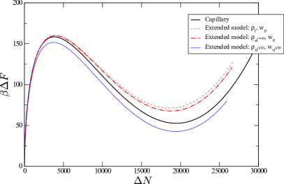
Figure 1: The free energy of cluster formation as a function of number of molecules inside the cluster at $S_{e}=1.125$ in a confined system of total volume, $V_{T}=4.5\times 10^{6}\sigma^{-3}$, using the modified capillary model with $\gamma$ being that calculated from infinite systems, and the extended model, with which we tested different combinations of the characteristic parameters $\rho_{0}$ and $w$. This graph shows the fact that the liquid phase is not stable so that nucleation will not proceed.

Figure 2: The Helmholtz free energy as a function of cluster size, $\Delta N$, at $S=1.175,\,1.5\$and $2.5$ for different cluster models. The left column are zooms of the figures on the right column about the critical size at each supersaturation. The right column shows the existence of a stable size behind which the energy of formation rockets. The total volume is again $V_{T}=4.5\times 10^{6}\sigma^{-3}$.

The work of cluster formation was evaluated by using equations (40) and (63) for the modified capillary and extended models respectively. Concerning the MCM, we fixed the surface tension to equal the CNT value calculated in the previous study for infinite systems,Lutsko and Durán-Olivencia (2013) i.e. $\gamma=\gamma_{\text{CNT}}$. However, the inner density $\rho_{0}$ was adjusted so as to minimize the free energy of the stable cluster, $\rho_{{st}^{(cap)}}$, unlike the classical capillary model where the inner density is set to be the that of the new phase, $\rho_{l}$. As for the extended model considering the PLP, we studied several possibilities to choose the characteristic parameters so that we can see more easily the effects of: the confinement, the interior density and the surface width. Thus, we tested three different combinations of the values $\rho_{0}$ and $w$:

1. Set the density $\rho_{0}=\rho_{l}$ and $w=w_{0}$ (from dCNT),

2. Set the density $\rho_{0}=\rho_{{st}^{(cap)}}$ and $w=w_{0}$,

3. Look for the pair $(\rho_{{st}^{(plp)}},w_{{st}^{(plp)}})$ to minimize the free energy (Eq. 63) of the stable cluster.

Figures 1 and 2 show the free energy landscapes at $S_{e}=1.125$ and $S_{e}=1.175,1.5,2.5$, respectively. The reason why the supersaturation values was divided into subsets is to highlight the fact that nucleation is inhibited in the first case while it still occurs in the other, as is obvious from these figures. On the one hand, in both cases we can observe the most important effect of considering confinement which is the emergence of a local (stable or metastable) minimum beyond the critical size as a result of finite mass. This is a new property which has no counterpart for an infinite system. Depending on the total amount of material, such a minimum will become metastable (Fig. 1) or stable (Fig. 2). On account of this fact a new effect arises, namely the control on the nucleation rate and the nucleation itself as a function of the total volume. Indeed, with the volume previously specified at $S_{e}=1.125$ no nucleation event will occur, given that the liquid (supposedly the new phase) is not stable any more. On the other hand, it is clear from those figures that the capillary model with a fixed $\gamma$ produces results close to those obtained with the extended models, at least up to $S_{e}=1.5$. In addition, we observe how the interface width plays a key role in the finite-width models lowering the energy of both the critical and the stable cluster, since $\rho_{st^{(cap)}}\simeq\rho_{st^{(plp)}}\simeq\rho_{l}$ (see Table 1). Indeed, what we found is that the width value which minimizes the stable-cluster energy is about twice the value $w_{0}$. There is also observed a great similarity of these results with respect to those for the infinite case, if we only pay attention on the left column of Fig. 2. Finally, in view of these results an interesting conclusion can be drawn in terms of experimental setups. The control on the total volume enables to modulate the stability of a given phase. This is an interesting result for crystallization experiments in small volumes (e.g. microfluidics), since it would imply that the effective solubility curve could be controlled at will.

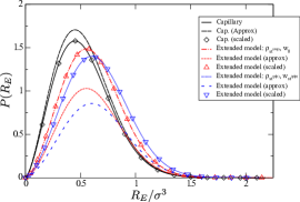
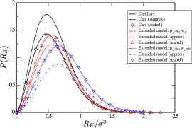
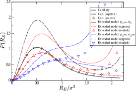
Figure 3: The stationary size distribution for the supersaturation values under which nucleation can proceed, $S_{e}=1.175$ (left panel), $S_{e}=1.5$ (center panel) and $S_{e}=2.5$ (right panel), with $V_{T}=4.5\times 10^{6}\sigma^{-3}$ and $R_{+}=1.5R_{*}$.

IV.2 The stationary distribution

A straightforward connection with experimental measurements can be made via the PDF which is essentially the quantity obtained by techniques like dynamic light scattering (DLS).Berne and Pecora (2000) Thus, the stationary PDF offers us another way to test the theories presented above. In addition, this quantity is required both in its exact (Eq. 23) and approximated (Eq. 35) form so as to determine the nucleation rate ans so we need to test its validity. In order to do that, we have to compute the PDF for the different models in terms of a common variable since $R$ does not mean the same thing in both of them, as we already pointed out. Thus, the calculations will be performed using the equimolar radius, $R_{E}$, which requires the transformation,

$$\overline{P}(R_{E})=P(R)\frac{dR}{dR_{E}},$$ (68)

with $R_{E}$ being equivalent to $R$ for the MCM or being given by equation (83) for the PLP.

The stationary size distributions are displayed in figure 3 showing good agreement with the results for the infinite case. The shape of the PDF is faithfully reproduced by the approximated equation (Eq. 24), at least for the lower effective supersaturations (left and center panels). However, the normalization is not equally well estimated, which is a result of the rapid change of the free energy with the cluster size for small clusters. Secondly, while for the MCM the approximation still remains being a good estimation for the highest density ($S_{e}=2.5$), a significant error arises for the extended models. The worse result lies on the extended model with a minimized stable cluster due to the fact that the system is in the pseudospinodal region,Xu et al. (2014) i.e. $\beta\Delta F_{*}\sim 1$, so that the assumption that small sizes govern the integral result is quite crude. Indeed, for these density values one would expect that cluster-cluster interactions play a key role thus violating the hypotheses assumed to make these calculations, as was noticed for infinite systems. Notwithstanding, we conclude that the capillary model exhibits a surprising ability to capture the main properties of nucleation even for finite systems.

IV.3 Nucleation rates

We end by comparing the nucleation (escape) rates in the different models previously introduced as shown in Table 1. It is apparent that for the lower densities the nucleation rates are much lower for the extended models with $w$ taken from dCNT calculations than for the capillary model, which is essentially due to the higher energy barrier associated with both of them. On the other hand, one observes the opposite situation when the extended model with a minimized stable cluster is considered, since the energy barrier is lower than that of the MCM (see Fig. 2). For the other cases the capillary approximation yields similar results to the extended models and to the CNT predictions. Next, we consider the variation of the nucleation rate as a function of volume. For the sake of simplicity, since a similar result in shape is obtained for each density we selected $S_{e}=1.5$. This calculation is shown in Fig. 4. A surprising effect is observed near the zero-rate zone, the nucleation rate exhibits a maximum for very small volumes and after that relaxes quickly to a steady value, which is nearly the one presented in Table 1. This is the result of a competition between two effects. On the one hand, the inner density of the cluster decreases with increasing total radius so that the bulk free energy increases. On the other hand, the free energy associated to the zone outside the cluster decreases when the total volume increases. It is therefore such a competition which causes a minimum in free-energy barrier and, hence, the maximum in nucleation rate. Before that maximum, the nucleation rate passes from being zero to non-zero in a very narrow region. From this result we can draw the conclusion that confined systems could be pretty well approximated by the infinite-system predictions, unless the volume under consideration is very close to the minimum volume for nucleation.

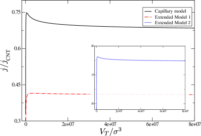
Figure 4: Nucleation rates as functions of the total volume at $S_{e}=1.5$. The extended models considered here are: 1) considering $\rho_{0}=\rho_{st^{(cap)}}$ and $w=w_{0}$, and 2) taking $\rho_{0}=\rho_{st^{(plp)}}$ and $w=w_{st^{(plp)}}$, i.e. those values which minimize the stable-cluster energy. It is observed how the confinement takes effect in a very narrow region, resulting in a maximum nucleation rate before inhibiting the process.

V Conclusions

In this work, a recent reformulation of classical nucleation theoryLutsko and Durán-Olivencia (2013) has been extended to consider finite systems. The motivation for making such an effort arises from the explosion of interest in nucleation process by using new techniques, such as microfluidics, where the hypotheses made by CNT are probably far from reality. Given that the dynamical reformulation of CNT was founded in a more fundamental framework, it was relatively easy to modify its derivation to take into account the mass-conservation law along with a finite volume and to go beyond the initial scope of CNT. With this goal attained, general expressions for both the stationary distribution function and the nucleation rate were obtained. Those were ultimately used with two different parametrized density profiles, a modified version of the capillary model to consider mass conservation and a piecewise-linear profile. Thus, the results obtained thereby allow to make a direct comparison to those performed for infinite systems.

The main conclusion we can draw from this study is that the nucleation rate can be somehow enhanced in a confined system. However, confinement affects in practice a very narrow range of volumes which is also why CNT produces good estimates. Surprisingly, the different profiles proposed here gave similar results where the main difference between them lies on the free energy barrier, as it also does for infinite systems. That said, it seems to us that the most natural way to further develop dCNT would be allowing the inner density to freely vary within the capillary model, which seems a good balance between being simple and accurate.

The nucleation rates were calculated in terms of the mean first-passage time,Hänggi et al. (1990); Wedekind et al. (2007); Lundrigan and Saika-Voivod (2009) which has been a widely used approach in this field. These calculations involved similar ingredients to those required to compute the stationary distribution function. The latter was evaluated numerically (Eq. 23) and by using its approximated version (Eq. 35). A good agreement between exact and approximated expressions were found for low and intermediate densities while for higher values the approximation became less accurate. Therefore, the same can be observed in the nucleation rates in Table 1. However, the fact that high densities yield worse approximations is not a key problem since certainly in such a regime the hypothesis of non-interacting clusters will be unlikely valid any more.

Finally, the volume of the system under study was varied in a wide range to study the effect on the nucleation rate. It was found that the finite volume effect is only noticeable for a narrow range of volumes and that it rapidly vanishes as the volume grows so that CNT and dCNT are accurate above this threshold.

Table 1: Properties of the capillary and extended cluster models as function of the effective supersaturation ratio, $S_{e}$ with $V_{T}=4.5\times 10^{6}\,\sigma^{-3}$. The absorbing wall was set to be $R_{+}=1.5\,R_{*}$.

		Modified Capillary Model
$S_{e}$	${j_{nc}}e^{-\Delta\beta F_{*}}$	$R_{*E}$	$\Delta N_{*}$	$\Delta\beta F_{*}$	$\frac{j}{{j_{nc}}}$	$\frac{j_{app}}{{j_{nc}}}$	$\rho_{0}$
1.175	0.695	7.94	1.22$\times 10^{3}$	80.8	0.198	0.191	0.66503
1.5	0.770	3.3	84.4	14.3	0.623	0.772	0.66438
2	1.532	2.15	21.9	6.06	0.548	0.834	0.66412
2.5	2.758	1.84	12.8	4.44	0.393	0.672	0.66401

		Extended model 0: $\rho_{0}=\rho_{l}$, $w=w_{0}$					Extended model 1: $\rho_{0}=\rho_{st^{(cap)}}$, $w=w_{0}$					Extended model 2: $\rho_{0}=\rho_{st^{(plp)}}$, $w=w_{st^{(plp)}}$
$S_{e}$	${j_{nc}}e^{-\Delta\beta F_{*}}$	$R_{*E}$	$\Delta N_{*}$	$\Delta\beta F_{*}$	$\frac{j}{{j_{nc}}}$	$\frac{j_{app}}{{j_{nc}}}$	$R_{*E}$	$\Delta N_{*}$	$\Delta\beta F_{*}$	$\frac{j}{{j_{nc}}}$	$\frac{j_{app}}{{j_{nc}}}$	$R_{*E}$	$\Delta N_{*}$	$\Delta\beta F_{*}$	$\frac{j}{{j_{nc}}}$	$\frac{j_{app}}{{j_{nc}}}$
1.175	0.695	8.03	933.25	81.9922	0.0041	0.0028	8.02	926.95	81.5787	0.0063	0.0043	7.83	787.32	75.2840	2.9234	1.7871
1.5	0.770	3.39	51.68	14.9410	0.0313	0.0272	3.39	51.37	14.7634	0.0380	0.0332	3.09	25.79	10.6570	1.6432	1.2196
2	1.532	2.16	10.57	5.8644	0.0903	0.1045	2.16	10.52	5.7515	0.1036	0.1205	1.82	2.97	2.8714	1.0116	1.0912
2.5	2.758	1.73	4.62	3.4804	0.1605	0.2349	1.73	4.60	3.3993	0.1799	0.2648	1.39	0.94	1.2245	1.0186	1.0338

			Extended model 0	Extended model 1		Extended model 2
$S_{e}$	$\rho_{l}$	${j_{nc}}/j_{\text{cnt}}$	$\frac{j}{j_{\text{cnt}}}$	$\rho_{0}$	$\frac{j}{j_{\text{cnt}}}$	$\rho_{0}$	$\frac{j}{j_{\text{cnt}}}$
1.175	0.665	0.47	0.0235	0.6650	0.0358	0.6636	16.73
1.5	0.665	1.15	0.3409	0.6644	0.4146	0.6635	17.91
2	0.665	1.63	1.0449	0.6641	1.1988	0.6634	11.71
2.5	0.665	2.57	2.3405	0.6640	2.6244	0.6634	14.86

Appendix A Calculations for the piecewise-linear profile

A.1 The cumulative mass and metric

Conforming to the postulated PLP, the cumulative mass can be computed for $0\leq R\leq w$,

$$m(r)= \Theta(R-r)\frac{\pi}{3w}(\rho_{0}-\rho_{ext}(R))r^{3}(4R-3r)$$

$$+\Theta(r-R)\frac{\pi}{3w}(\rho_{0}-\rho_{ext}(R))R^{4}$$

$$+V(r)\rho_{ext}(R)$$ (69)

while for $R>w$ it becomes,

$$m(r)= \Theta(R-w-r)V(r)(\rho_{0}-\rho_{ext}(R))$$

$$+\Theta(r-(R-w))\Theta(R-r)\times$$

$$\times\frac{\pi}{3w}(\rho_{0}-\rho_{ext}(R))\left(r^{3}(4R-3r)-(R-w)^{4}\right)$$

$$+\Theta(r-R)\frac{\pi}{3w}(\rho_{0}-\rho_{ext}(R))\left(R^{4}-(R-w)^{4}\right)$$

$$+V(r)\rho_{ext}(R)$$ (70)

with $V(r)=\frac{4\pi}{3}r^{3}$. According to these equations, the metric will present two contributions for those clusters with $0\leq R\leq w$ and three addends when $R>w$. In the first case,

$$g(R)=g_{i}(R)+g_{out}(R),\quad 0\leq R\leq w$$ (71)

with,

$$g_{i}(R)=\int_{0}^{R} \frac{1}{4\pi r^{2}\left(\rho_{0}-(\rho_{0}-\rho_{ext}(R))\frac{r-R+w}{w}\right)}\times$$

$$\times\left(\begin{array}[]{l}\frac{4\pi}{3w}r^{3}(\rho_{0}-\rho_{ext}(R))\\ \quad-\frac{\pi}{3w}(4R-3r)r^{3}\frac{\partial\rho_{ext}(R)}{\partial R}\\ \qquad+V(r)\frac{\partial\rho_{ext}(R)}{\partial R}\end{array}\right)^{2}dr,$$ (75)

$$g_{out}(R)=\int_{R}^{R_{T}} \frac{1}{4\pi r^{2}\rho_{ext}(R)}\times$$

$$\times\left(\begin{array}[]{l}\frac{4\pi}{3w}R^{3}(\rho_{0}-\rho_{ext}(R))\\ \quad-\frac{\pi}{3w}R^{4}\frac{\partial\rho_{ext}(R)}{\partial R}\\ \qquad+V(r)\frac{\partial\rho_{ext}(R)}{\partial R}\end{array}\right)^{2}\,dr.$$ (79)

The first term concerns the cluster surface and the second one affects to the outside mass. Although the exact solution exists and can be computed for these integrals, they are very crude. Fortunately, we are interested in obtaining an analytical approximation of the metric with the aim of calculating a first order approximation of $Y$ for small clusters. In this limit, it is a good estimation to consider $\rho_{ext}(R)\sim\rho_{av}$ and $\partial\rho_{ext}(R)/\partial R\sim 0$, giving rise to the expression already obtained for infinite systems,

$$g(R<w)\sim \frac{8\pi}{15}\left(\frac{\rho_{0}-\rho_{av}}{w}\right)^{2}\frac{R^{5}}{\rho_{av}}$$ (80)

The goodness of this approximation will be ultimately checked by comparison with the numerical results. For $R>w$ it also becomes an intractable equation whose solution is extremely crude. Thus, writing it down would be meaningless since our interest on the metric expression relies on finding an approximation of this quantity for small clusters.

Once again, a canonical variable can be defined and it can be expanded about small clusters,

$$Y(R)\sim \int_{0}^{R}\sqrt{g(R^{\prime}<w)}dR^{\prime}$$

$$\sim \frac{2}{7}\left(\frac{\rho_{0}-\rho_{av}}{w}\right)\sqrt{\frac{8\pi}{15\rho_{av}}}R^{7/2}$$ (81)

where the approximation (80) has been used. Given that quantity, now we can get the approximation for the excess number of molecules in the cluster, as we did previously. However, here $\Delta N$ has to be evaluated carefully as there is no a simple relation with $R$ as in the MCP, but with the equimolar radius $R_{E}$,

$$\Delta N= \int_{0}^{R_{T}}(\rho(\mathbf{r})-\rho_{ext}(R))d\mathbf{r}=\frac{4\pi}{3}R_{E}^{3}(\rho_{0}-\rho_{ext}(R)),$$ (82)

which in the case of the MCP is equivalent to $R$. After some manipulations one arrives at,

$$R_{E}^{3}={\left(\frac{1}{4w}\left(R^{4}-\left(\max(R-w,0)\right)^{4}\right)\right)}.$$ (83)

Therefore, the excess number of molecules will satisfy the following approximation for small clusters,

$$\Delta N\sim \frac{4\pi}{3}(\rho_{0}-\rho_{av})\frac{1}{4w}\left(\frac{7}{2}\left(\frac{w}{\rho_{0}-\rho_{av}}\right)\sqrt{\frac{15\rho_{av}}{8\pi}}\right)^{8/7}$$ (84)

A.2 Free energy

Now, as in the case of the metric, the work of cluster formation will have two different expressions depending on whether $R>w$ or $0\leq R\leq w$. Fortunately, an exact equation can be found in both cases, unlike for the metric. For $R>w$ equation (63) becomes,

$$\Delta\beta F(R;w)= \frac{4\pi}{3}(R-w)^{3}\beta\left(f(\rho_{0})-f(\rho_{av})\right)$$

$$+\left(1-\delta^{3}(R)\right)\,\beta\left(f(\rho_{ext}(R))-f(\rho_{av})\right)\,V_{T}$$

$$+4\pi\beta\left(\overline{\varphi}_{0}(R)w+K\frac{(\rho_{0}-\rho_{ext}(R))^{2}}{2w}\right)R^{2}$$

$$-4\pi\beta\left(2\overline{\varphi}_{1}(R)w+K\frac{(\rho_{0}-\rho_{ext}(R))^{2}}{2w}\right)Rw$$

$$+4\pi\beta\left(\overline{\varphi}_{2}(R)w+K\frac{(\rho_{0}-\rho_{ext}(R))^{2}}{6w}\right)w^{2},$$ (85)

with,

$$\overline{\varphi}_{k}(R;w)=\frac{\int_{\rho_{ext}(R)}^{\rho_{0}}\left(f(x)-f(\rho_{av})\right)\left(x-\rho_{ext}(R)\right)^{k}dx}{(\rho_{0}-\rho_{ext}(R))^{k+1}}.$$ (86)

It is easy to check that these expressions tend to their infinite-system counterparts when the corresponding limit is taken into account. Besides, the model reproduces the same similarity when the small cluster limit is imposed, i.e. for $R<w$,

$$\beta\Delta F(R;w) =\left(1-\delta^{3}(R)\right)\,\beta(f(\rho_{ext}(R))-f(\rho_{av}))\,V_{T}$$

$$+\int_{0}^{R}4\pi\,r^{2}\times$$

$$\times\beta\Delta f\left(\rho_{0}-(\rho_{0}-\rho_{ext}(R))\frac{r-R+w}{w}\right)dr$$

$$+\beta K\frac{2\pi}{3}R^{3}\left(\frac{\rho_{0}-\rho_{ext}(R)}{w}\right)^{2},$$ (87)

which can be eventually approximated by,

$$\beta\Delta F(R;w)\sim \beta K\frac{2\pi}{3}\left(\frac{\rho_{0}-\rho_{av}}{w}\right)^{2}R^{3}$$

$$\sim \frac{2\pi}{3}\beta K\left(\frac{\rho_{0}-\rho_{av}}{w}\right)^{2}$$

$$\times\left(\frac{7}{2}\left(\frac{w}{\rho_{0}-\rho_{av}}\right)\sqrt{\frac{15\rho_{av}}{8\pi}}\right)^{6/7}Y^{6/7},$$ (88)

equation which will be used to compute the nucleation rate subsequently, by using equation (34) with $\alpha=\frac{6}{7}$ and,

$$\widetilde{F}_{0}=\frac{2\pi}{3}\beta K\left(\frac{\rho_{0}-\rho_{av}}{w}\right)^{2}\left(\frac{7}{2}\left(\frac{w}{\rho_{0}-\rho_{av}}\right)\sqrt{\frac{15\rho_{av}}{8\pi}}\right)^{6/7}.$$ (89)