Quark matter subject to strong magnetic fields: phase diagram and applications

Abstract

In the present work we are interested in understanding various properties of quark matter subject to strong magnetic fields described by the Nambu–Jona-Lasinio model with Polyakov loop. We start by analysing the differences arising from two different vector interactions in the Lagrangian densities, at zero temperature, and apply the results to stellar matter. We then investigate the position of the critical end point for different chemical potential and density scenarios.

1 Introduction and Formalism

The study of the QCD phase diagram, when matter is subject to strong external magnetic fields has been a topic of intense investigation recently. The fact that magnetic fields can reach intensities of the order of $B\sim 10^{19}$ G or higher in heavy-ion collisions [1] and up to $10^{18}$ G in the center of magnetars [2] made theoretical physicists consider matter subject to magnetic field both at high temperatures and low densities and low temperatures and high densities.

In this work we study the above mentioned situations within the framework of the Nambu–Jona-Lasinio model with Polyakov Loop (PNJL) and different versions of the Nambu–Jona-Lasinio (NJL) model [3] for two commonly used parameter sets, known as HK [4] and RKH [5].

We describe quark matter subject to strong magnetic fields within the SU(3) PNJL model with vector interaction and the Lagrangian density reads:

$${\cal L} = {\bar{\psi}}_{f}\left[i\gamma_{\mu}D^{\mu}-{\hat{m}}_{f}\right]\psi_{f}~{}+~{}{\cal L}_{sym}~{}+~{}{\cal L}_{det}$$ (1)

$$+ {\cal L}_{vec}+{\mathcal{U}}\left(\Phi,\bar{\Phi};T\right)-\frac{1}{4}F_{\mu\nu}F^{\mu\nu},$$

with

$${\cal L}_{sym} = G\sum_{a=0}^{8}\left[({\bar{\psi}}_{f}\lambda_{a}\psi_{f})^{2}+({\bar{\psi}}_{f}i\gamma_{5}\lambda_{a}\psi_{f})^{2}\right],$$

$${\cal L}_{det} = -K\left\{{\rm det}_{f}\left[{\bar{\psi}}_{f}(1+\gamma_{5})\psi_{f}\right]+{\rm det}_{f}\left[{\bar{\psi}}_{f}(1-\gamma_{5})\psi_{f}\right]\right\},$$

where $\psi_{f}=(u,d,s)^{T}$ represents a quark field with three flavors, ${\hat{m}}_{c}={\rm diag}_{f}(m_{u},m_{d},m_{s})$ is the corresponding (current) mass matrix, $\lambda_{0}=\sqrt{2/3}I$ where $I$ is the unit matrix in the three flavor space, and $0<\lambda_{a}\leq 8$ denote the Gell-Mann matrices. The coupling between the magnetic field $B$ and quarks, and between the effective gluon field and quarks is implemented via the covariant derivative $D^{\mu}=\partial^{\mu}-iq_{f}A_{EM}^{\mu}-iA^{\mu}$ where $q_{f}$ represents the quark electric charge, $A^{EM}_{\mu}=\delta_{\mu 2}x_{1}B$ is a static and constant magnetic field in the $z$ direction and $F_{\mu\nu}=\partial_{\mu}A^{EM}_{\nu}-\partial_{\nu}A^{EM}_{\mu}$. To describe the pure gauge sector an effective potential ${\mathcal{U}}\left(\Phi,\bar{\Phi};T\right)$ is chosen:

$$\frac{{\mathcal{U}}\left(\Phi,\bar{\Phi};T\right)}{T^{4}}=-\frac{a\left(T\right)}{2}\bar{\Phi}\Phi\\ +\,b(T)\mbox{ln}\left[1-6\bar{\Phi}\Phi+4(\bar{\Phi}^{3}+\Phi^{3})-3(\bar{\Phi}\Phi)^{2}\right],$$

where $a\left(T\right)=a_{0}+a_{1}\left(\frac{T_{0}}{T}\right)+a_{2}\left(\frac{T_{0}}{T}\right)^{2}$, $b(T)=b_{3}\left(\frac{T_{0}}{T}\right)^{3}$. The standard choice of the parameters for the effective potential $\mathcal{U}$ is $a_{0}=3.51$, $a_{1}=-2.47$, $a_{2}=15.2$, and $b_{3}=-1.75$.

As for the vector interaction, the Lagrangian density that denotes the $U(3)_{V}\otimes U(3)_{A}$ invariant interaction is

$${\cal L}_{vec}=-G_{V}\sum_{a=0}^{8}\left[({\bar{\psi}}\gamma^{\mu}\lambda_{a}\psi)^{2}+({\bar{\psi}}\gamma^{\mu}\gamma_{5}\lambda_{a}\psi)^{2}\right],$$ (2)

and a reduced Lagrangian density can be written as

$${\cal L}_{vec}=-G_{V}({\bar{\psi}}\gamma^{\mu}\psi)^{2}.$$ (3)

At zero temperature the PNJL model reduces to the normal NJL model.

In the SU(3) models, the above Lagrangian densities for the vector sector are not identical in a mean field approach and we discuss both cases next. We refer to the Lagrangian density given in Eq. (2) as model 1 (P1) and to the Lagrangian density given in Eq. (3) as model 2 (P2).

For our calculations, we need to evaluate the thermodynamical potential for the three flavor quark sector, $\Omega=-P={\cal E}-T{\cal S}-\sum_{f}{\mu_{f}}\rho_{f}$ where $P$ represents the pressure, ${\cal E}$ the energy density, $T$ the temperature, ${\cal S}$ the entropy density, and ${\mu_{f}}$ the chemical potential of quark with flavor $f$. To determine the EOS for the SU(3) NJL at finite density and in the presence of a magnetic field in a mean field approximation we need to know the scalar condensates, $\phi_{f}$, the quark number densities, $\rho_{f}$, as well as the pressure kinetic contribution from the gas of quasi-particles, $\theta_{f}$. In the presence of a magnetic field all these quantities have been evaluated with great detail in [6, 7].

2 $T=0$ - quark and stellar matter

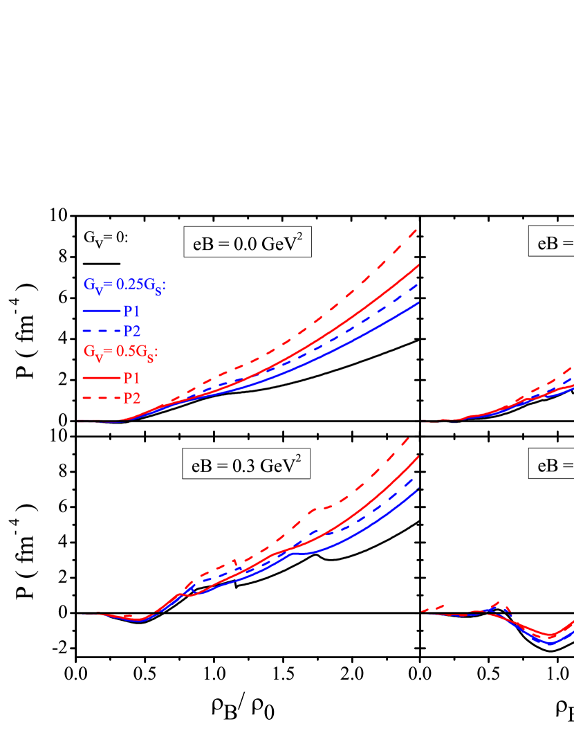
Figure 1: Pressure versus baryonic density for equal chemical potentials and models P1 and P2 for different values of $G_{V}/G_{S}$, and several intensities of the magnetic field. Figure taken from [10].

We next restrict ourselves to the NJL model with vector interaction, disregarding the Polyakov loop, which has shown to be important at finite temperature only. The effect of the vector interaction on three flavor magnetized matter is studied for cold matter within the two different models mentioned above, a flavor dependent (P1) [8] and a flavor independent one (P2) [9].

If model P1 is considered, the pressure reads:

$$P=\theta_{u}+\theta_{d}+\theta_{s}-2G_{S}(\phi_{u}^{2}+\phi_{d}^{2}+\phi_{s}^{2})+2G_{V}(\rho_{u}^{2}+\rho_{d}^{2}+\rho_{s}^{2})+4K\phi_{u}\phi_{d}\phi_{s}\,\,,$$ (4)

and the effective chemical potential, for each flavor, is given by

$${\tilde{\mu}}_{i}=\mu_{i}-4G_{V}\rho_{i}.\quad i=u,d,s$$ (5)

We also refer to P1 as the flavor dependent model, for the reasons that will become obvious from the analysis of our results.

If, on the other hand, model P2 is considered, the pressure becomes:

$$P=\theta_{u}+\theta_{d}+\theta_{s}-2G_{S}(\phi_{u}^{2}+\phi_{d}^{2}+\phi_{s}^{2})+G_{V}\rho^{2}+4K\phi_{u}\phi_{d}\phi_{s}\,\,,$$ (6)

where

$$\rho=\rho_{u}+\rho_{d}+\rho_{s},\quad\rho_{B}=\rho/3,$$ (7)

and in this case the effective chemical potential, for each flavor, is given by

$${\tilde{\mu}}_{i}=\mu_{i}-2G_{V}\rho.$$ (8)

We next refer to P2 as the flavor independent (or flavor blind) model.

The effect of the magnetic field on the EOS can be seen in Figure 1 for the case when $\mu_{u}=\mu_{d}=\mu_{s}$. The van-Alphen oscillations due to the filling of the Landau levels are already seen for $eB=0.1$ GeV². The softening occurring when a new Landau level starts being occupied has a strong effect at the smaller densities giving rise to a pressure that is negative within a larger range of densities.

As can be seen in Figure 2, the flavor independent vector interaction predicts a smaller strangeness content and, therefore, harder equations of state. Moreover, the strangeness content does not depend on the strength of the vector interaction. On the other hand, the flavor dependent vector interaction favors larger strangeness content the larger the vector coupling,

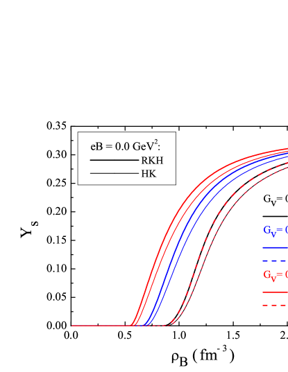
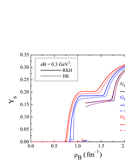
Figure 2: The strangeness fraction as a function of the baryonic density for models P1 and P2 and different values of $G_{V}$, and $B=0$ (left panel); $eB=0.3$ GeV² (right panel). Figure taken from [10].

We now move to the study of quark and hybrid stars subject to an external magnetic field. In these cases, $\beta$-equilibrium conditions and charge neutrality are enforced. Mass-radius curves are shown in Figure 3 for both star types with the RKH parameter set. The hadronic phase in hybrid stars was obtained with the GM1 parametrization of the non-linear Walecka model [11]. A Maxwell construction was then used.

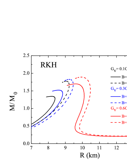
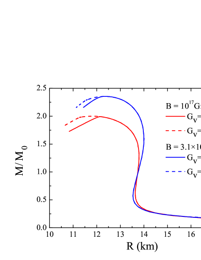
Figure 3: Mass radius curves obtained with P2 for different values of $G_{V}$, two intensities of the magnetic field, parametrization RKH for quark (left panel) and hybrid stars (right panel). Figure taken from [10].

			HK			RKH
			$x=0.1$	$x=0.3$	$x=0.6$	$x=0.1$	$x=0.3$	$x=0.6$
$B=0$ G	P1	$M_{max}$ ($M_{0}$)	1.49	1.58	1.69	1.27	1.35	1.46
		R (km)	9.13	10.89	11.98	8.01	8.17	9.41
		$\varepsilon_{c}$ ($\mathrm{fm}^{-4}$)	7.23	6.96	6.52	9.42	9.61	9.84
	P2	$M_{max}$ ($M_{0}$)	1.56	1.72	1.91	1.35	1.54	1.74
		R (km)	9.15	10.61	11.47	8.22	8.60	9.91
		$\varepsilon_{c}$ ($\mathrm{fm}^{-4}$)	7.35	7.37	6.92	8.71	8.58	8.09
$B=10^{17}$ G		$M_{max}$ ($M_{0}$)	1.56	1.72	1.91	1.35	1.54	1.74
P2		R (km)	9.16	10.16	10.95	8.21	8.58	9.60
		$\varepsilon_{c}$ ($\mathrm{fm}^{-4}$)	7.41	7.36	6.98	8.80	8.94	8.11
$B=3.1\times 10^{18}$ G		$M_{max}$ ($M_{0}$)	1.96	2.03	2.12	1.81	1.88	1.98
P2		R (km)	9.98	10.43	11.05	9.03	9.21	9.90
		$\varepsilon_{c}$ ($\mathrm{fm}^{-4}$)	7.41	7.22	6.78	8.74	8.21	7.80

Table 1: Stellar macroscopic properties obtained from EOS of non-magnetized matter for models P1 and P2 and for magnetized matter with model P2. $M_{max}$ is the maximum mass, R is the star radius, $\varepsilon$ the star central energy density and $x=G_{V}/G_{S}$. Table taken from [10].

From Table 1 we can see that larger star masses are obtained for the flavor independent vector interaction and maximum masses of the order of 2 $M_{\odot}$ can be achieved depending on the value of the vector interaction and on the intensity of the magnetic field.

HK		$M_{max}$	$M_{b}$	R	$\varepsilon_{c}$	$\varepsilon$ (onset)	$\mu_{B}(\varepsilon_{c})$	$\mu_{B}$ (onset)
		($M_{0}$)	($M_{0}$)	(km)	($\mathrm{fm}^{-4}$)	($\mathrm{fm}^{-4}$)	(MeV)	(MeV)
$B=10^{17}$ G	$x=0$	1.91	2.18	12.78	4.57	3.47	1360	1330
P2	$x=0.10$	1.99	2.30	12.14	6.27	5.05	-	1503
	$x=0.22$	2.00	2.31	11.82	5.93	7.79	1580	1726
$B=3.1\times 10^{18}$ G	$x=0$	2.27	2.60	12.82	4.69	3.30	1324	1261
P2	$x=0.10$	2.35	2.70	12.34	5.29	5.59	1427	1453
	$x=0.22$	2.35	2.70	12.35	5.27	9.03	1426	1730
RKH		$M_{max}$	$M_{b}$	R	$\varepsilon_{c}$	$\varepsilon$ (onset)	$\mu_{B}(\varepsilon_{c})$	$\mu_{B}$ (onset)
		($M_{0}$)	($M_{0}$)	(km)	($\mathrm{fm}^{-4}$)	($\mathrm{fm}^{-4}$)	(MeV)	(MeV)
$B=10^{17}$ G	$x=0$	1.97	2.26	12.48	4.29	4.28	-	1422
P2	$x=0.10$	2.00	2.31	11.91	7.51	5.67	-	1557
	$x=0.19$	2.00	2.31	11.83	5.91	7.83	1579	1728
$B=3.1\times 10^{18}$ G	$x=0$	2.33	2.69	12.79	4.69	4.19	-	1335
P2	$x=0.10$	2.35	2.70	12.34	5.30	6.52	1428	1531
	$x=0.19$	2.35	2.70	12.34	5.30	9.05	1428	1731

Table 2: Stellar macroscopic properties obtained from EOS of magnetized hybrid stars built with GM1 and SU(3) NJL with HK and RKH parametrizations. $M_{max}$ is the maximum gravitational mass, $M_{b}$ is the maximum baryonic mass, $R$ is the star radius, $\varepsilon_{c}$ is the star central energy density, $\mu_{B}(\varepsilon_{c})$ is the chemical potential for neutron at $\varepsilon_{c}$ and $\mu_{B}$(onset) is the baryonic chemical potential at the onset of the quark phase. Results taken from [10].

From the results displayed in Table 2, we observe that hybrid stars may bare a core containing deconfined quarks if neither the vector interaction nor the magnetic field are too strong. The onset of the quark phase as compared with the central values for the energy density and related chemical potential show that quarks would appear only at densities/chemical potentials larger than the existing ones in the stellar core. The presence of strong magnetic fields also disfavor the existence of a quark core in hybrid stars.

3 Critical end point within the PNJL model

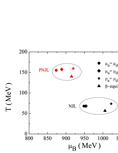
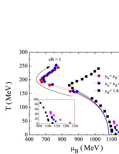
Figure 4: Left panel - Location of the CEP on a diagram $T$ vs the baryonic chemical potential under different scenarios and models (NJL, PNJL). No external magnetic field is considered. Right panel - Effect of an external magnetic field on the CEP location within PNJL model for three different scenarios. Figure taken from [13].

We move next to finite temperature and study the location of the critical end point (CEP) on the QCD phase diagram within the framework of the PNJL model and without the introduction of the vector interaction. We investigate different scenarios with respect to the isospin and strangeness content of matter, as shown in Figure 4 left for non-magnetized matter. For matter in $\beta$-equilibrium, the CEP occurs at smaller temperatures and densities. This scenario is of interest for neutron stars and confirms previous calculations that indicate that a deconfinement phase transition in the laboratory will be more easily attained with asymmetric nuclear matter [12].

As a matter of fact, by taking $\mu_{s}=0$ and increasing systematically $\mu_{d}$ with respect to $\mu_{u}$ the CEP moves to smaller temperatures and larger baryonic chemical potentials [13]: less symmetric matter is less bound and, therefore, the transition to a chirally symmetric phase occurs at a smaller temperature and density than in the symmetric case ($\mu_{u}=\mu_{d}=\mu_{s}$). When the asymmetry is large enough, $\mu_{d}=1.45~{}\mu_{u}$, the CEP disappears.

Another interesting situation is observed when analyzing very isospin asymmetric matter subject to different intensities of the magnetic field, as seen in Figure 4 right. Starting from a scenario having an isospin asymmetry above which the CEP does not exist for a zero external magnetic field ($\mu_{d}=1.45~{}\mu_{u}$) it was shown the introduction of an external magnetic field could drive the system to a first order phase transition. The CEP occurs at very small temperatures if $eB<0.1$ GeV² and, in this case, a complicated structure with several CEP at different values of ($T,\mu_{B})$ are possible for the same magnetic field, because the temperature is not high enough to wash out the Landau level effects. Indeed, the magnetic field affects in a different way $u$ and $d$ quarks due to their different electric charge. A consequence is the possible appearance of two or more CEPs for a given magnetic field intensity. For $eB>0.1$ GeV² only one CEP exists. This is an important result because it shows that an external magnetic field is able to drive a system with no CEP into a first order phase transition [13].

In the right panel of Figure 4 we present the results for two other scenarios where a first order phase transition already occurs at zero magnetic field: $\mu_{u}=\mu_{d}=\mu_{s}$ and $\mu_{u}=\mu_{d}\,\&\,\mu_{s}=0$. For moderate magnetic fields the trend is very similar for all scenarios: as the intensity of the magnetic field increases, the transition temperature increases and the baryonic chemical potential decreases until the critical value $eB\sim 0.4$ GeV². For stronger magnetic fields both $T$ and $\mu_{B}$ increase.

It is also important to point out that all three scenarios presented in the right panel of Figure 4 show an inverse magnetic catalysis at finite chemical potential and zero temperature, i.e., the critical temperature decreases with increasing $eB$. For large values of $eB$ this inverse magnetic catalysis tendency disappears and a magnetic catalysis takes place.

Acknowledgements: This work was partially supported by CNPq (Brazil), CAPES (Brazil) and FAPESC (Brazil) under Project 2716/2012,TR 2012000344, by Project No. PTDC/FIS/113292/2009 developed under the initiative QREN financed by the UE/FEDER through the program COMPETE —”Programa Operacional Factores de Competitividade,” by Grant No. SFRH/BD/51717/2011 (F.C.T.) and by NEW COMPSTAR, a COST initiative.

References

- [1] V. Skokov, A. Y. Illarionov and V. Toneev, Int. J. Mod. Phys. A 24, 5925 (2009).
- [2] R. Duncan and C. Thompson, Astrophys. J. 392 L9 (1992); C. Kouveliotou et al., Nature (London) 393 235 (1998).
- [3] Y. Nambu and G. Jona-Lasinio, Phys. Rev. 122, 345 (1961); 124, 246 (1961).
- [4] T. Hatsuda and T. Kunihiro, Phys. Rep. 247, 221 (1994).
- [5] P. Rehberg, S. P. Klevansky and J. Hüfner, Phys. Rev. C 53, 410 (1996).
- [6] D.P. Menezes, M. Benghi Pinto, S.S. Avancini, A. Pérez Martinez and C. Providência, Phys. Rev. C 79, 035807 (2009).
- [7] S.S. Avancini, D.P. Menezes, M.B. Pinto and C. Providência, Phys. Rev. C 80, 065805 (2009).
- [8] S. Klimt, M. Lutz, and W. Weise, Phys. Lett. B249, 386 (1990); M. Hanauske, L. M. Satarov, I. N. Mishustin, H. Stöcker and W. Greiner, Phys. Rev. D 64, 043005 (2001).
- [9] K. Fukushima, Phys. Rev. D 78, 114019 (2008).
- [10] Debora P. Menezes, Marcus B. Pinto, Luis R. B de Castro, Constança Providencia and Pedro Costa, Phys. Rev. C 89, 055207 (2014).
- [11] N. K. Glendenning, Compact Stars, Springer, New York (2000).
- [12] R. Cavagnoli, C. Providência and D. P. Menezes, Phys. Rev. C 83, 045201 (2011).
- [13] Pedro Costa, Márcio Ferreira, Hubert Hansen, Débora P. Menezes, Constança Providência, Phys. Rev. D 89, 056013 (2014).