Possibilities for reduction of transverse projected emittances
by partial removal of transverse to longitudinal beam correlations

Abstract

We show that if in the particle beam there are linear correlations between energy of particles and their transverse positions and momenta (linear beam dispersions), then the transverse projected emittances always can be reduced by letting the beam to pass through magnetostatic system with specially chosen nonzero lattice dispersions. The maximum possible reduction of the transverse projected emittances occurs when all beam dispersions are zeroed, and the values of the lattice dispersions required for that are completely defined by the values of the beam dispersions and the beam rms energy spread and are independent from any other second-order central beam moments. Besides that, we prove that, alternatively, one can also use the lattice dispersions to remove linear correlations between longitudinal positions of particles and their transverse coordinates (linear beam tilts), but in this situation solution for the lattice dispersions is nonunique and the reduction of the transverse projected emittances is not guaranteed.

I Introduction

Careful control of the beam quality is essential for linear accelerators designed to deliver very high brightness electron beams for short wavelength free electron lasers (FELs). There are many beam properties which have to be observed and manipulated such as suppression of microbunching instability, creation of needed peak current, preservation of slice and projected emittances, etc.

In this paper we are interested in some aspects of the control of transverse projected emittances. Among the sources of the growth of transverse projected emittances are the incoherent and coherent synchrotron radiation (CSR) withing magnetic bunch compressors as well as the other wake fields along the accelerator. A number of approaches which could help to reduce emittance growth due to CSR wake during bunch compression were developed during last decades including different optics tricks, preparation of the initial beam current profile at the bunch compressor entrance and etc. (see, for example,  LouMos ; DohL ; SdiM ; JHL ; MQE and references therein).

Still, because the suggested schemes provide reduction but not complete cancellation of the emittance growth, the beam considered downstream of the compression system (or at the linac exit) could have nonzero transverse to longitudinal coupling terms in the beam matrix and therefore projected emittances could be further reduced if these correlations will be removed.

In general, in order to make complete transverse to longitudinal decoupling, it is necessary to have the possibility to act on particles depending on their longitudinal position within the bunch (for example, one may involve transverse deflecting cavities for this purpose), which means that the system designed for the complete decoupling could be too complicated and somewhat difficult to operate in comparison with the benefit coming from the achievable reduction of the transverse projected emittances.

In this paper we consider a more simple and more practical question: what one can do having at hand a magnetostatic correction system? Because the transfer matrix of a magnetostatic system could couple transverse and longitudinal particle coordinates only when the dispersions of the underlying magnetic structure are nonzero, the reduction of transverse projected emittances (if any possible) will always be accompanied by the creation of a potential source of beam transverse jitter due to the beam energy jitter, and one has to look for an appropriate balance of both.

We show, in the framework of linear particle dynamics and with the self field effects neglected, that if in the beam matrix there are nonzero correlation terms between energy of particles and their transverse positions and momenta (beam dispersions), then the transverse projected emittances can be reduced by letting the beam pass through magnetostatic system (correction system) with specially chosen nonzero lattice dispersions. The maximum possible reduction of the transverse projected emittances occurs when all beam dispersions are zeroed, and the values of the lattice dispersions required for that are completely determined by the values of the beam dispersions and the beam rms energy spread and are independent from any other second-order central beam moments. Besides that, we prove that, alternatively, one can also use the lattice dispersions to remove linear correlations between longitudinal positions of particles and their transverse coordinates (beam tilts), but in this situation solution for the lattice dispersions is nonunique and the reduction of the transverse projected emittances is not guaranteed.

Note that this paper is an extended version of the unpublished note My00 , which was written during discussion of the influence of different dispersive effects on the performance of the FLASH facility Flash01 ; Flash02 , and recently, when we get acquainted with the paper PSI , our interest to this problem was renewed. Both papers, My00 and PSI , employ unclosed lattice dispersions as a tuning knob for the control of the transverse projected emittances, but have somewhat different points of view on the practical realization of this idea and therefore the direct comparison of their results and recommendations is not very straightforward. As far as we are mostly discussing possibilities for correction which can be made downstream of the emittance growth and coupling source either by means of a dedicated correction system or even simply by special (dispersive) beam steering, the paper PSI suggests to create dispersion nonclosure already in the bunch compressor, where the CSR effect is strongest and can not be neglected.

II Variables and notations

We consider the linear beam dynamics in an electromagnetic system which conserves the reference beam energy and take the path length along the reference orbit $\tau$ to be the independent variable. We use a complete set of symplectic variables

$$\mbox{\boldmath$z$}=(x,p_{x},y,p_{y},\sigma,\varepsilon)^{\top}$$ (1)

as particle coordinates MaisRipken ; My01 . Here $x,\,y$ measure the transverse (horizontal and vertical) displacements from the ideal orbit and $p_{x},\,p_{y}$ are the corresponding canonical monenta scaled with the constant kinetic momentum of the reference particle $p_{0}$. The variables $\sigma$ and $\varepsilon$ which describe the longitudinal dynamics are

$$\sigma=c\,\beta_{0}\,(t_{0}-t),\quad\varepsilon=({\cal{E}}-{\cal{E}}_{0})\,/\,(\beta_{0}^{2}\,{\cal{E}}_{0}),$$ (2)

where ${\cal{E}}_{0},\,\beta_{0}$ and $t_{0}=t_{0}(\tau)$ are the energy of the reference particle, its velocity in terms of the speed of light $c$ and its arrival time at a certain position $\tau$, respectively.

Let $M$ be an $m\times m$ square matrix. Then $\left|M\right|$ denote the determinant of $M$. Let $\omega$ be a nonempty subset of $\{1,2,\ldots,m\}$ with its elements listed in increasing order. Then $M\{\omega\}$ denote the principal submatrix of $M$ whose entries are in the intersection of those rows and columns of $M$ specified by $\omega$. If $M$ is a symmetric matrix, we denote by $\Psi_{M}$ the associated with this matrix quadratic form in $m$-variables $u_{1},\ldots,u_{m}$

$$\Psi_{M}(u_{1},\ldots,u_{m})=(u_{1},\ldots,u_{m})\cdot M\cdot(u_{1},\ldots,u_{m})^{\top}.$$ (3)

Besides that, we denote by $I_{m}$ the $m\times m$ identity matrix and by

$$J_{2m}\;=\;\mbox{diag}\Bigg{(}\underbrace{\left(\begin{array}[]{rr}0&1\\ -1&0\end{array}\right),\ldots,\left(\begin{array}[]{rr}0&1\\ -1&0\end{array}\right)}_{m}\Bigg{)}$$ (8)

the $2m\times 2m$ symplectic unit matrix.

As usual, we describe the properties of a collection of points (a particle beam) in the three degrees of freedom (3D) phase space by a $6\times 6$ symmetric matrix (beam matrix) of the second-order central beam moments

$$\Sigma=\left\langle\left(\mbox{\boldmath$z$}-\langle\mbox{\boldmath$z$}\rangle\right)\left(\mbox{\boldmath$z$}-\langle\mbox{\boldmath$z$}\rangle\right)^{\top}\right\rangle,$$ (9)

where the brackets $\langle\,\cdot\,\rangle$ denote an average over a distribution of the particles in the beam.

Let $R$ be the nondegenerated $6\times 6$ matrix which propagates particle coordinates from the state $\tau=s_{1}$ to the state $\tau=s_{2}$, i.e let

$$\mbox{\boldmath$z$}(s_{2})\,=\,R\,\mbox{\boldmath$z$}(s_{1}).$$ (10)

Then from (9) and (10) it follows that the matrix $\Sigma$ evolves between these two states according to the congruence

$$\Sigma(s_{2})\,=\,R\,\Sigma(s_{1})\,R^{\top}.$$ (11)

In the following we assume that the beam transport matrix $R$ is symplectic, which is equivalent to say that it satisfies the relation

$$R^{\top}J_{6}\,R\,=\,J_{6}.$$ (12)

By definition, the beam matrix $\Sigma$ is symmetric positive semidefinite and we restrict our considerations to the situation when this matrix is nondegenerated and therefore positive definite. For simplification of notations we also assume that the beam is proper centered and therefore has vanishing first-order moments $\big{<}\mbox{\boldmath$z$}\big{>}=0$. With this assumption the beam matrix takes on the form

$$\Sigma=\left(\begin{array}[]{cccccc}\langle x^{2}\rangle&\langle xp_{x}\rangle&\langle xy\rangle&\langle xp_{y}\rangle&\langle x\sigma\rangle&\langle x\varepsilon\rangle\\ \langle xp_{x}\rangle&\langle p_{x}^{2}\rangle&\langle yp_{x}\rangle&\langle p_{x}p_{y}\rangle&\langle p_{x}\sigma\rangle&\langle p_{x}\varepsilon\rangle\\ \langle xy\rangle&\langle yp_{x}\rangle&\langle y^{2}\rangle&\langle yp_{y}\rangle&\langle y\sigma\rangle&\langle y\varepsilon\rangle\\ \langle xp_{y}\rangle&\langle p_{x}p_{y}\rangle&\langle yp_{y}\rangle&\langle p_{y}^{2}\rangle&\langle p_{y}\sigma\rangle&\langle p_{y}\varepsilon\rangle\\ \langle x\sigma\rangle&\langle p_{x}\sigma\rangle&\langle y\sigma\rangle&\langle p_{y}\sigma\rangle&\langle\sigma^{2}\rangle&\langle\sigma\varepsilon\rangle\\ \langle x\varepsilon\rangle&\langle p_{x}\varepsilon\rangle&\langle y\varepsilon\rangle&\langle p_{y}\varepsilon\rangle&\langle\sigma\varepsilon\rangle&\langle\varepsilon^{2}\rangle\end{array}\right)$$ (19)

where the elements

$$\langle x\varepsilon\rangle,\quad\langle p_{x}\varepsilon\rangle,\quad\langle y\varepsilon\rangle,\quad\langle p_{y}\varepsilon\rangle$$ (20)

and the elements

$$\langle x\sigma\rangle,\quad\langle p_{x}\sigma\rangle,\quad\langle y\sigma\rangle,\quad\langle p_{y}\sigma\rangle$$ (21)

we call beam dispersions and beam tilts, respectively.

The matrix $\Sigma$ has twenty-one different entries which can be varied independently within the positive definiteness conditions. Of course, not all of them (or their combinations) are equally interesting for any particular accelerator physics application. In this paper we concentrate on the study of the evolution of 1D horizontal, vertical and longitudinal projected emittances

$$\varepsilon_{x}=\left|\Sigma\left\{1,2\right\}\right|^{1/2},$$ (22)

$$\varepsilon_{y}=\left|\Sigma\left\{3,4\right\}\right|^{1/2},$$ (23)

$$\varepsilon_{\sigma}=\left|\Sigma\left\{5,6\right\}\right|^{1/2},$$ (24)

and 2D transverse projected emittance

$$\varepsilon_{t}=\left|\Sigma\left\{1,2,3,4\right\}\right|^{1/2}$$ (25)

under the transformation rule (11) with the additional assumption that the matrix $R$ is the transport matrix of a magnetostatic system. Besides that, we also pay attention to the changes in the beam energy chirp $\langle\sigma\varepsilon\rangle$ (linear energy slope along the bunch length) and in the rms bunch length squared $\langle\sigma^{2}\rangle$.

Note that due to Hadamar’s determinantal inequality

$$\varepsilon_{t}\,\leq\,\varepsilon_{x}\,\varepsilon_{y},$$ (26)

and the equality in (26) holds if and only if the transverse degrees of freedom in the beam matrix are decoupled from each other HornJohnson , i.e. if and only if

$$\langle xy\rangle=\langle xp_{y}\rangle=\langle yp_{x}\rangle=\langle p_{x}p_{y}\rangle=0.$$ (27)

III Transport of beam matrix through magnetostatic system

III.1 Matrix of a magnetostatic system

The most general form of the transport matrix of a magnetostatic system is

$$R=\left(\begin{array}[]{cccccc}r_{11}&r_{12}&r_{13}&r_{14}&0&r_{16}\\ r_{21}&r_{22}&r_{23}&r_{24}&0&r_{26}\\ r_{31}&r_{32}&r_{33}&r_{34}&0&r_{36}\\ r_{41}&r_{42}&r_{43}&r_{44}&0&r_{46}\\ r_{51}&r_{52}&r_{53}&r_{54}&1&r_{56}\\ 0&0&0&0&0&1\end{array}\right),$$ (34)

where the elements

$$r_{16},\;r_{26},\;r_{36},\;r_{46},\;r_{51},\;r_{52},\;r_{53},\;r_{54},\;r_{56}$$ (35)

are (transverse and longitudinal) lattice dispersions.

The special form (34) of the matrix $R$ allows to rewrite the symplecticity condition (12) in the form of a system of two equations

$$\left(R\{1,2,3,4\}\right)^{\top}J_{4}\,\left(R\{1,2,3,4\}\right)\,=\,J_{4}$$ (36)

and

$$\left(\begin{array}[]{c}r_{16}\\ r_{26}\\ r_{36}\\ r_{46}\end{array}\right)\,=\,\left(R\{1,2,3,4\}\right)J_{4}\left(\begin{array}[]{c}r_{51}\\ r_{52}\\ r_{53}\\ r_{54}\end{array}\right),$$ (45)

and using condition (45) one can show that every matrix $R$ of the form (34) can be represented as a product

$$R\,=\,R_{1}\,R_{2},$$ (46)

where

$$R_{1}=\left(\begin{array}[]{cccccc}r_{11}&r_{12}&r_{13}&r_{14}&0&0\\ r_{21}&r_{22}&r_{23}&r_{24}&0&0\\ r_{31}&r_{32}&r_{33}&r_{34}&0&0\\ r_{41}&r_{42}&r_{43}&r_{44}&0&0\\ 0&0&0&0&1&0\\ 0&0&0&0&0&1\end{array}\right)$$ (53)

is the dispersion-free part of the matrix $R$ and

$$R_{2}=\left(\begin{array}[]{cccccc}1&0&0&0&0&\;\;\,r_{52}\\ 0&1&0&0&0&-r_{51}\\ 0&0&1&0&0&\;\;\,r_{54}\\ 0&0&0&1&0&-r_{53}\\ r_{51}&r_{52}&r_{53}&r_{54}&1&\;\;\,r_{56}\\ 0&0&0&0&0&\;\;\,1\end{array}\right)$$ (60)

is its dispersive part.

Substituting the decomposition (46) into the beam matrix propagation equation (11) one obtains

$$\Sigma(s_{2})\,=\,R_{1}\,\left(R_{2}\,\Sigma(s_{1})\,R_{2}^{\top}\right)R_{1}^{\top}.$$ (61)

This formula is a two step transformation. At first the incoming beam matrix $\Sigma(s_{1})$ is transported using the matrix $R_{2}$ and then this intermediate result is transformed using the matrix $R_{1}$. Because the action of the matrix $R_{1}$ does not alter longitudinal beam parameters, does not couple transverse and longitudinal projected emittances, and propagates the vector of beam dispersions and the vector of beam tilts simply as transverse coordinates of the particle trajectories (i.e. without possibilities to create or to remove vectors of beam dispersions and beam tilts, and even without possibility simply to mix the vector of the beam dispersions with the vector of the beam tilts), the second step in the transport of the beam matrix can be omitted without loss of generality for any result of this paper. So, in the rest of this paper, we consider the changes in properties of the incoming beam matrix $\Sigma(s_{1})$ which are of interest for us under the action of the matrix $R_{2}$ only. Because it is impossible to associate with this action some certain position in the beam line, we write it symbolically as follows

$$\Sigma\,\leftarrow\,R_{2}\,\Sigma\,R_{2}^{\top},$$ (62)

and call this transformation as the beam passage through the dispersive part of the correction system.

Note that the formulas obtained below for the simplified propagation rule (62) can be translated into the formulas for the complete transport equation (11) with the help of the decomposition of the matrix $R$ in the form of a product

$$R\,=\,R_{3}\,R_{1},$$ (63)

where

$$R_{3}=\left(\begin{array}[]{cccccc}\;\;\,1&0&\;\;\,0&0&0&r_{16}\\ \;\;\,0&1&\;\;\,0&0&0&r_{26}\\ \;\;\,0&0&\;\;\,1&0&0&r_{36}\\ \;\;\,0&0&\;\;\,0&1&0&r_{46}\\ -r_{26}&r_{16}&-r_{46}&r_{36}&1&r_{56}\\ \;\;\,0&0&\;\;\,0&0&0&1\end{array}\right),$$ (70)

and the matrix $R_{1}$ remains the same as given in (53). To make such a translation in the selected formula one has to make the following changes in its right hand side: substitute the lattice dispersions $r_{16}$, $r_{26}$, $r_{36}$, and $r_{46}$ instead of the lattice dispersions $r_{51}$, $r_{52}$, $r_{53}$, and $r_{54}$ according to the rule

$$r_{51}\rightarrow-r_{26},\;r_{52}\rightarrow r_{16},\;r_{53}\rightarrow-r_{46},\;r_{54}\rightarrow r_{36},$$ (71)

and substitute the elements of the matrix $R_{1}\Sigma(s_{1})R_{1}^{\top}$ instead of the corresponding elements of the matrix $\Sigma(s_{1})$.

Note that the decompositions (46) and (63) are still valid if one simply shifts the element $r_{56}$ from the matrices $R_{2}$ and $R_{3}$ to the corresponding position in the matrix $R_{1}$. It gives an additional possibility to simplify calculations if one cares about transport of the projected emittances only, but because we are also interested in the behavior of the rms bunch length and the beam energy chirp, we prefer to keep the $r_{56}$ coefficient in the matrices $R_{2}$ and $R_{3}$.

III.2 Transformation of 1D projected emittances

In order to obtain convenient representation for the emittance transport problem, let us introduce a $4\times 4$ symmetric matrix

$$A=\langle\varepsilon^{2}\rangle\Sigma\left\{1,2,3,4\right\}-\left(\begin{array}[]{c}\langle x\varepsilon\rangle\\ \langle p_{x}\varepsilon\rangle\\ \langle y\varepsilon\rangle\\ \langle p_{y}\varepsilon\rangle\end{array}\right)\left(\begin{array}[]{c}\langle x\varepsilon\rangle\\ \langle p_{x}\varepsilon\rangle\\ \langle y\varepsilon\rangle\\ \langle p_{y}\varepsilon\rangle\end{array}\right)^{\top}.$$ (80)

Because leading principal minors of this matrix can be expressed through the principal minors of the positive definite matrix $\Sigma$ as follows

$$\left|A\left\{1\right\}\right|=\left|\Sigma\left\{1,6\right\}\right|,$$ (81)

$$\left|A\left\{1,2\right\}\right|=\left|\Sigma\left\{6\right\}\right|\left|\Sigma\left\{1,2,6\right\}\right|,$$ (82)

$$\left|A\left\{1,2,3\right\}\right|=\left|\Sigma\left\{6\right\}\right|^{2}\left|\Sigma\left\{1,2,3,6\right\}\right|,$$ (83)

$$\left|A\left\{1,2,3,4\right\}\right|=\left|\Sigma\left\{6\right\}\right|^{3}\left|\Sigma\left\{1,2,3,4,6\right\}\right|,$$ (84)

all leading principal minors of the matrix $A$ are positive, which means that the matrix $A$ is positive definite according to the Sylvester criterion HornJohnson . Note that the elements of this matrix (similar to the elements of the matrix $B$ given below in (103)) do not depend on the second-order beam moments involving the longitudinal variable $\sigma$.

With the help of the positive definite quadratic form $\Psi_{A}$ associated with the matrix $A$, the evolution of the 1D projected emittances through the dispersive part of the correction system can be expressed as follows:

$$\varepsilon_{x}^{2}\,\leftarrow\,\varepsilon_{x}^{2}\,+\,\Psi_{A}(r_{51}^{x}-r_{51},\,r_{52}^{x}-r_{52},\,0,\,0)$$

$$-\,\Psi_{A}(r_{51}^{x},\,r_{52}^{x},\,0,\,0),$$ (85)

where

$$r_{51}^{x}\,=\,\frac{\langle p_{x}\varepsilon\rangle}{\langle\varepsilon^{2}\rangle},\quad r_{52}^{x}\,=\,-\frac{\langle x\varepsilon\rangle}{\langle\varepsilon^{2}\rangle}.$$ (86)

$$\varepsilon_{y}^{2}\,\leftarrow\,\varepsilon_{y}^{2}\,+\,\Psi_{A}(0,\,0,\,r_{53}^{y}-r_{53},\,r_{54}^{y}-r_{54})$$

$$-\,\Psi_{A}(0,\,0,\,r_{53}^{y},\,r_{54}^{y}),$$ (87)

where

$$r_{53}^{y}\,=\,\frac{\langle p_{y}\varepsilon\rangle}{\langle\varepsilon^{2}\rangle},\quad r_{54}^{y}\,=\,-\frac{\langle y\varepsilon\rangle}{\langle\varepsilon^{2}\rangle}.$$ (88)

$$\varepsilon_{\sigma}^{2}\,\leftarrow\,\varepsilon_{\sigma}^{2}$$

$$+\Psi_{A}(r_{51}^{\sigma}-r_{51},r_{52}^{\sigma}-r_{52},r_{53}^{\sigma}-r_{53},r_{54}^{\sigma}-r_{54})$$

$$-\Psi_{A}(r_{51}^{\sigma},r_{52}^{\sigma},r_{53}^{\sigma},r_{54}^{\sigma}),$$ (89)

where

$$A\left(\begin{array}[]{c}r_{51}^{\sigma}\\ r_{52}^{\sigma}\\ r_{53}^{\sigma}\\ r_{54}^{\sigma}\end{array}\right)=\langle\sigma\varepsilon\rangle\left(\begin{array}[]{c}\langle x\varepsilon\rangle\\ \langle p_{x}\varepsilon\rangle\\ \langle y\varepsilon\rangle\\ \langle p_{y}\varepsilon\rangle\end{array}\right)-\langle\varepsilon^{2}\rangle\left(\begin{array}[]{c}\langle x\sigma\rangle\\ \langle p_{x}\sigma\rangle\\ \langle y\sigma\rangle\\ \langle p_{y}\sigma\rangle\end{array}\right).$$ (102)

One sees from the propagation rules obtained that while the beam tilts and the beam energy chirp can influence the evolution of the longitudinal projected emittance $\varepsilon_{\sigma}$ through the solution of the equation (102), they do not enter the formulas for the evolution of the transverse projected emittances $\varepsilon_{x}$ and $\varepsilon_{y}$ at all.

III.3 Transformation of 2D transverse projected emittance and transverse coupling terms

In the previous subsection the evolution of all three 1D projected emittances was expressed using the single quadratic form $\Psi_{A}$. Unfortunately, to describe the evolution of the 2D transverse projected emittance another, different from $\Psi_{A}$, quadratic form is needed. We denote this form $\Psi_{B}$ and associated it with the positive definite symmetric matrix

$$B=\left|\left(-J_{6}\Sigma J_{6}\right)\left\{1,2,3,4,5\right\}\right|$$

$$\cdot\big{[}\left(-J_{6}\Sigma J_{6}\right)\left\{1,2,3,4,5\right\}\big{]}^{-1}\left\{1,2,3,4\right\}.$$ (103)

With the help of this new quadratic form the evolution of the 2D transverse projected emittance can be expressed as follows:

$$\varepsilon_{t}^{2}\leftarrow\varepsilon_{t}^{2}$$

$$+\,\Psi_{B}(r_{51}^{x}-r_{51},r_{52}^{x}-r_{52},r_{53}^{y}-r_{53},r_{54}^{y}-r_{54})$$

$$-\,\Psi_{B}(r_{51}^{x},r_{52}^{x},r_{53}^{y},r_{54}^{y}),$$ (104)

where $r_{51}^{x}$, $r_{52}^{x}$, $r_{53}^{y}$, and $r_{54}^{y}$ are the same as given by the formulas (86) and (88).

Note that though one may accept without additional questions the fact that the right hand sides of the formulas (85) and (87) are the second order polynomials with respect to the lattice dispersions, the same property of the right hand side of the formula (104) might be somewhat more surprising. For example, let us assume that the beam matrix is transversely uncoupled at the exit of the dispersive part of the correction system. Then the right hand side of the formula (104) must coincide with the product of the right hand sides of the formulas (85) and (87) and therefore should contain a polynomial of the fourth order with respect to the variables $r_{51}$, $r_{52}$, $r_{53}$, and $r_{54}$. Because the formula (104) does not provide such a possibility, our assumption must be wrong and, during the passage of the dispersive part of the correction system, the coupling between transverse degrees of freedom in the beam matrix must be created. This coupling is described by the following propagation rules

$$\langle xy\rangle\leftarrow\langle xy\rangle+\langle y\varepsilon\rangle r_{52}+\langle x\varepsilon\rangle r_{54}+\langle\varepsilon^{2}\rangle r_{52}r_{54},$$ (105)

$$\langle xp_{y}\rangle\leftarrow\langle xp_{y}\rangle+\langle p_{y}\varepsilon\rangle r_{52}-\langle x\varepsilon\rangle r_{53}-\langle\varepsilon^{2}\rangle r_{52}r_{53},$$ (106)

$$\langle yp_{x}\rangle\leftarrow\langle yp_{x}\rangle-\langle y\varepsilon\rangle r_{51}+\langle p_{x}\varepsilon\rangle r_{54}-\langle\varepsilon^{2}\rangle r_{51}r_{54},$$ (107)

$$\langle p_{x}p_{y}\rangle\leftarrow\langle p_{x}p_{y}\rangle-\langle p_{y}\varepsilon\rangle r_{51}-\langle p_{x}\varepsilon\rangle r_{53}+\langle\varepsilon^{2}\rangle r_{51}r_{53},$$ (108)

and, as it can be shown by direct calculations, it really does not allow to the terms of the order higher than two with respect to the variables $r_{51}$, $r_{52}$, $r_{53}$, and $r_{54}$ to appear in the right hand side of the formula (104).

III.4 Transformation of transverse to longitudinal coupling terms

Transformation of the transverse to longitudinal coupling terms in accordance with the transport rule (62) produces the following changes in the beam dispersions

$$\left(\begin{array}[]{c}\langle x\varepsilon\rangle\\ \langle p_{x}\varepsilon\rangle\\ \langle y\varepsilon\rangle\\ \langle p_{y}\varepsilon\rangle\end{array}\right)\leftarrow\left(\begin{array}[]{c}\langle x\varepsilon\rangle\\ \langle p_{x}\varepsilon\rangle\\ \langle y\varepsilon\rangle\\ \langle p_{y}\varepsilon\rangle\end{array}\right)+\langle\varepsilon^{2}\rangle J_{4}\left(\begin{array}[]{c}r_{51}\\ r_{52}\\ r_{53}\\ r_{54}\end{array}\right),$$ (121)

and the following changes in the beam tilts

$$\left(\begin{array}[]{c}\langle x\sigma\rangle\\ \langle p_{x}\sigma\rangle\\ \langle y\sigma\rangle\\ \langle p_{y}\sigma\rangle\end{array}\right)\leftarrow\left(\begin{array}[]{c}\langle x\sigma\rangle\\ \langle p_{x}\sigma\rangle\\ \langle y\sigma\rangle\\ \langle p_{y}\sigma\rangle\end{array}\right)+r_{56}\left(\begin{array}[]{c}\langle x\varepsilon\rangle\\ \langle p_{x}\varepsilon\rangle\\ \langle y\varepsilon\rangle\\ \langle p_{y}\varepsilon\rangle\end{array}\right)$$ (134)

$$+\left(\Sigma\left\{1,2,3,4\right\}+\lambda\,J_{4}\right)\,\left(\begin{array}[]{c}r_{51}\\ r_{52}\\ r_{53}\\ r_{54}\end{array}\right),$$ (139)

where the parameter $\lambda$ is defined by the expression

$$\lambda=\left(\begin{array}[]{c}\langle x\varepsilon\rangle\\ \langle p_{x}\varepsilon\rangle\\ \langle y\varepsilon\rangle\\ \langle p_{y}\varepsilon\rangle\end{array}\right)^{\top}\left(\begin{array}[]{c}r_{51}\\ r_{52}\\ r_{53}\\ r_{54}\end{array}\right)+\langle\sigma\varepsilon\rangle+r_{56}\langle\varepsilon^{2}\rangle.$$ (148)

III.5 Transformation of longitudinal moments

The transformation of the beam energy chirp $\langle\sigma\varepsilon\rangle$ is given by the above introduced parameter $\lambda$

$$\langle\sigma\varepsilon\rangle\,\leftarrow\,\lambda,$$ (149)

and for the description of the change in the rms bunch length squared $\langle\sigma^{2}\rangle$ the new quadratic form is needed again. This time it must be quadratic form not in four but in five variables, because as far as the evolution of the projected emittances does not depend from the $r_{56}$ matrix coefficient, the evolution of the bunch length certainly does. So, let us introduce quadratic form $\Psi_{E}$ associated with the positive definite matrix

$$E\,=\,\Sigma\left\{1,2,3,4,6\right\}$$ (150)

and represent the evolution of $\langle\sigma^{2}\rangle$ in the form

$$\langle\sigma^{2}\rangle\,\leftarrow\,\langle\sigma^{2}\rangle+\Psi_{E}(r_{51}^{s}-r_{51},r_{52}^{s}-r_{52},$$

$$r_{53}^{s}-r_{53},r_{54}^{s}-r_{54},r_{56}^{s}-r_{56})$$

$$-\Psi_{E}(r_{51}^{s},r_{52}^{s},r_{53}^{s},r_{54}^{s},r_{56}^{s}),$$ (151)

where

$$\Sigma\left\{1,2,3,4,6\right\}\left(\begin{array}[]{c}r_{51}^{s}\\ r_{52}^{s}\\ r_{53}^{s}\\ r_{54}^{s}\\ r_{56}^{s}\end{array}\right)=-\left(\begin{array}[]{c}\langle x\sigma\rangle\\ \langle p_{x}\sigma\rangle\\ \langle y\sigma\rangle\\ \langle p_{y}\sigma\rangle\\ \langle\sigma\varepsilon\rangle\end{array}\right).$$ (162)

Note that, if for some reasons the variation of the $r_{56}$ coefficient is not allowed and it can be treated as a given parameter, then one can return to the usage of quadratic form in four variables and rearrange the formulas (151) and (162) as follows:

$$\langle\sigma^{2}\rangle\,\leftarrow\,\langle\sigma^{2}\rangle+2\,\langle\sigma\varepsilon\rangle\,r_{56}+\langle\varepsilon^{2}\rangle\,r_{56}^{2}$$

$$+\Psi_{E}(\tilde{r}_{51}^{s}-r_{51},\tilde{r}_{52}^{s}-r_{52},\tilde{r}_{53}^{s}-r_{53},\tilde{r}_{54}^{s}-r_{54},0)$$

$$-\Psi_{E}(\tilde{r}_{51}^{s},\tilde{r}_{52}^{s},\tilde{r}_{53}^{s},\tilde{r}_{54}^{s},0),$$ (163)

where now

$$\Sigma\left\{1,2,3,4\right\}\left(\begin{array}[]{c}\tilde{r}_{51}^{s}\\ \tilde{r}_{52}^{s}\\ \tilde{r}_{53}^{s}\\ \tilde{r}_{54}^{s}\end{array}\right)$$ (168)

$$=-\left(\begin{array}[]{c}\langle x\sigma\rangle\\ \langle p_{x}\sigma\rangle\\ \langle y\sigma\rangle\\ \langle p_{y}\sigma\rangle\end{array}\right)-r_{56}\left(\begin{array}[]{c}\langle x\varepsilon\rangle\\ \langle p_{x}\varepsilon\rangle\\ \langle y\varepsilon\rangle\\ \langle p_{y}\varepsilon\rangle\end{array}\right).$$ (177)

IV Optimal solution for minimization of transverse projected emittances and its properties

With the formulas developed in the previous section for the emittance transport the problem of optimization of transverse projected emittances by an appropriate choice of the lattice dispersions becomes (at least from the theoretical point of view) fairly simple and straightforward. For example, the formula (85) tell us that the change in the horizontal projected emittance $\varepsilon_{x}$ after the system passage is the same for all lattice dispersions $r_{51}$ and $r_{52}$ belonging to the same level set

$$\Psi_{A}(r_{51}^{x}-r_{51},r_{52}^{x}-r_{52},0,0)=const\geq 0.$$ (178)

Because the function $\Psi_{A}$ is a positive definite quadratic form its level sets for $const>0$ are ellipses all centered at the same point

$$r_{51}=r_{51}^{x},\quad r_{52}=r_{52}^{x}$$ (179)

and contracting to this point as $const\rightarrow 0$. The level set

$$\Psi_{A}(r_{51}^{x}-r_{51},r_{52}^{x}-r_{52},0,0)=\Psi_{A}(r_{51}^{x},r_{52}^{x},0,0)$$ (180)

plays a special role. It separates the lattice dispersions which lead to the emittance increase from the lattice dispersions which provide emittance reduction or preservation. The level surface (180) is an ellipse if at least one horizontal beam dispersion is nonzero at the correction system entrance and it is a point coinciding with the common center (179) of all ellipses (178) otherwise. In any case there exists unique optimal choice (optimal solution) for the horizontal lattice dispersions which is given by the equation (179) and which provides the largest possible reduction of the horizontal projected emittance $\varepsilon_{x}$ (the largest possible reduction is zero if both horizontal beam dispersions are equal to zero).

By analogy, the optimal solution for the transport of the vertical projected emittance $\varepsilon_{y}$ is reached in the point

$$r_{53}=r_{53}^{y},\quad r_{54}=r_{54}^{y},$$ (181)

and the optimal solution for the transport of the complete 2D transverse projected emittance $\varepsilon_{t}$ is given by the union of the solution for the horizontal motion (179) and the solution for the vertical motion (181), which is a very pleasant fact (in general, if the chosen lattice dispersions are different from the optimal solution, then the reduction of both $\varepsilon_{x}$ and $\varepsilon_{y}$ does not guarantee the reduction of $\varepsilon_{t}$, and vice versa).

One sees that the values of the lattice dispersions required for the simultaneous minimization of all transverse projected emittances are completely determined by the values of the beam dispersions and the beam rms energy spread, but, even if these quantities are unknown and there is no appropriate diagnostics to measure them, the projected emittances still can be optimized if there is a possibility to measure the horizontal and vertical projected emittances downstream of the correction system. In this situation, minimization of emittances can be done iteratively (and independently for horizontal and vertical degrees of freedom) employing one of the many available effective algorithms for minimizing a convex quadratic objective function of two variables.

IV.1 Effect of the optimal solution on the beam transport

The optimal solution for all four lattice dispersions $r_{51}$, $r_{52}$, $r_{53}$, and $r_{54}$ can be written in the form

$$\left(\begin{array}[]{c}r_{51}\\ r_{52}\\ r_{53}\\ r_{54}\end{array}\right)\,=\,\frac{1}{\langle\varepsilon^{2}\rangle}J_{4}\left(\begin{array}[]{c}\langle x\varepsilon\rangle\\ \langle p_{x}\varepsilon\rangle\\ \langle y\varepsilon\rangle\\ \langle p_{y}\varepsilon\rangle\end{array}\right)$$ (190)

and therefore satisfies the orthogonality condition

$$\left(\begin{array}[]{c}\langle x\varepsilon\rangle\\ \langle p_{x}\varepsilon\rangle\\ \langle y\varepsilon\rangle\\ \langle p_{y}\varepsilon\rangle\end{array}\right)^{\top}\left(\begin{array}[]{c}r_{51}\\ r_{52}\\ r_{53}\\ r_{54}\end{array}\right)=0.$$ (199)

With the optimal choice of the lattice dispersions (190) the beam dispersions are zeroed at the correction system exit and the tilts are transformed according to the rule

$$\left(\begin{array}[]{c}\langle x\sigma\rangle\\ \langle p_{x}\sigma\rangle\\ \langle y\sigma\rangle\\ \langle p_{y}\sigma\rangle\end{array}\right)\leftarrow\left(\begin{array}[]{c}\langle x\sigma\rangle\\ \langle p_{x}\sigma\rangle\\ \langle y\sigma\rangle\\ \langle p_{y}\sigma\rangle\end{array}\right)$$ (208)

$$+\frac{\Sigma\left\{1,2,3,4\right\}J_{4}-\langle\sigma\varepsilon\rangle I_{4}}{\langle\varepsilon^{2}\rangle}\left(\begin{array}[]{c}\langle x\varepsilon\rangle\\ \langle p_{x}\varepsilon\rangle\\ \langle y\varepsilon\rangle\\ \langle p_{y}\varepsilon\rangle\end{array}\right),$$ (213)

where, as one sees, the dependence from the $r_{56}$ matrix coefficient presented in the formula (139) disappeared, though no assumptions were made about this coefficient and the optimal lattice dispersions (190) also do not depend on it.

The transport of the transverse coupling terms is given now by the formulas

$$\langle xy\rangle\leftarrow\langle xy\rangle-\frac{\langle x\varepsilon\rangle\langle y\varepsilon\rangle}{\langle\varepsilon^{2}\rangle},$$ (214)

$$\langle xp_{y}\rangle\leftarrow\langle xp_{y}\rangle-\frac{\langle x\varepsilon\rangle\langle p_{y}\varepsilon\rangle}{\langle\varepsilon^{2}\rangle},$$ (215)

$$\langle yp_{x}\rangle\leftarrow\langle yp_{x}\rangle-\frac{\langle y\varepsilon\rangle\langle p_{x}\varepsilon\rangle}{\langle\varepsilon^{2}\rangle},$$ (216)

$$\langle p_{x}p_{y}\rangle\leftarrow\langle p_{x}p_{y}\rangle-\frac{\langle p_{x}\varepsilon\rangle\langle p_{y}\varepsilon\rangle}{\langle\varepsilon^{2}\rangle},$$ (217)

and one sees that if both, horizontal and vertical, beam dispersion vectors are nonzero at the entrance, then the interplay between them during the passage of the dispersive part of the correction system becomes a source of the transverse coupling. This coupling could be removed by adding to the correction system an appropriate set of the skew quadrupoles and, therefore, the 1D transverse projected emittances can be reduced even further.

In order to find better expressions for the reduction of the transverse projected emittances than the expressions which one can obtain by the direct substitution of the optimal solution (190) into the emittance propagation formulas, let us introduce positive definite quadratic forms $\Psi_{C}$ and $\Psi_{D}$ associated with the positive definite matrices

$$C=\left|\Sigma\left\{1,2,3,4\right\}\right|\left(\Sigma\left\{1,2,3,4\right\}\right)^{-1}$$ (218)

and

$$D=-J_{4}\left(\Sigma\left\{1,2,3,4\right\}\right)J_{4},$$ (219)

respectively. The advantage of these quadratic forms over the quadratic forms $\Psi_{A}$ and $\Psi_{B}$ is that the elements of their matrices $C$ and $D$ are functions of the transverse beam moments only and do not depend on the beam moments involving the longitudinal variable $\varepsilon$ as do the elements of the matrices $A$ and $B$. Besides that

$$\Psi_{D}(u_{1},\,u_{2},\,0,\,0)\,=\,I_{cs}^{x}(u_{1},\,u_{2}),$$ (220)

$$\Psi_{D}(0,\,0,\,u_{3},\,u_{4})\,=\,I_{cs}^{y}(u_{3},\,u_{4}),$$ (221)

where

$$I_{cs}^{x}(u_{1},\,u_{2})=\langle p_{x}^{2}\rangle\,u_{1}^{2}-2\,\langle xp_{x}\rangle\,u_{1}u_{2}+\langle x^{2}\rangle\,u_{2}^{2},$$ (222)

$$I_{cs}^{y}(u_{3},u_{4})=\langle p_{y}^{2}\rangle\,u_{3}^{2}-2\,\langle yp_{y}\rangle\,u_{3}u_{4}+\langle y^{2}\rangle\,u_{4}^{2}$$ (223)

are the familiar (but nonnormalized) horizontal and vertical Courant-Snyder quadratic forms.

With the help of the quadratic forms $\Psi_{C}$ and $\Psi_{D}$ the evolution of the transverse projected emittances for the optimal choice of the lattice dispersions can be expressed as follows:

$$\varepsilon_{x}^{2}\,\leftarrow\,\varepsilon_{x}^{2}\,-\,\frac{1}{\langle\varepsilon^{2}\rangle}\cdot\Psi_{D}(\langle x\varepsilon\rangle,\,\langle p_{x}\varepsilon\rangle,\,0,\,0)$$

$$=\varepsilon_{x}^{2}\,-\,\frac{1}{\langle\varepsilon^{2}\rangle}\cdot I_{cs}^{x}(\langle x\varepsilon\rangle,\,\langle p_{x}\varepsilon\rangle),$$ (224)

$$\varepsilon_{y}^{2}\,\leftarrow\,\varepsilon_{y}^{2}\,-\,\frac{1}{\langle\varepsilon^{2}\rangle}\cdot\Psi_{D}(0,\,0,\,\langle y\varepsilon\rangle,\,\langle p_{y}\varepsilon\rangle)$$

$$=\varepsilon_{y}^{2}\,-\,\frac{1}{\langle\varepsilon^{2}\rangle}\cdot I_{cs}^{y}(\langle y\varepsilon\rangle,\,\langle p_{y}\varepsilon\rangle),$$ (225)

$$\varepsilon_{t}^{2}\,\leftarrow\,\varepsilon_{t}^{2}\,-\,\frac{1}{\langle\varepsilon^{2}\rangle}\cdot\Psi_{C}(\langle x\varepsilon\rangle,\,\langle p_{x}\varepsilon\rangle,\,\langle y\varepsilon\rangle,\,\langle p_{y}\varepsilon\rangle),$$ (226)

and for the longitudinal projected emittance one obtains:

$$\varepsilon_{\sigma}^{2}\leftarrow\varepsilon_{\sigma}^{2}+\frac{1}{\langle\varepsilon^{2}\rangle}\cdot\left[\Psi_{D}(d_{x}^{\sigma}-\langle x\varepsilon\rangle,d_{p_{x}}^{\sigma}-\langle p_{x}\varepsilon\rangle,\right.$$

$$\left.d_{y}^{\sigma}-\langle y\varepsilon\rangle,d_{p_{y}}^{\sigma}-\langle p_{y}\varepsilon\rangle)-\Psi_{D}(d_{x}^{\sigma},d_{p_{x}}^{\sigma},d_{y}^{\sigma},d_{p_{y}}^{\sigma})\right],$$ (227)

where

$$\left(\begin{array}[]{c}d_{x}^{\sigma}\\ d_{p_{x}}^{\sigma}\\ d_{y}^{\sigma}\\ d_{p_{y}}^{\sigma}\end{array}\right)=\langle\varepsilon^{2}\rangle J_{4}\left(\Sigma\left\{1,2,3,4\right\}\right)^{-1}\left(\begin{array}[]{c}\langle x\sigma\rangle\\ \langle p_{x}\sigma\rangle\\ \langle y\sigma\rangle\\ \langle p_{y}\sigma\rangle\end{array}\right).$$ (236)

One sees that the influence of the energy chirp $\langle\sigma\varepsilon\rangle$ on the propagation of the longitudinal projected emittance, which was presented in the formula (89) through the solution of the equation (102), is now canceled. As concerning the transport of the energy chirp itself, it is simplified owing to the orthogonality condition (199) to the form

$$\langle\sigma\varepsilon\rangle\,\leftarrow\,\langle\sigma\varepsilon\rangle+r_{56}\langle\varepsilon^{2}\rangle,$$ (237)

and the propagation formula for the rms bunch length squared $\langle\sigma^{2}\rangle$, if needed, can be obtained using the equations (227) and (237), and the relation

$$\langle\sigma^{2}\rangle\,=\,\frac{\varepsilon_{\sigma}^{2}\,+\,\langle\sigma\varepsilon\rangle^{2}}{\langle\varepsilon^{2}\rangle}.$$ (238)

IV.2 Transversely uncoupled beam at the correction system entrance

The formulas (226) and (227) for the transport of the 2D transverse projected emittance $\varepsilon_{t}$ and the longitudinal projected emittance $\varepsilon_{\sigma}$ can be further simplified if one assumes that the conditions (27) hold and the transverse degrees of freedom in the beam matrix $\Sigma$ are decoupled from each other at the correction system entrance. With this assumption matrices $C$ and $D$ become block diagonal, quadratic forms $\Psi_{C}$ and $\Psi_{D}$ get representations

$$\Psi_{D}(u_{1},u_{2},u_{3},u_{4})=I_{cs}^{x}(u_{1},u_{2})+I_{cs}^{y}(u_{3},u_{4}),$$ (239)

$$\Psi_{C}(u_{1},u_{2},u_{3},u_{4})=\varepsilon_{y}^{2}I_{cs}^{x}(u_{1},u_{2})+\varepsilon_{x}^{2}I_{cs}^{y}(u_{3},u_{4}),$$ (240)

and, as the result, one obtains

$$\varepsilon_{t}^{2}\,\leftarrow\,\varepsilon_{t}^{2}$$

$$-\,\frac{1}{\langle\varepsilon^{2}\rangle}\cdot\left[\varepsilon_{y}^{2}I_{cs}^{x}\left(\langle x\varepsilon\rangle,\langle p_{x}\varepsilon\rangle\right)+\varepsilon_{x}^{2}I_{cs}^{y}\left(\langle y\varepsilon\rangle,\langle p_{y}\varepsilon\rangle\right)\right],$$ (241)

$$\varepsilon_{\sigma}^{2}\,\leftarrow\,\varepsilon_{\sigma}^{2}$$

$$+\frac{1}{\langle\varepsilon^{2}\rangle}I_{cs}^{x}(\langle x\varepsilon\rangle,\langle p_{x}\varepsilon\rangle)+\frac{1}{\langle\varepsilon^{2}\rangle}I_{cs}^{y}(\langle y\varepsilon\rangle,\langle p_{y}\varepsilon\rangle)$$

$$+2\left|\begin{array}[]{cc}\langle x\sigma\rangle&\langle x\varepsilon\rangle\\ \langle p_{x}\sigma\rangle&\langle p_{x}\varepsilon\rangle\end{array}\right|+2\left|\begin{array}[]{cc}\langle y\sigma\rangle&\langle y\varepsilon\rangle\\ \langle p_{y}\sigma\rangle&\langle p_{y}\varepsilon\rangle\end{array}\right|.$$ (246)

Note that the formula (246) also can be obtained from equations (214)-(217), (224)-(225) and conditions (27) using conservation of the Lysenko invariant Lysenko1 ; Lysenko2

$$I_{ls}=\varepsilon_{x}^{2}+\varepsilon_{y}^{2}+\varepsilon_{\sigma}^{2}+2\left|\begin{array}[]{cc}\langle xy\rangle&\langle xp_{y}\rangle\\ \langle yp_{x}\rangle&\langle p_{x}p_{y}\rangle\end{array}\right|$$ (249)

$$+2\left|\begin{array}[]{cc}\langle x\sigma\rangle&\langle x\varepsilon\rangle\\ \langle p_{x}\sigma\rangle&\langle p_{x}\varepsilon\rangle\end{array}\right|+2\left|\begin{array}[]{cc}\langle y\sigma\rangle&\langle y\varepsilon\rangle\\ \langle p_{y}\sigma\rangle&\langle p_{y}\varepsilon\rangle\end{array}\right|$$ (254)

during symplectic transport of the beam matrix.

V Miscellaneous

V.1 Optimization of longitudinal projected emittance

As the formulas (89) and (102) show, the problem of optimization of the longitudinal projected emittance by the proper choice of the lattice dispersions (when considered alone) has the same geometry as the corresponding problems for the transverse projected emittances. The resulting $\varepsilon_{\sigma}$ increase or reduction depends on the positioning of the chosen lattice dispersions $r_{51}$, $r_{52}$, $r_{53}$, and $r_{54}$ with respect to the four dimensional ellipsoid

$$\Psi_{A}(r_{51}^{\sigma}-r_{51},r_{52}^{\sigma}-r_{52},r_{53}^{\sigma}-r_{53},r_{54}^{\sigma}-r_{54})$$

$$=\Psi_{A}(r_{51}^{\sigma},r_{52}^{\sigma},r_{53}^{\sigma},r_{54}^{\sigma}),$$ (255)

and the optimal solution is obviously reached in the point

$$r_{51}=r_{51}^{\sigma},\quad r_{52}=r_{52}^{\sigma},\quad r_{53}=r_{53}^{\sigma},\quad r_{54}=r_{54}^{\sigma}.$$ (256)

But, in contrast to the transport of the transverse projected emittances, the longitudinal projected emittance can be reduced even when all beam dispersions are equal to zero at the correction system entrance, because (according to the equation (102)) the optimal solution (256) depends also on the values of the beam tilts.

It is outside of the purpose of this paper to make a detailed study of the influence of the solution (256) on the propagation of the other beam parameters and let us only note that it makes the vector of the beam dispersions and the vector of the beam tilts linearly dependent (parallel) at the exit of the dispersive part of the correction system. It comes from the fact that the choice of the lattice dispersions according to the equations (256) gives us the following transport rule for the beam dispersions

$$\left(\begin{array}[]{c}\langle x\varepsilon\rangle\\ \langle p_{x}\varepsilon\rangle\\ \langle y\varepsilon\rangle\\ \langle p_{y}\varepsilon\rangle\end{array}\right)\leftarrow\left(\begin{array}[]{c}\langle x\varepsilon\rangle\\ \langle p_{x}\varepsilon\rangle\\ \langle y\varepsilon\rangle\\ \langle p_{y}\varepsilon\rangle\end{array}\right)+\langle\varepsilon^{2}\rangle J_{4}\left(\begin{array}[]{c}r_{51}^{\sigma}\\ r_{52}^{\sigma}\\ r_{53}^{\sigma}\\ r_{54}^{\sigma}\end{array}\right),$$ (269)

and the following transport rule for the beam tilts

$$\left(\begin{array}[]{c}\langle x\sigma\rangle\\ \langle p_{x}\sigma\rangle\\ \langle y\sigma\rangle\\ \langle p_{y}\sigma\rangle\end{array}\right)\leftarrow\frac{\lambda_{\sigma}}{\langle\varepsilon^{2}\rangle}\left[\left(\begin{array}[]{c}\langle x\varepsilon\rangle\\ \langle p_{x}\varepsilon\rangle\\ \langle y\varepsilon\rangle\\ \langle p_{y}\varepsilon\rangle\end{array}\right)+\langle\varepsilon^{2}\rangle J_{4}\left(\begin{array}[]{c}r_{51}^{\sigma}\\ r_{52}^{\sigma}\\ r_{53}^{\sigma}\\ r_{54}^{\sigma}\end{array}\right)\right],$$ (282)

where the parameter $\lambda_{\sigma}$ is defined by the expression

$$\lambda_{\sigma}=\left(\begin{array}[]{c}\langle x\varepsilon\rangle\\ \langle p_{x}\varepsilon\rangle\\ \langle y\varepsilon\rangle\\ \langle p_{y}\varepsilon\rangle\end{array}\right)^{\top}\left(\begin{array}[]{c}r_{51}^{\sigma}\\ r_{52}^{\sigma}\\ r_{53}^{\sigma}\\ r_{54}^{\sigma}\end{array}\right)+\langle\sigma\varepsilon\rangle+r_{56}\langle\varepsilon^{2}\rangle.$$ (291)

Thus, what is important for our further considerations, both solutions (190) and (256) zero the last two terms in the Lysenko invariant (254) at the exit of the correction system.

V.2 Conditions for simultaneous optimization of transverse and longitudinal projected emittances

With our approach, the problem of the simultaneous optimization of the selected projected emittances by a proper choice of the lattice dispersions becomes a geometrical problem. For example, emittances $\varepsilon_{x}$ and $\varepsilon_{\sigma}$ can be decreased simultaneously if and only if the surfaces (255) and (180) are non-degenerate (i.e. they are not points but real ellipsoids) and the projection of the inner points of the ellipsoid (255) onto the plane $r_{53}=r_{54}=0$ has nonempty intersection with the set of the inner points of the ellipse (180).

The optimal solutions (190) and (256) will be equal to each other and therefore the maximal possible reductions will be achieved for all, horizontal and vertical, projected emittances simultaneously, if and only if the following relations between the elements of the beam matrix $\Sigma$ hold

$$\left(\begin{array}[]{c}\langle x\sigma\rangle\\ \langle p_{x}\sigma\rangle\\ \langle y\sigma\rangle\\ \langle p_{y}\sigma\rangle\end{array}\right)=\frac{\langle\sigma\varepsilon\rangle I_{4}-\Sigma\left\{1,2,3,4\right\}J_{4}}{\langle\varepsilon^{2}\rangle}\left(\begin{array}[]{c}\langle x\varepsilon\rangle\\ \langle p_{x}\varepsilon\rangle\\ \langle y\varepsilon\rangle\\ \langle p_{y}\varepsilon\rangle\end{array}\right).$$ (300)

We will discuss these relations in more detail in the following subsections and now let us only point out that the requirement for solution (190) to coincide with the first four components of the vector

$$(r_{51}^{s},r_{52}^{s},r_{53}^{s},r_{54}^{s},r_{56}^{s})^{\top},$$ (301)

which is defined in the equation (162), gives us the same relation (300) and also fixes the choice for the $r_{56}$ coefficient to the value

$$r_{56}\,=\,-\frac{\langle\sigma\varepsilon\rangle}{\langle\varepsilon^{2}\rangle},$$ (302)

which corresponds to the complete chirp removal at the correction system exit. Note that the choice of the lattice dispersions (including setting of the $r_{56}$ coefficient) to be equal to the values (301) minimizes the rms bunch length squared $\langle\sigma^{2}\rangle$ after the correction system passage.

V.3 Possibilities for zeroing beam tilts

According to the relations (139) and (148) the beam tilts can be zeroed at the correction system exit by an appropriate choice of the correction lattice dispersions if and only if the system of equations

$$\left(\Sigma\left\{1,2,3,4\right\}+\lambda\,J_{4}\right)\,\left(\begin{array}[]{c}r_{51}\\ r_{52}\\ r_{53}\\ r_{54}\end{array}\right)$$ (307)

$$=-\left(\begin{array}[]{c}\langle x\sigma\rangle\\ \langle p_{x}\sigma\rangle\\ \langle y\sigma\rangle\\ \langle p_{y}\sigma\rangle\end{array}\right)-r_{56}\left(\begin{array}[]{c}\langle x\varepsilon\rangle\\ \langle p_{x}\varepsilon\rangle\\ \langle y\varepsilon\rangle\\ \langle p_{y}\varepsilon\rangle\end{array}\right),$$ (316)

where

$$\lambda=\left(\begin{array}[]{c}\langle x\varepsilon\rangle\\ \langle p_{x}\varepsilon\rangle\\ \langle y\varepsilon\rangle\\ \langle p_{y}\varepsilon\rangle\end{array}\right)^{\top}\left(\begin{array}[]{c}r_{51}\\ r_{52}\\ r_{53}\\ r_{54}\end{array}\right)+\langle\sigma\varepsilon\rangle+r_{56}\langle\varepsilon^{2}\rangle$$ (325)

has at least one real solution with respect to the variables $r_{51}$, $r_{52}$, $r_{53}$, $r_{54}$, and $r_{56}$. In general, it is a nonlinear system. Nevertheless, as we prove below, it always has at least one real solution for every fixed real value of the $r_{56}$ coefficient, which therefore can be treated as a parameter. To show this, let us assume first that $\lambda$ in the system (316) is not simply a notation introduced for brevity, but is an additional real-valued variable, and let us consider an extended system consisting of equations (316) and (325). Now we want to apply the method of successive elimination of variables to the system obtained and with this purpose in mind let us observe that

$$\left|\Sigma\left\{1,2,3,4\right\}+\lambda J_{4}\right|=\left|\Sigma\left\{1,2,3,4\right\}J_{4}-\lambda I_{4}\right|.$$ (326)

Because the matrix $\Sigma\left\{1,2,3,4\right\}J_{4}$ is similar to the non-degenerated skew symmetric matrix

$$(\Sigma\left\{1,2,3,4\right\})^{1/2}J_{4}(\Sigma\left\{1,2,3,4\right\})^{1/2}$$ (327)

which has only pure imaginary nonzero eigenvalues, the right hand side of the equality (326) is nonzero for all real values of $\lambda$ and therefore the matrix

$$\Sigma\left\{1,2,3,4\right\}+\lambda J_{4}$$ (328)

is invertible. It means that for every real value of $\lambda$ equations (316) can be solved with respect to the variables $r_{51}$, $r_{52}$, $r_{53}$, $r_{54}$ and the solution is unique. Substituting this solution into equation (325) and multiplying both sides of the result by

$$\left|\Sigma\left\{1,2,3,4\right\}+\lambda J_{4}\right|=\lambda^{4}$$

$$-\tfrac{1}{2}\mbox{tr}\left[\left(\Sigma\left\{1,2,3,4\right\}J_{4}\right)^{2}\right]\lambda^{2}+\left|\Sigma\left\{1,2,3,4\right\}\right|,$$ (329)

we obtain the polynomial equation of the fifth degree with respect to the single variable $\lambda$ (consistency equation) and, because the order of this equation is odd, it always must have at least one real root.

So we proved that the zeroing of the beam tilts by an appropriate choice of the correction lattice dispersions is always possible. At least one solution can be found for all real values of the $r_{56}$ matrix coefficient and, for the fixed $r_{56}$ value, the number of solutions can vary from one to five.

To be more specific, let us consider a numerical example and take as a beam matrix the positive definite matrix

$$\Sigma=\left(\begin{array}[]{cccccc}1&0&0&0&0&2\\ 0&1&0&0&2&0\\ 0&0&1&0&0&0\\ 0&0&0&1&0&0\\ 0&2&0&0&6&0\\ 2&0&0&0&0&6\end{array}\right)$$ (336)

in which the vertical degree of freedom is decoupled from the two others. For this matrix $\Sigma$ the solution of the equation (316) with $\lambda$ and $r_{56}$ taken as parameters gives

$$r_{51}=-\frac{2(r_{56}-\lambda)}{1+\lambda^{2}},\quad r_{52}=-\frac{2(1+r_{56}\lambda)}{1+\lambda^{2}},$$ (337)

$$r_{53}\,=\,r_{54}\,=\,0,$$ (338)

and the fifth order consistency equation for the determination of the real values of $\lambda$

$$\left(\lambda^{2}+1\right)\left(\lambda^{3}-6\,r_{56}\,\lambda^{2}-3\,\lambda-2\,r_{56}\right)\,=\,0$$ (339)

reduces to the cubic equation

$$\lambda^{3}-6\,r_{56}\,\lambda^{2}-3\,\lambda-2\,r_{56}\,=\,0.$$ (340)

The discriminant of this cubic equation

$$\Delta=108\,\left[1-(2\,r_{56})^{2}-(2\,r_{56})^{4}\right]$$ (341)

is positive inside the interval

$$\left|r_{56}\right|\,<\,\frac{1}{2}\sqrt{\frac{\sqrt{5}-1}{2}}\,\approx\,0.393,$$ (342)

is equal to zero at the interval endpoints and is negative outside, which corresponds to the existence of three, two and one distinct real roots, respectively.

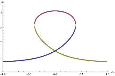
Figure 1: Effect of the beam tilts removal on the horizontal projected emittance $\varepsilon_{x}$ as a functions of the $r_{56}$ coefficient.

The effect of the zeroing of the beam tilts in the matrix (336) on projected emittances is presented at figures 1 and 2, where the resulting emittances are shown for all possible real solutions of the equation (340). One has to compare these emittances with the emittances $\varepsilon_{x}=1$, $\varepsilon_{\sigma}=6$ of the original beam matrix (336) and with the emittances $\varepsilon_{x}\approx 0.577$, $\varepsilon_{\sigma}\approx 5.354$ which can be obtained after removal of the beam dispersions.

V.4 Conditions for complete transverse to longitudinal decoupling

The example considered in the previous subsection tells us that zeroing of the beam tilts does not necessarily implies reduction of the transverse projected emittances. The situation, of course, will be different if zeroing of the beam tilts will simultaneously remove the beam dispersions, i.e. if the longitudinal and transverse degrees of freedom in the beam matrix $\Sigma$ will be decoupled from each other at the correction system exit. The necessary and sufficient conditions for the complete transverse to longitudinal decoupling can be obtained by the requirement that the solution for the lattice dispersions (190) which removes the beam dispersions also zeros the beam tilts, and substituting (190) into the equations (316) and (325) we obtain (without big surprise) again the equations (300), which were derived as conditions for the simultaneous minimization of all projected emittances.

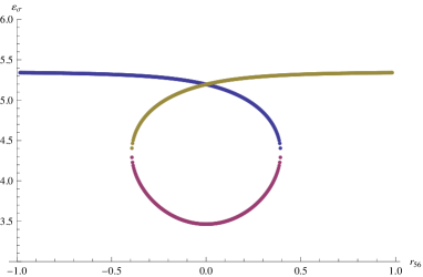
Figure 2: Effect of the beam tilts removal on the longitudinal projected emittance $\varepsilon_{\sigma}$ as a functions of the $r_{56}$ coefficient.

The most difficult question, for which we do not have any good answers yet, is the question of the physical interpretation of the conditions (300). It is clear, for example, that if the distortions to the initially uncoupled beam matrix $\Sigma$ were produced by a magnetostatic system, then the decoupling also can be done by a magnetostatic system, but how such beam matrices can be described more intuitively and what are the other possibilities? Currently, as more physical example in the comparison with the conditions (300) description, we only can state that all beam matrices with equal eigenemittances (definition and properties of eigenemittances can be found in MomInv_4 ; MyEE ) always can be decoupled by a magnetostatic system. It follows from the observation that the conditions (300) are equivalent to the property of the matrix $(\Sigma J_{6})^{2}$ to have zeros in the positions

$$(\Sigma J_{6})^{2}=\left(\begin{array}[]{cccccc}*&*&*&*&0&*\\ &*&*&*&0&*\\ &*&*&*&0&*\\ &*&*&*&0&*\\ &*&*&*&*&*\\ 0&0&0&0&*&*\end{array}\right),$$ (349)

and from the fact proven in My02 that if the matrix $\Sigma$ has all eigenemittances equal to each other, then the matrix $(\Sigma J_{6})^{2}$ is a diagonal matrix.

V.5 Illustrative example

We have seen that if in the beam matrix $\Sigma$ there are nonzero correlations between energy of particles and their transverse positions and momenta, then the values of the transverse projected emittances can be reduced, but how these reduced emittances are related to the emittances of the particle beam before it was damaged by the CSR wake (or by some other effects) remains, of course, completely unclear. So, let us consider an example which would give at least some insights into this problem.

Let us assume that we have in the beginning a particle beam with the beam matrix $\Sigma$ in which all degrees of freedom are decoupled from each other

$$\Sigma=\left(\begin{array}[]{cccccc}\langle x^{2}\rangle&\langle xp_{x}\rangle&0&0&0&0\\ \langle xp_{x}\rangle&\langle p_{x}^{2}\rangle&0&0&0&0\\ 0&0&\langle y^{2}\rangle&\langle yp_{y}\rangle&0&0\\ 0&0&\langle yp_{y}\rangle&\langle p_{y}^{2}\rangle&0&0\\ 0&0&0&0&\langle\sigma^{2}\rangle&\langle\sigma\varepsilon\rangle\\ 0&0&0&0&\langle\sigma\varepsilon\rangle&\langle\varepsilon^{2}\rangle\end{array}\right),$$ (356)

and then this beam passes through a beamline described by the matrix

$$T=\left(\begin{array}[]{cccccc}1&0&0&0&0&0\\ 0&1&0&0&a&0\\ 0&0&1&0&0&0\\ 0&0&0&1&0&0\\ 0&0&0&0&1&0\\ a&0&0&0&b&1\end{array}\right),\quad a\neq 0.$$ (363)

Our choice of the matrix $T$ as a source of the growth of the projected emittances and also as a source of the transverse to longitudinal coupling is motivated by the following reasons: The matrix $T$, from one side, is symplectic and therefore all changes which it introduces are reversible, but it is not the matrix of a magnetostatic system and it is interesting to see up to what extend the original projected emittances of the matrix $(\ref{Form1960})$ can be recovered afterwards by a magnetostatic correction system. From the other side, this matrix, similar to the wake field action, provides transverse kick and energy loss to the particle depending on its longitudinal position within the bunch. Note that if parameters $a$ and $b$ in this matrix are related to each other in some special way, then the matrix $T$ becomes equal to the matrix of the thick-lens horizontally deflecting cavity when it is sandwiched between two drifts of equal negative lengths (see, for example, CornEmma ).

The passage of the beam matrix (356) through the system described by the matrix $T$ gives equal increase of horizontal and longitudinal projected emittances (the vertical degree of freedom remains decoupled from the others and is ignored in the following considerations)

$$\varepsilon_{x}^{2}\,\leftarrow\,\varepsilon_{x}^{2}\,+\,a^{2}\,\langle x^{2}\rangle\,\langle\sigma^{2}\rangle,$$ (364)

$$\varepsilon_{\sigma}^{2}\,\leftarrow\,\varepsilon_{\sigma}^{2}\,+\,a^{2}\,\langle x^{2}\rangle\,\langle\sigma^{2}\rangle,$$ (365)

and generates horizontal to longitudinal coupling terms (beam dispersions and beam tilts)

$$\langle x\varepsilon\rangle\,\leftarrow\,a\,\langle x^{2}\rangle,$$ (366)

$$\langle p_{x}\varepsilon\rangle\,\leftarrow\,a\,\left(\langle xp_{x}\rangle\,+\,\langle\sigma\varepsilon\rangle\,+\,b\,\langle\sigma^{2}\rangle\right),$$ (367)

$$\langle x\sigma\rangle\,\leftarrow\,0,$$ (368)

$$\langle p_{x}\sigma\rangle\,\leftarrow\,a\,\langle\sigma^{2}\rangle.$$ (369)

The rms bunch length squared $\langle\sigma^{2}\rangle$ is conserved, but the rms energy spread evolves according to the formula

$$\langle\varepsilon^{2}\rangle\,\leftarrow\,\mbox{\ae},$$ (370)

where

$$\mbox{\ae}=\langle\varepsilon^{2}\rangle\,+\,a^{2}\,\langle x^{2}\rangle\,+\,2\,b\,\langle\sigma\varepsilon\rangle\,+\,b^{2}\,\langle\sigma^{2}\rangle\,>\,0,$$ (371)

and the beam energy chirp also experiences some change

$$\langle\sigma\varepsilon\rangle\,\leftarrow\,\langle\sigma\varepsilon\rangle\,+\,b\,\langle\sigma^{2}\rangle.$$ (372)

The equations (300), when applied to the matrix $T\Sigma T^{\top}$, are reduced to the single relation

$$\varepsilon_{x}\,=\,\varepsilon_{\sigma}$$ (373)

among the elements of the matrix $\Sigma$. It means that both projected emittances can be recovered by a magnetostatic correction (and also the beam matrix can be decoupled) if and only if horizontal and longitudinal projected emittances were equal in the beginning before the passage through the system described by the matrix $T$. But let us see what can be done if they were not. So, as the next step, let the beam pass through the dispersive part of the downstream correction system and, because we would like to express the final results using the elements of the original matrix (356), let us consider the transformation

$$\Sigma\leftarrow(R_{2}T)\,\Sigma\,(R_{2}T)^{\top},$$ (374)

instead of the transformation (62).

The formulas (85) and (89) for the transport of the horizontal and longitudinal projected emittances, when adapted to the transport equation (374), can be rewritten as follows:

$$\varepsilon_{x}^{2}\,\leftarrow\,\varepsilon_{x}^{2}\,+\,\Psi_{F}(r_{51}^{x}-r_{51},\,r_{52}^{x}-r_{52})\,-\,\Psi_{F}^{x},$$ (375)

where

$$r_{51}^{x}\,=\,a\,\frac{\langle xp_{x}\rangle+\langle\sigma\varepsilon\rangle+b\,\langle\sigma^{2}\rangle}{\mbox{\ae}},$$ (376)

$$r_{52}^{x}\,=\,-a\,\frac{\langle x^{2}\rangle}{\mbox{\ae}},$$ (377)

and

$$\Psi_{F}^{x}\,=\,-\frac{a^{2}\langle x^{2}\rangle}{\mbox{\ae}}\,\left(\varepsilon_{\sigma}^{2}\,-\,\varepsilon_{x}^{2}\right).$$ (378)

$$\varepsilon_{\sigma}^{2}\,\leftarrow\,\varepsilon_{\sigma}^{2}\,+\,\Psi_{F}(r_{51}^{\sigma}-r_{51},\,r_{52}^{\sigma}-r_{52})\,-\,\Psi_{F}^{\sigma},$$ (379)

where

$$r_{51}^{\sigma}\,=\,a\,\frac{\left(\langle\sigma\varepsilon\rangle+b\,\langle\sigma^{2}\rangle\right)\,\varepsilon_{x}^{2}\,+\,\langle xp_{x}\rangle\,\varepsilon_{\sigma}^{2}}{\varkappa},$$ (380)

$$r_{52}^{\sigma}=-a\,\frac{\langle x^{2}\rangle\,\varepsilon_{\sigma}^{2}}{\varkappa},$$ (381)

$$\Psi_{F}^{\sigma}\,=\,\frac{a^{2}\langle x^{2}\rangle\,\varepsilon_{\sigma}^{2}}{\varkappa}\,\left(\varepsilon_{\sigma}^{2}\,-\,\varepsilon_{x}^{2}\right),$$ (382)

and

$$\varkappa\,=\,a^{2}\langle x^{2}\rangle\left(\varepsilon_{\sigma}^{2}\,-\,\varepsilon_{x}^{2}\right)+\mbox{\ae}\,\varepsilon_{x}^{2}\,>\,0.$$ (383)

Note that in the above formulas $\Psi_{F}$ is a positive definite quadratic form in two variables obtained from the quadratic form $\Psi_{A}$, and the exact expression for the $2\times 2$ matrix associated with the quadratic form $\Psi_{F}$ is unimportant for the further consideration.

From the equation (375) one sees that the original horizontal projected emittance $\varepsilon_{x}$ can be recovered if and only if

$$\Psi_{F}^{x}\,\geq\,0\quad\Leftrightarrow\quad\varepsilon_{x}\,\geq\,\varepsilon_{\sigma},$$ (384)

and the condition for the recovering of $\varepsilon_{\sigma}$ coming from the equation (379) is

$$\Psi_{F}^{\sigma}\,\geq\,0\quad\Leftrightarrow\quad\varepsilon_{\sigma}\,\geq\,\varepsilon_{x}.$$ (385)

So, as one sees, if $\varepsilon_{x}\neq\varepsilon_{\sigma}$, then only the larger of the two can be repaired and even can be further reduced, but only on expense of the increase of the other. Nevertheless, even if the horizontal (or longitudinal) projected emittance cannot be recovered to its original value, the distorted value (364) (or (365)) always can be reduced, as follows from the theory developed in this paper.

Let us now consider three extreme cases: solution for the lattice dispersions which minimizes $\varepsilon_{x}$, solution which minimizes $\varepsilon_{\sigma}$ and solution which zeros beam tilts. Even before making any calculations, one can state that in all these three cases the sum

$$\varepsilon_{x}^{2}\,+\,\varepsilon_{\sigma}^{2}$$ (386)

will be conserved, which follows from the preservation of the Lysenko invariant (254) and the fact that all these solutions make the vector of the beam dispersions and the vector of the beam tilts linearly dependent at the correction system exit. Note also that due to the conservation of the sum (386) and due to the extremum properties of the solutions which minimize projected emittances, any solution which zeros beam tilts will give the final value of the transverse projected emittance which must lie between the values given by the solution which zeros beam dispersions and the solution which minimizes longitudinal projected emittance.

The setting of the lattice dispersions to the values $r_{51}=r_{51}^{x}$ and $r_{52}=r_{52}^{x}$ which minimize the horizontal projected emittance $\varepsilon_{x}$ gives us

$$\varepsilon_{x}^{2}\,\leftarrow\,\varepsilon_{x}^{2}\,+\,\frac{a^{2}\langle x^{2}\rangle}{\mbox{\ae}}\,\left(\varepsilon_{\sigma}^{2}\,-\,\varepsilon_{x}^{2}\right),$$ (387)

$$\varepsilon_{\sigma}^{2}\,\leftarrow\,\varepsilon_{\sigma}^{2}\,-\,\frac{a^{2}\langle x^{2}\rangle}{\mbox{\ae}}\,\left(\varepsilon_{\sigma}^{2}\,-\,\varepsilon_{x}^{2}\right),$$ (388)

and minimization of the longitudinal projected emittance $\varepsilon_{\sigma}$ by the setting $r_{51}=r_{51}^{\sigma}$ and $r_{52}=r_{52}^{\sigma}$ produces

$$\varepsilon_{x}^{2}\,\leftarrow\,\varepsilon_{x}^{2}\,+\,\frac{a^{2}\langle x^{2}\rangle\,\varepsilon_{\sigma}^{2}}{\varkappa}\,\left(\varepsilon_{\sigma}^{2}\,-\,\varepsilon_{x}^{2}\right),$$ (389)

$$\varepsilon_{\sigma}^{2}\,\leftarrow\,\varepsilon_{\sigma}^{2}\,-\,\frac{a^{2}\langle x^{2}\rangle\,\varepsilon_{\sigma}^{2}}{\varkappa}\,\left(\varepsilon_{\sigma}^{2}\,-\,\varepsilon_{x}^{2}\right).$$ (390)

Unfortunately, it is practically impossible to find the general solutions for the lattice dispersions which are required for the zeroing of the beam tilts in the analytical form, and we will give it only for the partial case when $r_{56}=b=0$. With this assumption the solution for the zeroing of the beam tilts is unique and is given by the following formulas

$$r_{51}\,=\,\frac{a\langle\sigma^{2}\rangle\left(\langle xp_{x}\rangle+\langle\sigma\varepsilon\rangle\right)}{\kappa},$$ (391)

$$r_{52}\,=\,-\frac{a\langle x^{2}\rangle\langle\sigma^{2}\rangle}{\kappa},$$ (392)

where

$$\kappa\,=\,\varepsilon_{x}^{2}\,+\,a^{2}\langle x^{2}\rangle\langle\sigma^{2}\rangle\,+\,\langle\sigma\varepsilon\rangle^{2},$$ (393)

and the resulting formulas for the transport of the projected emittances are

$$\varepsilon_{x}^{2}\,\leftarrow\,\varepsilon_{x}^{2}\,+\,\frac{a^{2}\langle x^{2}\rangle\langle\sigma^{2}\rangle}{\kappa}\,\left(\varepsilon_{\sigma}^{2}\,-\,\varepsilon_{x}^{2}\right),$$ (394)

$$\varepsilon_{\sigma}^{2}\,\leftarrow\,\varepsilon_{\sigma}^{2}\,-\,\frac{a^{2}\langle x^{2}\rangle\langle\sigma^{2}\rangle}{\kappa}\,\left(\varepsilon_{\sigma}^{2}\,-\,\varepsilon_{x}^{2}\right).$$ (395)

One can check that while for $a\neq 0$ the result of (387) is always smaller than the result of (364) (as expected), the values produced by the formulas (389) and (394) for $\varepsilon_{x}\neq\varepsilon_{\sigma}$ can reduce the distorted emittance (364) only under specific conditions.

- (1) A.Loulergue and A.Mosnier, “A simple S-chicane for the final bunch compressor of TTF FEL”, Proceedings of EPAC 2000, Vienna, Austria, June 26-30, 2000, WEP4B01.
- (2) M.Dohlus and T.Limberg “Impact of optics on CSR-related emittance growth in bunch compressor chicanes”, Proceedings of PAC 2005, Knoxville, Tennessee, USA, May 16-20, 2005, TPAT006.
- (3) S.Di Mitri et all, “Cancellation of coherent synchrotron radiation kicks with optics balance”, Phys. Rev. Letters 110, 014801 (2013).
- (4) Y.Jing,Y.Hao, and V.N.Litvinenko, “Compensating effect of the coherent synchrotron radiation in bunch compressors”, Phys. Rev. ST Accel. Beams 16, 060704 (2013).
- (5) C.Mitchell, J.Qiang, and P.Emma, “Longitudinal pulse shaping for the suppression of coherent synchrotron radiation-induced emittance growth”, Phys. Rev. ST Accel. Beams 16, 060703 (2013)
- (6) V.Balandin, W.Decking, and N.Golubeva, “Interaction between beam dispersions and lattice dispersions”, Unpublished Note, September 2009.
- (7) V.Ayvazian et al., “First operation of a free-electron laser generating GW power radiation at 32 nm wavelength”, Eur. Phys. J. D 37 (2006) 297.
- (8) W.Ackermann et al., “Operation of a free-electron laser from the extreme ultraviolet to the water window”, Nature Photonics 1 (2007) 336.
- (9) M.W.Guetg, B.Beutner, E.Prat, and S.Reiche “Dispersion based beam tilt correction”, Proceedings of FEL 2013, New York, NY, USA, August 25-30, 2013, TUPSO24.
- (10) H.Mais and G.Ripken, “Theory of coupled synchro-betatron oscillations (I)”, Internal Report, DESY M-82-05, 1982.
- (11) V.Balandin and N.Golubeva, “Hamiltonian methods for the study of polarized proton beam dynamics in accelerators and storage rings”, DESY 98-016, February 1998 (arXiv: physics/9903032).
- (12) R.A.Horn and C.R.Johnson, “Matrix analysis”, University Press, Cambridge, 1990.
- (13) W.P.Lysenko and M.Overley, “Moment invariants for particle beams”, AIP Conf. Proc., 177 (1988), no. 1, 323-335.
- (14) W.P.Lysenko, “The moment approach to high-order accelerator beam optics”, Nucl. Instr. Meth. A363 (1995), 90-99.
- (15) F.Neri and G.Rangarajan, “Kinematic moment invariants for linear Hamiltonian systems”, Phys. Rev. Letters 64, 1073 (1990).
- (16) V.Balandin, W.Decking, and N.Golubeva, “Relations between projected emittances and eigenemittances”, Proceedings of IPAC 2013, Shanghai, China, May 12-17 May, 2013, TUPWO012.
- (17) V.Balandin, R.Brinkmann, W.Decking, and N.Golubeva, “Twiss parameters of coupled particle beams with equal eigenemittances”, Proceedings of IPAC 2012, New Orleans, Louisiana, USA, May 20-25, 2012, TUPPC008.
- (18) M.Cornacchia and P.Emma, “Transverse to longitudinal emittance exchange”, Phys. Rev. ST Accel. Beams 5, 084001 (2002).