Antiferromagnetic Topological Superconductor
and Electrically Controllable Majorana Fermions

Abstract

We investigate the realization of a topological superconductor in a generic bucked honeycomb system equipped with four types of mass-generating terms, where the superconductor gap is introduced by attaching the honeycomb system to an $s$-wave superconductor. Constructing the topological phase diagram, we show that Majorana modes are formed in the phase boundary. In particular, we analyze the honeycomb system with antiferromagnetic order in the presence of perpendicular electric field $E_{z}$. It becomes topological for $|E_{z}|>E_{z}^{\text{cr}}$ and trivial for $|E_{z}|<E_{z}^{\text{cr}}$, with $E_{z}^{\text{cr}}$ a certain critical field. It is possible to create a topological spot in a trivial superconductor by controlling applied electric field. One Majorana zero-energy bound state appears at the phase boundary. We can arbitrarily control the position of the Majorana fermion by moving the spot of applied electric field, which will be made possible by a scanning tunneling microscope probe.

Topological superconductor and Majorana fermion are among the hottest topics in condensed matter physicsAlicea ; Beenakker ; Flen ; Qi . Majorana fermions will be a key player of future quantum computationsIvanov ; Nayak . The anti-particle of a Majorana fermion is itself. Zero-energy states of a superconductor are necessarily Majorana modes based on the particle-hole symmetry. One dimensional $p$-wave topological superconductorKitaev ; Alicea ; Flen ; Beenakker and two-dimensional ($p$+$ip$)-wave topological superconductor are fundamental models to realize themRead ; Ivanov . Another promising candidate would be to utilize the quantum anomalous Hall (QAH) insulator with a proximity-coupled $s$-wave normal superconductorQiQAH . It is a time-reversal breaking topological superconductorSchnyder with class D.

In this paper, we investigate topological superconductivity in a generic honeycomb system in proximity to an $s$-wave superconductor. Honeycomb monolayer systems have provided us with an interesting playground of two dimensional topological insulators. In particular, the buckled honeycomb system exhibits various topological phases such as the quantum spin Hall (QSH) insulator, the QAH insulator and the spin-polarized QAH (SP-QAH) insulatorEzawaPhoto ; Ezawa2Ferro depending on the four mass parameters. The driving forces are the Kane-Mele spin-orbit interactionKaneMele with coupling parameter $\lambda_{\text{SO}}$, the staggered potential with $\lambda_{V}$, the antiferromagnetic order with $\lambda_{\text{SX}}$ and the Haldane termKitagawa ; EzawaPhoto with $\lambda_{\text{H}}$, generating the mass $\Delta$ to the Dirac fermions intrinsic to the honeycomb system. The Chern number is calculated to be $\frac{1}{2}$sgn$(\Delta)$ for each Dirac cone, which depends on these parameters. The topological phase diagram is constructed in the ($\lambda_{\text{SO}},\lambda_{V},\lambda_{\text{SX}},\lambda_{\text{H}}$) space. There are important observations. First, it is possible to control the Dirac mass $\Delta$ locally by controlling the external forces. The easiest one is the control of the staggered potential by changing the applied electric fieldEzawaNJP . The phase boundary is given by the condition $\Delta=0$. Hence we are able to accommodate two different topological phases in a single honeycomb systemEzawaNJP . Gapless Dirac modes ($\Delta=0$) are generated along a phase boundary, as is consistent with the bulk-edge correspondence. They are helical, chiral or spin-polarized modes emerging in the edge of the QSH, QAH and SP-QAH insulators, respectively.

The honeycomb system is made superconducting in proximity to an $s$-wave superconductor. The natural question is whether a topological insulator turns into a topological superconductor. We construct the topological phase diagram in the ($\lambda_{\text{SO}},\lambda_{V},\lambda_{\text{SX}},\lambda_{\text{H}},\Delta_{\text{SC}}$) space, where $\Delta_{\text{SC}}$ is the superconducting gap. Our results read as follows: The time-reversal symmetry is broken in all topologically non-trivial superconductors constructed in this system. Gapless Majorana modes emerge in the phase boundary. Spin-polarized and chiral edge modes yield one and two Majorana edge modes, respectively. Helical modes are gapped. Consequently, by controlling external forces locally, we are able to generate Majorana bound states in the phase boundary of a topological superconductor created within a trivial superconductor sheet.

A special role is played by the SP-QAH insulatorEzawaPhoto ; Ezawa2Ferro since its Chern number is one. It is an antiferromagnetic topological insulator. The antiferromagnet order in honeycomb system would be naturally realized in transition metal oxidesHu . We study the antiferromagnetic topological superconductor obtained by the proximity effect. We apply electric field locally to the sample. For instance, let us apply it in such a way that $\lambda_{V}>\lambda_{V}^{\text{cr}}$ for $r<r_{0}$ and $\lambda_{V}<\lambda_{V}^{\text{cr}}$ for $r>r_{0}$ in the polar coordinate with $\lambda_{V}^{\text{cr}}$ being a certain critical potential. One Majorana fermion is induced at the phase boundary $r=r_{0}$. We may arbitrarily control its position by moving the region of electric field, which will be experimentally feasible by a scanning tunneling microscope (STM) probe.

Honeycomb system: A generic buckled honeycomb system is described by the four-band tight-binding modelKaneMele ; LiuPRB ; Ezawa2Ferro ,

$$H_{0}= -t\sum_{\left\langle i,j\right\rangle\alpha}c_{i\alpha}^{\dagger}c_{j\alpha}+i\frac{\lambda_{\text{SO}}}{3\sqrt{3}}\sum_{\left\langle\!\left\langle i,j\right\rangle\!\right\rangle\alpha\beta}\nu_{ij}c_{i\alpha}^{\dagger}\sigma_{\alpha\beta}^{z}c_{j\beta}$$

$$-\lambda_{V}\sum_{i\alpha}\mu_{i}c_{i\alpha}^{\dagger}c_{i\alpha}+\lambda_{\text{SX}}\sum_{i\alpha}\mu_{i}c_{i\alpha}^{\dagger}\sigma_{\alpha\alpha}^{z}c_{i\alpha}$$

$$+i\frac{\lambda_{\text{H}}}{3\sqrt{3}}\sum_{\left\langle\!\left\langle i,j\right\rangle\!\right\rangle\alpha\beta}\nu_{ij}c_{i\alpha}^{\dagger}c_{j\beta},$$ (1)

where $c_{i\alpha}^{\dagger}$ creates an electron with spin polarization $\alpha$ at site $i$, and $\left\langle i,j\right\rangle/\left\langle\!\left\langle i,j\right\rangle\!\right\rangle$ run over all the nearest/next-nearest neighbor hopping sites. The first term represents the nearest-neighbor hopping with the transfer energy $t$. The second term represents the spin-orbit couplingKaneMele with $\lambda_{\text{SO}}$, where $\nu_{ij}=+1$ if the next-nearest-neighboring hopping is anticlockwise and $\nu_{ij}=-1$ if it is clockwise with respect to the positive $z$ axis. The third term is the staggered sublattice potentialEzawaNJP with $\lambda_{V}$, where $\mu_{i}$ takes $1$ ($-1$) for $A$ ($B$) sites. The staggered term may exist intrinsically or induced by applying electric field $E_{z}$, $\lambda_{V}=\ell E_{z}$. The forth term represents the antiferromagnetic exchange magnetizationEzawa2Ferro ; Feng with $\lambda_{\text{SX}}$. The fifth term is the Haldane termHaldane with $\lambda_{\text{H}}$, which will be introduced by applying photo-irradiationKitagawa ; EzawaPhoto .

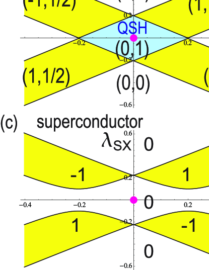
Figure 1: (Color online) Topological phase diagrams in (a) the $(\lambda_{V},\lambda_{\text{SX}},\Delta_{\text{SC}})$ space and (a’) the $(\lambda_{V},\lambda_{\text{H}},\Delta_{\text{SC}})$ space, where we have taken $\lambda_{\text{SO}}=0.2t$. Phase diagrams for topological insulator in (b) the $(\lambda_{V},\lambda_{\text{SX}})$ space and (b’) the $(\lambda_{V},\lambda_{\text{H}})$ space. Each phase is indexed by the set $(C,C_{\text{spin}})$ of the Chern and spin-Chern numbers. Phase diagrams for topological superconductor in (c) the $(\lambda_{V},\lambda_{\text{SX}})$ space and (c’) the $(\lambda_{V},\lambda_{\text{H}})$ space, where we have taken $\Delta_{\text{SC}}=0.1t$. Each phase is indexed by the Chern number $C$. Tree red dots in (b,b’) [(c,c’)] show points where the band structure of nanoribbons are calculated and shown in Fig.2(a,b,c) [(a’,b’,c’)].

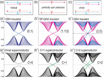
Figure 2: (Color online) Zero-energy edge modes in a nanoribbon for (a) the QSH insulator, (b) the SP-QAH insulator and (c) the QAH insulator. Up (down) arrow indicates up (down) spin, while solid (dotted) line indicates right (left) edge mode. Band structures of these nanoribbons are given in (a’), (b’) and (c’). Majorana modes emerge along a phase boundary between topological and trivial superconductors. There appear (a") zero, (b") one and (c") two Majorana modes in superconductor nanoribbons as indicated by green curves.

Topological insulator: The physics of electrons near the Fermi energy is described by Dirac electrons near the $K$ and $K^{\prime}$ points, to which we also refer as the $K_{\eta}$ points with $\eta=\pm$. The effective Dirac Hamiltonian around the $K_{\eta}$ point in the momentum space readsEzawaAQHE

$$H_{\eta}= \hbar v_{\text{F}}\left(\eta k_{x}\tau_{x}+k_{y}\tau_{y}\right)$$

$$+\lambda_{\text{SO}}\sigma_{z}\eta\tau_{z}-\lambda_{V}\tau_{z}+\lambda_{\text{SX}}\sigma_{z}\tau_{z}+\lambda_{\text{H}}\eta\tau_{z},$$ (2)

where $\sigma_{a}$ and $\tau_{a}$ are the Pauli matrices of the spin and the sublattice pseudospin, respectively and $v_{\text{F}}=\frac{\sqrt{3}}{2\hbar}at$ is the Fermi velocity. The coefficient of $\tau_{z}$ is the mass of Dirac fermions in the Hamiltonian, which is composed of four terms,

$$\Delta_{s_{z}}^{\eta}=\eta s_{z}\lambda_{\text{SO}}-\lambda_{V}+s_{z}\lambda_{\text{SX}}+\eta\lambda_{\text{H}},$$ (3)

with $s_{z}=\pm$ for the spin direction. The energy spectrum forms a Dirac cone at the $K_{\eta}$ point with the band gap $2|\Delta_{s_{z}}^{\eta}|$.

The Chern number is obtained for each Dirac cone by calculating the Berry connection, which is given by $C_{s_{z}}^{\eta}=\frac{1}{2}$sgn$(\Delta_{s_{z}}^{\eta})$. The total Chern number is $C=C_{\uparrow}^{+}+C_{\uparrow}^{-}+C_{\uparrow}^{+}+C_{\uparrow}^{-}$, while the spin-Chern number is $C_{\text{spin}}=C_{\uparrow}^{+}+C_{\uparrow}^{-}-C_{\downarrow}^{+}-C_{\downarrow}^{-}$. The topological phase diagram is constructed in the $(\lambda_{\text{SO}},\lambda_{V},\lambda_{\text{SX}},\lambda_{\text{H}})$ space by calculating $(C,C_{\text{spin}})$ at each point. The condition of topological insulator is $(C,C_{\text{spin}})\neq(0,0)$. In particular, the state with $(0,1)$, $(2,0)$ and $(1,1/2)$ are the QSH, QAH and SP-QAH insulators.

The phase boundary is given by $\Delta_{s_{z}}^{\eta}=0$. We give typical examples of the phase diagram in the $(\lambda_{V},\lambda_{\text{SX}})$ and $(\lambda_{V},\lambda_{\text{H}})$ spaces in Figs.1(b) and (b’), respectively. The band structures and edge modes are illustrated for typical topological insulator nanoribbons in Fig.2(a), (b), (c) and (a’), (b’) and (c’).

Topological superconductor: A topological superconductor is obtained from a topological insulator due to the proximity effectFuKane by attaching an $s$-wave superconductor to it. Indeed, Cooper pairs are formedGapClose between up and down spins at the same site of the honeycomb system (1). The resultant BCS Hamiltonian reads

$$H_{\text{BCS}}=H_{0}+\sum_{\tau=A,B}\Delta_{\text{SC}}c_{\tau\uparrow}^{\dagger}\left(i\right)c_{\tau\downarrow}^{\dagger}\left(i\right)+\Delta_{\text{SC}}^{\ast}c_{\tau\downarrow}\left(i\right)c_{\tau\uparrow}\left(i\right),$$ (4)

where $H_{0}$ is given by (1) and $\Delta_{\text{SC}}$ is the superconducting gap. It readsGapClose $H_{\text{BCS}}=H_{K}+H_{K^{\prime}}+H_{\text{SC}}$ with

$$H_{\text{SC}}= \sum_{\tau=A,B}[\Delta_{\text{SC}}c_{\tau\uparrow}^{K\dagger}\left(k\right)c_{\tau\downarrow}^{K^{\prime}\dagger}\left(-k\right)+\Delta_{\text{SC}}c_{\tau\uparrow}^{K^{\prime}\dagger}\left(k\right)c_{\tau\downarrow}^{K\dagger}\left(-k\right)]$$

$$+\text{h.c.}$$ (5)

in the momentum representation. A finite gap present in a superconducting state allows us to evaluate the Chern number of the state to determine whether it is a topological state. Alternatively we may examine the emergence of gapless edge modes by calculating the band structure of a nanoribbon with zigzag edge geometry based on this Hamiltonian. The emergence of gapless edge modes presents a best signal of a nontrivial topological structure in the system based on the bulk-edge correspondence: See Fig.2(a"), (b") and (c").

The BCS Hamiltonian is rewritten into the BdG Hamiltonian,

$$H_{\text{BdG}}=\left(\begin{array}[]{cc}H_{K}\left(k\right)&H_{\Delta}\\ H_{\Delta}^{\dagger}&-H_{K^{\prime}}^{\ast}\left(-k\right)\end{array}\right),$$ (6)

by introducing the Nambu representation for the basis vector, i.e., $\Psi=\left\{\psi_{A\uparrow}^{K},\psi_{B\uparrow}^{K},\psi_{A\downarrow}^{K},\psi_{B\downarrow}^{K},\psi_{A\uparrow}^{K^{\prime}\dagger},\psi_{B\uparrow}^{K^{\prime}\dagger},\psi_{A\downarrow}^{K^{\prime}\dagger},\psi_{B\downarrow}^{K^{\prime}\dagger}\right\}^{t}$.

Diagonalizing the BdG Hamiltonian, we obtain the energy spectrum. It consists of eight levels with the eigenvalues

$$E_{\text{BdG}}^{\alpha,\beta}\left(k\right)=\pm\sqrt{\left(\hbar v_{\text{F}}k\right)^{2}+\left(E_{0}^{\alpha,\beta}\right)^{2}}$$ (7)

with

$$E_{0}^{\alpha,\beta}=\sqrt{\left(\left(\lambda_{\text{SO}}-\alpha\lambda_{V}\right)^{2}+\Delta_{\text{SC}}^{2}\right)}+\beta\left(\lambda_{\text{H}}+\alpha\lambda_{\text{SX}}\right),$$ (8)

where $\alpha$ and $\beta$ takes $\pm 1$. The gap closes ($E_{0}^{\alpha,\beta}=0$) at

$$\left(\lambda_{\text{H}}+\alpha\lambda_{\text{SX}}\right)^{2}=\left(\lambda_{\text{SO}}-\alpha\lambda_{V}\right)^{2}+\Delta_{\text{SC}}^{2}.$$ (9)

Though the original Hamiltonian is an $8\times 8$ matrix, we may decompose it into 4 independent $2\times 2$ Hamiltonians by the following procedure: First we diagonalize the Hamiltonian at the $K$ and $K^{\prime}$ points by the unitary matrix $U$, $U^{-1}H_{\text{BdG}}\left(0\right)U=$diag.$\left\{E_{\text{BdG}}^{\alpha,\beta}\left(0\right)\right\}$. Then we calculate $U^{-1}H_{\text{BdG}}\left(k\right)U$. The resultant matrix is constituted of the 4 blocks of $2\times 2$ matrix. As a result, corresponding to $\alpha,\beta=\pm 1$, we obtain four sets of the 2-band theories,

$$H_{U}\left(k\right)=\left(\begin{array}[]{cc}\beta E_{0}^{\alpha,\beta}&\hbar v_{\text{F}}k_{-}\\ \hbar v_{\text{F}}k_{+}&-\beta E_{0}^{\alpha,\beta}\end{array}\right).$$ (10)

This Hamiltonian reproduces the energy spectrum (7). We may interpret $\beta E_{0}^{\alpha,\beta}$ as the modified Dirac mass due to the BCS condensation.

It is straightforward to calculate the Chern number of the superconducting honeycomb system $H_{\text{BdG}}$. It is determined by the sign of the modified Dirac massDiamag ,

$$C=\frac{1}{2}\sum_{\alpha,\beta=\pm 1}\text{sgn}\left(\beta E_{0}^{\alpha,\beta}\right).$$ (11)

The condition of the emergence of a topological superconductivity is $C\neq 0$. Note that it is zero when the time-reversal symmetry is present. In order to obtain a non-zero Chern number, $\lambda_{\text{SX}}$ or $\lambda_{\text{H}}$ must be nonzero. It should be noticed that the spin-Chern number is no longer defined due to the BCS condensation of the up-spin and down-spin electrons.

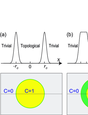
Figure 3: (Color online) Illustration of a Majorana zero-energy state emerging in antiferromagnetic superconductor. By applying electric field $E_{z}$ locally, we may create a topological spot ($C=1$) in a trivial superconductor ($C=0$). There appears one zero-energy Majorana state in the phase boundary. (a) The phase boundary is one dimensional in the case of (15). (b) It may be two dimensional when we set $E_{0}^{\alpha,\beta}(r)=0$ for a finite domain of $r$.

The topological phase diagram is easily constructed in the $(\lambda_{\text{SO}},\lambda_{V},\lambda_{\text{SX}},\lambda_{\text{H}},\Delta_{\text{SC}})$ space. The phase boundaries are given by (9). The Chern number is determined from (11). We show typical examples of the phase diagram in the $(\lambda_{V},\lambda_{\text{SX}})$ and $(\lambda_{V},\lambda_{\text{H}})$ spaces in Fig.1(c) and (c’). We also show the band structure of a nanoribbons at a typical point in each phase in Fig.2(a"), (b") and (c"): There appear no, one and two zero-energy edge modes, respectively.

Zero-energy Majorana bound states: The zero-energy edge modes are Majorana bound states due to the electron-hole symmetry. For definiteness we consider a disk region in a honeycomb sheet, as illustrated in Fig.3. We may tune parameters $\lambda_{\text{SO}}$, $\lambda_{V}$, $\lambda_{\text{SX}}$, $\lambda_{\text{H}}$ and $\Delta_{\text{SC}}$ to become space-dependent so that the inner region has a different Chern number from the outer region. There appears gapless edge modes at the phase boundary. The Majorana bound states are obtained analytically by solving the BdG equation.

We take the polar coordinate $\left(r,\theta\right)$. By inserting $k_{\pm}=e^{\pm i\theta}(-i\partial_{r}\pm\frac{1}{r}\partial_{\theta})$ into (10) and setting $\Psi=\{\phi_{A}\left(r\right)e^{in\theta},\phi_{B}\left(r\right)e^{i(n+1)\theta}\}^{t}$ for the wave function, the Hamiltonian is written as

$$H_{U}=\left(\begin{array}[]{cc}E_{0}^{\alpha,\beta}\left(r\right)&\hbar v_{\text{F}}(-i\partial_{r}-\frac{i(n+1)}{r})\\ \hbar v_{\text{F}}(-i\partial_{r}+\frac{in}{r})&-E_{0}^{\alpha,\beta}\left(r\right)\end{array}\right),$$ (12)

where $E_{0}^{\alpha,\beta}\left(r\right)$ is the inhomogeneous mass (8) with space-dependent parameters $\lambda_{\text{SO}}$, $\lambda_{V}$, $\lambda_{\text{SX}}$, $\lambda_{\text{H}}$ and $\Delta_{\text{SC}}$. By assuming $\phi_{B}\left(r\right)=\pm i\phi_{A}\left(r\right)$ for $n=-1/2$, the coupled equation $H_{U}\Psi=0$ can be summarized into one equationRossi

$$E_{0}^{\alpha,\beta}(r)\phi_{A}\left(r\right)\pm\hbar v_{\text{F}}(\partial_{r}+\frac{1}{2r})\phi_{A}\left(r\right)=0.$$ (13)

It can be explicitly solved as

$$\phi_{A}^{\alpha,\beta}\left(r\right)=\frac{c_{1}}{\sqrt{r}}\exp\left[\frac{\mp 1}{\hbar v_{\text{F}}}\int_{0}^{r}E_{0}^{\alpha,\beta}(r^{\prime})dr^{\prime}\right],$$ (14)

where $c_{1}$ is the normalization constant. The sign $\mp$ is determined so as to make the wave function finite in the limit $r\rightarrow\infty$. The zero-energy solution exists at the boundary where the sign of mass term $E_{0}^{\alpha,\beta}(r)$ changes.

In the vicinity of the gap closing point, we can expand as

$$E_{0}^{\alpha,\beta}(r)=c_{2}\left(r-r_{c}\right),$$ (15)

where $c_{2}$ is a constant. Substituting this into (14), we find

$$\phi_{A}^{\alpha,\beta}\left(r\right)=\frac{c_{1}}{\sqrt{r}}\exp\left[\frac{-1}{\hbar v_{\text{F}}}\left|c_{2}\right|r\left(\frac{r}{2}-r_{c}\right)\right].$$ (16)

The wave function is Gaussian, where the peak appears at the gap closing point $r=r_{c}$: See Fig.3(a).

We have derived the wave function for the zero-energy state which emerges when the mass term $E_{0}^{\alpha,\beta}(r)$ vanishes and changes its sign in general. The zero-energy states with the particle-hole symmetry are always Majorana fermions. Hence the wave function (14) represents the Majorana state.

Antiferromagnetic topological superconductor: There are several way to make $E_{0}^{\alpha,\beta}(r_{c})=0$, since there are four independent mass parameters $\lambda_{\text{SO}}$, $\lambda_{V}$, $\lambda_{\text{SX}}$, $\lambda_{\text{H}}$ and one superconducting gap $\Delta_{\text{SC}}$. A simple way is to change only one term with fixing all other four terms.

The simplest examples read as follows: (A) The system with $\lambda_{\text{SX}}\neq 0$ and $C\neq 0$ has been called an antiferromagnetic topological insulatorEzawa2Ferro ; Hu . The associated superconductor may be called an antiferromagnetic topological superconductor. The number of Majorana fermions is one, as in Fig.2(b"). (B) The system with $\lambda_{\text{H}}\neq 0$ and $C\neq 0$ has been called a photo-induced topological insulatorKitagawa ; EzawaPhoto . The associated superconductor may be called a photo-induced topological superconductor. The number of Majorana fermions is two, as in Fig.2(c").

We consider explicitly the case where the electric field is applied only to a disk region in an antiferromagnetic honeycomb sheet, as shown in Fig.3. Very strong electric field can be applied experimentally by an STM probe. We assume electric field is strong enough to make the system into an antiferromagnetic topological insulator in the absence of the $s$-wave superconductivity. Such a field is explicitly given by

$$\lambda_{V}(r)=\ell E_{z}(r)=\pm\lambda_{\text{SO}}+\sqrt{\lambda_{\text{SX}}^{2}-\Delta_{\text{SC}}^{2}}.$$ (17)

The inner region of the disk has a nontrivial Chern number $C=1$ and becomes a topological superconductor. On the other hands, the outer region of the disk have $C=0$ and remains to be the trivial superconductor. As a result, there emerges one Majorana fermion in the phase boundary.

Discussions: Our main observation reads as follows. We are able to generate a Majorana bound state in an arbitrary position and control it by moving the spot of applied electric field in an antiferromagnetic topological superconductor.

Let us briefly discuss experimental feasibility. A best candidate to materialize such phenomena would be given by transition metal oxideHu , where it is estimated that $t\approx 0.2$eV, $\lambda_{\text{SO}}=7.3$meV, $\lambda_{V}=\ell E_{z}$, $\lambda_{\text{SX}}=141$meV for LaCrAgO. A salient property is that the material contains an intrinsic staggered exchange effect ($\lambda_{\text{SX}}\neq 0$). It has antiferromagnetic order yielding Dirac mass. We can control the band structure by applying electric field thanks to the buckled structure. When the electric field is off ($\lambda_{V}=0$), up-spin and down-spin electrons are degenerate. The degeneracy is resolved as $\lambda_{V}$ increases, and there appear only up-spin electrons and holes near the Fermi level both for the $K$ and $K^{\prime}$ points. The SP-QAH effect is realized. We make this system superconducting due to the proximity effect. We have derive the critical electric field (17) to generate a topological spot in an antiferromagnetic topological superconductor. Using the above sample parameters we estimate it as $E_{z}^{\text{cl}}=0.1V$Å^-1. An STM probe produces very strong local electric field with circular geometry, which reaches even a few times larger than this critical valueGerhard . Our results will open a way of manipulating a Majorana fermion in terms of electric field. Furthermore, it is possible to control an STM probe very precisely.

I am very much grateful to N. Nagaosa, Y. Tanaka, M. Sato, S. Hasegawa and N. Takagi for many helpful discussions on the subject. This work was supported in part by Grants-in-Aid for Scientific Research from the Ministry of Education, Science, Sports and Culture No. 25400317.

References

• (1) J. Alicea, Rep. Prog. Phys. 75, 076501 (2012).
• (2) C.W.J. Beenakker, Annu. Rev. Con. Mat. Phys. 4, 113 (2013)
• (3) M. Leijnse and K. Flensberg, Semicond. Sci. Technol. 27, 124003 (2012).
• (4) X.-L. Qi and S.-C. Zhang, Rev. Mod. Phys. 83, 1057 (2011).
• (5) D. A. Ivanov, Phys. Rev. Lett. 86, 268 (2001).
• (6) C. Nayak, S. H. Simon, A. Stern, M. Freedman, and S. Das Sarma, Rev. Mod. Phys. 80, 1083 (2008)
• (7) A. Y. Kitaev, Sov. Phys.-Usp. 44, 131 (2001).
• (8) N. Read and D. Green, Phys. Rev. B, 61 10267 (2000)
• (9) X.-L. Qi, T. L. Hughes, and S.-C. Zhang, Phys. Rev. B 82, 184516 2010.
• (10) A, P. Schnyder, S. Ryu, A. Furusaki and A. W. W. Ludwig, Phys. Rev. B 78 195125 (2008).
• (11) M. Ezawa, Phys. Rev. Lett. 110, 026603 (2013).
• (12) M. Ezawa, Phys. Rev. B 87, 155415 (2013).
• (13) C. L. Kane and E. J. Mele, Phys. Rev. Lett. 95, 226801 (2005); ibid 95, 146802 (2005).
• (14) T. Kitagawa, T. Oka, A. Brataas, L. Fu, and E. Demler, Phys. Rev. B 84, 235108 (2011).
• (15) M. Ezawa, New J. Phys. 14, 033003 (2012).
• (16) Q.-F. Liang, L.-H. Wu, X. Hu, New J. Phys. 15 063031 (2013).
• (17) C.-C. Liu, H. Jiang, and Y. Yao, Phys. Rev. B, 84, 195430 (2011).
• (18) X. Li, T. Cao, Q. Niu, J. Shi, and J Feng, PNAS 110 3738 (2013).
• (19) F. D. M. Haldane, Phys. Rev. Lett. 61, 2015 (1988).
• (20) M. Ezawa, Phys. Rev. Lett 109, 055502 (2012).
• (21) L. Fu and C. L. Kane, Phys. Rev. Lett. 100, 096407 (2008)
• (22) M. Ezawa, Y. Tanaka and N. Nagaosa, Scientific Reports 3, 2790 (2013)
• (23) M. Ezawa, Eur. Phys. Lett. 104, 27006 (2013)
• (24) R. Jackiw and P. Rossi, Nucl. Phys. B 190, 681 (1981).
• (25) L. Gerhad, et.al., Nat. Nanotech. 5, 792 (2010).