Are EeV cosmic rays isotropic at intermediate scales?

Abstract

We study anisotropy of cosmic rays in the energy range 0.2–1.4 EeV at intermediate angular scales using the public data set of the Pierre Auger Observatory. At certain scales, the analysis reveals a number of deviations from the isotropic distribution with the statistical significance up to 4 standard deviations. It also demonstrates that the anisotropy evolves with energy. If confirmed with the complete Auger or Telescope Array data sets, the result can shed new light on the structure of galactic magnetic fields and the problem of transition from galactic to extragalactic cosmic rays.

1 Introduction

Studies of anisotropy of cosmic rays (CRs) with energies around 1 EeV ($10^{18}$ eV) have a long and fascinating history. The first results date back to early 1960’s [1] but an intensive work is still in progress in both theoretical and experimental directions. In recent years, the Pierre Auger Observatory and the Telescope Array project performed a great amount of sophisticated studies of anisotropy of ultra-high energy CRs, and some of them were dedicated to EeV energies. The studies were mostly performed in two directions: (i) large-scale anisotropy, such as an analysis of dipole and quadrupole anisotropy, and (ii) small-scale anisotropy, namely searches for point sources of neutrons or photons (regions with radius $\lesssim 2^{\circ}$). No significant deviation from isotropy was revealed at large scales within the systematic uncertainties, and no point sources were found, see [2, 3, 4] and references therein.

Some studies have also been performed at intermediate angular scales. In 2005, a region around the Galactic Center (GC) was analyzed in the energy range 1.0–2.5 EeV with smoothing at an angular scale of $13.3^{\circ}$ and at energies 0.8–3.2 EeV at $3.7^{\circ}$ (and a small scale of $1.5^{\circ}$) [5]. A $\pm 10^{\circ}$ band around the Galactic plane (GP) was studied in the energy range 1–5 EeV with smoothing on a $10^{\circ}$ scale. A blind search for localized excess fluxes in the whole field of view (FoV) of the Auger experiment was performed in two energy bands above 1 EeV (1–5 EeV and $\geq 5$ EeV) at angular scales of $5^{\circ}$ and $15^{\circ}$ [6]. The study employed 29073 events in the lower energy band.

In 2007, the anisotropy studies around the GC were updated with increased statistics [7]. Anisotropy of arrival directions of events in the energy range 0.97–3.16 EeV was studied using circular windows of $5.5^{\circ}$. The direction to the GC was also studied at energies in the ranges 0.1–1 EeV and 1–10 EeV for windows sizes of $10^{\circ}$ and $20^{\circ}$ [8].

The latest results of a blind search for localized excesses in four energy ranges above 1 EeV in circular windows of angular radius of $5^{\circ}$ and $15^{\circ}$ over the full exposed sky were presented in [9]. All these studies gave results compatible with isotropy. The only exception was a result of 2011 [10], when a region around the GC was studied with circular cells of radii extending from $2^{\circ}$ to $20^{\circ}$ in the energy range 0.6–3.8 EeV, and an excess was found at an $8^{\circ}$ scale for energies above 0.9 EeV. The excess was only observable in winter months though and was concluded to be due to seasonal effects.

The Telescope Array collaboration studied anisotropy of events with energies 1–2.5 EeV and 0.7–1.8 EeV registered with the surface detector [4, 11]. The event density map was averaged over the circles of $20^{\circ}$ radius centered on the $1^{\circ}\times 1^{\circ}$ grid. No significant deviations from isotropy were found. Table 1 gives a summary of the parameters of these searches. To the best of the author’s knowledge, the KASCADE-Grande experiment, which was able to register cosmic rays up to 1 EeV, has never published results concerning anisotropy at intermediate scales.

Table 1: Summary of studies of anisotropy of CRs registered with Auger and Telescope Array around 1 EeV at intermediate angular scales.

Energy range, EeV	Radius of circular windows	Field	Ref.
0.8–3.2	$3.7^{\circ}$	GC	[5]
1.0–2.5	$13.3^{\circ}$	GC
1.0–5.0	$10^{\circ}$	GP
1.0–5.0	$5^{\circ}$, $15^{\circ}$	Auger FoV	[6]
0.97–3.16	$5.5^{\circ}$	GC	[7]
0.1–1.0	$10^{\circ}$, $20^{\circ}$	GC	[8]
0.6–3.8	$2^{\circ}$–$20^{\circ}$	GC	[10]
1.0–2.0	$5^{\circ}$, $15^{\circ}$	Auger FoV	[9]
1.0–2.5	$20^{\circ}$	TA FoV	[4, 11]

Thus, an interval of energies just below 1 EeV has not been studied at intermediate scales in the full field of view of the recent experiments yet. Such an analysis seems to be interesting since conclusive information on anisotropy in this interval can shed light on one of the fundamental problems of astrophysics, namely the energy of transition from galactic to extragalactic cosmic rays, see [3], as well as on the structure of the galactic magnetic field. Besides this, the discovery of localized regions of excess of cosmic rays in the TeV–PeV energy range, where the CR flux is more isotropic at large scales than around 1 EeV, demonstrated that the distribution of arrival directions of cosmic rays can have unexpected patterns at certain intermediate scales even though they are isotropic at large scales, see [12] for a recent review. It was argued in [13] that under certain conditions the galactic magnetic field can induce anisotropies in the observed flux of extragalactic CRs in models that invoke a dominating extragalactic proton component already at $E\simeq 0.4$ EeV. This short work has two main goals: to try to figure out if there are any statistically significant deviations from isotropy at intermediate angular scales around 1 EeV, including an interval below 1 EeV, and if so, to check if anisotropy evolves with energy.

2 The Data and The Analysis Technique

To tackle the problem, we used the public data set of the Pierre Auger Observatory. In order to deal with as many events as possible, we have chosen the energy interval from 0.2 to 1.4 EeV. As of June 7, 2014, it contained 30474 events. In what follows, we shall call this “the main data set.” To study the evolution of anisotropy with energy, we also analyzed two subsets of the main data set: one from 0.2 EeV to 0.56 EeV and another from 0.56 EeV to 1.4 EeV with 0.56 EeV being the median value of energies of events in the main set. The lower energy (LE) set consists of 15184 events, the higher energy (HE) one consists of 15290 events.

The well-known shuffling (time swapping) technique was used for the analysis. The method was developed independently by the Fly’s Eye [14] and CYGNUS [15] experiments and used later with minor modifications by multiple collaborations, including Telescope Array and Auger, see, e.g., [4, 5, 7, 10]. It allows one to obtain a background map of arrival directions of events registered by a particular experiment under the assumption of their isotropy. The method employs multiple cycles of swapping arrival times and arrival directions of registered events. An averaged map is taken then as an estimate of the background flux. In our case, we divided the field of view of the Pierre Auger Observatory in $0.2^{\circ}\times 0.2^{\circ}$ bins and performed 200,000 cycles of shuffling. The maximum difference between consecutive background maps at the end of the procedure was less than $2\cdot 10^{-5}$ for the main data set and of the order of $1.5\cdot 10^{-5}$ for the LE and HE subsets with the relative difference $<0.5$%.

We also performed calculations using a simulated isotropic background. To do this, we generated one million data sets with the same number of events as in the main data set and the same distribution w.r.t. declination but uniformly distributed w.r.t. right ascension. A map of such isotropic arrival directions was calculated for each of the data sets, and the average was taken as an estimate of the isotropic background (IBG). The IBG map was compared to the real map the same way as the background map obtained with the shuffling technique.

To calculate the statistical significance $S$ of deviations from the background, we used the so called Li–Ma significance (formula (17) from [17]), which is a standard in anisotropy studies by Auger, Telescope Array and other CR experiments. One has to be accurate when choosing regions for the analysis with this formula because of a small amount of data available. Simple simulations show that $S$ gives a satisfactory approximation to the Gaussian distribution if one considers regions with the number of background events $N_{\mathrm{bg}}\gtrsim 200$ for the main data set and $N_{\mathrm{bg}}\gtrsim 100$ for the subsets. One should also take into account that $S$ slightly underestimates the statistical significance of deviations if $N_{\mathrm{bg}}$ is of the order of a few percent of the whole number of events.

3 The Main Results

The whole FoV of the Pierre Auger Observatory was studied with circular windows of different radii $R$. Figure 1 shows anisotropy found for $R=8^{\circ}$ and $R=12^{\circ}$. Figure 2 shows the same for $R=16^{\circ}$ and $R=20^{\circ}$. The conditions on $N_{\mathrm{bg}}$ are satisfied for $\delta\lesssim-6^{\circ}$, $\lesssim 10^{\circ}$, $\lesssim 15^{\circ}$ and $\lesssim 20^{\circ}$ for the four above radii respectively.

Table 2: The most pronounced parts of “hot spots” on the maps smoothed with $R=8^{\circ}$, see Fig. 1. $N_{\mathrm{on}}$ is the number of real events in a circular window centered on $(\alpha,\delta)$. $N_{\mathrm{bg}}$ is the same on the background map.

Data set	Region	$\alpha$ $(^{\circ})$	$\delta$ (∘)	$N_{\mathrm{on}}$	$N_{\mathrm{bg}}$	$S$
Main	A	64.20	-28.20	321.00	262.41	3.48
	B	179.00	-65.40	379.00	319.28	3.23
	C	194.60	-13.40	280.00	230.71	3.13
		191.40	-5.80	246.00	199.61	3.16
	D	347.60	-48.20	389.00	319.76	3.72
		355.80	-35.20	354.00	286.24	3.84
Main (IBG)	A’	64.20	-28.20	321.00	264.38	3.35
	B’	179.00	-65.40	379.00	323.23	3.00
	C’	194.60	-4.20	238.00	192.94	3.12
	D’	347.60	-48.20	389.00	313.55	4.08
		355.80	-35.20	354.00	280.68	4.18
LE	B(LE)	175.60	-73.80	173.00	133.81	3.22
		195.80	-71.60	189.00	144.35	3.53
	C(LE)	200.60	-6.00	134.00	101.19	3.09
	D(LE)	323.20	-58.40	222.00	174.83	3.40
HE	A(HE)	64.60	-28.40	171.00	127.32	3.66
	C(HE)	188.00	-13.80	153.00	110.98	3.75
	D(HE)	355.80	-35.20	179.00	133.34	3.74
	HE(1)	146.20	-32.00	166.00	128.66	3.13
	HE(2)	158.00	-56.60	193.00	153.41	3.06
	HE(3)	291.20	-35.60	173.00	134.29	3.18

Table 3: The most pronounced parts of “hot spots” on the maps smoothed with $R=12^{\circ}$, see Fig. 1.

Data set	Region	$\alpha$ $(^{\circ})$	$\delta$ (∘)	$N_{\mathrm{on}}$	$N_{\mathrm{bg}}$	$S$
Main	C	198.60	-7.80	535.00	460.70	3.35
	D	352.40	-41.20	788.00	677.17	4.10
Main (IBG)	D’	352.40	-41.20	788.00	664.18	4.61
LE	B(LE)	193.60	-73.60	359.00	302.13	3.14
		186.60	-68.00	410.00	347.21	3.24
	D(LE)	342.20	-55.40	460.00	386.42	3.58
	G	263.60	-38.60	393.00	333.42	3.14
		264.40	-35.60	385.00	325.40	3.17
HE	D(HE)	349.80	-41.60	389.00	321.72	3.59
	HE(1)	145.40	-25.60	335.00	281.64	3.06

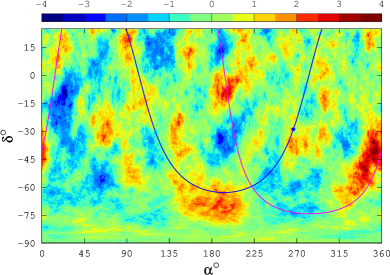
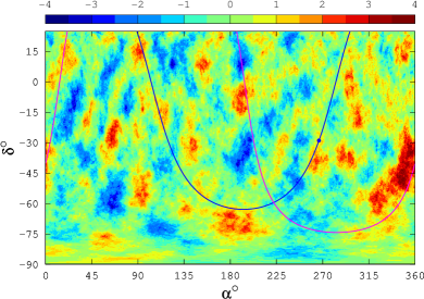
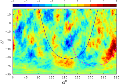
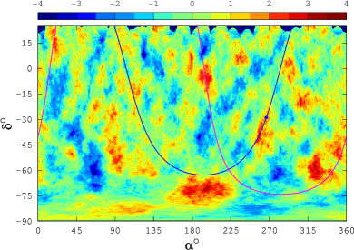
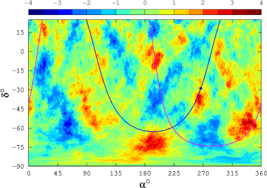
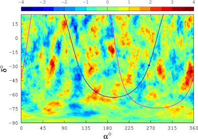
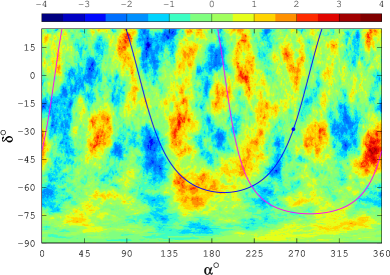
Figure 1: From top to bottom: maps of anisotropy for the main data set, the main data set on the IBG, the LE and HE data sets. The maps are smoothed at $R=8^{\circ}$ (left column) and $R=12^{\circ}$ (right column). Equatorial coordinates are used. The blue curve shows the Galactic plane with the Galactic Center indicated by a bold point. The magenta curves show the Supergalactic plane. Colors indicate the Li–Ma significance of deviation from the expected background.

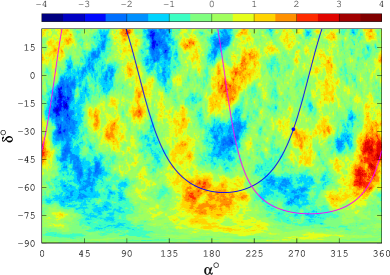
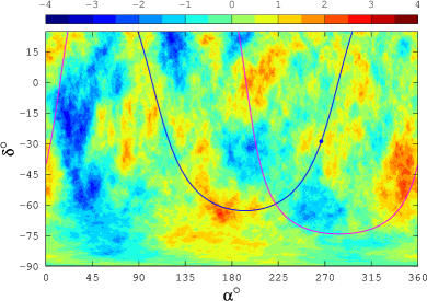
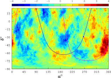
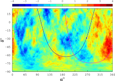
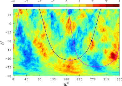
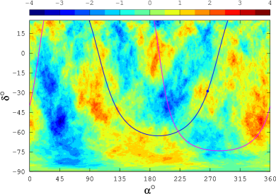
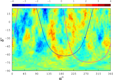
Figure 2: The same as in Fig. 1 but the maps are smoothed at $R=16^{\circ}$ (left column) and $R=20^{\circ}$ (right column).

In the main data set, there are four extended regions of excess (“hot spots”) that deviate from the background by more than 3 standard deviations for $R=8^{\circ}$, with Region D being the most extended and pronounced of them, see the top left panel in Fig. 1 and Table 2. Its two “peaks” are separated from each other by $\approx 14^{\circ}$. Two of the hot spots, namely Region C and Region D, are located near the Supergalactic plane (SGP). An extended Region B can be seen near the GP. Region A is located far from both GP and SGP.

The map of anisotropy obtained for the main data set with the IBG is close to that obtained with the shuffling technique (see the second row in Fig. 1) but Region D becomes more pronounced while the Li–Ma significance decreases for the other hot spots.

There is no counterpart of Region A in the LE data set but Region B becomes more extended and pronounced. To the contrary, both hot spots located near the SGP become less noticeable. Region D splits into two parts with the most pronounced of them being shifted to higher declinations along the SGP. The picture of anisotropy for the HE set is considerably different. Regions A and C become much more pronounced than in the main data set while Region B practically “dissolves.” Region D becomes more compact with its “hottest” part coinciding with one of the peaks in the main data set. The HE set has three other hot spots but $S$ only marginally exceeds three standard deviations for them, see Table 2.

One might expect that hot spots become less pronounced as the angular scale of windows used for the analysis grows but this does not happen to be exactly the case. While the Li–Ma significance for Region A and Region B of the main data set decreases well below three standard deviations for $R=12^{\circ}$, Regions C and D become more pronounced, see the top right panel in Fig. 1 and Table 3. For the main data set on the IBG, only Region D still has $S>3$ and its deviation from the background is also higher than for $R=8^{\circ}$. Notice that Regions B and D are still present in the LE data set but only Region D and Region HE(1) remain in the HE set. One more hot spot appears in the LE set for $R=12^{\circ}$, see Table 3. It is located in the GP with its most pronounced part being $7^{\circ}$–$10^{\circ}$ from the direction to the Galactic Center (on the opposite side of the GP w.r.t. the GC comparing with what was found by AGASA and SUGAR [18, 19] but not confirmed later by Auger [5, 7]). The region can also be seen for $R=8^{\circ}$ both in the LE and in the main data sets but its deviation from the background is less than three standard deviations. Conversely, the flux does not deviate from the background at this location in the HE data set.

Figure 2 shows maps of anisotropy obtained for circular windows of radii $R=16^{\circ}$ and $R=20^{\circ}$. It can be seen that the picture becomes closer to what is expected for isotropy at large scales as $R$ grows. (The Li–Ma significance can be slightly underestimated since the number of events in regions of these radii becomes comparatively large, see a remark above.) There remain no regions in the HE set that deviate from the background by more than $3\sigma$. Only Region D remains in the other data sets for $R=16^{\circ}$ with the Li–Ma significance decreasing. For $R=20^{\circ}$, $S<3$ for Region D in the main data set (on the shuffled background) and only marginally exceeds 3 for the LE set.

A recent study of the large-scale distribution of CRs around 1 EeV performed by the Pierre Auger Collaboration revealed that while it does not contradict isotropy, declination and right ascension of the dipole for the 1–2 EeV energy band are $\alpha\approx 340^{\circ}$, $\delta\approx-35^{\circ}$ with uncertainty $\sim 12^{\circ}$ [16]. The direction correlates with Region D and its counterpart in the HE set. This allows one to suggest that Region D is somehow related to the dipole anisotropy in this energy range.

One can see by comparing Fig. 1 and Fig. 2 how some of the separate regions with an excess or deficit of cosmic rays concatenate as the angular scale of the analysis increases. It is especially clear from Fig. 2 how different are the “patterns” of anisotropy for the LE and HE data sets even though they do not significantly deviate from isotropy.

4 Conclusions

The presented results demonstrate that anisotropy of cosmic rays with energies around 1 EeV might have interesting features at certain intermediate angular scales, including localized regions of excess, and that anisotropy evolves with energy. Still, the study has a serious limitation because of the small amount of data used. On the one hand, calculations performed with other available data reveal that a sample consisting of just one or a few percent of the whole data set only partially reproduces anisotropy of the whole set, and significant differences are possible. On the other hand, such limited data sets as those studied do not allow one to apply more advanced methods of analysis. In particular, it is hardly possible to accurately estimate the dipole anisotropy and to take it into account when studying anisotropy at intermediate scales. In our opinion, it would be interesting if an analysis of anisotropy of cosmic rays around 1 EeV at intermediate angular scales is performed with full data sets of the Auger and Telescope Array experiments. It can provide information concerning the structure of the galactic magnetic field and the fundamental problem of the transition from galactic to extragalactic cosmic rays.

I am glad to thank Bohdan Hnatyk and Peter Tinyakov for stimulating discussions, Miguel Mostafá for help with the data at the preliminary stage of the work, and Daniel Fiorino for the useful communication concerning presentation of the results. GNU Octave was used for the calculations [20].

The study was made with a partial financial support by the Russian Foundation for Basic Research grant 13-02-12175 ofi_m.

References

- [1] J. Linsley, L. Scarsi, P. J. Eccles, et al. Isotropy of cosmic radiation. Phys. Rev. Lett., 8:286–287, 1962.
- [2] O. Deligny and the Pierre Auger Collaboration. Large-Scale Distribution of Arrival Directions of Cosmic Rays Detected at the Pierre Auger Observatory Above 10 PeV. Journal of Physics: Conference Series, 531:012002, 2014. arXiv:1403.6314.
- [3] O. Deligny. Cosmic rays around eV: Implications of contemporary measurements on the origin of the ankle feature. Comptes Rendus Physique, 15:367–375, 2014. arXiv:1403.5569.
- [4] M. Fukushima, D. Ivanov, K. Kawata, et al. TA Anisotropy Summary. In Proceedings of the 33rd International Cosmic Ray Conference, Rio de Janeiro, ID1033. 2013.
- [5] A. Letessier-Selvon for the Pierre Auger Collaboration. Anisotropy Studies Around the Galactic Center at EeV Energies with Auger Data. In Proceedings of the 29th International Cosmic Ray Conference, Pune, volume 7, pages 67–70. 2005.
- [6] B. Revenu for the Pierre Auger Collaboration. Search for localized excess fluxes in Auger sky maps and prescription results. In Proceedings of the 29th International Cosmic Ray Conference, Pune, volume 7, pages 75–78. 2005.
- [7] J. Abraham, M. Aglietta, C. Aguirre, et al. Anisotropy studies around the galactic centre at EeV energies with the Auger Observatory. Astroparticle Physics, 27:244–253, 2007. arXiv:astro-ph/0607382.
- [8] E. M. Santos for the Pierre Auger Collaboration. A search for possible anisotropies of cosmic rays with EeV in the region of the Galactic Centre. In Proceedings of the 30th International Cosmic Ray Conference, Merida, volume 4, pages 171–174. 2008. arXiv:0706.2669.
- [9] B. Revenu for the Pierre Auger Collaboration. Blind searches for localized cosmic ray excesses in the field of view of the Pierre Auger Observatory. In Proceedings of the 33rd International Cosmic Ray Conference, Rio de Janeiro, ID1206. 2013. arXiv:1307.5059.
- [10] H. Lyberis. Study of ultra-high energy cosmic rays with the Pierre Auger Observatory: towards observations of anisotropies in arrival directions? Ph.D. thesis, IPNO, Orsay (France), University of Torino (Italy), 2011.
- [11] K. Kawata, M. Fukushima, D. Ikeda, et al. Search for the Large-Scale Cosmic-Ray Anisotropy at eV with the Telescope Array Surface Detector. In Proceedings of the 33rd International Cosmic Ray Conference, Rio de Janeiro, ID0311. 2013.
- [12] G. Di Sciascio and R. Iuppa. On the Observation of the Cosmic Ray Anisotropy below eV, 2014. arXiv:1407.2144.
- [13] M. Kachelrieß, P. D. Serpico, and M. Teshima. The Galactic magnetic field as spectrograph for ultra-high energy cosmic rays. Astroparticle Physics, 26:378–386, 2007. arXiv:astro-ph/0510444.
- [14] G. L. Cassiday, R. Cooper, B. R. Dawson, et al. Evidence for -eV neutral particles from the direction of Cygnus X-3. Physical Review Letters, 62:383–386, 1989.
- [15] D. E. Alexandreas, D. Berley, S. Biller, et al. A search of the northern sky for ultra-high-energy point sources. The Astrophysical Journal Letters, 383:L53–L56, 1991.
- [16] R. M. de Almeida for the Pierre Auger Collaboration. Constraints on the origin of cosmic rays from large scale anisotropy searches in data of the Pierre Auger Observatory. In Proceedings of the 33rd International Cosmic Ray Conference, Rio de Janeiro, ID0768. 2013. arXiv:1307.5059.
- [17] T.-P. Li and Y.-Q. Ma. Analysis methods for results in gamma-ray astronomy. The Astrophysical Journal, 272:317–324, 1983.
- [18] N. Hayashida, M. Nagano, D. Nishikawa, et al. The anisotropy of cosmic ray arrival directions around 1018 eV. Astroparticle Physics, 10:303–311, 1999. arXiv:astro-ph/9807045.
- [19] J. A. Bellido, R. W. Clay, B. R. Dawson, et al. Southern hemisphere observations of a eV cosmic ray source near the direction of the Galactic Centre. Astroparticle Physics, 15:167–175, 2001. arXiv:astro-ph/0009039.
- [20] J. Eaton, D. Bateman, S. Hauberg, et al. GNU Octave version 3.8.1 manual: a high-level interactive language for numerical computations. CreateSpace Independent Publishing Platform, 2014. ISBN 1441413006.