On the chaotic behavior of the Primal–Dual Affine–Scaling Algorithm for Linear Optimization

Abstract

We study a one-parameter family of quadratic maps, which serves as a template for interior point methods. It is known that such methods can exhibit chaotic behavior, but this has been verified only for particular linear optimization problems. Our results indicate that this chaotic behavior is generic.

We study a one-parameter family of quadratic maps on a projective simplex, which has been derived from an interior point method, known as the primal-dual Affine Scaling method JansenRoosTerlaky . This particular method neatly handles both the primal and the dual variables in one step, enabling us to derive a one-parameter family, independently of the underlying linear optimization problem. We study the bifurcations of this one-parameter family and find that they are almost identical to those that have previously been found by Castillo and Barnes Barnes for a specific linear optimization problem, using another interior point method. This indicates, experimentally and non-rigorously, that the route to chaos in our one-parameter family is typical for general interior point methods.

I Introduction

In linear optimization one wants to compute the maximum value of a linear objective function under linear inequality constraints. There exist many algorithms that solve LO problems by iteration. The classical algorithm is the simplex method, which produces an exact solution. It runs through the extremal points of the convex set that satisfies the constraints (the feasible set), improving the value of objective function in each step, halting at an extremal point that produces the maximum value. The simplex method runs from one boundary point of the feasible set to the next. Interior point methods run through the interior of the feasible set. Historically, the first such method is the affine scaling algorithm (AFS) method of Dikin, which remained unnoticed until 1985. The work of Karmarkar int:Karmarkar2 sparked a large amount of research in polynomial–time methods for LO, and gave rise to many new and efficient interior point methods (IPMs) for LO. For a survey of this development we refer to the books of Wright int:SWright9 , Ye BookYe , Vanderbei Vanderbei and Roos et al. RoosTerlakyVial2 . An IPM starts from an arbitrary initial point $x_{0}$ in the interior and constructs a sequence $x_{n}$ that converges to a maximum $x^{*}$. An IPM is a dynamical system which solves the LO problem, provided that the $\omega$-limit of $x_{0}$ consists of maxima of the objective function $f$. If there is only one such maximum, then the LO problem is called non-degenerate. In this case, the IPM solves the LO problem provided that it converges to the maximum.

Any LO problem can be converted to a dual problem in which one needs to find the minimum value of a dual linear objective function under dual constraints. If $f$ is the objective function of the primal problem and if $g$ is the objective function of the dual problem, then $f(x)\leq g(y)$ for all feasible $x$ and all $y$. To solve an LO problem it therefore suffices to close the duality gap and find $x^{*},y^{*}$ such that $f(x^{*})=g(y^{*})$. According to the minimax theorem, such $x^{*},y^{*}$ exist and apart from a primal sequence $x_{n}$ most IPM’s also produces a dual sequence $y_{n}$, halting as soon as the duality gap $g(y_{n})-f(x_{n})$ reaches a value which is below the desired accuracy threshold. A primal problem that is non-degenerate may have a degenerate dual problem, in which case the orbit $y_{n}$ may have a non-trivial $\omega$-limit set. We will study such an LO problem at the end of this paper and find that the dual dynamical system contains a hyperbolic attractor.

The simplex method runs from one extremal point to the next, but an IPM uses a variable step size $\alpha$. For each feasible $x$ the algorithm produces a vector $v$ such that $x+\alpha v$ is contained in the feasible set for $0\leq\alpha\leq 1$ and such that $x+v$ is in the boundary of the feasible set. The step size $\alpha$ is fixed during iteration and is chosen $<1$ so that the orbit $x_{n}$ is contained in the interior of the feasible set. An IPM therefore is a one-parameter family of dynamical systems. It is well known that an IPM may not converge if $\alpha$ is too large. One of the best studied algorithms is the Affine Scaling method (AFS) which was proposed by Dikin and which has been further developed by Vanderbei et al. Vanderbeietal It is known TsuchiyaMuramatsu that AFS converges if $\alpha\leq 2/3$ and that it need not converge if $\alpha>2/3$, see twothirds . It is also known that AFS behaves chaotically in the dual variables for $\alpha>2/3$, as has been found by Castillo and Barnes Barnes and Mascarenhas Mascarenhas .

I.1 Outline of our paper

The previous studies of chaotic behavior in interior point methods were carried out for specific problems: one considers an LO problem, applies the algorithm and analyzes the resulting dynamical system. In this paper, we take a different approach. We consider the primal-dual AFS that was proposed by Jansen et al. JansenRoosTerlaky . It has the nice property that it be presented in a such a form that its low order terms do not depend on the original LO problem. By ignoring the higher order terms, we obtain a one-parameter family of dynamical systems, which we call the Dikin process, that is the same for all LO problems. Of course, the Dikin process is not an IPM anymore. However, the bifurcations that we establish for the Dikin process are the same as the bifurcations that have previously been found by Castillo and Barnes for their specific LO problem. This indicates, experimentally and non-rigorously, that the chaotic behaviour of the Dikin process represents that of general interior point methods.

Our paper is organized as follows. We first recall the primal-dual AFS method for solving LO problems. We then derive the one-parameter family of dynamical systems, and analyze it for increasing values of a parameter $\theta$. We show that the system behaves chaotically as $\theta$ increases beyond $2/3$. We supplement this analysis experimentally by Feigenbaum diagrams. In the final section, we compare our results to an IPM that arises from a specific LO problem.

I.2 Notation

We reserve the symbol $e\in\mathbb{R}^{n}$ for the vector of all ones. For a vector $x$, the capital $X$ denotes the diagonal matrix with the entries of $x$ on the diagonal. Furthermore, if $f:\mathbb{R}\rightarrow\mathbb{R}$ is a function and $x\in\mathbb{R}^{n}$, then we denote by $f(x)$ the vector $(f(x_{1}),\dots,f(x_{n}))$. If $s$ is another vector, then $xs$ will denote the coordinatewise product of $x$ and $s$ and $x/s$ will denote the coordinatewise quotient of $x$ and $s$. In other words, $xs=Xs$ and $x/s=S^{-1}x$. Finally, $\|.\|$ denotes the $l_{2}-$norm.

II A recap of the Primal-dual affine scaling method

In linear optimization, the notion of affine scaling has been introduced by Dikin int:Dikin1 as a tool for solving the (primal) problem in standard format

$$(P)\;\;\;\qquad\min\{c^{T}x\,:\,Ax=bx\geq 0\}.$$

The underlying idea is to replace the nonnegativity constraints $x\geq 0$ by the ellipsoidal constraint

$$\|\bar{X}^{-1}({\bar{x}}-x)\|\leq 1,$$ (1)

where $\bar{x}$ denotes some given interior feasible point, and $\bar{X}$ the diagonal matrix corresponding to $\bar{x}$. The resulting subproblem is easily solved and renders a new interior feasible point with a better objective value. Dikin showed, under the assumption of primal nondegeneracy, that this process converges to an optimal solution of $(P)$.

Every known method for solving $(P)$ essentially also solves the dual problem

$$(D)\;\;\;\qquad\max\{b^{T}y\,:\,A^{T}y+s=cs\geq 0\}$$

by closing the duality gap between $c^{T}x$ and $b^{T}y$, which equals $x^{T}s$. Our basic assumption is that a primal-dual pair $(x,s)$ of feasible solutions exists and that $A$ is an $m\times n$ matrix of rank $m$ for $m<n$. A pair of feasible vectors $x^{*},s^{*}$ solves $(P)$ and $(D)$ if and only if they are orthogonal. Since $x^{*}\geq 0$ and $s^{*}\geq 0$, this means that the coordinatewise product $x^{*}s^{*}$ is equal to the all-zero vector. The primal-dual AFS method that we consider in this paper has been proposed by Jansen et al. JansenRoosTerlaky . In primal-dual AFS, Dikin’s ellipsoidal constraint (1) is replaced by a constraint that includes both the primal and the dual variable:

$$\|\bar{X}^{-1}({\bar{x}}-x)+\bar{S}^{-1}({\bar{s}}-s)\|\leq 1,$$ (2)

where $\bar{S}$ denotes the diagonal matrix corresponding to the slack vector $\bar{s}$. In this notation, $(\bar{x},\bar{s})$ is the original pair of primal vector and slack vector and $(x,s)$ is an updated pair. The differences $\Delta x=x-\bar{x}$ and $\Delta s=s-\bar{s}$ are called the primal-dual AFS directions.

For non-negative $x,s$ let $v=(xs)^{1/2}$ be the coordinatewise square root of the coordinatewise product and let $v^{k}$ be the coordinatewise power of $v$. Jansen et al. have shown that the directions $\Delta x$ and $\Delta s$ can be derived from the vector

$$p_{v}=-\frac{v^{3}}{\|v\|^{2}}$$

by first projecting $p_{v}$ onto the null space (for $\Delta x$) and the row space (for $\Delta s$) of $AD$, with $D=XS^{-1}$, and then rescaling the result by a coordinatewise product. More specifically, if $d=(x/s)^{1/2}$ then

$$\Delta x=dP_{AD}(p_{v}),\ \Delta s=d^{-1}Q_{AD}(p_{v})$$

where $P_{AD}$ and $Q_{AD}$ denote the orthogonal projections onto the null space of $AD$ and the row space of $AD$, respectively. These projections recombine in the Dikin ellipsoid to

$$X^{-1}\Delta x+S^{-1}\Delta s=-\frac{v^{2}}{\|v^{2}\|}.$$ (3)

This gives the primal-dual AFS directions but not the size of the step, which is controlled by an additional parameter $\alpha$. It is known that the iterative process $x\mapsto x+\alpha\Delta x,s\mapsto s+\alpha\Delta s$ converges to a solution if $\alpha<1/\left(15\sqrt{n}\right)$.JansenRoosTerlaky This is of course a significant restriction on the step size, and primal-dual AFS is not often used in practice.

III Derivation of the Dikin process

Starting with a primal-dual feasible pair $(x,s)$, the next iterated pair is given by

$$x^{+}=x+\alpha\Delta x=s+\alpha\Delta s,$$

and hence we have

$$x^{+}=xs+\alpha\left({x\Delta s+s\Delta x}\right)+\alpha^{2}\Delta x\Delta s.$$

The vectors $\Delta x$ and $\Delta s$ are orthogonal. If the AFS iterations are close to a solution, then $\Delta x$ and $\Delta s$ will be relatively small, and the product $\Delta x\Delta s$ will be negligible. If we ignore the quadratic term, i.e., if we assume that the coordinatewise product $\Delta x\Delta s$ is equal to zero, then the reduction of $xs$ is proportional to $x\Delta s+s\Delta x$, which can be rewritten to

$$xs\left(x^{-1}\Delta x+s^{-1}\Delta s\right).$$

Observe that $x^{-1}\Delta x+s^{-1}\Delta s$ is equal to the left-hand side in $(\ref{sum})$. So if we ignore the quadratic term, and if we use equation $(\ref{sum})$, then we find that

$$x^{+}=xs+\alpha\left({x\Delta s+s\Delta x}\right)=xs-\alpha\frac{x^{2}s^{2}}{\|xs\|}=xs{e-\alpha\frac{xs}{\|xs\|}}.$$

Recall that $e$ denotes the all-one vector, so we may also write this as

$$x^{+}=xs{e-\alpha\frac{xs}{\|xs\|}}.$$

Now we have arrived at an iterative process for the product vector $xs$. Since we require $x\geq 0$ and $s\geq 0$, we need to require $xs\geq 0$ in the iterative process, and the maximal step size is equal to

$$\alpha_{\max}=\frac{\|xs\|}{\max{xs}}$$

Defining

$$\theta=\frac{\alpha}{\alpha_{\max}}=\alpha\frac{\max{xs}}{\|xs\|}$$

and writing $w=xs$ we get

$$w^{+}=w{e-\theta\frac{w}{\max{w}}}\quad\theta\in[0,1].$$

This iterative process depends on a parameter $\theta$ which is related to the original step size by $\alpha=\theta\alpha_{max}$. If $w$ has coordinates that are approximately equal (in optimization one says that $w$ is ‘close to the central line’), then $\alpha_{max}\approx\sqrt{n}$. In general, $1\leq\alpha_{max}\leq\sqrt{n}$.

We make one further reduction. If $u=\lambda w$ for a scalar $\lambda$ then $u^{+}=\lambda w^{+}$, so the iterative process preserves projective equivalence. We may therefore reduce our system up to projective equivalence by scaling vectors so that their maximum coordinate is equal to one. If we consider vectors up to projective equivalence, then we obtain our Dikin process:

$${\bar{w}}^{k}=w^{k}{e-\theta w^{k}}\quad w^{k+1}=\frac{{\bar{w}}^{k}}{\max{\bar{w}}^{k}}\quad k=0,1,\ldots$$ (4)

The Dikin process involves two steps: multiplication and scaling. To describe the process more succinctly we use the map $f_{\theta}(x)=x(1-\theta x)$. The Dikin process is then given by:

$$w^{k+1}=f_{\theta}(w^{k})/\max\{f_{\theta}(w^{k})\}.$$ (5)

Note that $f_{\theta}$ is a higher-dimensional analog of the logistic map on the unit interval. For each coordinate we apply the same quadratic map, and the only interaction between the coordinates is induced by the scaling. The Dikin process does not solve the original LO problem. Its significance derives from the fact that it does not depend on the LO problem and that its bifurcations can be analyzed in a standard way.

IV Bifurcation analysis

We analyze the Dikin process $f_{\theta}$, for increasing values of $\theta$. We suppress the subscript $\theta$ in $f_{\theta}$ and simply write the Dikin process as

$$w^{k+1}=f(w^{k})/\max\{f(w^{k})\}.$$ (6)

Note that $f$ has a global maximum $f(1/2\theta)=1/4\theta$ and that we scale $f$ such that all coordinates take values $\leq 1$.

IV.1 $\theta\leq 2/3$: the process converges to $e$

If $\theta\leq 1/2$ then the global maximum of $f$ is $\geq 1$, which is outside the domain of our coordinates. The value of each coordinate increases during iteration. By monotonicity the limit of $w^{k}$ exists and it is a fixed point under iteration. The only fixed point is $e$ and therefore $w^{k}$ converges to the all-one vector $e$ if $\theta\leq 1/2$.

We now argue that $e$ remains the global attractor if $\theta\leq 2/3$. If $\theta>1/2$ then $f$ is unimodal and point symmetric with respect to its maximum $1/2\theta$:

$$f\left(\frac{1}{2\theta}+z\right)=f\left(\frac{1}{2\theta}-z\right).$$ (7)

Under iteration of $f$ all orbits eventually end up in the interval $[1-1/\theta,1]$. In particular, for every initial $w^{0}$ it eventually holds that $\min{w^{k}}\geq 1/\theta-1$. We need to show that $\min w^{k}$ in fact converges to $1$ if $1/2\leq\theta\leq 2/3$. By the point symmetry in (7), if we replace the coordinates $w_{i}<1/2\theta$ in $w^{k}$ by their reflections $1/\theta-w_{i}$, then this does not affect $w^{k+1}$. We may therefore assume that $\min w^{k}\geq 1/2\theta$. Let $x=\min w^{k}\geq 1/2\theta$. Since $f$ is decreasing for $x\geq 1/2\theta$ we have that $f(x)=\max f(w^{k})$ and $f(1)=\min f(w^{k})$. Therefore the minimum coordinate of $w^{k+1}$ is given by

$$h(x)=\frac{f(1)}{f(x)}=\frac{1-\theta}{x(1-\theta x)}.$$ (8)

To prove that the process converges to $e$, it now suffices to prove that $h(x)\geq x$, because this implies that the limit of $h^{k}(x)$ exists and is equal to the unique fixed point of $h$. Now $h(x)\geq x$ can be rewritten as

$$\theta x^{3}-x^{2}+1-\theta\geq 0.$$ (9)

The derivative $(3\theta x-2)x$ of the cubic $\theta x^{3}-x^{2}+1-\theta$ is negative on the unit interval, by our assumption that $\theta\leq 2/3$. So the cubic has its maximum at $0$ and its minimum at $x=1$, which is a zero of the cubic. Hence the inequality $h(x)\geq x$ holds and we conclude that $w^{k}$ also converges to $e$ if $1/2\leq\theta\leq 2/3$.

IV.2 $2/3<\theta\leq\frac{1+\sqrt{5}}{4}$: convergence to a point of period two.

We will see that if $2/3<\theta\leq\frac{1+\sqrt{5}}{4}$, then the minimum coordinate and the maximum coordinate interchange under iteration, while all other coordinates either converge to the minimum of the maximum. We can thus ignore these other coordinates, and observe that the Dikin process on the minim and maximum coordinate is given by $(x,1)\to(1,h(x))\to(h^{2}(x),1)\to\cdots$, with $h$ as in (8). Observe that a fixed point of $h$ produces a point of period two for this process.

If $\theta>2/3$ then $h$ has a unique fixed point $r\in(0,1)$, which can be found by solving the cubic equation $h(x)=x$ that we already encountered in equation (9). This cubic is divisible by $x-1$, so we find that $r$ satisfies the quadratic equation

$$\theta r^{2}+(\theta-1)r+(\theta-1)=0.$$ (10)

The positive solution for $r$ is equal to

$$r=\frac{1-\theta+\sqrt{(1-\theta)^{2}+4\theta(1-\theta)}}{2\theta},$$ (11)

which is $\leq 1$ if and only if $\theta\geq 2/3$. The cubic equation $h(x)=x$ has zeros in $1,r$ and the third zero $s$ is negative. In particular, $h(x)>x$ on $(s,r)$ and $h(x)<x$ on $(r,1)$ and we find that $r$ is the global attractor of $h$ in the interval $[1/\theta-1,1)$. Note that $r$ is not a global attractor in the closed interval $[1/\theta-1,1]$ since $h(1)=1$ is a fixed point.

Since $r$ is an attractor, the two-dimensional process $(x,1)\to(1,h(x))$ converges to an orbit of period two if $\theta>2/3$. We note that this particular limit behavior has also been observed by Hall and Vanderbei twothirds for the (primal) AFS method.

Since all coordinates eventually increase above $1-1/\theta$ we may as well assume that $\min w^{0}\geq 1/\theta-1$. The minimum coordinate of $f(w^{0})$ then has value $f(1)=1-\theta$ and the maximum coordinate has value $\leq 1/4\theta$. Therefore, $\min w^{1}\geq 4\theta(1-\theta)$. If in fact $\min w^{1}\geq 1/2\theta$, then we can restrict out attention to the mimimum and the maximum coordinate. This would be the case if $4\theta(1-\theta)\geq 1/2\theta$, which leads us to the cubic equation

$$8\theta^{2}(1-\theta)-1=0\Longleftrightarrow(2\theta-1)(1-2\theta-4\theta^{2})=0.$$

The two roots of the quadratic are $\frac{1\pm\sqrt{5}}{4}$, and so we conclude that we may indeed restrict our attention to the minimum and the maximum coordinate if $\frac{1}{2}<\theta\leq\frac{1+\sqrt{5}}{4}$.

Suppose $\theta\leq\frac{1+\sqrt{5}}{4}\approx 0.809$ and consider an initial condition $w^{0}=(w_{1},\dots,w_{n})$ with increasing coordinates $w_{1}\leq w_{2}\leq\dots\leq w_{n}=1$ and such that $w_{1}\geq 1/2\theta$. For an intermediate coordinate $w_{i}$ the process is given by $w_{i}\to\frac{w_{i}(1-\theta w_{i})}{w_{1}(1-\theta w_{1})}.$ Now the minimum coordinate converges to $r$ so we may as well put $w_{1}=r$, in which case we get that $w_{i}\to g(w_{i})$ for the map

$$g(x)=\frac{x(1-\theta x)}{r(1-\theta r)}.$$

This map $g$ keeps track of the Dikin process $w^{k}$ on a fixed coordinate. We now prove that the $\omega$-limit of $g$ is Lebesgue a.e. equal to $\{r,1\}$, which will show that a.e. point converges to a point of period two. This comes down to a straightforward computation, which is carried out in the paragraph below.

First note that $g(r)=1$ and that $g(1)=h(r)=r$ so that $g$ has a fixed point $s\in(r,1)$ as is illustrated by the graph of $g^{2}$ in the figure below. We leave it to the reader to verify that $g$ has a unique fixed point in $(r,1)$ at $s=(r+\theta-1)/r\theta$.

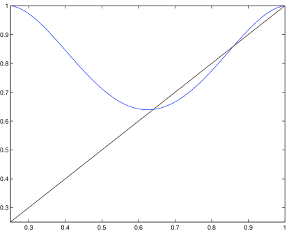
Figure 1: The function $g^{2}$ on the interval [1/4,1] for $\theta=0.8$ plotted against the diagonal.

The derivative of $g$ is given by

$$g^{\prime}(x)=\frac{1-2\theta x}{r(1-\theta r)}=\frac{r(1-2\theta x)}{1-\theta},$$ (12)

where we use that $1-\theta=r^{2}-\theta r^{3}$. Note that $g(x)=x$ is a quadratic equation with solutions $x=0$ and $x=s$. The equation $g^{2}(x)=x$ is an equation of degree four with solutions $0,r,s,1$. It follows that $g^{2}(x)\not=x$ on the two subintervals $(r,s)\cup(s,1)$ and that $g^{2}(x)>x$ on the one interval while $g^{2}(x)<x$ on the other interval. Using equation (12), and using that $rs\theta=r+\theta-1$, we find that the derivative at $s$ is

$$g^{\prime}(s) = \frac{r\left(1-2\theta s\right)}{1-\theta}=\frac{2-r-2\theta}{1-\theta}.$$

To prove that $s$ is unstable, we need to verify that $\frac{2-r-2\theta}{1-\theta}<-1$, or equivalently, that $r>3-3\theta$. Substituting (11) for $r$ and simplifying equations we end up with $(1-\theta)+\sqrt{(1-\theta)^{2}+4\theta(1-\theta)}>6\theta(1-\theta).$ Taking squares to remove the root gives $(1-\theta)^{2}+4\theta(1-\theta)>(6\theta-1)^{2}(1-\theta)^{2}.$ which simplifies to $1+3\theta>(6\theta-1)^{2}(1-\theta)$. Collecting all terms and dividing by $\theta$ we finally arrive at the inequality $9\theta^{2}-12\theta+4>0$, or equivalently, $(3\theta-2)^{2}>0$. This obviously holds if $\theta>2/3$. It follows that $g^{2}(x)<x$ on $(r,s)$ and that $g^{2}(x)>x$ on $(s,1)$. This completes our computation and we conclude that if $2/3<\theta\leq\frac{1+\sqrt{5}}{4}$, then the $\omega$-limit is Lebesgue a.e. equal to an orbit of period two. The coordinates of these periodic points are either equal to $r$ or $1$.

IV.3 Persistence of period two.

For generic period doubling bifurcations in smooth dynamical systems, the parameter curve of the periodic points of period $2n$ is parabolic and intersects the curve of the periodic point of period $n$ transversally. At the point of intersection, the period $n$ point changes from stable to unstable, or vice versa. Curiously, this scenario fails in at least the first two periodic doublings in our Feigenbaum diagrams, in particular see Figure 3. Our numerical experiments show that the period two limit cycle persists beyond $\frac{1+\sqrt{5}}{4}$. It is indeed possible to prove that the period two point persist, but the analysis gets involved. We limit ourselves to the case that $w$ has three coordinates. Assuming that the coordinates are ordered $x<y<1$ we can write

$$(x,y,1) \mapsto \left(1,\frac{y(1-\theta y)}{x(1-\theta x)},\frac{1-\theta}{x(1-\theta x)}\right)$$

$$\mapsto \left(\frac{x(1-\theta x)}{1-\theta\frac{1-\theta}{x(1-\theta x)}}\ ,\ \frac{y(1-\theta y)}{1-\theta}\frac{1-\theta\frac{y(1-\theta y)}{x(1-\theta x)}}{1-\theta\frac{1-\theta}{x(1-\theta x)}}\ ,\ 1\right)$$

so we can describe the second iterate by the function

$$F(x,y)=\left(\frac{x(1-\theta x)}{1-\theta\frac{1-\theta}{x(1-\theta x)}}\ ,\ \frac{y(1-\theta y)}{1-\theta}\frac{1-\theta\frac{y(1-\theta y)}{x(1-\theta x)}}{1-\theta\frac{1-\theta}{x(1-\theta x)}}\right).$$

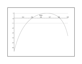
Figure 2: Value of the second ‘transversal’ eigenvalue $\frac{\partial F_{2}}{\partial y}(r,r)$ as function of $\theta$.

This function preserves the diagonal, on which we have the two-dimensional process, which as we have seen already has a period two global attractor for $\theta>2/3$. So, the instability has to occur in the direction transversal to the diagonal. We can study this stability by taking the derivative

$$DF(x,y)=\left[\begin{array}[]{ll}\frac{\partial F_{1}(x,y)}{\partial x}&\frac{\partial F_{2}(x,y)}{\partial x}\\ 0&\frac{\partial F_{2}(x,y)}{\partial y}\end{array}\right]$$

where the partial derivatives on the diagonal of the matrix $\frac{\partial F^{1}(x,y)}{\partial x},\frac{\partial F_{2}(x,y)}{\partial y}$ are equal to

$$\frac{(x-3\theta x^{2}-2\theta+2\theta^{2}+2\theta^{2}x^{3}+4\theta^{2}x-4\theta^{3}x)x(1-\theta x)}{(-x+\theta x^{2}+\theta-\theta^{2})^{2}}$$

and

$$\frac{x-\theta x^{2}-2y\theta+6y^{2}\theta^{2}-2x^{2}\theta+2y\theta^{2}x^{2}-4y^{3}\theta^{3}}{(-x+\theta x^{2}+\theta-\theta^{2})\cdot(-1+\theta)}.$$

Maple computations show that fixed point becomes unstable at $\theta=0.8499377796$, when the eigenvalue $\frac{\partial F_{2}(r,r)}{\partial y}$ becomes equal to $-1$. At this value of $\theta$ we expect $(r,r,1)$ to become unstable, splitting off a stable period $4$ point in a period doubling bifurcation, which is confirmed by the Feigenbaum diagrams below. In our computational results for real LO problems, we find that the limit two cycle persists slightly beyond the threshold of $\theta=0.8499377796$.

IV.4 $\theta>\frac{1+\sqrt{5}}{4}$: comparison to the logistic family.

It is hard to extend the bifurcation analysis for $\theta\geq\frac{1+\sqrt{5}}{4}$, since the degree of the algebraic equations increases and periodic points cannot be found in closed form. However, using the similarity between the Dikin process and the logistic mapFeigenbaum $Q_{\theta}:x\mapsto 4\theta x(1-x)$, we can prove that stable periodic points of higher order appear if $\theta$ increases beyond $\frac{1+\sqrt{5}}{4}$. In particular, we shall now show that if the critical point $c=\frac{1}{2}$ is $m$-periodic under $Q_{\theta}$ then the Dikin process has a locally stable $m$-periodic orbit, provided the number of coordinates $n\geq m$.

Assume that the first $m$ coordinates $w_{i}^{k}$ of the vector $w^{k}$ are equal to $Q_{\theta}^{i}(c)/\theta$ (so the coordinates are not put in increasing order here). In particular, $w_{m}^{k}=c/\theta=1/2\theta$, and $f_{\theta}(w_{m}^{k})=1/4\theta=\max\{f_{\theta}(x)\}$. Then $w_{i}^{k+1}=4\theta f_{\theta}(w_{i}^{k})=4\theta w_{i}^{k}(1-\theta w_{i}^{k})$. The linear scaling $h(x)=\theta x$ conjugates this to $Q_{\theta}$, since $h^{-1}\circ Q_{\theta}\circ h(x)=4\theta x(1-\theta x)$. Since the the critical point of $Q_{\theta}$ is periodic by our assumption, the critical point of $f_{\theta}$ is periodic too: $w_{i}^{k+1}=w_{(i\bmod m)+1}^{k}$ for $i=1,\dots,m$, and $w^{k+1}_{m-1}=1/2\theta$. In particular, the scaling remains the same for all iterates.

This periodic orbit attracts the coordinates $w_{i}$ for $m<i\leq n$ and Lebesgue-a.e. initial choice of $w_{i}$. Let us now verify that the orbit is also stable under small changes in the coordinates $w_{i}$ for $1\leq i\leq m$. Renaming these $w_{i}$ to $y_{i}$, $i=1,\dots,m$, where $y_{m-1}=1/2\theta$, $y_{m}=1$, $y_{1}=f(1)/f(y_{m-1})$ and $y_{i+1}=f(y_{i})/f(y_{m-1})$ for $1\leq i<m$, we can describe them by the map

$$F(y_{1},\dots,y_{m-1},1)=\left(\frac{f(1)}{f(y_{m-1})},\dots,\frac{f(y_{m-2})}{f(y_{m-1})},1\right)$$ (13)

The final coordinate is redundant, so $DF$ is an $(m-1)\times(m-1)$ matrix. Recall that $f^{\prime}(x)=1-2\theta x$. Therefore $DF(y)$ is equal to

$$\left(\begin{array}[]{ccccr}0&\dots&0&\ -(1-2\theta y_{m-1})\frac{f(1)}{f(y_{m-1})^{2}}\\[2.84526pt] \frac{1-2\theta y_{1}}{f(y_{m-1})}&\dots&0&\ -(1-2\theta y_{m-1})\frac{f(y_{1})}{f(y_{m-1})^{2}}\\[2.84526pt] 0&\dots&0&\ -(1-2\theta y_{m-1})\frac{f(y_{2})}{f(y_{m-1})^{2}}\\[2.84526pt] \vdots&&\vdots&\vdots&\\[2.84526pt] 0&\dots&\frac{1-2\theta y_{m-2}}{f(y_{m-1})}&\ -(1-2\theta y_{m-1})\frac{f(y_{m-2})}{f(y_{m-1})^{2}}\end{array}\right)$$

and since $y_{m-1}=1/2\theta$, the right-most column is zero. Therefore all eigenvalues are zero, and $DF^{n}$ is a contraction. We conclude that the structure of the Feigenbaum map of the logistic family must be present within the Feigenbaum diagrams of the Dikin process. However, we made no estimate on the basin of attraction of the periodic points, and our numerical results indicate that these basins are small.

IV.5 The process converges to a periodic point for $\theta$ near $1$.

Surprisingly, it is possible to determine the limit of $w^{k}$ for $\theta$ arbitrarily close to $1$. To conclude our bifurcation analysis, we show that for $\theta$ close to $1$ the Dikin process has a locally stable point of period $n$, i.e., the period is equal to the dimension.

Let $y$ be any point with maximal coordinate $1$ and all other coordinates $\leq\frac{1}{2\theta}$. As before, we assume $\min y\geq 1/\theta-1$ and this implies that $f(1)$ is the minimal coordinate of $w^{1}$. We arrange the coordinates of $y$ in non-decreasing order. Then $f(y_{m-1})$ is the largest coordinate among all the $f(y_{k})$, so we scale by this number and we arrange the coordinates of $w^{1}$ in non-decreasing order. The dynamic process can then be described by the map $F(y_{1},\dots,y_{m-1},1)=\left(\frac{f(1)}{f(y_{m-1})},\dots,\frac{f(y_{m-2})}{f(y_{m-1})},1\right)$ of equation $(\ref{Fmap})$, and therefore we find cyclic periodicity if $f(y_{k})/f(y_{m-1})=y_{k+1}$ and $f(1)/f(y_{m-1})=y_{1}$. Fix $y_{m-1}<1/2\theta$ and define a map $g(x)=f(x)/f(y_{m-1})$. Note that $y$ has the required cyclic periodicity if

$$y_{m-1}=g(y_{m-2})=\cdots=g^{m-2}(y_{1})=g^{m-1}(1).$$

By the point symmetry of $f$ in (7), we may replace $g^{m-1}(1)$ by $g^{m-1}(1/\theta-1)$. If we take $y_{m-1}=1/2\theta$ then a sufficient condition for the cyclic periodic point to exist is

$$g^{m-1}(1/\theta-1)\leq 1/2\theta.$$ (14)

This inequality is satisfied if $\theta$ is sufficiently close to $1$. Now $g$ increases as $y_{m-1}$ decreases, so once the condition is satisfied, there exists an $y_{m-1}$ such that $g^{m-1}(1/\theta-1)=y_{m-1}$. To compute the stability of this orbit, we cannot use anymore that the right-most column of $DF$ vanishes, because now $y_{m-1}<1/2\theta$. Fortunately, $DF$ is of a simple form

$$DF(y)=\left(\begin{array}[]{ccccc}0&0&\dots&0&-c_{1}\\[2.84526pt] \ d_{1}&0&&\vdots&-c_{2}\\[2.84526pt] 0&\ d_{2}&\quad\ddots&&-c_{3}\\[2.84526pt] \vdots&&\ddots&&\vdots\\[2.84526pt] 0&\cdots&&d_{m-1}&-c_{m}\end{array}\right)$$

where $d_{1}>d_{2}>\ldots>d_{m-1}>0$ and $0<c_{1}<c_{2}<\ldots<c_{m}<1$. This follows from the fact that $y_{1}<y_{2}<\cdots<y_{m-1}\leq 1/2\theta$ and that $f$ is increasing on $[y_{1},y_{m-1}]\subset[0,\frac{1}{2\theta}]$. In order to estimate the eigenvalues of $DF$ we use the classical result of Eneström-KakeyaEnestrom that a polynomial $p(z)=\sum_{k=0}^{m}a_{k}z^{k}$ with all coefficients $a_{i}\geq 0$ has zeros in the annulus $\alpha\leq|z|\leq\beta$, where

$$\alpha=\min\left\{\frac{a_{k}}{a_{k+1}}\right\},\ \beta=\max\left\{\frac{a_{k}}{a_{k+1}}\right\}.$$

Claim: If $c_{i}d_{i}<c_{i+1}$ for all $i\leq m-1$, then all eigenvalues of $DF$ are in the open unit disc.

Abbreviate $A=DF$ and let $p(\lambda)=\det(\lambda I_{m}-A)=\sum_{k=0}^{m}a_{k}\lambda^{k}$ be the characteristic polynomial of $A$. We will show by induction that the coefficients are decreasing. More precisely $1=a_{m}>\cdots>a_{0}>0$ and $a_{0}=c_{1}d_{1}\cdots d_{m-1}$. The proof of the claim is by induction. The claim is obvious for $m=1$. Assume that the claim is true for $m-1$. The characteristic polynomial is equal to

$$\lambda\det(\lambda I_{m-1}-A_{11})+(-1)^{m-1}c_{1}\cdot(-d_{1})\cdots(-d_{m-1}),$$

where $A_{11}$ is the $(1,1)$-minor matrix of $A$. By the inductive hypothesis, $\det(\lambda I_{m-1}-A)$ has decreasing coefficients and constant coefficient $c_{2}\cdot d_{2}\cdots d_{m-1}$. If we rewrite $a_{0}=\frac{c_{1}}{c_{2}}\cdot d_{1}\cdot a_{1}<a_{1}$, then the claim follows. We now compute

$$\frac{c_{i}}{c_{i+1}}\cdot d_{i}=\frac{f(y_{i-1})}{f(y_{i})}\frac{1-2\theta y_{i}}{f(y_{m-1})}=\frac{1-2\theta y_{i}}{1-\theta y_{i}}<1.$$

which demonstrates that $c_{i}d_{i}<c_{i+1}$, as claimed. By the Eneström-Kakeya Theorem, the roots of $p(\lambda)$ are all in the open unit disc. Hence $DF^{m}$ is a contraction at $(y_{1},\dots,y_{m})$ for $\theta$ sufficiently close to $1$.

Our numerical simulations suggest that the set of initial values $w^{0}$ that converge to this periodic point is large and has (nearly) full measure, as illustrated by the Feigenbaum diagrams in the next section.

V Feigenbaum diagrams

The Dikin process is defined in aribtrary dimensions, so in our Feigenbaum diagrams we have to project $n$-dimensional $\omega$-limits onto one dimension. We have chosen to simply plot one single coordinate of the $\omega$-limit set.

Figure 3: Feigenbaum diagram for the process on three coordinates. Above: $\omega$-limit of a random coordinate, and below: $\omega$-limit of the middle coordinate. Note that the bifurcation at 0.8499377796 produces a period four point.

The Feigenbaum diagrams seem to exhibit the usual structure of period doubling cascades of the logistic family $Q_{\theta}:x\mapsto 4\theta x(1-x)$, $\theta\in[0,1]$. It is well-known that for $Q_{\theta}$, between two period doubling bifurcations, there is a parameter where the critical point $c=\frac{1}{2}$ is periodic. We proved above that this periodic point should then also appear as a stable periodic point in the Dikin process, provided the dimension exceeds the period. Since our examples have small dimension, we do not see much of the period doubling cascade of the logistic family.

To illustrate the consequence of the choice of the projection, compare the Feigenbaum diagrams in Figure 3. In the top figure we plot the $\omega$-limit set of a random coordinate. Below we choose the middle coordinate of the ordered vector. We see that the process bifurcates at $\theta=2/3$, when a point of order two appears, and then at $\theta=0.849...$, when a point of order four appears. In the top figure, the diagram splits into five lines at $\theta=0.849...$, in the figure below it splits into four lines. The reason for this is that the point of order four is of the type

$$(r,s_{2},1)\to(1,s_{3},s_{1})\to(r,1,s_{2})\to(1,s_{1},s_{3})\to(r,s_{2},1)$$

for values $s_{1},s_{2}$ close to $r$ and $s_{3}$ close to $1$. We will plot the diagrams in the same way as the figure above, so the reader should keep in mind that, contrary to standard Feigenbaum diagrams, the period of a point may be smaller than the number of lines.

The diagram indicates that $\omega$-limit set gets positive measure at around $\theta\approx 0.91$ and that the cyclic point of period three appears at around $\theta\approx 0.95$. The coordinates of the period three, for $\theta\approx 0.95$ point are approximately $(0.2,0.6,1)$. In Section IV.5 we found that the period three point exists as soon as inequality (14) is satisfied. If $n=3$ and $\theta=0.95$ then $g(1/\theta-1)\approx 0.1900$, $g^{2}(1/\theta-1)\approx 0.5917$ and $1/2\theta\approx 0.5263$. Hence, the appearance of the period three point occurs a little before at the threshold value of $\theta$ predicted by inequality (14), but it is of the required form $(g(1/\theta-1),g^{2}(1/\theta-1),1)$. This is not surprising. We showed that a cyclic point of that form is stable as soon as the inequality is satisfied. The eigenvalues vary continuously with $\theta$ so the point cannot suddenly become unstable once $\theta$ decreases below the threshold given in inequality (14).

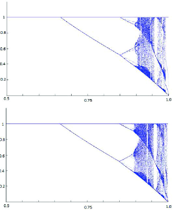
Figure 4: Feigenbaum diagram for the process on four coordinates (top) and five coordinates (bottom).

The Feigenbaum diagrams for $n=4$ and $n=5$ are similar to the diagram for $n=3$, and as it turns out that this holds in general for all $n>3$. The main difference between $n=3$ and $n>3$ is the appearance of a chaotic region for $0.95<\theta<1$. It is remarkable that a stable point of period three reappears around $\theta\approx 0.95$. For $n=4$ the stable cyclic point of period four appears at $\theta\approx 0.99$ and is still visible in this figure. For $n=5$ it appears only at $\theta\approx 0.999$ and it is not visible in this picture. To show that our analysis holds and that the periodic point does exist, we zoom in on step sizes in $(0.95,1)$ in the next figure.

Figure 5: Feigenbaum diagram for the process on five coordinates: zoom in on $\theta\geq 0.95$.

The diagram shows the cyclic period five for $\theta$ near $1$. This concludes our analysis of the Dikin process $w^{k}$. Now to prove that this analysis makes sense, we still need to check that the primal-dual AFS method displays the same type of chaotic behavior as $w^{k}$. We will do that in the next and final section.

VI Comparison to primal-dual AFS

The iterative process $w^{k}$ has been derived by a linearization of the primal-dual AFS method. To show that our bifurcation analysis bears any relevance, we need to verify that a simlar route to chaor occurs in actual LO problems. There is one complication. The Dikin process involves a parameter $\theta$ that defines the step-size with respect to the maximum $\alpha_{max}=\frac{\|xs\|}{\max{xs}}$. So if we consider the primal-dual AFS method, then we should set our step size accordingly. This means that $\alpha$ should not be constant, which it is in the original primal-dual AFS method, but we should take it to be equal to $\theta\alpha_{\max}$. We modify the AFS method in this way and we put $\alpha=\theta\alpha_{max}$.

We take the same example as considered by Castillo and Barnes in Barnes :

$$\begin{matrix}\min{10x_{1}+10x_{2}+5x_{3}+x_{4}-x_{5}}\\ \text{under the constraints}\\ x_{1}+2x_{2}-3x_{3}-2x_{4}-x_{5}=0\\ -x_{1}+2x_{2}-x_{3}-x_{4}-x_{5}=0\\ x\geq 0\end{matrix}$$ (15)

We take the same initial vectors $x_{0}$ and $y_{0}$ as Castillo and Barnes and run our modified primal-dual AFS method that we describe in pseudo-code below. The numerical task of computing the limit of the AFS process is not trivial, especially for a larger values of the step size, because $x^{k}$ rapidly converges to zero which leads to numerical problems, caused by inverting matrices that are ill conditioned. Castillo and Barnes developed analytic formulas that enabled them to still compute Feigenbaum diagrams with high precision. Such an analytic exercise is beyond the scope of our paper. We stop the computation once the duality gap reaches $10^{-10}$.

 

Modified Primal–Dual AFS

 

Parameters

$\varepsilon$ is the accuracy parameter;

$\theta$ is the scaled step size;

Input

$(x^{0},s^{0})$: the initial pair of interior feasible solutions;

begin

$x:=x^{0};\,s:=s^{0}$;

while $x^{T}s>\varepsilon$  do $w=xs$;

$\alpha_{max}=\frac{\|w\|}{\max w}$;

$\alpha=\theta\alpha_{max}$;

$x:=x+\alpha\Delta x$;

$y:=y+\alpha\Delta y$;

$s:=s+\alpha\Delta s$;

end.

 

Figure 6: Primal–dual affine scaling algorithm with modified step size $\alpha$. In our computations we put $\varepsilon=10^{-10}$ and we plot results as soon as the duality gap reaches values $\leq 0.001$

We have computed the Feigenbaum diagram for the scaled process $\frac{w^{k}}{\max w^{k}}$ that is given in Figure 7. The diagram below depicts the limit of the fourth coordinate. There is a bifurcation for $\theta=2/3$ and another bifurcation close to $\theta=0.86$, followed by a chaotic regime. At the end of the diagram, for values of $\theta$ close to $1$, we find a stable periodic point. This is similar to the diagrams that we computed earlier for our process $w^{k}$, although the periodic point at the end of the diagram is period three instead of period five. The Feigenbaum diagram above, which depicts the second coordinate, shows a different picture. The diagram bifurcates at $\theta=2/3$ but the two branches of the graph intersect twice between $2/3$ and $0.86$: once at $\theta\approx 0.69$ and once at $\theta\approx 0.78$. At these values of $\theta$, the limit lands exactly on the unstable fixed point. We already noticed that this point is weakly repelling, which is why the second coordinate has not yet fully converged to its $\omega$-limit yet, even when the duality gap is $10^{-10}$.

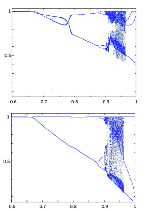
Figure 7: Feigenbaum diagrams for the Castillo-Barnes LO problem. Horizontal coordinate represents $\theta$. Vertical axis contains the $\omega$-limit of a coordinate of the scaled vector $w$. Second coordinate above. Fourth coordinate below.

The dual problem is degenerate

$$\begin{matrix}\max{0}\\ \text{under the constraints}\\ y_{1}-y_{2}\leq 10\\ 2y_{1}+2y_{2}\leq 10\\ -3y_{1}-y_{2}\leq 5\\ -2y_{1}-y_{2}\leq 1\\ -y_{1}-y_{2}\leq-1\end{matrix}$$ (16)

All feasible points solve the dual problem. If $\theta\leq 2/3$ then the process $y^{k}$ converges to $(3.0513,0.5522)$ but if $\theta$ increases beyond $2/3$ then the process no longer converges to a single point. However, $y^{k}$ remains within the feasible set even for large values of $\theta$. Figure 8 contains the limit set that we computed for $\theta=0.94$. It has the contours of a Hénon-like strange attractor. The image of the attractor is slightly blurred since the orbit has not fully converged yet.

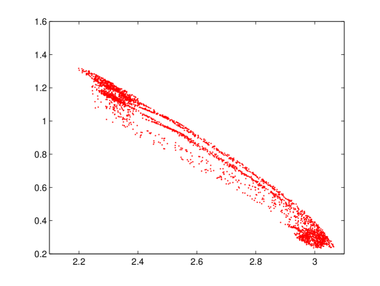
Figure 8: The omega-limit set of the vector $y$ in the dual problem for $\theta=0.94$ forms a strange attractor in the feasible set.

It seems that the process $w^{k}$ that we have considered in this paper represents the iterations of primal-dual AFS rather well. We have tested other LO problems as well and we find similar Feigenbaum diagrams for the vector $w$, regardless whether the dual problem is degenerate or not. The algorithm converges to an optimal solution for relatively high values of $\theta$, so for a step-size that is close to $\alpha_{max}$. This may indicate that a step-size that is larger than $1/(15\sqrt{n})$ is possible, if $\alpha$ is not taken to be constant but is allowed to vary with $xs$, as in our computations.

VII Conclusion

We have presented the Dikin process as an archetype for general interior point methods. The Dikin process is a one-parameter family with a route to chaos that bears similarity to the the logistic family, and which agrees with the chaotic behaviour of interior point methods that has been previously observed.

References

- (1) B. Jansen, C. Roos, T. Terlaky. A polynomial Dikin–type primal–dual algorithm for linear programming. Mathematics of Operations Research, 21:341–353, 1996.
- (2) I. Castillo, E. R. Barnes. Chaotic behavior of the affine scaling algorithm for linear programming. SIAM Journal on Optimization, 11 (3), 781–795, 2000.
- (3) N. K. Karmarkar. A new polynomial–time algorithm for linear programming. Combinatorica, 4:373–395, 1984.
- (4) S. J. Wright. Primal-Dual Interior-Point Methods. SIAM, Philadelphia, 1996.
- (5) Y. Ye. Interior Point Algorithms, Theory and Analysis. John Wiley & Sons, Chichester, UK, 1997.
- (6) R. J. Vanderbei. Linear Programming: Foundations and Extensions. Kluwer Academic Publishers, Boston, USA, 1996.
- (7) C. Roos, T. Terlaky, J.-Ph. Vial. Interior point methods for linear optimization. Springer, New York, 2006. Second edition of Theory and algorithms for linear optimization [Wiley, Chichester, 1997; MR1450094].
- (8) R. J. Vanderbei, M. S. Meketon, B. A. Freedman. A modification of Karmarkar’s linear programming algorithm, Algorithmica, 1, 395–407, 1986.
- (9) T. Tsuchiya, M. Muramatsu. Global convergence of a long-step affine scaling algorithm for degenerate linear programming problems. SIAM Journal on Optimization, 5:525–551, 1995.
- (10) L. A. Hall, R. J. Vanderbei. Two-thirds is sharp for affine scaling. Oper. Res. Lett., 13 no.4 (1993), 197–201.
- (11) W. F. Mascarenhas. The affine scaling algorithm fails for stepsize 0.999, SIAM Journal on Optimization, 7(1):34–46, 1997.
- (12) I. I. Dikin. Iterative solution of problems of linear and quadratic programming. Doklady Akademii Nauk SSSR, 174:747–748, 1967. Translated in: Soviet Mathematics Doklady, 8:674–675, 1967.
- (13) M. J. Feigenbaum. Quantitative universality for a class of nonlinear transformations. J. Stat. Phys., 19(1): 25–53, 1978.
- (14) G. Eneström. Härledning af en allemän formel för antalet pensionärer. Ofv. af Kungl. Vetenskaps Akademiens Förhandlingar 6, 1893.