Identification of
Influential Scientists vs. Mass Producers
by the Perfectionism Index
Abstract
The concept of h-index has been proposed to easily assess a researcher’s performance with a single number. However, by using only this number, we lose significant information about the distribution of citations per article in an author’s publication list. In this article, we study an author’s citation curve and we define two new areas related to this curve. We call these “penalty areas", since the greater they are, the more an author’s performance is penalized. We exploit these areas to establish new indices, namely PI and XPI, aiming at categorizing researchers in two distinct categories: “influentials" and “mass producers"; the former category produces articles which are (almost all) with high impact, and the latter category produces a lot of articles with moderate or no impact at all. Using data from Microsoft Academic Service, we evaluate the merits mainly of PI as a useful tool for scientometric studies. We establish its effectiveness into separating the scientists into influentials and mass producers; we demonstrate its robustness against self-citations, and its uncorrelation to traditional indices. Finally, we apply PI to rank prominent scientists in the areas of databases, networks and multimedia, exhibiting the strength of the index in fulfilling its design goal.
1 Introduction
The h-index has been a well honored concept since it was proposed by Jorge
Hirsch [16]. A lot of variations have been proposed in the
literature, see for instance the references within [1].
Many efforts enhanced the original h-index by taking into account
age-related issues [27],
multi-authorship [18], fractional
citation counting [20], the highly cited
articles [12]. Other works explored its
predictive capabilities [17], its robustness to
self-citations [26], etc. Some of the proposals
have been implemented in commercial and free software, such as
Matlab111http://www.mathworks.de/matlabcentral/fileexchange/28161-bibliometrics-the-art
-of-citations-indices
and the Publish or Perish software 222http://www.harzing.com/pop.htm.
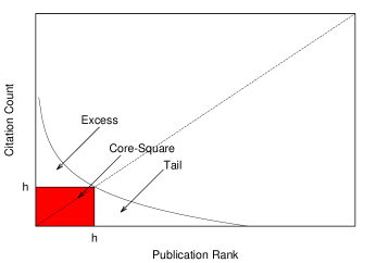
Even though there are several hundreds of articles developing variations to the original h-index, there is notably little research on making a better and deeper exploitation of the “primitive" information that is carried by the citation curve itself and by its intersection with the line defining the h-index. The projection of the intersection point on the axes creates three areas that were termed in [25], [31], and [32] as the h-core-square area333In the sequel of the article for the sake of simplicity, we use the term h-core and h-core-square interchangeably. , the tail area and the excess area (see Figure 1). The core area is a square of size (depicted by grey color in the figure), includes citations and it is also called Durfee square area [2]; the area that lies to the right of the core area is the tail or lower area, whereas the area above the core area is the excess or upper or area [32]. Both the absolute and the relative sizes of these areas carry significant information. The absolute size of the excess and core areas were directly used for the definition of e-index and h-index; part of the absolute size of the tail area was used in [15] to create a vector of h-indices; the relative size of the core to the tail area (without taking into account the tail length) was used in [31] for similar purposes, etc. ( For a complete review of the relevant bibliography cf. section 2.) The common characteristic of all these works is that they develop indices to “break ties", i.e., to differentiate between scientists with equal h-indices, and thus address the isohindex problem.
We believe that the latent information carried by these areas is not adequately explored, and most significantly, it can be used in a different way, not as a plain tie-breaker, but as a “first-class" citizen in the scientometric indices ecosystem.
Rosenberg [24] took the first step towards this goal; he provided a qualitative characterization for the scientists with many citations in the upper area and a few citations in the tail area by referring to them as perfectionists. He referred to the authors with few citations in the upper area and many citations in the tail area as mass producers, since they have a lot of publications but mostly of low impact. Finally, he referred to the rest of the scientists as the prolific ones. The origin of this terminology is quite old; it was proposed in [9], and subsequently studied further in [13].
Motivated by Rosenberg’s classification scheme, we pose the following question: “Can we develop a quantitative methodology for identifying those scientists who are truly “laconic" and constantly influential compared to those who produce a mass of papers but relatively few of them contribute to their h-index?"
In the present paper, we will present a methodology and an easy calculated criterion to categorize a scientist in one of two distinct categories: either an author is a “mass producer", i.e., he has authored many papers with relatively few citations or he is “influential", i.e., most of his papers have an impact because they have received a significant number of citations. This methodology will indirectly highlight the “attitude" towards publishing. Some scientists are acting in a laconic way, in the sense that they are not fond of having published “half-baked" articles that are soon superseded by mature and extended versions of their work. Others develop their work in a slow and incremental way, publishing their ideas in a step-by-step fashion producing a lot of moderate impact articles until they hit the big contribution. This attitude may be due to other reasons as well, e.g., the pressure to present published articles as deliverables to a project. In any case, it is not the purpose of the present article to discover and explain those reasons. The sole purpose of our work is to develop metrics that can be used complementary to the traditional ones such as the h-index, in order to separate the steadily influential authors from the mass producers. At this point we need to emphasize that the concept of “influential" scientists we develop here is not related to the notion of influential nodes in a social network of actors as considered in [3].
The area of scientometric performance indicators is very rich, and it is continuously flourishing. Vinkler in [30] provides a brief classification of the traditional and modern scientometric indicators explaining their virtues and shortcomings; it is shown there that Hirsch index is not the only indicator that combines impact and quantity, but -index [29] which introduced the concept of “elite set" is another competitor of it. Nevertheless, in this article we use Hirsch index as a basis to expose our ideas claiming that neither Hirsch index is the ’best’ one nor that our core methodology applies exclusively to it. We are strongly confident that our ideas can be applied also to the family of indices based on the Impact Factor by penalizing those journals that publish articles which accumulate far less citations than the Impact Factor of the journal they appear in.
The rest of the article is organized as follows. In the next section we will present the relevant literature and then define two new areas in the citation curve. Based on these two new areas, we will establish two new metrics for evaluating the performance of authors in terms of impact. In Section 4 we will present our datasets, which were built by extracting data from the Microsoft Academic Search database, and analyze these data to view the dataset characteristics. Subsequently, we will present the distributions of our new metrics for the above datasets and compare them with other metrics proposed in the literature. Finally, in Section 5 we will present some of the resulting ranking tables based on the new metrics and h-index. Section 6 will conclude the article.
1.1 Motivation and contributions
During the latest years an abundance of scientometric indices have been published to evaluate the academic merit of a scientist. Despite the debate around the usefulness of any index in general, they remain an indispensable part of the evaluation process of a scientist’s academic merit. The ideas behind the h-index philosophy was so influential, that the vast majority of the proposed indices are about some variant or extension of the h-index itself. Despite the wealth and sophistication of the proposed indices, we argue that the relevant literature did not strive for an holistic consideration of the information carried by the citation curve and by the line. In the next paragraph we will present the motivating idea with a simple example.
Let us consider author who has published 13 articles, and author who has published 24 articles with citation distributions and respectively. Both authors have the same “macroscopic" characteristics in terms of the number of citations, i.e., they both have the same total number of citations, identical core areas and h-indices equal to 10, identical excess areas with 65 citations there, and the same number of citations in the tail area, namely 12. However, author has only 3 articles in his tail area, whereas author has 14 articles.
At a first glance, we can simply use the number of articles in the tail as a tie-breaker to differentiate between the two authors, and characterize the first one as constantly “influential", and the second one as a “mass producer". But, how can we capture the fact that, in the short term, the first author’s h-index is more likely to increase. At the same time, we need a way to describe – actually, to penalize – the second author for this long and lightweight tail. Starting from these questions we will define the penalty areas and then develop the respective indices. In this article, we do not consider temporal issues, e.g., the time of publication of the articles in the tail area; such issues are part of our on-going work. Specifically, the article makes the following contributions:
-
•
It defines two areas to quantify the fact that some authors publish articles which eventually do not have analogous impact with those that contribute to their h-index.
-
•
It develops two new perfectionism indices taking into account the size of the penalty areas. There are the and indices, which are statistically uncorrelated to the h-index, thus proving that they measure something that is different from what the h-index measures.
-
•
Using these indices, it proposes a filter to separate the authors into influential ones and mass producers. This filter partitions the authors irrespectively of their h-index, i.e., it can classify two authors as influentials, even if the values of their h-indices are significantly different. This two-way segmentation of the scientists is a significant departure from the earlier, rich classification schemes [9, 13], since with a single integer number and its sign (plus or minus) it can provide rankings, contrary to intuitive mapping schemes such as that in [34].
-
•
It provides a thorough investigation of the indices against the h-index for three datasets retrieved by the Microsoft’s Academic Search.
At this point, we need to emphasize again that the proposed indices are neither a substitute for any of the already existing metrics nor a tool for identifying “bad" publishing behaviour. They are one more tool in the indices toolbox of someone who wishes to capture the multi-dimensional facet of a scientist’s performance.
2 Relevant work
The original article by Hirsch [16] created a huge wave of proposals for indices attempting to capture the academic performance of a scientist. It is characteristic that at the time of writing the present article, the h-index’s article had more than 3850 citations in Google Scholar. Since the focus of the present manuscript is not about the h-index in general, but about the exploitation of the information in the tail area, we will survey only the articles relevant to the usage and mining of that part of the citation.
Ye and Rousseau [31] studied the evolution of tail-core ratio as a function of time, and later extended their study in [22] including a few more ratios among the three areas. Similar in spirit is the work reported in [7], which examines variations of the ratios across scientific disciplines. Baum [4] introduced the ratio (the relative citedness) of the few, highly-cited articles in a journal’s h-core and the many, infrequently-cited articles in its h-tail as a way to improve journals’ Impact Factors.
Having as motive to consider each and every citation under the whole citation curve (and therefore under the tail area as well) , Anderson et al. [2] proposed a fractional citation counting scheme based on Ferrers graphs. Later, Franceschini and Maisano [14] recognized the weaknesses of that scheme and proposed the Citation Triad method; both indices are striving to exploit the information under the whole citation curve in a way that creates a strictly monotonic (increasing) index for every new citation added to the curve, which is completely different to what we propose.
A kind of “quantization" scheme for the citation curve and the creation of multiple Durfee squares under that curve was proposed in [15]. The output of that method was a vector (i.e., multiple h-indexes) as a measure of the scientific performance. However, the method simply transformed the task of comparing different citation curves into the problem of comparing vectors, without setting clear rules. A study of the contribution of the excess, core and tail areas to the entire citation curve was performed in [5] proving that this contribution varies across scientists. The study provided also a regression model for determining the most visible article of a scientist. The position of the centroids of the core and tail area was used in [21] as an index for comparing different scientists providing only straightforward characterizations for high-low impact and productivity. Along these lines of research, Zhang [34] proposed a triangle mapping technique to map the three percentages (of the excess, core and tail area) of these citations onto a point within a regular triangle; by viewing the distribution of the mapping points, different shapes of citation curves can be studied in a perceivable form. The work described in [11] sought selective and large producers considering only a part of the excess and a part of the tail area, thus again neglecting a part of the tail area which carries significant information.
The most closely relevant articles to our work are [24] and [33]. Rosenberg [24] described a three-class scheme for scientists’ classification based on the length and thickness of the tail of the citation curve. Zhang in [33] proposed the index as a quantitative measure to discover which scientist belongs to which one of those three categories.
Collectively, the present work differentiates itself by the previous studies in a number of factors: a) it exploits the full spectrum of information under the citation curve, b) it is based on the definition of new areas (not below, but above the citation curve), c) it penalizes those scientists with long and thin tails, d) it proposes an index that can be used as a filter to separate the constantly influential scientists from the mass producers.
3 Penalty areas and the Perfectionism Indices
In this section, we will define the penalty areas which form the basis for the development of the respective scientometric indices. Before proceeding further, we summarize in Table 1 some symbols, their interpretations, and the relationships among them, which will be used throughout this article.
| Symbol | Description | Relations |
|---|---|---|
| h-index of an author | ||
| number of articles of an author | ||
| set of articles of an author | ||
| set of articles that belong in the core area | ||
| set of articles that belong in the tail area | ||
| number of articles that belong in | ||
| number of citations of an author | ||
| number of citations for publication | ||
| number of citations for publications in | [19] | |
| number of citations for publications in | ||
| number of citations in the upper (excess) area |
3.1 The tail complement penalty area
We now get back to the motivating example presented in the previous section, and we illustrate graphically their citation distributions (see Figure 2). We depict with red color the h-core area of each author.
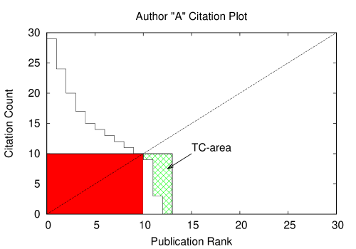
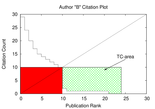
It is intuitive that long tails and light-weight tails reduce an author’s articles’ collective influence. Therefore, we argue such kind of a tail area should be considered as a “negative" characteristic when assessing a scientists’s performance. The closer the citations of the tail’s articles get to the line , the more probable it is for the scientist to increase his h-index, and at the same time to be able to claim that practically each and every article he publishes does not get unnoticed by the community.
For this purpose, we define a new area, the tail complement penalty area, denoted as TC-area with size . The size of the tail complement penalty area is computed as follows:
| (1) |
This area is depicted with the green crossing-lines pattern in Figure 2, and fulfilling the motivation behind its definition, it is much bigger for author than for author .
3.2 The ideal complement penalty area
If we push further the idea of the tail complement penalty area, we can think that “ideally" an author could publish papers with citations each and get an h-index equal to . Thus, a square could represent the minimum number of citations to achieve an h-index value equal to . Along the spirit of penalizing long and thin tails, we can define another area in the citation curve: the ideal complement penalty area (IC-area), which is the complement of the citation curve with respect to the square . Figure 3 illustrates graphically the IC-area with the green crossing-lines pattern. The size of the IC-area () can be computed as follows:
| (2) |
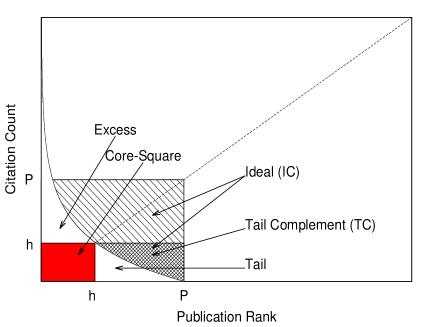
Apparently, this area does not depend on the h-index value, as it holds for the case of the TC-area. Notice that the IC-area includes the TC-area defined in the previous paragraph. We realize of course that it is hard (if possible at all) to find scientists – with sufficiently large h-index, and – with zero-sized TC-area, since citation distributions approximately follow power laws [6, 8, 23]. Therefore, the index derived by this area is not expected to provide significant insights into scientists’ performance.
3.3 The new scientometric perfectionism indices: and
The definition of the penalty areas in the previous subsection, allows us to design two new metrics which will act as the filter to separate influential from mass producers. Firstly, let us introduce the concept of Parameterized Count, , as follows:
| (3) |
where are integer values. Apparently:
-
•
when , then it holds that ,
-
•
when , then ,
-
•
when , then ,
-
•
when , then .
By assigning positive values to and , but negative values to , we can favor authors with short and thick tails in the citation curve. Even in this way, we cannot differentiate between the authors and of our example.
For this reason, instead of using the tail of the citation curve, we use the tail complement penalty area. Thus, similarly to Equation 3, we define the concept of Perfectionism Index based on TC-area as follows:
| (4) |
In the experiments that will be reported in the next sections, we will use the values of . These default values give a straightforward geometrical notion of the newly defined metric. Noticeably, it will appear that can get negative values. Thus:
-
•
if an author has , then we characterize him as a mass producer,
-
•
if an author has , then we characterize him as an influential.
In the same way as the ’s definition, we define an extremely perfectionism metric, the Extreme Perfectionism Index, taking into account the ideal complement penalty area, as follows:
| (5) |
As in the previous case, we will assume that . We will show in the experiments, that very few authors have positive values for this metric. Using the previously defined perfectionism indices, the resulting values for authors and are shown in Table 2. Author has greater values than author for both and perfectionism indices. This is a desired result.
| Author | ||||||||||
|---|---|---|---|---|---|---|---|---|---|---|
| 13 | 177 | 10 | 12 | 65 | 165 | 18 | 147 | 33 | 144 | |
| 24 | 177 | 10 | 12 | 65 | 165 | 128 | 37 | 404 | -227 |
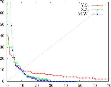
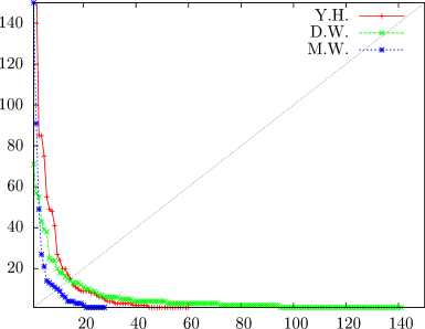
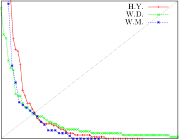
Before proceeding to the next section, which describes the detailed experiments that demonstrate the merits of the new indices, we provide an additional example of five authors with different publishing patterns, as an extension to our artificial motivating example which was presented in the beginning of the article. We use only initials but they refer to real persons and their data. In Table 3 we present the raw data (i.e., h-index, number of publications and number of citations ) of 5 authors444We selected authors with relatively small number of publications and citations for better readability of the figures. selected from Microsoft Academic Search555http://academic.research.microsoft.com/. The last column shows the calculated values, which can be positive as well as negative numbers. In Figure 4 we present citation plots for these five authors.
In Figure 4 we compare three authors: S.Y., Z.Z. and W.M. They all have an h-index equal to 10. Note that S.Y. has a comparatively large number of publications but the citation curve is cropped to focus on the lower values. As he has the bigger and longest tail (red line), he could be characterized as a “mass producer". This is reflected in a value of as shown in Table 3. Z.Z. (green line) has shorter tail than S.Y. and higher excess area. From the same table we remark that his value is 11 (i.e. close to zero). Finally, the last author of the example, W.M. (blue line), has similar tail with Z.Z. but a bigger excess area (). Definitely, he demonstrates the “best" citation curve out of the three authors of the example. In fact, his score is 717, higher than the respective figure of the other two authors.
| Author | ||||
|---|---|---|---|---|
| H. Y. | 15 | 105 | 2040 | 690 |
| W. D. | 15 | 259 | 1137 | -2523 |
| W. M. | 10 | 48 | 1097 | 717 |
| S. Y. | 10 | 319 | 585 | -2505 |
| Z. Z. | 10 | 49 | 391 | 11 |
In Figure 4, again we compare three authors: H.Y., W.D. and W.M. The first two have h-index value equal to 15. Comparing those, it seems that H.Y. (red line) has a better citation curve than W.D. (green line) because he has a shorter tail and a bigger excess area. Indeed, the first one has , whereas the second one has . W.M. (blue line) has a smaller tail and a big excess area but since there is a difference in h-index we cannot say for sure if he must be ranked higher or not than the others.
In Figure 4(a) we have scaled the citation plots so that all lines cut the line at the same point. From this plot, it is shown that W.M. has a better curve than W.D. because he has a shorter tail and a bigger excess area. When comparing W.M. to H.Y., we see that the latter has a longer tail but also a bigger excess area. Both curves show almost the same symmetry around the line . That is why they both have similar values. This is a further positive outcome as authors with different quantitative characteristics (say, a senior and a junior one) may have similar qualitative characteristics, and thus be classified together.
4 Experiments
In this section, we will present the results of the evaluation of the proposed indexes. The primary goal of our experimentation is to study the merits of the index, since our results confirmed that the severe penalty that imposes makes it a less useful scientometric tool. Firstly, we will explain the procedures for dataset acquisition, then we will present their characteristics, and finally we will give the results that concern the evaluation of .
4.1 Datasets acquisition and characterization
During the period December 2012 to April 2013, we compiled 3 datasets. The first one consists of randomly selected authors (named “Random" henceforth). The second one includes highly productive authors (named “Productive"). The last one consists of authors in the top h-index list (named “Top h"). The publication and the citation data were extracted from the Microsoft Academic Search (MAS) database using the MAS API.
The dataset “Random" was generated as follows: We fetched a list of about 100000 authors belonging to the “Computer Science" domain as tagged by MAS. MAS assigns at least three sub-domains to every author. These three sub-domains may not all belong to the same domain (e.g., Computer Science). For example, an author may have two sub-domains from Computer Science and one from Medicine. We kept only the authors who have their first three sub-domains belonging to the domain of Computer Science. From this set, we randomly selected 500 authors with at least 10 publications and at least 1 citation.
The dataset “Productive" was generated as follows: from the set of 100000 Computer Science authors we selected the top-500 most productive. The least productive author from this sample has 354 publications.
The third dataset named “Top h" was generated by querying the MAS Database for the top-500 authors in the “Computer Science" domain ordered by h-index.
Table 4 summarizes the information about our datasets with respect to the number of authors (line: # of authors), number of publications (line: # of publications), number of citations (line: # of Citations) and average/min/max numbers of citations and publications per author.
| Random | Productive | Top h | |
|---|---|---|---|
| # of authors | 500 | 500 | 500 |
| # of publications | 25679 | 223232 | 149462 |
| #P/Author | 51 | 446 | 298 |
| Min #P/Author | 10 | 354 | 92 |
| Max #P/Author | 768 | 1172 | 1172 |
| # of Citations | 410280 | 3197880 | 5015971 |
| # Cit/Author | 820 | 6395 | 10031 |
| Min #Cit/Author | 1 | 25 | 4405 |
| Max #Cit/Author | 47263 | 47263 | 47263 |
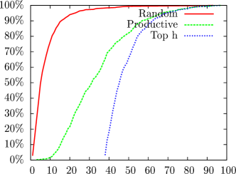
Figure 5 shows the distributions for the values of h-index, , and . The index was defined in Hirsch’s original article [16] and is explained (quoting Hirsch’s text) in the next paragraph. Plots are illustrated in pairs. The ones on the left show cumulative distributions. For example, in Figure 5(a) we see that 80% of the authors in the sample “Random" (red line) have h-index less than 10. It is obvious that the sample “Top h" (blue line) has higher values for the h-index. Figures 5(c) and 5(d) show the distributions for the total number of citations. As expected the sample “Top h" has the highest values.
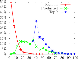
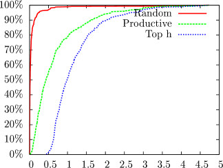
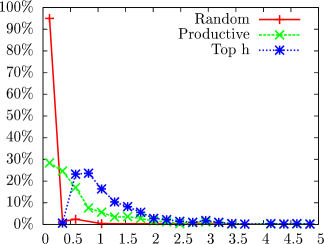
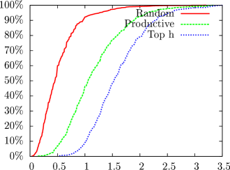
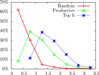
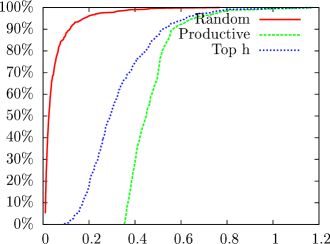
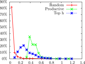
Figures 5(e) and 5(f) show the distributions for the value. Recall its definition from [16]: A value of (i.e., an h-index of 20 after 20 years of scientific activity), characterizes a successful scientist. A value of (i.e., an h-index of 40 after 20 years of scientific activity), characterizes outstanding scientists, likely to be found only at the top universities or major research laboratories. A value of or higher (i.e., an h-index of 60 after 20 years, or 90 after 30 years), characterizes truly unique individuals. Indeed, only a few authors have .
Figures 5(g) and 5(h) illustrate the distributions for the total number of publications. It is obvious that in the “Random" sample (red line) there are relatively low values for the total number of publications. Also, as expected, the distribution for the “Productive" sample has the highest values for the total number of publications.
4.2 Does offer new insights about the impact and publication habits of scientists?
The first question that needs to be answered is whether a new index offers something new and different compared to the existing (hundreds of) indices. The answer is positive; our metric separates the rank tables into two parts independently from the rank positions.
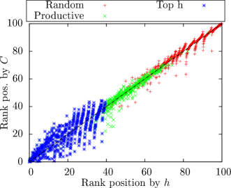
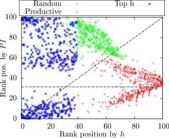
In Figure 6(a) the x-axis denotes the rank position (normalized percentagewise) of an author by h-index, whereas the y-axis denotes the rank position by the total number of citations (). Each point denotes the position of an author ranked by the two metrics. Note that all three samples are merged but if the point is blue, then the author belongs to the “Top h" sample, if the point is green then he belongs to the “Productive" sample etc. If an author belongs to more than one sample, then only one color is visible since the bullet overwrites the previous one. From Figure 6(a) the outcomes are:
-
•
“Top h" authors are ranked in the first 40% of the rank table by h-index, as well as in the top 40% by the total number of citations ().
-
•
“Productive" authors are mainly ranked by h-index between 30% and 70%. The rank positions by are between 20% and 70%.
-
•
“Random" authors are mainly ranked below 60% for both metrics with some outliers in the range 0-60%, mostly by .
The aforementioned conclusions are as expected; it also occurs that h-index ranking does not differ significantly from the ranking; i.e., they are correlated which is consistent666http://michaelnielsen.org/blog/why-the-h-index-is-virtually-no-use/ with earlier findings [28].
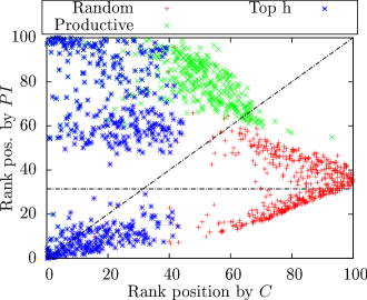
In Figure 6(b) the h-index ranking is compared to ranking. It can be seen that there is no correlation between and h-index. Note that the horizontal line at about 32% (also shown later in Table 5) shows the cut point of for the zero value. Authors that reside below this line have and authors above this line have .
-
•
“Top h" authors are split to two groups. The first group is ranked in the top 20% of the rank table. The second group is ranked in the last 50%. These two groups are also separated by the zero line of .
-
•
“Productive" authors are almost all ranked at lower positions by than by h-index. Almost all points reside above the zero line and also above the line (with some exceptions at about 65-70% of the rank list).
-
•
“Random" authors are also generally higher ranked by than by h-index. They are also split into two groups by the line .
From the above, it seems that is not correlated to h-index, whereas the line plays the role of a symmetric axis. Thus, it emerges as the key value that separates the “influential" authors from the “mass producers".
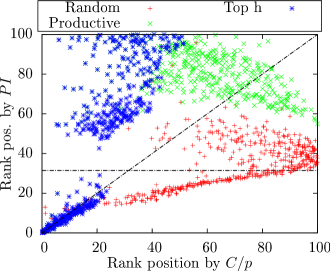
In Figure 6(c) we compare ranking against (total number of citations) ranking. It is expected that the plot would be similar to Figure 6(b) based on the similarity of h-index with .
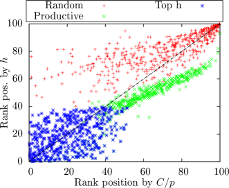
In Figures 6(d) and 6(e) we compare h-index and with the average number of citations per publication () ranking. It is apparent that is not correlated to . h-index is also uncorrelated to , however the points of the qq-plot in Figure 6(e) are closer to the line than the points of Figure 6(d).
Conclusively, the ranking is not correlated to h-index, and .
4.3 Aggregate analysis of the datasets
Figure 7 shows the distributions for the areas defined in the previous section. In particular, Figures 7(a) and 7(b) illustrate the distributions for the (tail) area. It seems that the “Top h" cumulative distribution is very similar to the “Productive" one, however, the “Top h" distribution has slightly higher values.
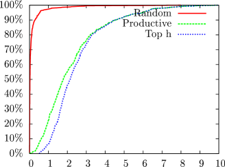
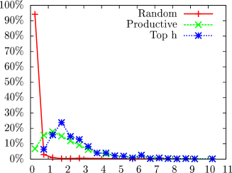
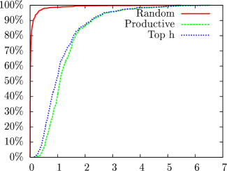
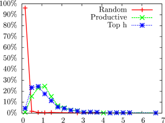
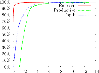
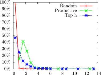
Figures 7(c) and 7(d) illustrate the distributions for the (tail complement) area. It seems that has the same distribution as for all samples except for the sample “Productive", for which has slightly higher values than does. Note, also, that the “Productive" distribution has lower values for h-index than “Top h". This means that the height of the areas is smaller for the “Productive" authors than for “Top H’ ones. The previous two remarks lead to the (rather expected) conclusion that the “Productive" authors have long and thin tails.
The distribution is shown in Figures 7(e) and 7(f). In these plots, it is clear that the “Productive" authors have clearly higher values than any other sample, since is strongly related with the total number of publications.
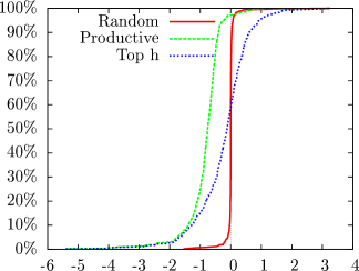
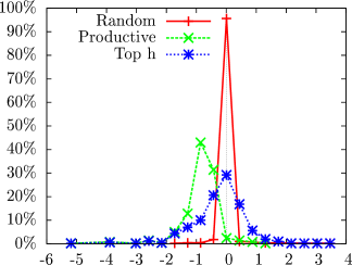
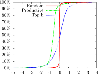
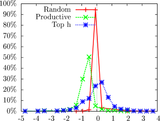
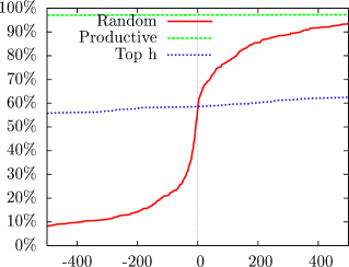
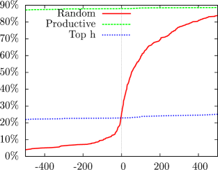
In Figure 8 we see the distributions for the previously defined index. Interestingly, it seems that the value 0 is a key value. For all plots, the zero y-axis is the center of the figure. As seen in Figures 8(a) and 8(b) most of the authors are located around zero. Note that in the right plots, a point at with a previous value of means that the 95% of the authors have values in the range . The first two plots show that the “Top h" authors have the highest values for (about 10% of them have values greater than 8000).
Figure 8(g) is a zoomed-in version of Figure 8(a). It is clear that about 96% of the “Productive" authors have . This means that in this sample there are a lot of “mass producers" (people with high number of publications but relatively low h-index- or at least not in “Top h-indexers"). The other samples cut the zero y-axis at about 50% to 60%, which means that 40% to 50% are positive. It is also noticeable that about 70% (15-85%) of the “Random sample have values very close to zero within the range -200..200.
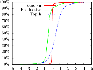
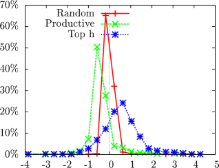
In Figure 8(c), 8(d), 8(e) and 8(f) we present the distributions for and . We remind that factor is the core area multiplier. In these plots, it is shown that these distributions behave like the basic distribution except that they are slightly shifted to the right. The "Productive" sample is affected less than the others. This outcome is understandable since they are the authors with small h-index core areas compared to their tail and excess areas.
Comparing subfigure 8(h) to 8(g) we can better see the differences. The number of authors in the negative side of samples “Random" and “Top h" has decreased from 57% and 58% to 24% and 23% respectively, meaning that about 33%-35% of the sample members moved from the negative to the positive side. The number of “Productive" authors in the negative side has been decreased from 97% to 88%, i.e. an additional 11% of the sample members moved to the positive side.
In addition to the distribution plots, Table 5 presents the number of authors that have the mentioned metrics below or above zero for each sample. As mentioned before, 97% of the “Productive" authors have , whereas only 3% reside in the positive side of the plot. This amount increases as we increase the core factor . For the increment is 9% (12% from 3%). In all other samples the increment is greater, i.e. for “Top h" the increment is 35%, for “Random" is 33%.
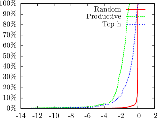
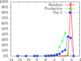
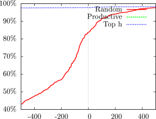
In Figure 9 the same kinds of plots are presented for the metric . As expected, the difference is that most of the authors lie in the negative side of the graph. The cut points of y-axis are also presented in Table 5. About 2% of the “Top h-index " authors have but none of the “Productive" authors do. The cut point for “Random" authors is at 6%. Also, at this point we repeat the experiment of varying the value. The results do not match with those of the case. Incrementing does not increase the number of positive authors in the same way as the case. The increment is negligible for the “Productive" and “Top h" and very small for the sample “Random". This leads to the conclusion that varying the factor does not affect significantly. Probably different default values for the factors of Equation 4 (especially for and/or ) may be needed for tuning the metric. However, this task remains out of the scope of the present article.
| Sample | ||||||||||||
|---|---|---|---|---|---|---|---|---|---|---|---|---|
| Random | 284 | 216 | 213 | 287 | 122 | 378 | 418 | 82 | 408 | 92 | 383 | 117 |
| 57% | 43% | 43% | 57% | 24% | 76% | 84% | 16% | 82% | 18% | 77% | 23% | |
| Productive | 485 | 15 | 474 | 26 | 439 | 61 | 500 | 0 | 500 | 0 | 500 | 0 |
| 97% | 3% | 95% | 5% | 88% | 12% | 100% | 0% | 100% | 0% | 100% | 0% | |
| Top | 292 | 208 | 226 | 274 | 114 | 386 | 488 | 12 | 484 | 16 | 473 | 27 |
| 58% | 42% | 45% | 55% | 23% | 77% | 98% | 2% | 97% | 3% | 95% | 5% | |
| Unioned | 904 | 419 | 767 | 556 | 563 | 760 | 1230 | 93 | 1216 | 107 | 1180 | 143 |
| 68% | 32% | 58% | 42% | 43% | 57% | 93% | 7% | 92% | 8% | 89% | 11% | |
4.4 robustness to self-citations
Self-citations (a citation from an article to another article when there is at least one common author between the citing and the cited paper) is a common way for authors to increase the visibility of their works; it has significant impact on h-index [26], and some efforts has been made towards designing robust metrics to self-citations [20].
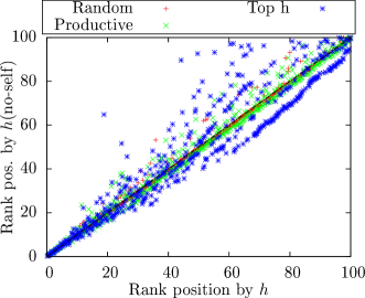
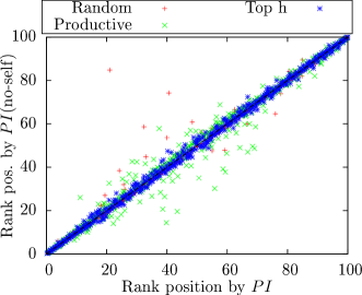
We performed an experiment to study the behavior of h-index and PI with respect to self-citations. In Figure 10(a) a qq-plot is shown, which compares the ranking produced by h-index. The x-axis represents the rank produced by the computed h-index including self-citations, whereas the y-axis represents the rank of h-index after excluding self-citations. We have performed several experiments with different types of ranking and they all show similar behavior with respect to h-index. In Figure 10(b) the same kind of qq-plot for the as a rank criterion is displayed. It is apparent that is much less affected by self-citations than the h-index. This is another advantage of the proposed metric; it is not affected by self-citations.
5 PI in action: Ranking scientists
In the previous two subsections, we performed an analysis of the datasets at a coarse level. In this section, we will provide an analysis at a finer level, that of individual scientists. We have emphasized from the beginning of the article that it is not this article’s purpose to explain the roots of the publishing behaviour of individual scientists. However, we will attempt to record those characteristics of the scientists (if there are such characteristics) that make them exhibit particular behaviours.
| Author | change | |||||||
|---|---|---|---|---|---|---|---|---|
| val | pos | val | pos | - | ||||
| Shenker Scott | 97 | 1 | 5754 | 52 | 508 | 45621 | 89.81 | -51 |
| Foster Ian | 93 | 2 | -15510 | 1287 | 768 | 47265 | 61.54 | -1285 |
| Garcia-Molina Hector | 92 | 3 | -17423 | 1299 | 605 | 29773 | 49.21 | -1296 |
| Estrin Deborah | 90 | 4 | 5348 | 62 | 479 | 40358 | 84.25 | -58 |
| Ullman Jeffrey | 86 | 5 | 11267 | 18 | 460 | 43431 | 94.42 | -13 |
| Culler David | 84 | 6 | 7552 | 38 | 386 | 32920 | 85.28 | -32 |
| Tarjan Robert | 83 | 7 | 2888 | 117 | 405 | 29614 | 73.12 | -110 |
| Towsley Don | 82 | 8 | -31929 | 1318 | 793 | 26373 | 33.26 | -1310 |
| Kanade T. | 81 | 9 | -20753 | 1309 | 742 | 32788 | 44.19 | -1300 |
| Haussler David | 81 | 10 | 10952 | 19 | 335 | 31526 | 94.11 | -9 |
| Jain Anil | 81 | 11 | -11474 | 1236 | 590 | 29755 | 50.43 | -1225 |
| Papadimitriou Christos | 80 | 12 | -5897 | 968 | 506 | 28183 | 55.70 | -956 |
| Katz Randy | 78 | 13 | -27820 | 1317 | 757 | 25142 | 33.21 | -1304 |
| Pentland Alex | 77 | 14 | -1242 | 724 | 509 | 32022 | 62.91 | -710 |
| Han Jiawei | 77 | 15 | -15410 | 1285 | 653 | 28942 | 44.32 | -1270 |
| Jordan Michael | 75 | 16 | -1062 | 717 | 499 | 30738 | 61.60 | -701 |
| Karp Richard | 75 | 17 | 7231 | 41 | 377 | 29881 | 79.26 | -24 |
| Zisserman A. | 75 | 18 | 210 | 263 | 421 | 26160 | 62.14 | -245 |
| Jennings Nick | 74 | 19 | -15718 | 1289 | 626 | 25130 | 40.14 | -1270 |
| Thrun S. | 74 | 20 | -5789 | 958 | 445 | 21665 | 48.69 | -938 |
Table 6 shows the rank table for the top-20 authors by h-index from all our samples. They are truly remarkable scientists with significant contributions to their field. The table also shows their corresponding values; it is remarkable that about half of them are characterized as “Mass Producers" (i.e., they have negative values). We will seek an explanation for that by contrasting these results in Table 7.
| Author | change | |||||||
|---|---|---|---|---|---|---|---|---|
| val | pos | val | pos | - | ||||
| Vapnik Vladimir | 32542 | 1 | 50 | 171 | 126 | 36342 | 288.43 | +170 |
| Rivest Ronald | 29340 | 2 | 62 | 53 | 320 | 45336 | 141.68 | +51 |
| Zadeh L. | 25613 | 3 | 59 | 70 | 320 | 41012 | 128.16 | +67 |
| Kohonen Teuvo | 19880 | 4 | 51 | 157 | 160 | 25439 | 158.99 | +153 |
| Floyd Sally | 18059 | 5 | 66 | 38 | 222 | 28355 | 127.73 | +33 |
| Kesselman Carl | 17054 | 6 | 60 | 64 | 272 | 29774 | 109.46 | +58 |
| Schapire Robert | 16169 | 7 | 56 | 90 | 186 | 23449 | 126.07 | +83 |
| Milner Robin | 16019 | 8 | 54 | 108 | 202 | 24011 | 118.87 | +100 |
| Shamir A | 15926 | 9 | 53 | 125 | 213 | 24406 | 114.58 | +116 |
| Tuecke Steven | 14747 | 10 | 44 | 281 | 96 | 17035 | 177.45 | +271 |
| Balakrishnan Hari | 14444 | 11 | 72 | 21 | 272 | 28844 | 106.04 | +10 |
| Agrawal Rakesh | 14375 | 12 | 67 | 30 | 353 | 33537 | 95.01 | +18 |
| Hinton G. | 13415 | 13 | 63 | 45 | 314 | 29228 | 93.08 | +32 |
| Aho Alfred | 13048 | 14 | 50 | 173 | 193 | 20198 | 104.65 | +159 |
| Lamport Leslie | 12254 | 15 | 59 | 71 | 273 | 24880 | 91.14 | +56 |
| Hopcroft John | 12088 | 16 | 45 | 258 | 198 | 18973 | 95.82 | +242 |
| Morris Robert | 11685 | 17 | 57 | 81 | 305 | 25821 | 84.66 | +64 |
| Ullman Jeffrey | 11267 | 18 | 86 | 5 | 460 | 43431 | 94.42 | -13 |
| Haussler David | 10952 | 19 | 81 | 10 | 335 | 31526 | 94.11 | -9 |
| Joachims T. | 10767 | 20 | 41 | 377 | 134 | 14580 | 108.81 | +357 |
Table 7 shows the rank list ordered by ; all authors have high ranking positions by h-index as well. If we try to find what is common in all these persons, we could say that (most of) these scientists spend significant time of their careers in industrial environments making groundbreaking contributions, and being recognized as inventors whose ideas have been incorporated into many products that penetrated our lives. Examples include Tuecke, Rivest, Shamir, Agrawal, and Lamport. The personnel in these environments are highly trained, working on “real" problems whose solutions are part of business products. Thus, these groups are not publishing-prone, and (most of the time) whenever they publish their results, these are path-breaking and influential. Others, such as Vapnik, Zadeh, Kohonen, Aho and Schapire are pioneers, inventing brand new knowledge and developing it in a long series of articles. It might also be the case that these scientists work only with experienced researchers, thus being elitists [10], because for instance their topics are very advanced. On the contrary, people coming solely from academic environments have the role of a mentor [10] and are charged with the task of training young PhD students whose initial works (usually) do not have high impact. Moreover, sometimes they are involved in projects of exploratory nature, which eventually do not open new avenues. Finally, we should not forget the publish-or-perish pressure upon their students and themselves.
| Author | change | |||||||
|---|---|---|---|---|---|---|---|---|
| val | pos | val | pos | - | ||||
| Ikeuchi Katsushi | -18173 | 1303 | 43 | 327 | 638 | 7412 | 11.62 | -976 |
| Thalmann D. | -18356 | 1304 | 46 | 249 | 632 | 8600 | 13.61 | -1055 |
| Reddy Sudhakar | -18369 | 1305 | 43 | 322 | 659 | 8119 | 12.32 | -983 |
| Gao Wen | -18494 | 1306 | 26 | 649 | 907 | 4412 | 4.86 | -657 |
| Prade Henri | -18692 | 1307 | 65 | 42 | 633 | 18228 | 28.80 | -1265 |
| Liu K. | -19063 | 1308 | 42 | 355 | 672 | 7397 | 11.01 | -953 |
| Kanade T. | -20753 | 1309 | 81 | 9 | 742 | 32788 | 44.19 | -1300 |
| Rosenfeld Azriel | -21023 | 1310 | 59 | 73 | 707 | 17209 | 24.34 | -1237 |
| Gupta Anoop | -23959 | 1311 | 64 | 43 | 739 | 19241 | 26.04 | -1268 |
| Miller J. | -24112 | 1312 | 40 | 433 | 807 | 6568 | 8.14 | -879 |
| Shin Kang | -24125 | 1313 | 57 | 85 | 731 | 14293 | 19.55 | -1228 |
| Schmidt Douglas | -24153 | 1314 | 56 | 94 | 729 | 13535 | 18.57 | -1220 |
| Bertino Elisa | -27058 | 1315 | 49 | 194 | 805 | 9986 | 12.40 | -1121 |
| Yu Philip | -27727 | 1316 | 63 | 48 | 789 | 18011 | 22.83 | -1268 |
| Katz Randy | -27820 | 1317 | 78 | 13 | 757 | 25142 | 33.21 | -1304 |
| Towsley Don | -31929 | 1318 | 82 | 8 | 793 | 26373 | 33.26 | -1310 |
| Kuo C. | -36848 | 1319 | 40 | 425 | 1148 | 7472 | 6.51 | -894 |
| Gerla Mario | -37464 | 1320 | 67 | 32 | 945 | 21362 | 22.61 | -1288 |
| Dongarra Jack | -39901 | 1321 | 67 | 31 | 982 | 21404 | 21.80 | -1290 |
| Poor H. | -40492 | 1322 | 55 | 100 | 1069 | 15278 | 14.29 | -1222 |
| Huang Thomas | -54047 | 1323 | 67 | 33 | 1172 | 19988 | 17.05 | -1290 |
Table 8 shows the top-20 “Mass Producers" from our samples. In this table we also present the average number of citations per paper ( column). It can be seen that there is a big range of average values from 4 to 45 citations per publication in the top “Mass Producers". In this table we will recognize – consistent with what we said in the previous paragraph – some excellent academics who have trained many PhD students.
| Author | change | |||||||
|---|---|---|---|---|---|---|---|---|
| val | pos | val | pos | - | ||||
| Jacobson Van | 19982 | 1 | 44 | 44 | 161 | 25130 | 156.09 | +43 |
| Floyd Sally | 18059 | 2 | 66 | 9 | 222 | 28355 | 127.73 | +7 |
| Balakrishnan Hari | 14444 | 3 | 72 | 7 | 272 | 28844 | 106.04 | +4 |
| Johnson David | 12180 | 4 | 54 | 21 | 263 | 23466 | 89.22 | +17 |
| Morris Robert | 11685 | 5 | 57 | 16 | 305 | 25821 | 84.66 | +11 |
| Handley M. | 10763 | 6 | 47 | 35 | 201 | 18001 | 89.56 | +29 |
| Perkins C. | 9609 | 7 | 52 | 25 | 373 | 26301 | 70.51 | +18 |
| Paxson Vern | 8871 | 8 | 60 | 12 | 233 | 19251 | 82.62 | +4 |
| Stoica Ion | 8558 | 9 | 63 | 11 | 266 | 21347 | 80.25 | +2 |
| Heidemann John | 8059 | 10 | 47 | 36 | 237 | 16989 | 71.68 | +26 |
| Culler David | 7552 | 11 | 84 | 3 | 386 | 32920 | 85.28 | -8 |
| Shenker Scott | 5754 | 12 | 97 | 1 | 508 | 45621 | 89.81 | -11 |
| Govindan Ramesh | 5356 | 13 | 55 | 19 | 287 | 18116 | 63.12 | +6 |
| Estrin Deborah | 5348 | 14 | 90 | 2 | 479 | 40358 | 84.25 | -12 |
| Crovella Mark | 4886 | 15 | 46 | 38 | 172 | 10682 | 62.10 | +23 |
| Perrig Adrian | 4304 | 16 | 58 | 14 | 247 | 15266 | 61.81 | -2 |
| Lu Songwu | 3430 | 17 | 44 | 45 | 129 | 7170 | 55.58 | +28 |
| Akyildiz Ian | 3089 | 18 | 53 | 23 | 401 | 21533 | 53.70 | +5 |
| Kleinrock Leonard | 1986 | 19 | 51 | 31 | 282 | 13767 | 48.82 | +12 |
| Knightly Edward | 263 | 20 | 41 | 50 | 172 | 5634 | 32.76 | +30 |
| Peterson L. | -652 | 21 | 54 | 22 | 292 | 12200 | 41.78 | +1 |
| Hubaux Jean-Pierre | -653 | 22 | 45 | 43 | 247 | 8437 | 34.16 | +21 |
| Vaidya Nitin | -1242 | 23 | 50 | 32 | 337 | 13108 | 38.90 | +9 |
| Zhang Lixia | -1609 | 24 | 55 | 20 | 374 | 15936 | 42.61 | -4 |
| Low Steven | -1796 | 25 | 45 | 42 | 291 | 9274 | 31.87 | +17 |
| Boudec Jean-Yves | -2338 | 26 | 44 | 46 | 258 | 7078 | 27.43 | +20 |
| Win Moe | -2619 | 27 | 46 | 37 | 341 | 10951 | 32.11 | +10 |
| Rexford Jennifer | -2632 | 28 | 49 | 33 | 269 | 8148 | 30.29 | +5 |
| Zhang Hui | -3344 | 29 | 52 | 27 | 352 | 12256 | 34.82 | -2 |
| Srikant R. | -3827 | 30 | 46 | 39 | 328 | 9145 | 27.88 | +9 |
| Diot Christophe | -4054 | 31 | 52 | 30 | 290 | 8322 | 28.70 | -1 |
| Simon Marvin | -4450 | 32 | 42 | 49 | 370 | 9326 | 25.21 | +17 |
| Ammar Mostafa | -4547 | 33 | 43 | 48 | 308 | 6848 | 22.23 | +15 |
| Kurose Jim | -5114 | 34 | 59 | 13 | 391 | 14474 | 37.02 | -21 |
| Campbell Andrew | -6036 | 35 | 46 | 41 | 348 | 7856 | 22.57 | +6 |
| Chlamtac I. | -6274 | 36 | 43 | 47 | 357 | 7228 | 20.25 | +11 |
| Crowcroft Jon | -6863 | 37 | 48 | 34 | 404 | 10225 | 25.31 | -3 |
| Whitt W. | -7759 | 38 | 52 | 29 | 394 | 10025 | 25.44 | -9 |
| Goldsmith A. | -7819 | 39 | 57 | 17 | 479 | 16235 | 33.89 | -22 |
| Srivastava Mani | -8139 | 40 | 57 | 18 | 423 | 12723 | 30.08 | -22 |
| Paulraj A. | -8421 | 41 | 64 | 10 | 442 | 15771 | 35.68 | -31 |
| Schulzrinne Henning | -11050 | 42 | 53 | 24 | 555 | 15556 | 28.03 | -18 |
| Garcia-Luna-Aceves J. | -11169 | 43 | 46 | 40 | 460 | 7875 | 17.12 | -3 |
| Nahrstedt Klara | -12286 | 44 | 52 | 28 | 492 | 10594 | 21.53 | -16 |
| Cioffi J. | -14685 | 45 | 52 | 26 | 575 | 12511 | 21.76 | -19 |
| Mukherjee B. | -15702 | 46 | 58 | 15 | 535 | 11964 | 22.36 | -31 |
| Katz Randy | -27820 | 47 | 78 | 5 | 757 | 25142 | 33.21 | -42 |
| Towsley Don | -31929 | 48 | 82 | 4 | 793 | 26373 | 33.26 | -44 |
| Gerla Mario | -37464 | 49 | 67 | 8 | 945 | 21362 | 22.61 | -41 |
| Giannakis Georgios | -44707 | 50 | 77 | 6 | 932 | 21128 | 22.67 | -44 |
In Tables 9 to 11 we present the “toppers" with respect to the fields of “Networks", “Databases" and “Multimedia", respectively. Starting from the “Networks’ table, we see Van Jacobson and Sally Floyd ranked first and second respectively; they are well-known inventors who contributed fundamental algorithms to the design and operation of the Internet. They both had careers in industry: in Cisco, Xerox, AT&T Center for Internet Research at ICSI, and worked extensively on developing standards (RFC) in the areas of TCP/IP congestion control. Similarly, looking at Table 10 for the database field, we will find in the top positions persons such as Rakesh Agrawal, Ronald Fagin, Jeffrey Ullman and Rajeen Motwani who also have spent their careers in companies such as Google, IBM and Microsoft, or have contributed fundamental algorithms in fields such as compilers, databases and algorithms. We can make similar observations from Table 11 where we find some entrepreneurs such as Ramesh Jain who founded or co-founded multiple startup companies including Imageware, Virage and Praja. The type of career is certainly a factor that helps categorize a scientist as an influential, since we can see that Van Jacobson (“Networks") and Nick Koudas (from “Databases" who spend part of his career in AT&T) are the ones who gained the greatest rise in PI ranking compared to the h-ranking: 43 and 38 positions, respectively.
| Author | change | |||||||
|---|---|---|---|---|---|---|---|---|
| val | pos | val | pos | - | ||||
| Agrawal Rakesh | 14375 | 1 | 67 | 8 | 353 | 33537 | 95.01 | +7 |
| Ullman Jeffrey | 11267 | 2 | 86 | 2 | 460 | 43431 | 94.42 | 0 |
| Motwani Rajeev | 9349 | 3 | 69 | 6 | 271 | 23287 | 85.93 | +3 |
| Fagin Ronald | 4400 | 4 | 59 | 16 | 215 | 13604 | 63.27 | +12 |
| Widom Jennifer | 4031 | 5 | 71 | 4 | 280 | 18870 | 67.39 | -1 |
| Florescu Daniela | 3058 | 6 | 40 | 43 | 132 | 6738 | 51.05 | +37 |
| Bernstein Philip | 2917 | 7 | 52 | 22 | 279 | 14721 | 52.76 | +15 |
| Buneman Peter | 2001 | 8 | 43 | 39 | 158 | 6946 | 43.96 | +31 |
| Hellerstein Joseph | 1941 | 9 | 51 | 25 | 272 | 13212 | 48.57 | +16 |
| Naughton J. | 640 | 10 | 48 | 29 | 221 | 8944 | 40.47 | +19 |
| Dewitt David | 308 | 11 | 63 | 10 | 308 | 15743 | 51.11 | -1 |
| Koudas Nick | 58 | 12 | 35 | 50 | 168 | 4713 | 28.05 | +38 |
| Sagiv Yehoshua | -196 | 13 | 42 | 40 | 209 | 6818 | 32.62 | +27 |
| Chaudhuri Surajit | -278 | 14 | 41 | 41 | 239 | 7840 | 32.80 | +27 |
| Egenhofer Max | -314 | 15 | 47 | 30 | 223 | 7958 | 35.69 | +15 |
| Livny Miron | -597 | 16 | 61 | 12 | 310 | 14592 | 47.07 | -4 |
| Suciu Dan | -659 | 17 | 54 | 19 | 285 | 11815 | 41.46 | +2 |
| Papadias Dimitris | -809 | 18 | 38 | 47 | 200 | 5347 | 26.73 | +29 |
| Lakshmanan Laks | -914 | 19 | 37 | 48 | 196 | 4969 | 25.35 | +29 |
| Lenzerini M. | -1074 | 20 | 50 | 26 | 269 | 9876 | 36.71 | +6 |
| Abiteboul Serge | -1111 | 21 | 59 | 15 | 321 | 14347 | 44.69 | -6 |
| Ioannidis Yannis | -1647 | 22 | 39 | 46 | 209 | 4983 | 23.84 | +24 |
| Sellis Timos | -2747 | 23 | 36 | 49 | 264 | 5461 | 20.69 | +26 |
| Jagadish H. | -2924 | 24 | 52 | 24 | 303 | 10128 | 33.43 | 0 |
| Dayal Umeshwar | -2975 | 25 | 44 | 34 | 306 | 8553 | 27.95 | +9 |
| Maier David | -3096 | 26 | 45 | 32 | 331 | 9774 | 29.53 | +6 |
| Wiederhold Gio | -3320 | 27 | 43 | 38 | 315 | 8376 | 26.59 | +11 |
| Ramakrishnan Raghu | -4249 | 28 | 52 | 23 | 348 | 11143 | 32.02 | -5 |
| Snodgrass Rick | -4293 | 29 | 41 | 42 | 297 | 6203 | 20.89 | +13 |
| Srivastava Divesh | -4333 | 30 | 44 | 35 | 317 | 7679 | 24.22 | +5 |
| Ceri Stefano | -4355 | 31 | 45 | 33 | 345 | 9145 | 26.51 | +2 |
| Kriegel Hans-Peter | -5034 | 32 | 46 | 31 | 451 | 13596 | 30.15 | -1 |
| Stonebraker M. | -5643 | 33 | 62 | 11 | 380 | 14073 | 37.03 | -22 |
| Halevy Alon | -5858 | 34 | 71 | 5 | 392 | 16933 | 43.20 | -29 |
| Abbadi Amr | -6906 | 35 | 39 | 45 | 361 | 5652 | 15.66 | +10 |
| Gray Jim | -7953 | 36 | 54 | 18 | 508 | 16563 | 32.60 | -18 |
| Faloutsos Christos | -8509 | 37 | 68 | 7 | 484 | 19779 | 40.87 | -30 |
| Jensen Christian | -8566 | 38 | 44 | 37 | 389 | 6614 | 17.00 | -1 |
| Agrawal Divyakant | -9199 | 39 | 40 | 44 | 433 | 6521 | 15.06 | +5 |
| Aalst W. | -9811 | 40 | 48 | 28 | 468 | 10349 | 22.11 | -12 |
| Weikum Gerhard | -11700 | 41 | 44 | 36 | 467 | 6912 | 14.80 | -5 |
| Sheth Amit | -12193 | 42 | 58 | 17 | 488 | 12747 | 26.12 | -25 |
| Carey Michael | -14606 | 43 | 60 | 14 | 488 | 11074 | 22.69 | -29 |
| Franklin Michael | -14765 | 44 | 60 | 13 | 559 | 15175 | 27.15 | -31 |
| Han Jiawei | -15410 | 45 | 77 | 3 | 653 | 28942 | 44.32 | -42 |
| Jajodia Sushil | -15483 | 46 | 53 | 21 | 554 | 11070 | 19.98 | -25 |
| Mylopoulos John | -15513 | 47 | 53 | 20 | 569 | 11835 | 20.80 | -27 |
| Garcia-Molina Hector | -17423 | 48 | 92 | 1 | 605 | 29773 | 49.21 | -47 |
| Bertino Elisa | -27058 | 49 | 49 | 27 | 805 | 9986 | 12.40 | -22 |
| Yu Philip | -27727 | 50 | 63 | 9 | 789 | 18011 | 22.83 | -41 |
If we turn our attention to the bottom rows of these tables we will recognize some excellent mentors, but mass producers: Elisa Bertino and Jiawei Han from databases, Georgios Giannakis and Jack Dongarra from the networking community, Thomas S. Huang, Rama Chellappa and Ioannis Pitas from multimedia.
| Author | change | |||||||
|---|---|---|---|---|---|---|---|---|
| val | pos | val | pos | - | ||||
| Donoho David | 7508 | 1 | 72 | 2 | 350 | 27524 | 78.64 | +1 |
| Cox Ingemar | 3464 | 2 | 41 | 15 | 210 | 10393 | 49.49 | +13 |
| Simoncelli Eero | 2619 | 3 | 47 | 12 | 227 | 11079 | 48.81 | +9 |
| Yeo Boon-lock | 2131 | 4 | 27 | 44 | 77 | 3481 | 45.21 | +40 |
| Rui Yong | 1745 | 5 | 33 | 32 | 168 | 6200 | 36.90 | +27 |
| Jain Ramesh | 1637 | 6 | 36 | 25 | 243 | 9089 | 37.40 | +19 |
| Yeung Minerva | 1490 | 7 | 24 | 48 | 66 | 2498 | 37.85 | +41 |
| Goljan Miroslav | 1401 | 8 | 28 | 41 | 64 | 2409 | 37.64 | +33 |
| Wiegand Thomas | 602 | 9 | 32 | 33 | 262 | 7962 | 30.39 | +24 |
| Fridrich Jessica | 472 | 10 | 27 | 45 | 118 | 2929 | 24.82 | +35 |
| Elad Michael | 156 | 11 | 36 | 26 | 216 | 6636 | 30.72 | +15 |
| Naphade Milind | 136 | 12 | 24 | 49 | 106 | 2104 | 19.85 | +37 |
| Manjunath B. | -46 | 13 | 39 | 20 | 279 | 9314 | 33.38 | +7 |
| Orchard M. | -784 | 14 | 34 | 30 | 187 | 4418 | 23.63 | +16 |
| Wu Min | -1079 | 15 | 27 | 46 | 169 | 2755 | 16.30 | +31 |
| Li Mingjing | -1180 | 16 | 28 | 42 | 150 | 2236 | 14.91 | +26 |
| Zhang Ya-Qin | -2205 | 17 | 36 | 28 | 236 | 4995 | 21.17 | +11 |
| Hauptmann Alexander | -3183 | 18 | 34 | 31 | 243 | 3923 | 16.14 | +13 |
| Smith John | -3277 | 19 | 40 | 17 | 282 | 6403 | 22.71 | -2 |
| Zakhor Avideh | -3468 | 20 | 38 | 23 | 268 | 5272 | 19.67 | +3 |
| Ebrahimi Touradj | -3520 | 21 | 31 | 37 | 272 | 3951 | 14.53 | +16 |
| Memon Nasir | -3736 | 22 | 32 | 34 | 286 | 4392 | 15.36 | +12 |
| Li Shipeng | -3925 | 23 | 26 | 47 | 271 | 2445 | 9.02 | +24 |
| Hua Xian-sheng | -4252 | 24 | 24 | 50 | 285 | 2012 | 7.06 | +26 |
| Ma Wei-ying | -4292 | 25 | 46 | 13 | 335 | 9002 | 26.87 | -12 |
| Ortega Antonio | -4894 | 26 | 31 | 36 | 330 | 4375 | 13.26 | +10 |
| Xiong Zixiang | -4950 | 27 | 35 | 29 | 308 | 4605 | 14.95 | +2 |
| Bouman C | -5592 | 28 | 27 | 43 | 380 | 3939 | 10.37 | +15 |
| Wu Xiaolin | -6332 | 29 | 31 | 39 | 337 | 3154 | 9.36 | +10 |
| Bovik Alan | -8008 | 30 | 39 | 19 | 507 | 10244 | 20.21 | -11 |
| Ramchandran Kannan | -8111 | 31 | 49 | 11 | 421 | 10117 | 24.03 | -20 |
| Liu Bede | -8784 | 32 | 38 | 22 | 436 | 6340 | 14.54 | -10 |
| Strintzis M. | -8871 | 33 | 29 | 40 | 454 | 3454 | 7.61 | +7 |
| Chang Edward | -9099 | 34 | 31 | 38 | 448 | 3828 | 8.54 | +4 |
| Delp Edward | -10001 | 35 | 37 | 24 | 438 | 4836 | 11.04 | -11 |
| Chen Liang-Gee | -10311 | 36 | 32 | 35 | 478 | 3961 | 8.29 | -1 |
| Tekalp A. | -10552 | 37 | 40 | 18 | 448 | 5768 | 12.88 | -19 |
| Unser Michael | -10801 | 38 | 54 | 6 | 465 | 11393 | 24.50 | -32 |
| Vetterli M. | -11139 | 39 | 63 | 4 | 547 | 19353 | 35.38 | -35 |
| Jain Anil | -11474 | 40 | 81 | 1 | 590 | 29755 | 50.43 | -39 |
| Katsaggelos Aggelos | -11662 | 41 | 36 | 27 | 504 | 5186 | 10.29 | -14 |
| Wang Yao | -11705 | 42 | 39 | 21 | 484 | 5650 | 11.67 | -21 |
| Chang Shih-Fu | -11941 | 43 | 52 | 7 | 507 | 11719 | 23.11 | -36 |
| Nahrstedt Klara | -12286 | 44 | 52 | 9 | 492 | 10594 | 21.53 | -35 |
| Girod Bernd | -13613 | 45 | 52 | 8 | 529 | 11191 | 21.16 | -37 |
| Pitas Ioannis | -13849 | 46 | 44 | 14 | 515 | 6875 | 13.35 | -32 |
| Chellappa Rama | -14092 | 47 | 50 | 10 | 604 | 13608 | 22.53 | -37 |
| Zhang Hongjiang | -15112 | 48 | 63 | 5 | 556 | 15947 | 28.68 | -43 |
| Kuo C. | -36848 | 49 | 40 | 16 | 1148 | 7472 | 6.51 | -33 |
| Huang Thomas | -54047 | 50 | 67 | 3 | 1172 | 19988 | 17.05 | -47 |
But, is it really the case that only inventors and industry persons are influentials, whereas academia persons are mass producers? In that case, the PI index would be of little usefulness since the separation of influentials and mass producers would be quite straightforward. The answer to this question is definitely negative. From the beginning of our article we emphasized that this is a generic attitude of the scientists towards publishing, rather than an outcome of their type of careers. Thus, we can see in the “Networks" field some academia persons such as Hari Balakrishnan, David Johnsonand Ion Stoica, or Peter Buneman from “Databases" who are quite high in the PI ranking, even though they did not develop their careers in companies working with highly trained colleagues. On the other hand, P. S. Yu (“Databases") who spend many years in IBM is found at the end of Table 10, remaining in the top-50 of “Databases".
6 Conclusions
The development of indices to characterize the output of a scientist is a significant task not only for funding and promotion purposes, but also for discovering the scientist’s “publishing habits". Motivated by the question of discovering the steadily influential scientists as opposed to mass producers, we have defined two new areas on an scientist’s citation curve:
-
•
The tail complement penalty area (TC-area), i.e., the complement of the tail with respect to the line .
-
•
the ideal complement penalty area (IC-area), i.e., the complement with respect to the square .
Using the aforementioned areas we defined two new metrics:
-
•
The perfectionism index based on the TC-area, called the index.
-
•
The extreme perfectionism index based on the IC-area, called the index.
We have performed an experimental evaluation of the behavior of the and indices. For this purpose, we have generated three datasets (with random authors, prolific authors and authors with high h-index) by extracting data from the Microsoft Academic Search database. Our contribution is threefold:
-
•
We have shown that the proposed indices are uncorrelated to previous ones, such as the h-index.
-
•
We have used these new indices, in particular , to rank authors in general and, in particular, to split the population of authors into two distinct groups: the “influential" ones with vs. the “mass producers" with .
-
•
Also, we have shown that ranking authors with the index is more robust than h-index with respect to self-citations, and we applied it to rank individual scientists offering some explanations for the reasons behind their publishing habits.
We are already involved in the consideration of temporal issues into by integrating the concepts of contemporary h-index [27] into the index.
Acknowledgements
The authors wish to thank Professor Sofia Kouidou, Vice-rector of the Aristotle University of Thessaloniki,
for stating the basic question that led to the present research.
The authors would also wish to thank Professor Vana Doufexi for reviewing and editing the final release of this article.
The offer of Microsoft to provide gratis their database API is appreciated.
Finally, D.Katsaros acknowledges the support of the Research Committee of the University of Thessaly through the project “Web observatory for
research activities in the University of Thessaly".
References
- [1] S. Alonso, F. J. Cabrerizo, E. Herrera-Viedma, and F. Herrera. h-index: A review focused in its variants, computation and standardization for different scientific fields. Journal of Informetrics, 3(4):273–289, 2009.
- [2] T. R. Anderson, R. K. S. Hankin, and P. D. Killworth. Beyond the Durfee square: Enhancing the h-index to score total publication output. Scientometrics, 76:577–588, 2008.
- [3] P. Basaras, D. Katsaros, and L. Tassiulas. Detecting influential spreaders in complex, dynamic networks. IEEE Computer magazine, 46(4):26–31, 2013.
- [4] J. A. C. Baum. The excess-tail ratio: Correcting journal Impact Factors for citation quality, 2012. Available at SSRN: http://ssrn.com/abstract=2038102.
- [5] L. Bornmann, R. Mutz, and H.-D. Daniel. The h index research output measurement: Two approaches to enhance its accuracy. Journal of Informetrics, 4(3):407–414, 2010.
- [6] Quentin L. Burrell. Formulae for the h-index: A lack of robustness in lotkaian informetrics? JASIST, 64(7):1504–1514, 2013.
- [7] D.-Z. Chen, M.-H. Huang, and F. Y. Ye. A probe into dynamic measures for h-core and h-tail. Journal of Informetrics, 7(1):129–137, 2013.
- [8] A. Clauset, C. R. Shalizi, and M. E. J. Newman. Power law distributions in empirical data. SIAM Review, 51(4):661–703, 2009.
- [9] S. Cole and J. R. Cole. Scientific output and recognition – Study in operation of reward system in science. American Sociological Review, 32(3):377–390, 1967.
- [10] G. Cormode, Q. Ma, S. Muthukrishnan, and B. Thompson. Socializing the -index. Journal of Informetrics, 7(3):718–721, 2013.
- [11] P. Dorta-González and M. I. Dorta-González. Central indexes to the citation distribution: A complement to the h-index. Scientometrics, 88(3):729–745, 2011.
- [12] L. Egghe. Theory and practice of the -index. Scientometrics, 69(1):131–152, 2006.
- [13] G. J. Feist. Quantity, quality, and depth of research as influences on scientific eminence: Is quantity most important? Creativity Research Journal, 10:325–335, 1997.
- [14] F. Franceschini and D. Maisano. The citation triad: An overview of a scientist s publication output based on Ferrers diagrams. Journal of Informetrics, 4(4):503–511, 2010.
- [15] M. A. García-Pérez. An extension of the -index that covers the tail and the top of the citation curve and allows ranking researchers with similar . Journal of Informetrics, 6(4):689–699, 2012.
- [16] J. E. Hirsch. An index to quantify an individual’s scientific research output. Proceedings of the National Academy of Sciences, 102(46):16569–16572, 2005.
- [17] J. E. Hirsch. Does the h index have predictive power? Proceedings of the National Academy of Sciences, 104(49):19193–19198, 2007.
- [18] J. E. Hirsch. An index to quantify an individual’s scientific research output that takes into account the effect of multiple coauthorship. Scientometrics, 85(3):741–754, 2010.
- [19] BiHui Jin, LiMing Liang, Ronald Rousseau, and Leo Egghe. The R- and AR-indices: Complementing the h-index. Chinese Science Bulletin, 52(6):855–863, March 2007.
- [20] D. Katsaros, L. Akritidis, and P. Bozanis. The index: Quantifying the impact of coterminal citations on scientists’ ranking. Journal of the American Society for Information Science and Technology, 60(5):1051–1056, 2009.
- [21] C.-H. Kuan, H.-H. Huang, and D.-Z. Chen. Positioning research and innovation performance using shape centroids of h-core and h-tail. Journal of Informetrics, 5(4):515–528, 2011.
- [22] J. Q. Liu, R. Rousseau, M. S. Wang, and F. Y. Ye. Ratios of h-cores, h-tails and uncited sources in sets of scientific papers and technical patents. Journal of Informetrics, 7(1):190–197, 2013.
- [23] M. E. J. Newman. The structure and function of complex networks. SIAM Review, 45(2):167–256, 2003.
- [24] M. S. Rosenberg. A biologist’s guide to impact factors. Technical report, Arizona State University, 2011.
- [25] R. Rousseau. New developments related to the Hirsch index. Science Focus, 1(4):23–25, 2006.
- [26] M. Schreiber. Self-citation corrections for the Hirsch index. Europhysics Letters, 78(3), 2007.
- [27] A. Sidiropoulos, D. Katsaros, and D. Manolopoulos. Generalized Hirsch -index for disclosing latent facts in citation networks. Scientometrics, 72(2):253–280, 2007.
- [28] H. C. Spruit. The relative significance of the -index. Technical report, 2012. Available at http://arxiv.org/abs/1201.5476v1.
- [29] P. Vinkler. The -index: A new indicator for assessing scientific impact. Journal of Information Science, 35(5):602–612, 2009.
- [30] P. Vinkler. Application of the distribution of citations among publications in scientometric evaluations. Journal of the American Society for Information Science and Technology, 62(10):1963–1978, 2011.
- [31] F. Y. Ye and R. Rousseau. Probing the -core: An investigation of the tail-core ratio for rank distributions. Scientometrics, 84(2):431–439, 2010.
- [32] C.-T. Zhang. The -index, complementing the -index for excess citations. PLoS One, 4(5), 2009.
- [33] C.-T. Zhang. The h′-index: Effectively improving the h-index based on the citation distribution. PLOS One, 8(4):e59912, 2013.
- [34] C.-T. Zhang. A novel triangle mapping technique to study the h-index based citation distribution. Nature Scientific Reports, 3(1023), 2013.
