Parallel and Distributed Block-Coordinate Frank-Wolfe Algorithms

Yu-Xiang Wang Machine Learning Department, Carnegie Mellon University Department of Statistics, Carnegie Mellon University Veeranjaneyulu Sadhanala Machine Learning Department, Carnegie Mellon University Wei Dai Machine Learning Department, Carnegie Mellon University Willie Neiswanger Machine Learning Department, Carnegie Mellon University Suvrit Sra LIDS, Massachusetts Institute of Technology Eric P. Xing Machine Learning Department, Carnegie Mellon University
Abstract

We develop parallel and distributed Frank-Wolfe algorithms; the former on shared memory machines with mini-batching, and the latter in a delayed update framework. Whenever possible, we perform computations asynchronously, which helps attain speedups on multicore machines as well as in distributed environments. Moreover, instead of worst-case bounded delays, our methods only depend (mildly) on expected delays, allowing them to be robust to stragglers and faulty worker threads. Our algorithms assume block-separable constraints, and subsume the recent Block-Coordinate Frank-Wolfe (BCFW) method [24]. Our analysis reveals problem-dependent quantities that govern the speedups of our methods over BCFW. We present experiments on structural SVM and Group Fused Lasso, obtaining significant speedups over competing state-of-the-art (and synchronous) methods.

1 Introduction

The classical Frank-Wolfe (FW) algorithm [13] has witnessed a huge surge of interest recently [7, 20, 21, 2]. The FW algorithm iteratively solves the problem

minxf(x),subscript𝑥𝑓𝑥\min_{x\in\mathcal{M}}\quad f(x), (1)

where f𝑓f is a smooth function (typically convex) and \mathcal{M} is a closed convex set. The key factor that makes FW appealing is its use of a linear oracle that solves minxx,gsubscript𝑥𝑥𝑔\min_{x\in\mathcal{M}}\left\langle x,g\right\rangle, instead of a projection (quadratic) oracle that solves minxxcsubscript𝑥norm𝑥𝑐\min_{x\in\mathcal{M}}\|x-c\|, especially because the linear oracle can be much simpler and faster.

This appeal has motivated several new variants of basic FW, e.g., regularized FW [41, 6, 17], linearly convergent special cases [23, 16], stochastic/online versions [34, 18, 25], and a randomized block-coordinate FW [24].

But despite this progress, parallel and distributed FW variants are barely studied. In this work, we develop new parallel and distributed FW algorithms, in particular for block-separable instances of (1) that assume the form

minxf(x)s.t.x=[x(1),,x(n)]i=1ni,subscript𝑥𝑓𝑥s.t.𝑥subscript𝑥1subscript𝑥𝑛superscriptsubscriptproduct𝑖1𝑛subscript𝑖\begin{split}\min_{x}\ f(x)\ \text{s.t.}\ x=[x_{(1)},...,x_{(n)}]\in\prod\nolimits_{i=1}^{n}\mathcal{M}_{i},\end{split} (2)

where imisubscript𝑖superscriptsubscript𝑚𝑖\mathcal{M}_{i}\subset\mathbb{R}^{m_{i}} (1in1𝑖𝑛1\leq i\leq n) is a compact convex set and x(i)subscript𝑥𝑖x_{(i)} are coordinate blocks of x𝑥x. This setting for FW was considered in [24], who introduced the Block-Coordinate Frank-Wolfe (Bcfw) method.

Such problems arise in many applications, notably, structural SVMs [24], routing [26], group fused lasso [1, 5], trace-norm based tensor completion [29], reduced rank nonparametric regression [12], and structured submodular minimization [22], among others.

One approach to solve (2) is via block-coordinate (gradient) descent (BCD), which forms a local quadratic model for a block of variables, and then solves a projection subproblem [32, 36, 3]. However, for many problems, including the ones noted above, projection can be expensive (e.g., projecting onto the trace norm ball, onto base polytopes [15]), or even computationally intractable [8].

Frank-Wolfe (FW) methods excel in such scenarios as they rely only on linear oracles solving minss,f()subscript𝑠𝑠𝑓\min_{s\in\mathcal{M}}\langle s,\nabla f(\cdot)\rangle. For =iisubscriptproduct𝑖subscript𝑖\mathcal{M}=\prod_{i}\mathcal{M}_{i}, this breaks into the n𝑛n independent problems

mins(i)is(i),(i)f(x),1in,subscriptsubscript𝑠𝑖subscript𝑖subscript𝑠𝑖subscript𝑖𝑓𝑥1𝑖𝑛\min_{s_{(i)}\in\mathcal{M}_{i}}\quad\langle s_{(i)},\nabla_{(i)}f(x)\rangle,\quad 1\leq i\leq n, (3)

where (i)subscript𝑖\nabla_{(i)} denotes the gradient w.r.t. the coordinates x(i)subscript𝑥𝑖x_{(i)}. It is immediate that these n𝑛n subproblems can be solved in parallel (an idea dating back to at least [26]). But there is a practical impediment: updating all the coordinates at each iteration (serially or in parallel) is expensive hampering use of FW on big-data problems.

This drawback is partially ameliorated by Bcfw [24], a method that randomly selects a block isubscript𝑖\mathcal{M}_{i} at each iteration and performs FW updates with it. However, this procedure is strictly sequential: it does not take advantage of modern multicore architectures or of high-performance distributed clusters.

Contributions. In light of the above, we develop scalable FW methods, and make the following main contributions:

  • \bullet

    Parallel and distributed block-coordinate Frank-Wolfe algorithms, henceforth both referred as Ap-Bcfw, that allow asynchronous computation. Ap-Bcfw depends only (mildly) on the expected delay, therefore is robust to stragglers and faulty worker threads.

  • \bullet

    An analysis of the primal and primal-dual convergence of Ap-Bcfw and its variants for any minibatch size and potentially unbounded maximum delay. When the maximum delay is actually bounded, we show stronger results using results from load-balancing on max-load bounds.

  • \bullet

    Insightful deterministic conditions under which minibatching provably improves the convergence rate for a class of problems (sometimes by orders of magnitude).

  • \bullet

    Experiments that demonstrate on real data how our algorithm solves a structural SVM problem several times faster than the state-of-the-art.

In short, our results contribute to making FW more attractive for big-data applications. To lend further perspective, we compare our methods to some closely related works below. Space limits our summary; we refer the reader to Jaggi [21], Zhang et al. [40], Lacoste-Julien et al. [24], Freund & Grigas [14] for additional notes and references.

Bcfw and Structural SVM. Our algorithm Ap-Bcfw extends and generalizes Bcfw to parallel computation using mini-batches. Our convergence analysis follows the proof structure in Lacoste-Julien et al. [24], but with different stepsizes that must be carefully chosen. Our results contain Bcfw as a special case. A large portion of Lacoste-Julien et al. [24] focuses on more explicit (and stronger) guarantee for Bcfw on structural SVM. While we mainly focus on a more general class of problems, the particular subroutine needed by structural SVM requires special treatment; we discuss the details in Appendix C.

Parallelization of sequential algorithms. The idea of parallelizing sequential optimization algorithms is not new. It dates back to [38] for stochastic gradient methods; more recently Richtárik & Takáč [36], Liu et al. [30], Lee et al. [27] study parallelization of BCD. The conditions under which these parallel BCD methods succeed, e.g., expected separable overapproximation (ESO), and coordinate Lipschitz conditions, bear a close resemblance to our conditions in Section 2.2, but are not the same due to differences in how solutions are updated and what subproblems arise. In particular, our conditions are affine invariant. We provide detailed comparisons to parallel coordinate descents in Appendix D.4.

Asynchronous algorithms. Asynchronous algorithms that allow delayed parameter updates have been proposed earlier for stochastic gradient descent [33] and parallel BCD [30]. We propose the first asynchronous algorithm for Frank-Wolfe. Our asynchronous scheme not only permits delayed minibatch updates, but also allows the updates for coordinate blocks within each minibatch to have different delays. Therefore, each update may not be a solution of (3) for any single x𝑥x. In addition, we obtained strictly better dependency on the delay parameter than predecessors (e.g., an exponential improvement over Liu et al. [30]) possibly due to a sharper analysis.

Other related work. While preparing our manuscript, we discovered the preprint [4] which also studies distributed Frank-Wolfe. We note that [4] focuses on Lasso type problems and communication costs, and hence, is not directly comparable to our results.

Notation. We briefly summarize our notation now. The vector xm𝑥superscript𝑚x\in\mathbb{R}^{m} denotes the parameter vector, possibly split into n𝑛n coordinate blocks. For block i=1,,n𝑖1𝑛i=1,...,n, Eim×misubscript𝐸𝑖superscript𝑚subscript𝑚𝑖E_{i}\in\mathbb{R}^{m\times m_{i}} is the projection matrix which projects xm𝑥superscript𝑚x\in\mathbb{R}^{m} down to x(i)misubscript𝑥𝑖superscriptsubscript𝑚𝑖x_{(i)}\in\mathbb{R}^{m_{i}}; thus x(i)=Eixsubscript𝑥𝑖subscript𝐸𝑖𝑥x_{(i)}=E_{i}x. The adjoint operator Eisuperscriptsubscript𝐸𝑖E_{i}^{*} maps mimsuperscriptsubscript𝑚𝑖superscript𝑚\mathbb{R}^{m_{i}}\to\mathbb{R}^{m}, thus x[i]=Eix(i)subscript𝑥delimited-[]𝑖superscriptsubscript𝐸𝑖subscript𝑥𝑖x_{[i]}=E_{i}^{*}x_{(i)} is x𝑥x with zeros in all dimensions except x(i)subscript𝑥𝑖x_{(i)} (note the subscript x[i]subscript𝑥delimited-[]𝑖x_{[i]}). We denote the size of a minibatch by τ𝜏\tau, and the number of parallel workers (threads) by T𝑇T. Unless otherwise stated, k𝑘k denotes the iteration/epoch counter and γ𝛾\gamma denotes a stepsize. Finally, Cfτsuperscriptsubscript𝐶𝑓𝜏C_{f}^{\tau} (and other such constants) denotes some curvature measure associated with function f𝑓f and minibatch size τ𝜏\tau. Such constants are important in our analysis, and will be described in greater detail in the main text.

2 Algorithm

In this section, we develop and analyze an asynchronous parallel block-coordinate Frank-Wolfe algorithm, hereafter Ap-Bcfw, to solve (2).

Our algorithm is designed to run fully asynchronously on either a shared-memory multicore architecture or on a distributed system. For the shared-memory model, the computational work is divided amongst worker threads, each of which has access to a pool of coordinates that it may work on, as well as to the shared parameters. This setup matches the system assumptions in Niu et al. [33], Richtárik & Takáč [36], Liu et al. [30], and most modern multicore machines permit such an arrangement. On a distributed system, the parameter server [28, 9] broadcast the most recent parameter vector periodically to each worker and workers keep sending updates to the parameter vector after solving the subroutines corresponding to a randomly chosen parameter. In either settings, we do not wait fo slower workers or synchronize the parameters at any point of the algorithm, therefore many updates sent from the workers could be calculated based on a delayed parameter.

Algorithm 1 Ap-Bcfw: Asynchronous Parallel Block-Coordinate Frank-Wolfe (Distributed)
  ————————Server node———————
  Input: An initial feasible x(0)superscript𝑥0x^{(0)}, mini-batch size τ𝜏\tau, number of workers T𝑇T.
  Broadcast x(0)superscript𝑥0x^{(0)} to all workers.
  for k𝑘k = 1,2,… (k𝑘k is the iteration number.) do
     1. Read from buffer until it has updates for τ𝜏\tau disjoint blocks (overwrite in case of collision111We bound the probability of collisions in Appendix D.1.). Denote the index set by S𝑆S.
     2. Set step size γ=2nττ2k+2n𝛾2𝑛𝜏superscript𝜏2𝑘2𝑛\gamma=\frac{2n\tau}{\tau^{2}k+2n}.
     3. Update x(k)=x(k1)+γiS(s[i]x[i](k1))superscript𝑥𝑘superscript𝑥𝑘1𝛾subscript𝑖𝑆subscript𝑠delimited-[]𝑖superscriptsubscript𝑥delimited-[]𝑖𝑘1x^{(k)}=x^{(k-1)}+\gamma\sum_{i\in S}(s_{[i]}-x_{[i]}^{(k-1)}).
     4. Broadcast x(k)superscript𝑥𝑘x^{(k)} (or just x(k)x(k1)superscript𝑥𝑘superscript𝑥𝑘1x^{(k)}-x^{(k-1)}) to workers.
     if converged then
        Broadcast STOP signal to workers and break.
     end if
  end for
  Output: x(k)superscript𝑥𝑘x^{(k)}.
  ———————–Worker nodes———————
  a. Set x𝑥x to be x(0)superscript𝑥0x^{(0)}
  while no STOP signal received do
     if New update xsuperscript𝑥x^{\prime} is received then
        b. Update x=x𝑥superscript𝑥x=x^{\prime}.
     end if
     c. Randomly choose i[n]𝑖delimited-[]𝑛i\in[n].
     d. Calculate partial gradient (i)f(x)subscript𝑖𝑓𝑥\nabla_{(i)}f(x) and solve (3).
     e. Send {i,s(i)}𝑖subscript𝑠𝑖\{i,s_{(i)}\} to the server.
  end while

The above scheme is made explicit by the pseudocode in Algorithm 1, following a server-worker terminology. The shared memory version of the pseudo-code is very similar, hence deferred to the Appendix. The three most important questions pertaining to Algorithm 1 are:

  • Does it converge?

  • If so, then how fast? And how much faster is it compared to Bcfw (τ=1𝜏1\tau=1)?

  • How do delayed updates affect the convergence?

We answer the first two questions in Section 2.1 and 2.2. Specifically, we show Ap-Bcfw converges at the familiar O(1/k)𝑂1𝑘O(1/k) rate. Our analysis reveals that the speed-up of Ap-Bcfw over Bcfw through parallelization is problem dependent. Intuitively, we show that the extent that mini-batching (τ>1𝜏1\tau>1) can speed up convergence depends on the average “coupling” of the objective function f𝑓f across different coordinate blocks. For example, we show that if f𝑓f has a block symmetric diagonally dominant Hessian, then Ap-Bcfw converges τ/2𝜏2\tau/2 times faster. We address the third question in Section 2.3, where we establish convergence results that depend only mildly in the “expected” delay κ𝜅\kappa. The bound is proportional to κ𝜅\kappa when we allow the delay to grow unboundedly, and proportional to κ𝜅\sqrt{\kappa} when the delay is bounded by a small κmaxsubscript𝜅\kappa_{\max}.

2.1 Main convergence results

Before stating the results, we need to define a few quantities. The first key quantity—also key to the analysis of several other FW methods—is the notion of curvature. Since Ap-Bcfw updates a subset of coordinate blocks at a time, we define set curvature for an index set S[n]𝑆delimited-[]𝑛S\subseteq[n] as

Cf(S):=supx,s(S)(S),γ[0,1],y=x+γ(s[S]x[S])2γ2assignsuperscriptsubscript𝐶𝑓𝑆subscriptsupremumformulae-sequence𝑥subscript𝑠𝑆superscript𝑆𝛾01𝑦𝑥𝛾subscript𝑠delimited-[]𝑆subscript𝑥delimited-[]𝑆2superscript𝛾2\displaystyle C_{f}^{(S)}:=\sup_{\begin{subarray}{l}x\in\mathcal{M},s_{(S)}\in\mathcal{M}^{(S)},\\ \gamma\in[0,1],\\ y=x+\gamma(s_{[S]}-x_{[S]})\end{subarray}}\frac{2}{\gamma^{2}} (f(y)f(x)\displaystyle\big{(}f(y)-f(x)- (4)
y(S)x(S),(S)f(x))\displaystyle\hskip 5.69054pt\langle y_{(S)}-x_{(S)},\nabla_{(S)}f(x)\rangle\big{)}

For index sets of size τ𝜏\tau, we define the expected set curvature over a uniform choice of subsets as

Cfτ:=𝔼S:|S|=τ[Cf(S)]=(nτ)1S[n],|S|=τCf(S).assignsuperscriptsubscript𝐶𝑓𝜏subscript𝔼:𝑆𝑆𝜏delimited-[]superscriptsubscript𝐶𝑓𝑆superscriptbinomial𝑛𝜏1subscriptformulae-sequence𝑆delimited-[]𝑛𝑆𝜏superscriptsubscript𝐶𝑓𝑆C_{f}^{\tau}:=\mathbb{E}_{S:|S|=\tau}[C_{f}^{(S)}]={\textstyle{n\choose\tau}}^{-1}\sum\nolimits_{S\subset[n],|S|=\tau}C_{f}^{(S)}. (5)

These curvature definitions are closely related to the global curvature constant Cfsubscript𝐶𝑓C_{f} of [21] and the coordinate curvature Cf(i)superscriptsubscript𝐶𝑓𝑖C_{f}^{(i)} and product curvature Cfsuperscriptsubscript𝐶𝑓tensor-productC_{f}^{\otimes} of [24]. Lemma 1 makes this relation more precise.

Lemma 1 (Curvature relations).

Suppose S[n]𝑆delimited-[]𝑛S\subseteq[n] with cardinality |S|=τ𝑆𝜏|S|=\tau and iS𝑖𝑆i\in S. Then,

  1. 1.

    Cf(i)Cf(S)Cfsuperscriptsubscript𝐶𝑓𝑖superscriptsubscript𝐶𝑓𝑆subscript𝐶𝑓C_{f}^{(i)}\leq C_{f}^{(S)}\leq C_{f};

  2. 2.

    1nCf=Cf1CfτCfn=Cf1𝑛superscriptsubscript𝐶𝑓tensor-productsuperscriptsubscript𝐶𝑓1superscriptsubscript𝐶𝑓𝜏superscriptsubscript𝐶𝑓𝑛subscript𝐶𝑓\frac{1}{n}C_{f}^{\otimes}=C_{f}^{1}\leq C_{f}^{\tau}\leq C_{f}^{n}=C_{f}.

The way the average set curvature Cfτsuperscriptsubscript𝐶𝑓𝜏C_{f}^{\tau} scales with τ𝜏\tau is critical for bounding the amount of speedup we can expect over Bcfw; we provide a detailed analysis of this speedup in Section 2.2.

The next key object is an approximate linear minimizer. At iteration k𝑘k, as in Jaggi [21], Lacoste-Julien et al. [24], we also low the core computational subroutine that solves (3) to yield an approximate minimizer s(i)s_{(}i). The approximation is quantified by an additive constant δ0𝛿0\delta\geq 0 that for a minibatch S[n]𝑆delimited-[]𝑛S\subset[n] of size τ𝜏\tau, the approximate solution s(S):=iSs(i)assignsubscript𝑠𝑆subscriptproduct𝑖𝑆subscript𝑠𝑖s_{(S)}:=\prod_{i\in S}s_{(i)} obeys in expectation that

𝔼[s(S),(S)f(k)mins(S)s,(S)f(k)]δγkCfτ2.𝔼delimited-[]subscript𝑠𝑆subscript𝑆superscript𝑓𝑘subscriptsuperscript𝑠superscript𝑆superscript𝑠subscript𝑆superscript𝑓𝑘𝛿subscript𝛾𝑘superscriptsubscript𝐶𝑓𝜏2\mathbb{E}\left[\langle s_{(S)},\nabla_{(S)}f^{(k)}\rangle-\min_{s^{\prime}\in\mathcal{M}^{(S)}}\langle s^{\prime},\nabla_{(S)}f^{(k)}\rangle\right]\leq\frac{\delta\gamma_{k}C_{f}^{\tau}}{2}. (6)

where the expectation is taken over both the random coins in selecting S𝑆S and any other source of uncertainty in this oracle call during the entire history up to step k𝑘k. (6) is strictly weaker than what is required in Jaggi [21], Lacoste-Julien et al. [24], as we only need the approximation to hold in expectation. With definitions (5) and (6) in hand, we are ready to state our first main convergence result.

Theorem 1 (Primal Convergence).

Suppose we employ a linear minimizer that satisfies (6) when solving τ𝜏\tau subproblems (3). Then, for each k0𝑘0k\geq 0, the iterations in Algorithm 1 and its line search variant (Steps 2b and 5 in Algorithm 1) obey

𝔼[f(x(k))]f(x)2nCτ2k+2n,𝔼delimited-[]𝑓superscript𝑥𝑘𝑓superscript𝑥2𝑛𝐶superscript𝜏2𝑘2𝑛\mathbb{E}[f(x^{(k)})]-f(x^{*})\leq\frac{2nC}{\tau^{2}k+2n},

where the constant C=nCfτ(1+δ)+f(x(0))f(x).𝐶𝑛superscriptsubscript𝐶𝑓𝜏1𝛿𝑓superscript𝑥0𝑓superscript𝑥C=nC_{f}^{\tau}(1+\delta)+f(x^{(0)})-f(x^{*}).

At a first glance, the n2Cfτsuperscript𝑛2superscriptsubscript𝐶𝑓𝜏n^{2}C_{f}^{\tau} term in the numerator might seem bizzare, but as we will see in the next section, Cfτsuperscriptsubscript𝐶𝑓𝜏C_{f}^{\tau} can be as small as O(τn2)𝑂𝜏superscript𝑛2O(\frac{\tau}{n^{2}}). This is the scale of the constant one should keep in mind to compare the rate to other methods, e.g. coordinate descent. Also note that so far this convergence result does not explicitly work for delayed updates, which we will analyze in Section 2.3 separately via the approximation parameter δ𝛿\delta.

For FW methods, one can also easily obtain a convergence guarantee in an appropriate primal-dual sense. To this end, we introduce our version of the surrogate duality gap [21]; we define this as

g(x)𝑔𝑥\displaystyle g(x) =maxsxs,f(x)absentsubscript𝑠𝑥𝑠𝑓𝑥\displaystyle=\max_{s\in\mathcal{M}}\langle x-s,\nabla f(x)\rangle (7)
=i=1nmaxs(i)(i)x(i)s(i),(i)f(x)=i=1ng(i)(x).absentsuperscriptsubscript𝑖1𝑛subscriptsubscript𝑠𝑖superscript𝑖subscript𝑥𝑖subscript𝑠𝑖subscript𝑖𝑓𝑥superscriptsubscript𝑖1𝑛superscript𝑔𝑖𝑥\displaystyle=\sum_{i=1}^{n}\max_{s_{(i)}\in\mathcal{M}^{(i)}}\langle x_{(i)}-s_{(i)},\nabla_{(i)}f(x)\rangle=\sum_{i=1}^{n}g^{(i)}(x).

To see why (7) is actually a duality gap, note that since f𝑓f is convex, the linearization f(x)+sx,f(x)𝑓𝑥𝑠𝑥𝑓𝑥f(x)+\langle s-x,\nabla f(x)\rangle is always smaller than the function evaluated at any s𝑠s, so that

g(x)xx,f(x)f(x)f(x).𝑔𝑥𝑥superscript𝑥𝑓𝑥𝑓𝑥𝑓superscript𝑥g(x)\geq\langle x-x^{*},\nabla f(x)\rangle\geq f(x)-f(x^{*}).

This duality gap is obtained for “free” in batch Frank-Wolfe, but not in Bcfw or Ap-Bcfw. Here, we only have an unbiased estimator g^(x)=n|S|iSg(i)(x)^𝑔𝑥𝑛𝑆subscript𝑖𝑆superscript𝑔𝑖𝑥\hat{g}(x)=\frac{n}{|S|}\sum_{i\in S}g^{(i)}(x). As τ𝜏\tau gets large, g^(x)^𝑔𝑥\hat{g}(x) is close to g(x)𝑔𝑥g(x) with high probability (McDiarmid’s Inequality), and can still be useful as a stopping criterion.

Theorem 2 (Primal-Dual Convergence).

Suppose we run Algorithm 1 and its line search variant up to K𝐾K iterations, let gk:=𝔼g(x(k))assignsubscript𝑔𝑘𝔼𝑔superscript𝑥𝑘g_{k}:=\mathbb{E}g(x^{(k)}) and K1𝐾1K\geq 1, then there exists at least one k[1,,K]superscript𝑘1𝐾k^{*}\in[1,...,K] such that the expected surrogate duality gap satisfies

gkg¯K6nCτ2(K+1),subscript𝑔superscript𝑘subscript¯𝑔𝐾6𝑛𝐶superscript𝜏2𝐾1g_{k^{*}}\leq\bar{g}_{K}\leq\frac{6nC}{\tau^{2}(K+1)},

where C𝐶C is as in Theorem 1 and g¯ksubscript¯𝑔𝑘\bar{g}_{k} is the weighted average 2K(K+1)k=1Kkgk2𝐾𝐾1superscriptsubscript𝑘1𝐾𝑘subscript𝑔𝑘\frac{2}{K(K+1)}\sum_{k=1}^{K}kg_{k}.

Relation with FW and Bcfw: The above convergence guarantees can be thought of as an interpolation between Bcfw and batch FW. If we take τ=1𝜏1\tau=1, this gives exactly the convergence guarantee for Bcfw [24, Theorem 2] and if we take τ=n𝜏𝑛\tau=n, we can drop f(x(0))f(x)𝑓superscript𝑥0𝑓superscript𝑥f(x^{(0)})-f(x^{*}) from C𝐶C (with a small modification in the analysis) and it reduces to the classic batch guarantee as in [21].

Dependence on initialization: Unlike classic FW, the convergence rate for our method depends on the initialization. When h0:=f(x(0))f(x)nCfτassignsubscript0𝑓superscript𝑥0𝑓superscript𝑥𝑛superscriptsubscript𝐶𝑓𝜏h_{0}:=f(x^{(0)})-f(x^{*})\geq nC_{f}^{\tau} and τ2<nsuperscript𝜏2𝑛\tau^{2}<n, the convergence is slower by a factor of nτ2𝑛superscript𝜏2\frac{n}{\tau^{2}}. The same concern was also raised in [24] with τ=1𝜏1\tau=1. We can actually remove the f(x(0))f(x)𝑓superscript𝑥0𝑓superscript𝑥f(x^{(0)})-f(x^{*}) from C𝐶C as long as we know that h0nCfτsubscript0𝑛superscriptsubscript𝐶𝑓𝜏h_{0}\leq nC_{f}^{\tau}. By Lemma 1, the expected set curvature Cfτsuperscriptsubscript𝐶𝑓𝜏C_{f}^{\tau} increases with τ𝜏\tau, so the fast convergence region becomes larger when we increase τ𝜏\tau. In addition, if we pick τ2>nsuperscript𝜏2𝑛\tau^{2}>n, the rate of convergence is not affected by initialization anymore.

Speedup: The careful reader may have noticed the n2Cfτsuperscript𝑛2superscriptsubscript𝐶𝑓𝜏n^{2}C_{f}^{\tau} term in the numerator. This is undesirable as n𝑛n can be large (for instance, in structural SVM n𝑛n is the total number of data points). The saving grace in Bcfw is that when τ=1𝜏1\tau=1, Cfτsuperscriptsubscript𝐶𝑓𝜏C_{f}^{\tau} is as small as O(n2)𝑂superscript𝑛2O(n^{-2}) (see [24, Lemmas A1 and A2]), and it is easy to check that the dependence in n𝑛n is the same even for τ>1𝜏1\tau>1. What really matters is how much speedup one can achieve over Bcfw, and this speedup critically relies on how Cfτsuperscriptsubscript𝐶𝑓𝜏C_{f}^{\tau} depends on τ𝜏\tau. Analyzing this dependence will be our main focus in the next section.

2.2 Effect of parallelism / mini-batching

To understand when mini-batching is meaningful and to quantify its speedup, we take a more careful look at the expected set curvature Cfτsuperscriptsubscript𝐶𝑓𝜏C_{f}^{\tau} in this section. In particular, we analyze and present a set of insightful conditions that govern its relationship with τ𝜏\tau. The key idea is to roughly quantify how strongly different coordinate blocks interact with each other.

To begin, assume that there exists a positive semidefinite matrix H𝐻H such that for any x,y𝑥𝑦x,y\in\mathcal{M}

f(y)f(x)+yx,f(x)+12(yx)TH(yx).𝑓𝑦𝑓𝑥𝑦𝑥𝑓𝑥12superscript𝑦𝑥𝑇𝐻𝑦𝑥f(y)\leq f(x)+\langle y-x,\nabla f(x)\rangle+\frac{1}{2}(y-x)^{T}H(y-x). (8)

The matrix H𝐻H may be viewed as a generalization of the gradient’s Lipschitz constant (a scalar) to a matrix. For quadratic functions f(x)=12xTQx+cTx𝑓𝑥12superscript𝑥𝑇𝑄𝑥superscript𝑐𝑇𝑥f(x)=\frac{1}{2}x^{T}Qx+c^{T}x, we can take H=Q𝐻𝑄H=Q. For twice differentiable functions, we can choose H{K|K2f(x),x}.𝐻conditional-set𝐾formulae-sequencesucceeds-or-equals𝐾superscript2𝑓𝑥for-all𝑥H\in\{K\;|\;K\succeq\nabla^{2}f(x),\;\;\forall x\in\mathcal{M}\}.

Since x=[x1,,xn]𝑥subscript𝑥1subscript𝑥𝑛x=[x_{1},...,x_{n}] (we write xisubscript𝑥𝑖x_{i} instead of x(i)subscript𝑥𝑖x_{(i)} for brevity), we separate H𝐻H into n×n𝑛𝑛n\times n blocks; so Hijsubscript𝐻𝑖𝑗H_{ij} represents the block corresponding to xisubscript𝑥𝑖x_{i} and xjsubscript𝑥𝑗x_{j} such that we can take the product xiTHijxjsuperscriptsubscript𝑥𝑖𝑇subscript𝐻𝑖𝑗subscript𝑥𝑗x_{i}^{T}H_{ij}x_{j}. Now, we define a boundedness parameter Bisubscript𝐵𝑖B_{i} for every i𝑖i, and an incoherence condition with parameter μijsubscript𝜇𝑖𝑗\mu_{ij} for every block coordinate pair i,jsubscript𝑖subscript𝑗\mathcal{M}_{i},\mathcal{M}_{j} such that

Bi=supxiixiTHiixi,subscript𝐵𝑖subscriptsupremumsubscript𝑥𝑖subscript𝑖superscriptsubscript𝑥𝑖𝑇subscript𝐻𝑖𝑖subscript𝑥𝑖\displaystyle B_{i}=\sup_{x_{i}\in\mathcal{M}_{i}}x_{i}^{T}H_{ii}x_{i}, μij=supxii,xjjxiTHijxj,subscript𝜇𝑖𝑗subscriptsupremumformulae-sequencesubscript𝑥𝑖subscript𝑖subscript𝑥𝑗subscript𝑗superscriptsubscript𝑥𝑖𝑇subscript𝐻𝑖𝑗subscript𝑥𝑗\displaystyle\mu_{ij}=\sup_{x_{i}\in\mathcal{M}_{i},x_{j}\in\mathcal{M}_{j}}x_{i}^{T}H_{ij}x_{j},
B=𝔼iUnif([n])Bi,𝐵subscript𝔼similar-to𝑖Unifdelimited-[]𝑛subscript𝐵𝑖\displaystyle B=\mathbb{E}_{i\sim\mathrm{Unif}([n])}B_{i}, μ=𝔼(i,j)Unif({(i,j)[n]2,ij})μij.𝜇subscript𝔼similar-to𝑖𝑗Unifformulae-sequenceijsuperscriptdelimited-[]n2ijsubscript𝜇𝑖𝑗\displaystyle\mu=\mathbb{E}_{(i,j)\sim\mathrm{Unif(\{(i,j)\in[n]^{2},i\neq j\})}}\mu_{ij}.

Then, using these quantities, we obtain the following bound on the expected set-curvature.

Theorem 3.

If problem (2) obeys B𝐵B-expected boundedness and μ𝜇\mu-expected incoherence. Then,

Cfτ4(τB+τ(τ1)μ)for anyτ=1,,n.formulae-sequencesuperscriptsubscript𝐶𝑓𝜏4𝜏𝐵𝜏𝜏1𝜇for any𝜏1𝑛C_{f}^{\tau}\leq 4(\tau B+\tau(\tau-1)\mu)\qquad\text{for any}\quad\tau=1,...,n. (9)

It is clear that when the incoherence term μ𝜇\mu is large, the expected set curvature Cfτsuperscriptsubscript𝐶𝑓𝜏C_{f}^{\tau} is proportional to τ2superscript𝜏2\tau^{2}, and when μ𝜇\mu is close to 0, then Cfτsuperscriptsubscript𝐶𝑓𝜏C_{f}^{\tau} is proportional to τ𝜏\tau. In other words, when the interaction between coordinates block is small, one would gain from parallelizing the block-coordinate Frank-Wolfe. This is analogous to the situation in parallel coordinate descent [36, 30] and we will compare the rate of convergence explicitly with them in the next section.

Remark 1.

Let us form a matrix M𝑀M with Bisubscript𝐵𝑖B_{i} on the diagonal and μijsubscript𝜇𝑖𝑗\mu_{ij} on the off-diagonal. If M𝑀M is symmetric diagonally dominant (SDD), i.e., the sum of absolute off-diagonal entries in each row is no greater than the diagonal entry, then Cfτsuperscriptsubscript𝐶𝑓𝜏C_{f}^{\tau} is proportional to τ𝜏\tau.

The above result depends on the parameters B𝐵B and μ𝜇\mu. We now derive specific instances of the above results for the structural SVM and Group Fused Lasso. For the structural SVM, a simple generalization of [24, Lemmas A.1, A.2] shows that in the worst case, using τ>1𝜏1\tau>1 offers no gain at all. Fortunately, if we are willing to consider a more specific problem and consider the average case instead, using larger τ𝜏\tau does make the algorithm converge faster (and this is the case according to our experiments).

Example 1 (Structural SVM for multi-label classification (with random data)).

We describe the application to structural SVMs in detail in Section C (please see this section for details on notation). Here, we describe the convergence rate for this application. According to [39], the compatibility function ϕ(x,y)italic-ϕ𝑥𝑦\phi(x,y) for multiclass classification will be [0,,0,xT,0,0]T/λnsuperscript00superscript𝑥𝑇00𝑇𝜆𝑛[0,...,0,x^{T},0,...0]^{T}/\lambda n where the only nonzero block that we fill with the feature vector is the (y)𝑦(y)th block. So ψi(xi,j)=ϕ(xi,yi)ϕ(xi,j)subscript𝜓𝑖subscript𝑥𝑖𝑗italic-ϕsubscript𝑥𝑖subscript𝑦𝑖italic-ϕsubscript𝑥𝑖𝑗\psi_{i}(x_{i},j)=\phi(x_{i},y_{i})-\phi(x_{i},j) looks like [0,,0,[0,...,0, xiT,0superscriptsubscript𝑥𝑖𝑇0x_{i}^{T},0 ,0,,...0, xiT,0,superscriptsubscript𝑥𝑖𝑇0-x_{i}^{T},0, 0]T/λn...0]^{T}/\lambda n. This already ensures that B=2n2λ𝐵2superscript𝑛2𝜆B=\frac{2}{n^{2}\lambda} provided xisubscript𝑥𝑖x_{i} lie on a unit sphere. Suppose we have K𝐾K classes and each class has a unique feature vector drawn randomly from a unit sphere in dsuperscript𝑑\mathbb{R}^{d}; furthermore, for simplicity assume we always draw τ<K𝜏𝐾\tau<K data points with τ𝜏\tau distinct labels222This is an oversimplification but it offers a rough rule-of-thumb. In practice, Cfτsuperscriptsubscript𝐶𝑓𝜏C_{f}^{\tau} should be in the same ballpark as our estimate here.μClogdd2n2λ,𝜇𝐶𝑑𝑑2superscript𝑛2𝜆\mu\leq\sqrt{\frac{C\log d}{d}}\frac{2}{n^{2}\lambda}, for some constant C𝐶C. In addition, if dτ2Clogd𝑑superscript𝜏2𝐶𝑑d\geq\tau^{2}\sqrt{C\log d}, then with high probability

Cfτ2τ+2τ2Clogddn2λCτn2λ,superscriptsubscript𝐶𝑓𝜏2𝜏2superscript𝜏2𝐶𝑑𝑑superscript𝑛2𝜆𝐶𝜏superscript𝑛2𝜆C_{f}^{\tau}\leq\frac{2\tau+2\tau^{2}\sqrt{\frac{C\log d}{d}}}{n^{2}\lambda}\leq\frac{C\tau}{n^{2}\lambda},

which yields a convergence rate O(R2λτk)𝑂superscript𝑅2𝜆𝜏𝑘O(\frac{R^{2}}{\lambda\tau k}), where R𝑅R :=assign:=
maxi[n],y𝒴isubscriptformulae-sequence𝑖delimited-[]𝑛𝑦subscript𝒴𝑖\max_{i\in[n],y\in\mathcal{Y}_{i}} ψi(y)2subscriptnormsubscript𝜓𝑖𝑦2\|\psi_{i}(y)\|_{2} using notation from Lemmas A.1 and A.2 of [24].

This analysis suggests that a good rule-of-thumb is that we should choose τ𝜏\tau to be at most the number of categories for the classification. If each class is a mixture of random draws from the unit sphere, then we can choose τ𝜏\tau to be the underlying number of mixture components.

Example 2 (Group Fused Lasso).

The Group Fused Lasso aims to solve (typically for q=2𝑞2q=2)

minX12XYF2+λXD1,q,q>1,subscript𝑋12superscriptsubscriptnorm𝑋𝑌𝐹2𝜆subscriptnorm𝑋𝐷1𝑞𝑞1\displaystyle\min_{X}\quad\tfrac{1}{2}\|X-Y\|_{F}^{2}+\lambda\|XD\|_{1,q},\qquad q>1, (10)

where X,Yd×n𝑋𝑌superscript𝑑𝑛X,Y\in\mathbb{R}^{d\times n}, and column ytsubscript𝑦𝑡y_{t} of Y𝑌Y is an observed noisy d𝑑d-dimensional feature vector at time 1tn1𝑡𝑛1\leq t\leq n. The matrix Dn×(n1)𝐷superscript𝑛𝑛1D\in\mathbb{R}^{n\times(n-1)} is the differencing matrix that takes the difference of feature vectors at adjacent time points (columns). The formulation aims to filter the trend that has some piecewise constant structures. The dual to (10) is

maxUsubscript𝑈\displaystyle\max_{U}\; 12UDTF2+trUDTYT12superscriptsubscriptnorm𝑈superscript𝐷𝑇𝐹2tr𝑈superscript𝐷𝑇superscript𝑌𝑇\displaystyle-\frac{1}{2}\|UD^{T}\|_{F}^{2}+\mathrm{tr}UD^{T}Y^{T}
s.t. U:,tpλ,t=1,,n1,formulae-sequencesubscriptnormsubscript𝑈:𝑡𝑝𝜆for-all𝑡1𝑛1\displaystyle\|U_{:,t}\|_{p}\leq\lambda,\;\forall t=1,...,n-1,

where p𝑝p is conjugate to q𝑞q, i.e., 1/p+1/q=11𝑝1𝑞11/p+1/q=1. This block-constrained problem fits our structure (2). For this problem, we find that B2λ2d𝐵2superscript𝜆2𝑑B\leq 2\lambda^{2}d and μλ2d𝜇superscript𝜆2𝑑\mu\leq\lambda^{2}d, which yields the bound

Cfτ4τλ2d.superscriptsubscript𝐶𝑓𝜏4𝜏superscript𝜆2𝑑C_{f}^{\tau}\leq 4\tau\lambda^{2}d.

Consequently, the rate of convergence becomes O(n2λ2dτk)𝑂superscript𝑛2superscript𝜆2𝑑𝜏𝑘O(\frac{n^{2}\lambda^{2}d}{\tau k}). In this case, batch FW will have a better rate of convergence than Bcfw 333Observe that Cfτsuperscriptsubscript𝐶𝑓𝜏C_{f}^{\tau} does not have an n2superscript𝑛2n^{2} term in the denominator to cancel out the numerator. This is because the objective function is not appropriately scaled with n𝑛n like it does in the structural SVM formulation..

2.3 Convergence with delayed updates

Due to the delays in communication, it happens all the time that some updates pushed back by workers are calculated based on delayed parameters that we broadcast earlier. Dropping these updates or enforcing synchronization will create a huge system overhead especially when the size of the minibatch is small. Ideally, we want to just accept the delayed updates as if they are correct, and broadcast new parameters to workers without locking the updates. The question is, does it actually work? In this section, we model the delay from every update to be iid from an unknown distribution. Under weak assumptions, we show that the effect of delayed updates can be treated as a form of approximate oracle evaluation as in (6) with some specific constant δ𝛿\delta that depends on the expected delay κ𝜅\kappa and the maximum delay parameter κmaxsubscript𝜅\kappa_{\max} (when exists), therefore establishing that the convergence results in the previous section remains valid for this variant. The results will also depend on the following diameter and gradient Lipschitz constant for a norm \|\cdot\|

D(S)\displaystyle D_{\|\cdot\|}^{(S)} =supx,y(S)xy,absentsubscriptsupremum𝑥𝑦superscript𝑆norm𝑥𝑦\displaystyle=\sup_{x,y\in\mathcal{M}^{(S)}}\|x-y\|,
L(S)\displaystyle L_{\|\cdot\|}^{(S)} =supx,y,y=x+ssγ,sspan((S))1γ2(f(y)f(x)yx,f(x)),absentsubscriptsupremumformulae-sequence𝑥𝑦𝑦𝑥𝑠norm𝑠𝛾𝑠spansuperscript𝑆1superscript𝛾2𝑓𝑦𝑓𝑥𝑦𝑥𝑓𝑥\displaystyle=\sup_{\begin{subarray}{l}x,y\in\mathcal{M},y=x+s\\ \|s\|\leq\gamma,\\ s\in\mathrm{span}(\mathcal{M}^{(S)})\end{subarray}}\frac{1}{\gamma^{2}}(f(y)-f(x)-\langle y-x,\nabla f(x)\rangle),
Dτ\displaystyle D_{\|\cdot\|}^{\tau} =maxS[n]||S|=mD(S), and Lτ=maxS[n]||S|=mL(S).\displaystyle=\max_{S\subset[n]\big{|}|S|=m}D_{\|\cdot\|}^{(S)},\text{ and }L_{\|\cdot\|}^{\tau}=\max_{S\subset[n]||S|=m}L_{\|\cdot\|}^{(S)}.
Theorem 4 (Delayed Updates as Approximate Oracle).

For each norm \|\cdot\| of choice, let DτD_{\|\cdot\|}^{\tau} and LτL_{\|\cdot\|}^{\tau} be defined above. Let the a random variable of delay be ϰitalic-ϰ\varkappa and let κ:=𝔼ϰassign𝜅𝔼italic-ϰ\kappa:=\mathbb{E}\varkappa be the expected delay from any worker, moreover, assume that the algorithm drops any updates with delay greater than k/2𝑘2k/2 at iteration k𝑘k. Then for the version of the algorithm without line-search, the delayed oracle will produce s(S)𝑠superscript𝑆s\in\mathcal{M}^{(S)} such that (6) holds with

δ=4κτL1D1DτCfτ.\delta=\frac{4\kappa\tau L_{\|\cdot\|}^{1}D_{\|\cdot\|}^{1}D_{\|\cdot\|}^{\tau}}{C_{f}^{\tau}}. (11)

Furthermore, if we assume that there is a κmaxsubscript𝜅\kappa_{\max} such that (ϰκmax)=1italic-ϰsubscript𝜅1\mathbb{P}(\varkappa\leq\kappa_{\max})=1 for all k𝑘k, then (6) holds with δ=cn,τκmax4τL1D1𝔼DϰτCfτ\delta=c_{n,\tau\kappa_{\max}}\frac{4\tau L_{\|\cdot\|}^{1}D_{\|\cdot\|}^{1}\mathbb{E}D_{\|\cdot\|}^{\varkappa\tau}}{C_{f}^{\tau}} where cn,τκmax=subscript𝑐𝑛𝜏subscript𝜅absentc_{n,\tau\kappa_{\max}}=

{3lognlog(n/(τκmax)) if κmaxτ<n/logn,O(logn) if κmaxτ=O(nlogn),(1+o(1))τκmaxn if κmaxτnlogn.cases3𝑛𝑛𝜏subscript𝜅 if subscript𝜅𝜏𝑛𝑛𝑂𝑛 if subscript𝜅𝜏𝑂𝑛𝑛1𝑜1𝜏subscript𝜅𝑛much-greater-than if subscript𝜅𝜏𝑛𝑛\begin{cases}\frac{3\log n}{\log(n/(\tau\kappa_{\max}))}&\text{ if }\kappa_{\max}\tau<n/\log n,\\ O(\log n)&\text{ if }\kappa_{\max}\tau=O(n\log n),\\ \frac{(1+o(1))\tau\kappa_{\max}}{n}&\text{ if }\kappa_{\max}\tau\gg n\log n.\end{cases} (12)

The results above imply that Ap-Bcfw (without line-search) converges in both primal optimality and in duality gap according to Theorem 1 and 2.

Note that (11) depends on the expected delay rather than the maximum delay and as k𝑘k\rightarrow\infty we allow the maximum delay to grow unboundedly. This allows the system to automatically deal with heavy-tailed delay distribution and sporadic stragglers. When we do have small bounded delay, we produce stronger bounds (12) with a multiplier that is either a constant (when τκmax=O(n1ϵ)𝜏subscript𝜅𝑂superscript𝑛1italic-ϵ\tau\kappa_{\max}=O(n^{1-\epsilon}) for any ϵ>0italic-ϵ0\epsilon>0), proportional to logn𝑛\log n (when τκn𝜏𝜅𝑛\tau\kappa\leq n) or proportional to τκmaxn𝜏subscript𝜅𝑛\frac{\tau\kappa_{\max}}{n} (when τκ𝜏𝜅\tau\kappa is large). The whole expression often has sublinear dependency in the expected delay κ𝜅\kappa. To be more precise, when \|\cdot\| is Euclidean norm, 𝔼Dϰτ𝔼ϰDτ\mathbb{E}D_{\|\cdot\|}^{\varkappa\tau}\leq\sqrt{\mathbb{E}\varkappa}D_{\|\cdot\|}^{\tau} by Jensen’s inequality. Therefore in this case the bound is essentially proportional to κ𝜅\sqrt{\kappa}. This is strictly better than Niu et al. [33] which has quadratic dependency in κmaxsubscript𝜅\kappa_{\max} and Liu et al. [30] which has exponential dependency in κmaxsubscript𝜅\kappa_{\max}. Our mild κmaxsubscript𝜅\kappa_{\max} dependency for the cases τκmax>n𝜏subscript𝜅𝑛\tau\kappa_{\max}>n suggests that the (12) remains proportional to κ𝜅\sqrt{\kappa} even when we allow the maximum delay parameter to be as large as nτ𝑛𝜏\frac{n}{\tau} or larger without significantly affecting the convergence. Note that this allows some workers to be delayed for several data passes.

Observe that when τ=1𝜏1\tau=1, where the results reduces to a lock-free variant for Bcfw, δ𝛿\delta becomes proportional to L1[D1]2Cf1\frac{L^{1}_{\|}\cdot\|[D^{1}_{\|}\cdot\|]^{2}}{C_{f}^{1}}. This is always greater than 111 (see e.g., [21, Appendix D]) but due to the flexibility of choosing the norm, this quantity corresponding to the most favorable norm is typically a small constant. For example, when f𝑓f is a quadratic function, we show that Cf1=L1[D1]2C_{f}^{1}=L^{1}_{\|}\cdot\|[D^{1}_{\|}\cdot\|]^{2} (see Appendix D.2). When τ>1𝜏1\tau>1, τL1D1DτCfτ\frac{\tau L_{\|\cdot\|}^{1}D_{\|\cdot\|}^{1}D_{\|\cdot\|}^{\tau}}{C_{f}^{\tau}} is often O(τ)𝑂𝜏O(\sqrt{\tau}) for an appropriately chosen norm. Therefore, (11) and (12) are roughly in the order of O(κτ)𝑂𝜅𝜏O(\kappa\sqrt{\tau}) and O(κτ)𝑂𝜅𝜏O(\sqrt{\kappa\tau}) respectively444For details, see our discussion in Appendix D.2.

Lastly, we remark that κ𝜅\kappa and τ𝜏\tau are not independent. When we increase τ𝜏\tau, we update the parameters less frequently and κ𝜅\kappa gets smaller. In a real distributed system, with constant throughput in terms of number of oracle solves per second from all workers. If the average delay is a fixed number in clock time specified by communication time. Then τκ𝜏𝜅\tau\kappa is roughly a constant regardless how τ𝜏\tau is chosen.

3 Experiments

In this section, we experimentally demonstrate the performance gains of the three key features of our algorithm: minibatches of data, parallel workers, and asynchronous updates.

3.1 Minibatches of Data

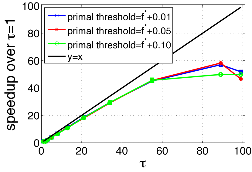
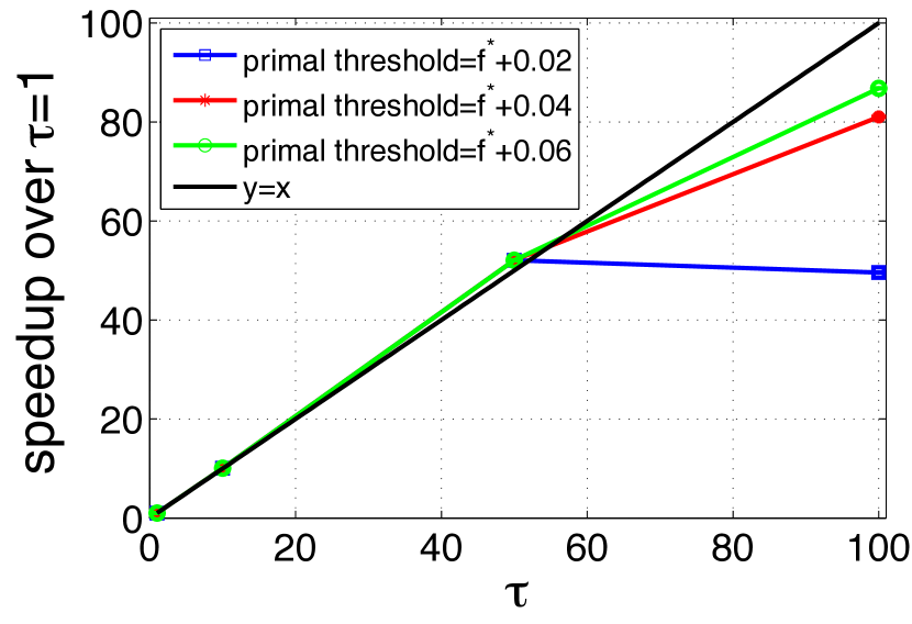
We conduct simulations to study the effect of mini-batch size τ𝜏\tau, where larger τ𝜏\tau implies greater degrees of parallelism as each worker can solve one or more subproblems in a mini-batch. In our simulation for structural SVM we use sequence labeling task on a subset of the OCR dataset [37] (n=6251,d=4082)formulae-sequence𝑛6251𝑑4082(n=6251,d=4082). The subproblem can be solved using the Viterbi algorithm. The speedup on this dataset is shown in Figure 1(a). For this dataset, we use λ=1𝜆1\lambda=1 with weighted averaging and line-search throughout. We measure the speedup for a particular τ>1𝜏1\tau>1 in terms of the number of epochs (Algorithm 1) required to converge relative to τ=1𝜏1\tau=1, which corresponds to Bcfw. Figure 1(a) shows that Ap-Bcfw achieves linear speedup for mini-batch size up to τ50𝜏50\tau\approx 50. Further speedup is sensitive to the convergence criteria, where more stringent thresholds lead to lower speed-ups. This is because large mini-batch sizes introduce errors, which reduces progress per update, and is consistent with existing work on the effect of parameter staleness on convergence [19, 10]. This suggests that it might be possible to use more workers initially for a large speedup and reduce parallelism as the algorithm approaches the optimum.

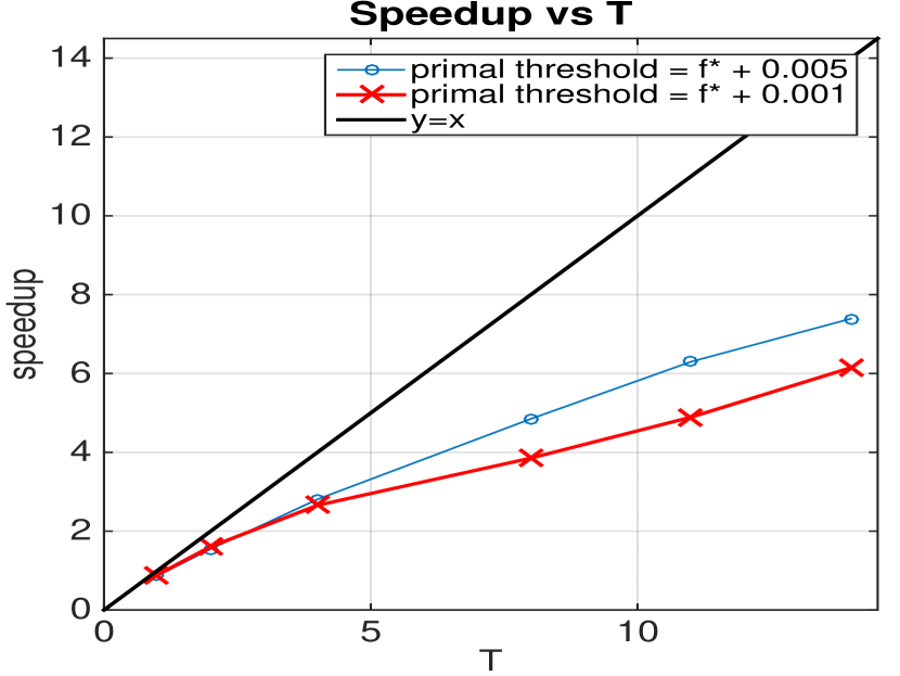
In our simulation for Group Fused Lasso, we generate a piecewise constant dataset of size (n=100,d=10formulae-sequence𝑛100𝑑10n=100,d=10, in Eq. 2) with Gaussian noise. We use λ=0.01𝜆0.01\lambda=0.01 and a primal suboptimality threshold as our convergence criterion. At each iteration, we solve τ𝜏\tau subproblems (i.e. the mini-batch size). Figure 1(b) shows the speed-up over τ=1𝜏1\tau=1 (Bcfw). Similar to the structural SVM, the speedup is almost perfect for small τ𝜏\tau (τ55𝜏55\tau\leq 55) but tapers off for large τ𝜏\tau to varying degrees depending on the convergence thresholds.
Refer to caption
(a) Structural SVM on OCR dataset (n=6251)
Refer to caption
(b) Group Fused Lasso (n=100)
Figure 1: Performance improvement with τ𝜏\tau for (a) Structual SVM on the OCR dataset [37] and (b) Group Fused Lasso on a synthetic dataset. fsuperscript𝑓f^{*} denotes primal optimum.

3.2 Shared Memory Parallel Workers

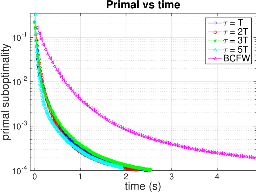
We implement Ap-Bcfw for the structural SVM in a multicore shared-memory system using the full OCR dataset (n=6877)𝑛6877(n=6877). All shared-memory experiments were implemented in C++ and conducted on a 16-core machine with Intel(R) Xeon(R) CPU E5-2450 2.10GHz processors and 128G RAM. We first fix the number of workers at T=8𝑇8T=8 and vary the mini-batch size τ𝜏\tau. Figure 2(a) shows the absolute convergence (i.e. the convergence per second). We note that Ap-Bcfw outperforms single-threaded Bcfw under all investigated τ𝜏\tau, showing the efficacy of parallelization. Within Ap-Bcfw, convergence improves with increasing mini-batch sizes up to τ=3T𝜏3𝑇\tau=3T, but worsens when τ=5T𝜏5𝑇\tau=5T as the error from the large mini-batch size dominates additional computation. The optimal τ𝜏\tau for a given number of workers (T𝑇T) depends on both the dataset (how “coupled” are the coordinates) and also system implementations (how costly is the synchronization as the system scales).

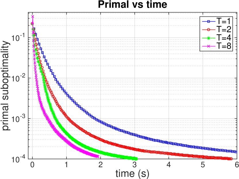
Since speedup for a given T𝑇T depends on τ𝜏\tau, we search for the optimal τ𝜏\tau across multiples of T𝑇T to find the best speedup for each T𝑇T. Figure 2(b) shows faster convergence of Ap-Bcfw over Bcfw (T=1𝑇1T=1) when T>1𝑇1T>1 workers are available. It is important to note that the x-axis is wall-clock time rather than the number of epochs.

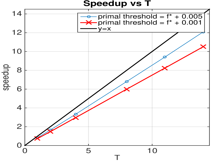
Figure 2(c) shows the speedup with varying T𝑇T. Ap-Bcfw achieves near-linear speed up for smaller T𝑇T. The speed-up curve tapers off for larger T𝑇T for two reasons: (1) Large T𝑇T incurs higher system overheads, and thus needs larger τ𝜏\tau to utilize CPU efficiently; (2) Larger τ𝜏\tau incurs errors as shown in Fig. 1(a). If the subproblems were more time-consuming to solve, the affect of system overhead would be reduced. We simulate harder subproblems by simply solving them msimilar-to𝑚absentm\simUniform(5,15)515(5,15) times instead of just once. The speedup is nearly perfect as shown in Figure 2(d). Again, we observe that a more generous convergence threshold produces higher speedup, suggesting that resource scheduling could be useful (e.g., allocate more CPUs initially and fewer as algorithm converges).
Refer to caption
(a)
Refer to caption
(b)
Refer to caption
(c)
Refer to caption
(d)
Figure 2: From left: (a) Primal suboptimality vs wall-clock time using 8 workers (T=8𝑇8T=8) and various mini-batch sizes τ𝜏\tau. (b) Primal suboptimality vs wall-clock time for varying T𝑇T with best τ𝜏\tau chosen for each T𝑇T separately. (c) Speedup via parallelization with the best τ𝜏\tau chosen among multiples of T𝑇T (T,2T,𝑇2𝑇T,2T,...) for each T𝑇T. (d) The same with longer subproblems.

3.3 Performance gain with asynchronous updates

We compare Ap-Bcfw with a synchronous version of the algorithm (Sp-Bcfw) where the server assigns τ/T𝜏𝑇\tau/T subproblems to each worker, then waits for and accumulates the solutions before proceeding to the next iteration. We simulate workers of varying slow-downs in our shared-memory setup by assigning a return probability pi(0,1]subscript𝑝𝑖01p_{i}\in(0,1] to each worker wisubscript𝑤𝑖w_{i}. After solving each subproblem, worker wisubscript𝑤𝑖w_{i} reports the solution to the server with probability pisubscript𝑝𝑖p_{i}. Thus a worker with pi=0.8subscript𝑝𝑖0.8p_{i}=0.8 will drop 20% of the updates on average corresponding to 20%percent2020\% slow-down.

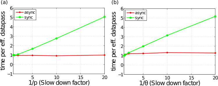
We use T=14𝑇14T=14 workers for the experiments in this section. We first simulate the scenario with just one straggler with return probability p(0,1]𝑝01p\in(0,1] while the other workers run at full speed (p=1)𝑝1(p=1). Figure 3(a) shows that the average time per effective datapass (over 20 passes and 5 runs) of Ap-Bcfw stays almost unchanged with slowdown factor 1/p1𝑝1/p of the straggler, whereas it increases linearly for Sp-Bcfw. This is because Ap-Bcfw relies on the average available worker processing power, while Sp-Bcfw is only as fast as the slowest worker.

Next, we simulate a heterogeneous environment where the workers have varying speeds. While varying a parameter θ[0,1]𝜃01\theta\in[0,1], we set pi=θ+i/Tsubscript𝑝𝑖𝜃𝑖𝑇p_{i}=\theta+i/T for i=1,,T𝑖1𝑇i=1,\cdots,T. Figure 3(b) shows that Ap-Bcfw slows down by only a factor of 1.4 compared to the no-straggler case. Assuming that the server and worker each takes about half the (wall-clock) time on average per epoch, we would expect the run time to increase by 50% if average worker speed halves, which is the case if θ=0𝜃0\theta=0 (i.e., 1θ1𝜃\frac{1}{\theta}\rightarrow\infty). Therefore a factor of 1.4 is reasonable. The performance of Sp-Bcfw is almost identical to that in the previous experiment as its speed is determined by the slowest worker. Thus our experiments show that Ap-Bcfw is robust to stragglers and system heterogeneity.
Refer to caption
Figure 3: Average time per effective data pass in asynchronous and synchronous modes for two cases: one worker is slow with return probability p𝑝p (left); workers have return probabilities (pi(p_{i}s))) uniformly in [θ,1]𝜃1[\theta,1] (right). Times normalized separately for Ap-Bcfw, Sp-Bcfw w.r.t. to the setup where workers run at full speed.

3.4 Convergence under unbounded heavy-tailed delay

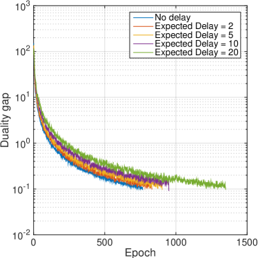
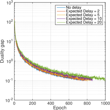
In this section, we illustrate the mild effect of delay on convergence by randomly drawing an independent delay variable for each worker. For simplicity, we use τ=1𝜏1\tau=1 (Bcfw) on the same group fused lasso problem as in Section 3.1. We sample ϰitalic-ϰ\varkappa using either a Poisson distribution or a heavy-tailed Pareto distribution (round to the nearest integer). The Pareto distribution is chosen with shape parameter α=2𝛼2\alpha=2 and scale parameter xm=κ/2subscript𝑥𝑚𝜅2x_{m}=\kappa/2 such that 𝔼ϰ=κ𝔼italic-ϰ𝜅\mathbb{E}\varkappa=\kappa and Varϰ=Varitalic-ϰ\mathrm{Var}\varkappa=\infty. During the experiment, at iteration k𝑘k, any updates that were based on a delay greater than k/2𝑘2k/2 are dropped (as our theory demanded). The results are shown in Figure 4. Observe that for both cases, the impact of the delay is rather mild. With expected delay up to 202020, the algorithm only takes fewer than twice as many iterations to converge.
Refer to caption
Refer to caption
Figure 4: Illustrations of the convergence Bcfw with delayed updates. On the left, we have the delay sampled from a Poisson distribution. The figure on the right is for delay sampled from a Pareto distribution. We run each problem until the duality gap reaches 0.10.10.1.

4 Conclusion

In this paper, we propose an asynchronous parallel generalization of the block-coordinate Frank-Wolfe method [24] and provide intuitive conditions under which it has a provable speed-up over Bcfw. The asynchronous updates allow our method to be robust to stragglers and node failure as the speed of Ap-Bcfw depends on average worker speed instead of the slowest. We demonstrate the effectiveness of the algorithm in structural SVM and Group Fused Lasso with both controlled simulation and real-data experiments on a multi-core workstation. For the structural SVM, it leads to a speed-up over the state-of-the-art Bcfw by an order of magnitude using 16 parallel processors. As a projection-free Frank-Wolfe method, we expect our algorithm to be very competitive in large-scale constrained optimization problems, especially when projections are expensive. Future work includes analysis for the strongly convex case and ultimately releasing a carefully implemented software package for practitioners to deploy in Big Data applications.

References

  • Alaíz et al. [2013] Alaíz, Carlos M, Barbero, Álvaro, and Dorronsoro, José R. Group fused lasso. In Artificial Neural Networks and Machine Learning–ICANN 2013, pp.  66–73. Springer, 2013.
  • Bach [2013] Bach, Francis. Conditional gradients everywhere. 2013.
  • Beck & Tetruashvili [2013] Beck, Amir and Tetruashvili, Luba. On the convergence of block coordinate descent type methods. SIAM Journal on Optimization, 23(4):2037–2060, 2013.
  • Bellet et al. [2014] Bellet, Aurélien, Liang, Yingyu, Garakani, Alireza Bagheri, Balcan, Maria-Florina, and Sha, Fei. Distributed frank-wolfe algorithm: A unified framework for communication-efficient sparse learning. CoRR, abs/1404.2644, 2014.
  • Bleakley & Vert [2011] Bleakley, Kevin and Vert, Jean-Philippe. The group fused lasso for multiple change-point detection. arXiv, 2011.
  • Bredies et al. [2009] Bredies, Kristian, Lorenz, Dirk A, and Maass, Peter. A generalized conditional gradient method and its connection to an iterative shrinkage method. Computational Optimization and Applications, 42(2):173–193, 2009.
  • Clarkson [2010] Clarkson, Kenneth L. Coresets, sparse greedy approximation, and the Frank-Wolfe algorithm. ACM Transactions on Algorithms (TALG), 6(4):63, 2010.
  • Collins et al. [2008] Collins, Michael, Globerson, Amir, Koo, Terry, Carreras, Xavier, and Bartlett, Peter L. Exponentiated gradient algorithms for conditional random fields and max-margin markov networks. JMLR, 9:1775–1822, 2008.
  • Dai et al. [2013] Dai, Wei, Wei, Jinliang, Zheng, Xun, Kim, Jin Kyu, Lee, Seunghak, Yin, Junming, Ho, Qirong, and Xing, Eric P. Petuum: A framework for iterative-convergent distributed ml. arXiv:1312.7651, 2013.
  • Dai et al. [2014] Dai, Wei, Kumar, Abhimanu, Wei, Jinliang, Ho, Qirong, Gibson, Garth, and Xing, Eric P. High-performance distributed ml at scale through parameterserver consistency models. In AAAI, 2014.
  • Fercoq & Richtárik [2015] Fercoq, Olivier and Richtárik, Peter. Accelerated, parallel, and proximal coordinate descent. SIAM Journal on Optimization, 25(4):1997–2023, 2015.
  • Foygel et al. [2012] Foygel, Rina, Horrell, Michael, Drton, Mathias, and Lafferty, John D. Nonparametric reduced rank regression. In NIPS’12, pp.  1628–1636, 2012.
  • Frank & Wolfe [1956] Frank, Marguerite and Wolfe, Philip. An algorithm for quadratic programming. Naval research logistics quarterly, 3(1-2):95–110, 1956.
  • Freund & Grigas [2014] Freund, Robert M. and Grigas, Paul. New analysis and results for the frank–wolfe method. Mathematical Programming, 155(1):199–230, 2014. ISSN 1436-4646.
  • Fujishige & Isotani [2011] Fujishige, Satoru and Isotani, Shigueo. A submodular function minimization algorithm based on the minimum-norm base. Pacific Journal of Optimization, 7(1):3–17, 2011.
  • Garber & Hazan [2013] Garber, Dan and Hazan, Elad. A linearly convergent conditional gradient algorithm with applications to online and stochastic optimization. arXiv:1301.4666, 2013.
  • Harchaoui et al. [2015] Harchaoui, Zaid, Juditsky, Anatoli, and Nemirovski, Arkadi. Conditional gradient algorithms for norm-regularized smooth convex optimization. Mathematical Programming, 152(1-2):75–112, 2015. ISSN 0025-5610.
  • Hazan & Kale [2012] Hazan, Elad and Kale, Satyen. Projection-free online learning. In ICML’12, 2012.
  • Ho et al. [2013] Ho, Qirong, Cipar, James, Cui, Henggang, Lee, Seunghak, Kim, Jin Kyu, Gibbons, Phillip B., Gibson, Garth A., Ganger, Greg, and Xing, Eric. More effective distributed ml via a stale synchronous parallel parameter server. In NIPS’13. 2013.
  • Jaggi [2011] Jaggi, Martin. Sparse convex optimization methods for machine learning. PhD thesis, Diss., Eidgenössische Technische Hochschule ETH Zürich, Nr. 20013, 2011, 2011.
  • Jaggi [2013] Jaggi, Martin. Revisiting Frank-Wolfe: Projection-free sparse convex optimization. In ICML’13, pp.  427–435, 2013.
  • Jegelka et al. [2013] Jegelka, Stefanie, Bach, Francis, and Sra, Suvrit. Reflection methods for user-friendly submodular optimization. In NIPS’13, pp.  1313–1321, 2013.
  • Lacoste-Julien & Jaggi [2015] Lacoste-Julien, Simon and Jaggi, Martin. On the global linear convergence of frank-wolfe optimization variants. In NIPS’15, pp.  496–504, 2015.
  • Lacoste-Julien et al. [2013] Lacoste-Julien, Simon, Jaggi, Martin, Schmidt, Mark, and Pletscher, Patrick. Block-coordinate frank-wolfe optimization for structural svms. In ICML’13, pp.  53–61, 2013.
  • Lafond et al. [2015] Lafond, Jean, Wai, Hoi-To, and Moulines, Eric. Convergence analysis of a stochastic projection-free algorithm. arXiv:1510.01171, 2015.
  • LeBlanc et al. [1975] LeBlanc, Larry J, Morlok, Edward K, and Pierskalla, William P. An efficient approach to solving the road network equilibrium traffic assignment problem. Transportation Research, 9(5):309–318, 1975.
  • Lee et al. [2014] Lee, Seunghak, Kim, Jin Kyu, Zheng, Xun, Ho, Qirong, Gibson, Garth A, and Xing, Eric P. On model parallelization and scheduling strategies for distributed machine learning. In NIPS’14, pp.  2834–2842, 2014.
  • Li et al. [2013] Li, Mu, Zhou, Li, Yang, Zichao, Li, Aaron, Xia, Fei, Andersen, David G, and Smola, Alexander. Parameter server for distributed machine learning. In NIPS Workshop: Big Learning, 2013.
  • Liu et al. [2013] Liu, Ji, Musialski, Przemyslaw, Wonka, Peter, and Ye, Jieping. Tensor completion for estimating missing values in visual data. Pattern Analysis and Machine Intelligence, IEEE Transactions on, 35(1):208–220, 2013.
  • Liu et al. [2014] Liu, Ji, Wright, Stephen J, Ré, Christopher, and Bittorf, Victor. An asynchronous parallel stochastic coordinate descent algorithm. JMLR, 2014.
  • Mitzenmacher [2001] Mitzenmacher, Michael. The power of two choices in randomized load balancing. Parallel and Distributed Systems, IEEE Transactions on, 12(10):1094–1104, 2001.
  • Nesterov [2012] Nesterov, Yu. Efficiency of coordinate descent methods on huge-scale optimization problems. SIAM Journal on Optimization, 22(2):341–362, 2012.
  • Niu et al. [2011] Niu, Feng, Recht, Benjamin, Ré, Christopher, and Wright, Stephen J. Hogwild!: A lock-free approach to parallelizing stochastic gradient descent. arXiv:1106.5730, 2011.
  • Ouyang & Gray [2010] Ouyang, Hua and Gray, Alexander G. Fast stochastic Frank-Wolfe algorithms for nonlinear SVMs. In SDM, 2010.
  • Raab & Steger [1998] Raab, Martin and Steger, Angelika. Balls into bins - a simple and tight analysis. In Randomization and Approximation Techniques in Computer Science, pp.  159–170. Springer, 1998.
  • Richtárik & Takáč [2012] Richtárik, Peter and Takáč, Martin. Parallel coordinate descent methods for big data optimization. arXiv:1212.0873, 2012.
  • Taskar et al. [2004] Taskar, Ben, Guestrin, Carlos, and Koller, Daphne. Max-margin Markov networks. In NIPS’04, pp.  25–32. MIT Press, 2004.
  • Tsitsiklis et al. [1986] Tsitsiklis, John N, Bertsekas, Dimitri P, Athans, Michael, et al. Distributed asynchronous deterministic and stochastic gradient optimization algorithms. IEEE transactions on automatic control, 31(9), 1986.
  • Yu & Joachims [2009] Yu, Chun-Nam John and Joachims, Thorsten. Learning structural svms with latent variables. In ICML’09, pp.  1169–1176. ACM, 2009.
  • Zhang et al. [2012] Zhang, Xinhua, Yu, Yaoliang, and Schuurmans, Dale. Accelerated training for matrix-norm regularization: A boosting approach. In NIPS’12, pp.  2915–2923, 2012.
  • Zhang et al. [2013] Zhang, Xinhua, Yu, Yao-Liang, and Schuurmans, Dale. Polar operators for structured sparse estimation. In NIPS’13, pp.  82–90, 2013.

Appendix A Convergence analysis

We provide a self-contained convergence proof in this section. The skeleton of our convergence proof follow closely from Lacoste-Julien et al. [24] and Jaggi [21]. There are a few subtle modification and improvements that we need to add due to our weaker definition of approximate oracle call that is nearly correct only in expectation. The delayed convergence is new and interesting for the best of our knowledge, which uses a simple result in “load balancing” [31].

Note that for the cleanness of the presentation, we focus on the primal and primal-dual convergence of the version of the algorithms with pre-defined step sizes and additive approximate subroutine, it is simple to extend the same analysis for line-search variant and multiplicative approximation.

A.1 Primal Convergence

Lemma 2.

Denote the gap between current f(x(k))𝑓superscript𝑥𝑘f(x^{(k)}) and the optimal f(x)𝑓superscript𝑥f(x^{*}) to be h(x(k))superscript𝑥𝑘h(x^{(k)}). The iterative updates in Algorithm 1(with arbitrary fixed stepsize λ𝜆\lambda or by the coordinate-line search) obey

𝔼h(x(k+1))(1γτn)𝔼h(x(k))+γ2(1+δ)2Cfτ.𝔼superscript𝑥𝑘11𝛾𝜏𝑛𝔼superscript𝑥𝑘superscript𝛾21𝛿2superscriptsubscript𝐶𝑓𝜏\mathbb{E}h(x^{(k+1)})\leq(1-\frac{\gamma\tau}{n})\mathbb{E}h(x^{(k)})+\frac{\gamma^{2}(1+\delta)}{2}C_{f}^{\tau}.

where the expectation is taken over the joint randomness all the way to iteration k+1𝑘1k+1.

Proof.

Let x:=x(k)assign𝑥superscript𝑥𝑘x:=x^{(k)} for notational convenience. We prove the result for Algorithm  1 first. Apply the definition of Cf(S)superscriptsubscript𝐶𝑓𝑆C_{f}^{(S)} and then apply the definition of the additive approximation in (6), to get

f(xlinesearch(k+1))𝑓subscriptsuperscript𝑥𝑘1linesearch\displaystyle f(x^{(k+1)}_{\mathrm{line-search}}) f(xγ(k+1))=f(x+γiS(s[i]x[i]))absent𝑓subscriptsuperscript𝑥𝑘1𝛾𝑓𝑥𝛾subscript𝑖𝑆subscript𝑠delimited-[]𝑖subscript𝑥delimited-[]𝑖\displaystyle\leq f(x^{(k+1)}_{\gamma})=f(x+\gamma\sum_{i\in S}(s_{[i]}-x_{[i]}))
f(x)+γiSs[i]x[i],[i]f(x)+γ22Cf(S)absent𝑓𝑥𝛾subscript𝑖𝑆subscript𝑠delimited-[]𝑖subscript𝑥delimited-[]𝑖subscriptdelimited-[]𝑖𝑓𝑥superscript𝛾22superscriptsubscript𝐶𝑓𝑆\displaystyle\leq f(x)+\gamma\sum_{i\in S}\langle s_{[i]}-x_{[i]},\nabla_{[i]}f(x)\rangle+\frac{\gamma^{2}}{2}C_{f}^{(S)}
=f(x)+γs[S]x[S],[S]f(x)+γ22Cf(S)absent𝑓𝑥𝛾subscript𝑠delimited-[]𝑆subscript𝑥delimited-[]𝑆subscriptdelimited-[]𝑆𝑓𝑥superscript𝛾22superscriptsubscript𝐶𝑓𝑆\displaystyle=f(x)+\gamma\langle s_{[S]}-x_{[S]},\nabla_{[S]}f(x)\rangle+\frac{\gamma^{2}}{2}C_{f}^{(S)}

Subtract f(x)𝑓superscript𝑥f(x^{*}) on both sides we get:

h(x(k+1))h(x(k))+γs[S]x[S](k),[S]f(x(k))+γ22Cf(S)superscript𝑥𝑘1superscript𝑥𝑘𝛾subscript𝑠delimited-[]𝑆subscriptsuperscript𝑥𝑘delimited-[]𝑆subscriptdelimited-[]𝑆𝑓superscript𝑥𝑘superscript𝛾22superscriptsubscript𝐶𝑓𝑆\displaystyle h(x^{(k+1)})\leq h(x^{(k)})+\gamma\langle s_{[S]}-x^{(k)}_{[S]},\nabla_{[S]}f(x^{(k)})\rangle+\frac{\gamma^{2}}{2}C_{f}^{(S)}

Now take the expectation over the entire history then apply (6) and definition of the surrogate duality gap (7), we obtain

𝔼h(x(k+1))𝔼superscript𝑥𝑘1absent\displaystyle\mathbb{E}h(x^{(k+1)})\leq 𝔼h(x(k))+𝔼{γs[S]x[S](k),[S]f(x(k))}+𝔼γ22Cf(S)𝔼superscript𝑥𝑘𝔼𝛾subscript𝑠delimited-[]𝑆subscriptsuperscript𝑥𝑘delimited-[]𝑆subscriptdelimited-[]𝑆𝑓superscript𝑥𝑘𝔼superscript𝛾22superscriptsubscript𝐶𝑓𝑆\displaystyle\mathbb{E}h(x^{(k)})+\mathbb{E}\left\{\gamma\langle s_{[S]}-x^{(k)}_{[S]},\nabla_{[S]}f(x^{(k)})\rangle\right\}+\mathbb{E}\frac{\gamma^{2}}{2}C_{f}^{(S)}
=\displaystyle= 𝔼h(x(k))+γ𝔼{s[S],[S]f(x(k))mins(S)s,[S]f(x(k))}𝔼superscript𝑥𝑘𝛾𝔼subscript𝑠delimited-[]𝑆subscriptdelimited-[]𝑆𝑓superscript𝑥𝑘subscript𝑠superscript𝑆𝑠subscriptdelimited-[]𝑆𝑓superscript𝑥𝑘\displaystyle\mathbb{E}h(x^{(k)})+\gamma\mathbb{E}\left\{\langle s_{[S]},\nabla_{[S]}f(x^{(k)})\rangle-\min_{s\in\mathcal{M}^{(S)}}\langle s,\nabla_{[S]}f(x^{(k)})\rangle\right\}
γ𝔼{x[S](k),[S]f(x(k))mins(S)s,[S]f(x(k))}+γ22Cfτ\displaystyle-\gamma\mathbb{E}\left\{\langle x^{(k)}_{[S]},\nabla_{[S]}f(x^{(k)})\rangle-\min_{s\in\mathcal{M}^{(S)}}\langle s,\nabla_{[S]}f(x^{(k)})\right\}+\frac{\gamma^{2}}{2}C_{f}^{\tau}
\displaystyle\leq 𝔼h(x(k))+γ2δ2Cfτγ𝔼xk𝔼S|xkiSg(i)(x(k))+γ22Cfτ𝔼superscript𝑥𝑘superscript𝛾2𝛿2superscriptsubscript𝐶𝑓𝜏𝛾subscript𝔼superscript𝑥𝑘subscript𝔼conditional𝑆superscript𝑥𝑘subscript𝑖𝑆superscript𝑔𝑖superscript𝑥𝑘superscript𝛾22superscriptsubscript𝐶𝑓𝜏\displaystyle\mathbb{E}h(x^{(k)})+\frac{\gamma^{2}\delta}{2}C_{f}^{\tau}-\gamma\mathbb{E}_{x^{k}}\mathbb{E}_{S|x^{k}}\sum_{i\in S}g^{(i)}(x^{(k)})+\frac{\gamma^{2}}{2}C_{f}^{\tau}
=\displaystyle= 𝔼h(x(k))+γ2δ2Cfτγ𝔼xkτng(x(k))+γ22Cfτ𝔼superscript𝑥𝑘superscript𝛾2𝛿2superscriptsubscript𝐶𝑓𝜏𝛾subscript𝔼superscript𝑥𝑘𝜏𝑛𝑔superscript𝑥𝑘superscript𝛾22superscriptsubscript𝐶𝑓𝜏\displaystyle\mathbb{E}h(x^{(k)})+\frac{\gamma^{2}\delta}{2}C_{f}^{\tau}-\gamma\mathbb{E}_{x^{k}}\frac{\tau}{n}g(x^{(k)})+\frac{\gamma^{2}}{2}C_{f}^{\tau} (13)
\displaystyle\leq (1γτn)𝔼h(x(k))+γ2(1+δ)2Cfτ.1𝛾𝜏𝑛𝔼superscript𝑥𝑘superscript𝛾21𝛿2superscriptsubscript𝐶𝑓𝜏\displaystyle(1-\frac{\gamma\tau}{n})\mathbb{E}h(x^{(k)})+\frac{\gamma^{2}(1+\delta)}{2}C_{f}^{\tau}.

The last inequality follows from the property of the surrogate duality gap g(x(k))h(x(k))𝑔superscript𝑥𝑘superscript𝑥𝑘g(x^{(k)})\geq h(x^{(k)}) due to the fact that g(x)=f(x)f()𝑔𝑥𝑓𝑥superscript𝑓g(x)=f(x)-f^{*}(\cdot). This completes the proof of the descent lemma. ∎

Now we are ready to state the proof for Theorem 1.

Proof of Theorem 1.

We follow the proof in Theorem C.1 in Lacoste-Julien et al. [24] to prove the statement for Algorithm 1. The difference is that we use a different and carefully chosen sequence of step size.

Take C=h0+n(1+δ)Cfτ,𝐶subscript0𝑛1𝛿subscriptsuperscript𝐶𝜏𝑓C=h_{0}+n(1+\delta)C^{\tau}_{f}, and denote 𝔼h(x(k))𝔼superscript𝑥𝑘\mathbb{E}h(x^{(k)}) as hksubscript𝑘h_{k} for short hands. The inequality in Lemma 2 simplifies to

hk+1(1γτn)hk+γ22nC.subscript𝑘11𝛾𝜏𝑛subscript𝑘superscript𝛾22𝑛𝐶h_{k+1}\leq\left(1-\frac{\gamma\tau}{n}\right)h_{k}+\frac{\gamma^{2}}{2n}C.

Now we will prove hk2nCτ2k+2nsubscript𝑘2𝑛𝐶superscript𝜏2𝑘2𝑛h_{k}\leq\frac{2nC}{\tau^{2}k+2n} for γk=2nττ2k+2nsubscript𝛾𝑘2𝑛𝜏superscript𝜏2𝑘2𝑛\gamma_{k}=\frac{2n\tau}{\tau^{2}k+2n} by induction. The base case k=0𝑘0k=0 is trivially true since C>h0𝐶subscript0C>h_{0}. Assuming that the claim holds for k𝑘k, we apply the induction hypothesis and the above inequality is reduced to

hk+1subscript𝑘1\displaystyle h_{k+1} (1γτn)hk+γ22nC2nCτ2k+2n[1γτn+τ2k+2n2nγ22n]absent1𝛾𝜏𝑛subscript𝑘superscript𝛾22𝑛𝐶2𝑛𝐶superscript𝜏2𝑘2𝑛delimited-[]1𝛾𝜏𝑛superscript𝜏2𝑘2𝑛2𝑛superscript𝛾22𝑛\displaystyle\leq(1-\frac{\gamma\tau}{n})h_{k}+\frac{\gamma^{2}}{2n}C\leq\frac{2nC}{\tau^{2}k+2n}\left[1-\frac{\gamma\tau}{n}+\frac{\tau^{2}k+2n}{2n}\frac{\gamma^{2}}{2n}\right]
=2nCτ2k+2n[τ2k+2nτ2k+2n2nττ2k+2nτn+(2nτ)24n2(τ2k+2n)]absent2𝑛𝐶superscript𝜏2𝑘2𝑛delimited-[]superscript𝜏2𝑘2𝑛superscript𝜏2𝑘2𝑛2𝑛𝜏superscript𝜏2𝑘2𝑛𝜏𝑛superscript2𝑛𝜏24superscript𝑛2superscript𝜏2𝑘2𝑛\displaystyle=\frac{2nC}{\tau^{2}k+2n}\left[\frac{\tau^{2}k+2n}{\tau^{2}k+2n}-\frac{2n\tau}{\tau^{2}k+2n}\cdot\frac{\tau}{n}+\frac{(2n\tau)^{2}}{4n^{2}(\tau^{2}k+2n)}\right]
=2nCτ2k+2nτ2k+2nτ2τ2k+2n2nCτ2k+2nτ2k+2nτ2+τ2τ2k+2n+τ2absent2𝑛𝐶superscript𝜏2𝑘2𝑛superscript𝜏2𝑘2𝑛superscript𝜏2superscript𝜏2𝑘2𝑛2𝑛𝐶superscript𝜏2𝑘2𝑛superscript𝜏2𝑘2𝑛superscript𝜏2superscript𝜏2superscript𝜏2𝑘2𝑛superscript𝜏2\displaystyle=\frac{2nC}{\tau^{2}k+2n}\cdot\frac{\tau^{2}k+2n-\tau^{2}}{\tau^{2}k+2n}\leq\frac{2nC}{\tau^{2}k+2n}\cdot\frac{\tau^{2}k+2n-\tau^{2}+\tau^{2}}{\tau^{2}k+2n+\tau^{2}}
=2nCτ2(k+1)+2n.absent2𝑛𝐶superscript𝜏2𝑘12𝑛\displaystyle=\frac{2nC}{\tau^{2}(k+1)+2n}.

This completes the induction and hence the proof for the primal convergence for Algorithm 1. ∎

A.2 Convergence of the surrogate duality gap

Proof of Theorem 2.

We mimic the proof in Lacoste-Julien et al. [24, Section C.3] for the analogous result closely, and we will use the same notation for hksubscript𝑘h_{k}and C𝐶C as in the proof for primal convergence, moreover denote gk=𝔼g(x(k))subscript𝑔𝑘𝔼𝑔superscript𝑥𝑘g_{k}=\mathbb{E}g(x^{(k)}) First from (13) in the proof of Lemma 2, we have

hk+1hkγτngk+γ22nC.subscript𝑘1subscript𝑘𝛾𝜏𝑛subscript𝑔𝑘superscript𝛾22𝑛𝐶h_{k+1}\leq h_{k}-\frac{\gamma\tau}{n}g_{k}+\frac{\gamma^{2}}{2n}C.

Rearrange the terms, we get

gknγτ(hkhk+1)+γC2τ.subscript𝑔𝑘𝑛𝛾𝜏subscript𝑘subscript𝑘1𝛾𝐶2𝜏g_{k}\leq\frac{n}{\gamma\tau}(h_{k}-h_{k+1})+\frac{\gamma C}{2\tau}. (14)

The idea is that if we take an arbitrary convex combination of {g1,,gK}subscript𝑔1subscript𝑔𝐾\{g_{1},...,g_{K}\}, the result will be within the convex hull, namely between the minimum and the maximum, hence proven the existence claim in the theorem. By choosing weight ρk:=k/SKassignsubscript𝜌𝑘𝑘subscript𝑆𝐾\rho_{k}:=k/S_{K} where normalization constant SK=K(K+1)2subscript𝑆𝐾𝐾𝐾12S_{K}=\frac{K(K+1)}{2} and taking the convex combination of both side of (14), we have

𝔼(mink[K]gk)𝔼subscript𝑘delimited-[]𝐾subscript𝑔𝑘\displaystyle\mathbb{E}(\min_{k\in[K]}g_{k}) k=0Kρkgknτk=1Kρk(hkγkhk+1γk)+k=0KρkγkC2τabsentsuperscriptsubscript𝑘0𝐾subscript𝜌𝑘subscript𝑔𝑘𝑛𝜏superscriptsubscript𝑘1𝐾subscript𝜌𝑘subscript𝑘subscript𝛾𝑘subscript𝑘1subscript𝛾𝑘superscriptsubscript𝑘0𝐾subscript𝜌𝑘subscript𝛾𝑘𝐶2𝜏\displaystyle\leq\sum_{k=0}^{K}\rho_{k}g_{k}\leq\frac{n}{\tau}\sum_{k=1}^{K}\rho_{k}(\frac{h_{k}}{\gamma_{k}}-\frac{h_{k+1}}{\gamma_{k}})+\sum_{k=0}^{K}\rho_{k}\gamma_{k}\frac{C}{2\tau}
=nτ(h0ρ0γ0hK+1ρkγk)+nτk=0K1hk+1(ρk+1γk+1ρkγk)+k=0KρkγkC2τabsent𝑛𝜏subscript0subscript𝜌0subscript𝛾0subscript𝐾1subscript𝜌𝑘subscript𝛾𝑘𝑛𝜏superscriptsubscript𝑘0𝐾1subscript𝑘1subscript𝜌𝑘1subscript𝛾𝑘1subscript𝜌𝑘subscript𝛾𝑘superscriptsubscript𝑘0𝐾subscript𝜌𝑘subscript𝛾𝑘𝐶2𝜏\displaystyle=\frac{n}{\tau}(\frac{h_{0}\rho_{0}}{\gamma_{0}}-h_{K+1}\frac{\rho_{k}}{\gamma_{k}})+\frac{n}{\tau}\sum_{k=0}^{K-1}h_{k+1}(\frac{\rho_{k+1}}{\gamma_{k+1}}-\frac{\rho_{k}}{\gamma_{k}})+\sum_{k=0}^{K}\rho_{k}\gamma_{k}\frac{C}{2\tau}
nτk=0K1hk+1(ρk+1γk+1ρkγk)+k=0KρkγkC2τabsent𝑛𝜏superscriptsubscript𝑘0𝐾1subscript𝑘1subscript𝜌𝑘1subscript𝛾𝑘1subscript𝜌𝑘subscript𝛾𝑘superscriptsubscript𝑘0𝐾subscript𝜌𝑘subscript𝛾𝑘𝐶2𝜏\displaystyle\leq\frac{n}{\tau}\sum_{k=0}^{K-1}h_{k+1}(\frac{\rho_{k+1}}{\gamma_{k+1}}-\frac{\rho_{k}}{\gamma_{k}})+\sum_{k=0}^{K}\rho_{k}\gamma_{k}\frac{C}{2\tau} (15)

Note that ρ0=0subscript𝜌00\rho_{0}=0, so we simply dropped a negative term in last line. Applying the step size γk=2nτ/(τ2k+2n)subscript𝛾𝑘2𝑛𝜏superscript𝜏2𝑘2𝑛\gamma_{k}=2n\tau/(\tau^{2}k+2n), we get

ρk+1γk+1ρkγksubscript𝜌𝑘1subscript𝛾𝑘1subscript𝜌𝑘subscript𝛾𝑘\displaystyle\frac{\rho_{k+1}}{\gamma_{k+1}}-\frac{\rho_{k}}{\gamma_{k}} =k+1SKτ2(k+1)2n2nτkSKτ2k+2n2nτabsent𝑘1subscript𝑆𝐾superscript𝜏2𝑘12𝑛2𝑛𝜏𝑘subscript𝑆𝐾superscript𝜏2𝑘2𝑛2𝑛𝜏\displaystyle=\frac{k+1}{S_{K}}\frac{\tau^{2}(k+1)2n}{2n\tau}-\frac{k}{S_{K}}\frac{\tau^{2}k+2n}{2n\tau}
=12nSKτ[τ2(k+1)2+2n(k+1)τ2k22nk]absent12𝑛subscript𝑆𝐾𝜏delimited-[]superscript𝜏2superscript𝑘122𝑛𝑘1superscript𝜏2superscript𝑘22𝑛𝑘\displaystyle=\frac{1}{2nS_{K}\tau}\left[\tau^{2}(k+1)^{2}+2n(k+1)-\tau^{2}k^{2}-2nk\right]
=τ2(2k+1)+2n2nSKτ.absentsuperscript𝜏22𝑘12𝑛2𝑛subscript𝑆𝐾𝜏\displaystyle=\frac{\tau^{2}(2k+1)+2n}{2nS_{K}\tau}.

Plug the above back into (15) and use the bound hk+12nC/(τ2(k+1)+2n)subscript𝑘12𝑛𝐶superscript𝜏2𝑘12𝑛h_{k+1}\leq 2nC/(\tau^{2}(k+1)+2n), we get

𝔼(mink[K]gk)𝔼subscript𝑘delimited-[]𝐾subscript𝑔𝑘\displaystyle\mathbb{E}(\min_{k\in[K]}g_{k}) k=0KρkgknCτ2SKk=0K1τ2(2k+2)+2n2n2nτ(2k+1)+2n+k=0KkSK2nττ2k+2nC2τ\displaystyle\leq\sum_{k=0}^{K}\rho_{k}g_{k}\leq\frac{nC}{\tau^{2}S_{K}}\sum_{k=0}^{K-1}\frac{\tau^{2}(2k+2)+2n}{2n}\frac{2n}{\tau^{(}2k+1)+2n}+\sum_{k=0}^{K}\frac{k}{S_{K}}\frac{2n\tau}{\tau^{2}k+2n}\frac{C}{2\tau}
=nCτ2SK[k=0K1(1+τ2τ2(k+1)+2n)+k=1Kkτ2(τ2k+2n)]absent𝑛𝐶superscript𝜏2subscript𝑆𝐾delimited-[]superscriptsubscript𝑘0𝐾11superscript𝜏2superscript𝜏2𝑘12𝑛superscriptsubscript𝑘1𝐾𝑘superscript𝜏2superscript𝜏2𝑘2𝑛\displaystyle=\frac{nC}{\tau^{2}S_{K}}\left[\sum_{k=0}^{K-1}(1+\frac{\tau^{2}}{\tau^{2}(k+1)+2n})+\sum_{k=1}^{K}\frac{k\tau^{2}}{(\tau^{2}k+2n)}\right]
nCτ2SK[2K+K]=2nCτ2(K+1)3.absent𝑛𝐶superscript𝜏2subscript𝑆𝐾delimited-[]2𝐾𝐾2𝑛𝐶superscript𝜏2𝐾13\displaystyle\leq\frac{nC}{\tau^{2}S_{K}}\left[2K+K\right]=\frac{2nC}{\tau^{2}(K+1)}\cdot 3.

This completes the proof for K1𝐾1K\geq 1. ∎

Proof of Convergence with Delayed Gradient

The idea is that we are going to treat the updates calculated from the delayed gradients as an additive error and then invoke our convergence results that allow the oracle to be approximate. We will first present a lemma that we will use for the proof of Theorem 4.

Lemma 3.

Let x𝑥x\in\mathcal{M}, \|\cdot\| be a norm, Diam()D\mathrm{Diam}(\mathcal{M})_{\|\cdot\|}\leq D, L𝐿L be the gradient Lipschitz constant with respect to the given norm \|\cdot\|. Let κ𝜅\kappa be the maximum staleness of the gradient, γ𝛾\gamma be the largest stepsize in the past κ𝜅\kappa steps. Then

s~x,f(x)sx,f(x)+γκD2L~𝑠𝑥𝑓𝑥superscript𝑠𝑥𝑓𝑥𝛾𝜅superscript𝐷2𝐿\langle\tilde{s}-x,\nabla f(x)\rangle\leq\langle s^{*}-x,\nabla f(x)\rangle+\gamma\kappa D^{2}L
Proof.

Because s~~𝑠\tilde{s} minimizes s,f(x~)𝑠𝑓~𝑥\langle s,\nabla f(\tilde{x})\rangle over s𝑠s\in\mathcal{H}, we can write

ss~,f(x~)0.superscript𝑠~𝑠𝑓~𝑥0\langle s^{*}-\tilde{s},\nabla f(\tilde{x})\rangle\geq 0.

Using this and Hölder’s inequality, we can write

s~x,f(x)sx,f(x)s~s,f(x)f(x~)s~sf(x~)f(x)DLx~x.~𝑠𝑥𝑓𝑥superscript𝑠𝑥𝑓𝑥~𝑠superscript𝑠𝑓𝑥𝑓~𝑥norm~𝑠superscript𝑠subscriptnorm𝑓~𝑥𝑓𝑥𝐷𝐿norm~𝑥𝑥\langle\tilde{s}-x,\nabla f(x)\rangle-\langle s^{*}-x,\nabla f(x)\rangle\leq\langle\tilde{s}-s^{*},\nabla f(x)-\nabla f(\tilde{x})\rangle\leq\|\tilde{s}-s^{*}\|\|\nabla f(\tilde{x})-\nabla f(x)\|_{*}\leq DL\|\tilde{x}-x\|.

It remains to bound x~xnorm~𝑥𝑥\|\tilde{x}-x\|.

x~x=x~x~i=1κγi(sixi)γκmaxisixiγκD,norm~𝑥𝑥norm~𝑥~𝑥superscriptsubscript𝑖1𝜅subscript𝛾𝑖subscript𝑠𝑖subscript𝑥𝑖𝛾𝜅subscript𝑖normsubscript𝑠𝑖subscript𝑥𝑖𝛾𝜅𝐷\|\tilde{x}-x\|=\left\|\tilde{x}-\tilde{x}-\sum_{i=1}^{\kappa}\gamma_{-i}(s_{-i}-x_{-i})\right\|\leq\gamma\kappa\max_{i}\|s_{-i}-x_{-i}\|\leq\gamma\kappa D,

where we used the fact that x𝑥x is at most κ𝜅\kappa steps away from x~~𝑥\tilde{x}. Assume γisubscript𝛾𝑖\gamma_{-i} is the stepsize used and si,xisubscript𝑠𝑖subscript𝑥𝑖\langle s_{-i},x_{-i}\rangle are the actual updates that had been performed in the nearest i𝑖ith parameter update before we get to x𝑥x. ∎

The second lemma that we need is the following.

Lemma 4.

Let \mathcal{M} be a convex set. Let x0subscript𝑥0x_{0}\in\mathcal{M}. Let m𝑚m be any positive integer. For i=1,,m𝑖1𝑚i=1,...,m, let xi=xi1+γi(sixi1)subscript𝑥𝑖subscript𝑥𝑖1subscript𝛾𝑖subscript𝑠𝑖subscript𝑥𝑖1x_{i}=x_{i-1}+\gamma_{i}(s_{i}-x_{i-1}) for some 0γi10subscript𝛾𝑖10\leq\gamma_{i}\leq 1 and sisubscript𝑠𝑖s_{i}\in\mathcal{M} such that, then there exists an s𝑠s\in\mathcal{M} and γi=1mγi𝛾superscriptsubscript𝑖1𝑚subscript𝛾𝑖\gamma\leq\sum_{i=1}^{m}\gamma_{i}, such that xm=γ(sx0)+x0.subscript𝑥𝑚𝛾𝑠subscript𝑥0subscript𝑥0x_{m}=\gamma(s-x_{0})+x_{0}.

Proof.

We prove by induction. When m=1𝑚1m=1, s=s1𝑠subscript𝑠1s=s_{1} and γ=γ1𝛾subscript𝛾1\gamma=\gamma_{1}. Assume for any m=k1𝑚𝑘1m=k-1, that the claim holds assume the condition is true, then by the recursive formula,

xksubscript𝑥𝑘\displaystyle x_{k} =xk1+γk(skxk1)absentsubscript𝑥𝑘1subscript𝛾𝑘subscript𝑠𝑘subscript𝑥𝑘1\displaystyle=x_{k-1}+\gamma_{k}(s_{k}-x_{k-1})
=x0+γ(sx0)+γk[skx0γ(sx0)]absentsubscript𝑥0𝛾𝑠subscript𝑥0subscript𝛾𝑘delimited-[]subscript𝑠𝑘subscript𝑥0𝛾𝑠subscript𝑥0\displaystyle=x_{0}+\gamma(s-x_{0})+\gamma_{k}[s_{k}-x_{0}-\gamma(s-x_{0})]
=x0(γ+γkγkγ)x0+(γγkγ)s+γkskabsentsubscript𝑥0𝛾subscript𝛾𝑘subscript𝛾𝑘𝛾subscript𝑥0𝛾subscript𝛾𝑘𝛾𝑠subscript𝛾𝑘subscript𝑠𝑘\displaystyle=x_{0}-(\gamma+\gamma_{k}-\gamma_{k}\gamma)x_{0}+(\gamma-\gamma_{k}\gamma)s+\gamma_{k}s_{k}
=x0+(γ+γkγkγ)[γγkγγ+γkγkγs+γkγ+γkγkγskx0]absentsubscript𝑥0𝛾subscript𝛾𝑘subscript𝛾𝑘𝛾delimited-[]𝛾subscript𝛾𝑘𝛾𝛾subscript𝛾𝑘subscript𝛾𝑘𝛾𝑠subscript𝛾𝑘𝛾subscript𝛾𝑘subscript𝛾𝑘𝛾subscript𝑠𝑘subscript𝑥0\displaystyle=x_{0}+(\gamma+\gamma_{k}-\gamma_{k}\gamma)\left[\frac{\gamma-\gamma_{k}\gamma}{\gamma+\gamma_{k}-\gamma_{k}\gamma}s+\frac{\gamma_{k}}{\gamma+\gamma_{k}-\gamma_{k}\gamma}s_{k}-x_{0}\right]
=x0+(γ+γkγkγ)(sx0)absentsubscript𝑥0𝛾subscript𝛾𝑘subscript𝛾𝑘𝛾superscript𝑠subscript𝑥0\displaystyle=x_{0}+(\gamma+\gamma_{k}-\gamma_{k}\gamma)(s^{\prime}-x_{0})

Note that ssuperscript𝑠s^{\prime} is a convex combination of sksubscript𝑠𝑘s_{k} and s𝑠s therefore by convexity ssuperscript𝑠s^{\prime}\in\mathcal{M}. Substitute γi=1k1γi𝛾superscriptsubscript𝑖1𝑘1subscript𝛾𝑖\gamma\leq\sum_{i=1}^{k-1}\gamma_{i}, we get

γ+γkγkγi=1kγi.𝛾subscript𝛾𝑘subscript𝛾𝑘𝛾superscriptsubscript𝑖1𝑘subscript𝛾𝑖\gamma+\gamma_{k}-\gamma_{k}\gamma\leq\sum_{i=1}^{k}\gamma_{i}.

This completes the inductive proof for all m𝑚m. ∎

The third Lemma that we will need is the following characterization of the expected “max load” in randomized load balancing.

Lemma 5 ([31, 35]).

Suppose m𝑚m balls are thrown independently and uniformly at random into n𝑛n bins. Then, the maximum number of balls in a bin Y𝑌Y satisfies

𝔼Y{3lognlog(n/m) if m<n/logn,clogn if m<cnlogn,mn+O(2mnlogn) if mnlogn.𝔼𝑌cases3𝑛𝑛𝑚 if 𝑚𝑛𝑛superscript𝑐𝑛 if 𝑚𝑐𝑛𝑛𝑚𝑛𝑂2𝑚𝑛𝑛much-greater-than if 𝑚𝑛𝑛\mathbb{E}Y\leq\begin{cases}\frac{3\log n}{\log(n/m)}&\text{ if }m<n/\log n,\\ c^{\prime}\log n&\text{ if }m<cn\log n,\\ \frac{m}{n}+O(\sqrt{\frac{2m}{n}\log n})&\text{ if }m\gg n\log n.\end{cases}

where csuperscript𝑐c^{\prime} is a constant that depends only on c𝑐c.

Proof of Theorem 4.

The proof involves a sharpening of the Lemma 3 for the Bcfw and minibatch setting, where x=(1)××(n)𝑥superscript1superscript𝑛x\in\mathcal{M}=\mathcal{M}^{(1)}\times...\times\mathcal{M}^{(n)} is a product domain. The proof idea is to exploit this property. Let the current update be on coordinate block index subset S𝑆S. For each jS𝑗𝑆j\in S, let the corresponding worker be delayed by ϰjsubscriptitalic-ϰ𝑗\varkappa_{j}, and the corresponding parameter vector be x~~𝑥\tilde{x}.

As in the proof of Lemma 3, we can bound the suboptimality of the approximate subroutine for solving problem j::𝑗absentj:

Suboptimality(s~j)Suboptimalitysubscript~𝑠𝑗\displaystyle\text{Suboptimality}(\tilde{s}_{j}) s~jsj,jf(x~)jf(x)s~jsjjf(x~)jf(x)absentsubscript~𝑠𝑗subscriptsuperscript𝑠𝑗subscript𝑗𝑓~𝑥subscript𝑗𝑓𝑥normsubscript~𝑠𝑗subscriptsuperscript𝑠𝑗subscriptnormsubscript𝑗𝑓~𝑥subscript𝑗𝑓𝑥\displaystyle\leq\langle\tilde{s}_{j}-s^{*}_{j},\nabla_{j}f(\tilde{x})-\nabla_{j}f(x)\rangle\leq\|\tilde{s}_{j}-s^{*}_{j}\|\|\nabla_{j}f(\tilde{x})-\nabla_{j}f(x)\|_{*}
D(j)L(j)x~x=D(j)L(j)i=1ϰjγi(sixi)\displaystyle\leq D_{\|\cdot\|}^{(j)}L_{\|\cdot\|}^{(j)}\|\tilde{x}-x\|=D_{\|\cdot\|}^{(j)}L_{\|\cdot\|}^{(j)}\left\|\sum_{i=1}^{\varkappa_{j}}\gamma_{-i}(s_{-i}-x_{-i})\right\| (16)
D1L1i=1ϰjγi(sixi)\displaystyle\leq D_{\|\cdot\|}^{1}L_{\|\cdot\|}^{1}\sum_{i=1}^{\varkappa_{j}}\gamma_{-i}\left\|(s_{-i}-x_{-i})\right\|
D1L1i=1ϰjγiDτϰjγϰjD1L1Dτ.\displaystyle\leq D_{\|\cdot\|}^{1}L_{\|\cdot\|}^{1}\sum_{i=1}^{\varkappa_{j}}\gamma_{-i}D_{\|\cdot\|}^{\tau}\leq\varkappa_{j}\gamma_{-\varkappa_{j}}D_{\|\cdot\|}^{1}L_{\|\cdot\|}^{1}D_{\|\cdot\|}^{\tau}.

Let κ:=𝔼ϰjassign𝜅𝔼subscriptitalic-ϰ𝑗\kappa:=\mathbb{E}\varkappa_{j}, take expectation on both sides we get

𝔼 Suboptimality(s~j)𝔼(ϰjγϰj)D1L1Dτ\mathbb{E}\text{ Suboptimality}(\tilde{s}_{j})\leq\mathbb{E}(\varkappa_{j}\gamma_{-\varkappa_{j}})D_{\|\cdot\|}^{1}L_{\|\cdot\|}^{1}D_{\|\cdot\|}^{\tau}

Repeat the same argument for each iS𝑖𝑆i\in S, we get

𝔼 Suboptimality(s~)𝔼(ϰjγϰj)τD1L1Dτ.\mathbb{E}\text{ Suboptimality}(\tilde{s})\leq\mathbb{E}(\varkappa_{j}\gamma_{-\varkappa_{j}})\tau D_{\|\cdot\|}^{1}L_{\|\cdot\|}^{1}D_{\|\cdot\|}^{\tau}.

To put it into the desired format in (6), we solve the following inequality for δ𝛿\delta

γδCfτ2𝔼(ϰjγϰj)τDτD1L1\frac{\gamma\delta C_{f}^{\tau}}{2}\geq\mathbb{E}(\varkappa_{j}\gamma_{-\varkappa_{j}})\tau D_{\|\cdot\|}^{\tau}D_{\|\cdot\|}^{1}L_{\|\cdot\|}^{1}

we get

δ2τCfτ𝔼(ϰjγϰjγ)DτD1L1.\delta\geq\frac{2\tau}{C_{f}^{\tau}}\mathbb{E}\left(\frac{\varkappa_{j}\gamma_{-\varkappa_{j}}}{\gamma}\right)D_{\|\cdot\|}^{\tau}D_{\|\cdot\|}^{1}L_{\|\cdot\|}^{1}.

By the specification of the stepsizes, we can calculate for each k𝑘k,

γϰjγ=τ2k+2nτ2(max(kϰj,0))+2n.subscript𝛾subscriptitalic-ϰ𝑗𝛾superscript𝜏2𝑘2𝑛superscript𝜏2𝑘subscriptitalic-ϰ𝑗02𝑛\frac{\gamma_{-\varkappa_{j}}}{\gamma}=\frac{\tau^{2}k+2n}{\tau^{2}(\max(k-\varkappa_{j},0))+2n}.

Note that we always enforce ϰjsubscriptitalic-ϰ𝑗\varkappa_{j} to be smaller than k2𝑘2\frac{k}{2} (otherwise the update is dropped), we can therefore bound 𝔼(ϰjγϰjγ)𝔼subscriptitalic-ϰ𝑗subscript𝛾subscriptitalic-ϰ𝑗𝛾\mathbb{E}(\frac{\varkappa_{j}\gamma_{-\varkappa_{j}}}{\gamma}) by 2κ2𝜅2\kappa. This gives us the the first bound (12) on δ𝛿\delta in Theorem 4.

To get the second bound on δ𝛿\delta, we start from (16) and bound x~xnorm~𝑥𝑥\|\tilde{x}-x\| differently. Let S𝑆S be the set of τϰj𝜏subscriptitalic-ϰ𝑗\tau\varkappa_{j} coordinate blocks that were updated in the past ϰjsubscriptitalic-ϰ𝑗\varkappa_{j} iterations. In the cases where fewer than τϰj𝜏subscriptitalic-ϰ𝑗\tau\varkappa_{j} blocks were updated, just arbitrarily pick among the coordinate blocks that were updated 00 times so that |S|=τϰj𝑆𝜏subscriptitalic-ϰ𝑗|S|=\tau\varkappa_{j}. x~x~𝑥𝑥\tilde{x}-x is supported only on S𝑆S. Suppose coordinate block iS𝑖𝑆i\in S is updated by m𝑚m times, as below

x~(i)=j=1mγj(sj[xj](i))subscript~𝑥𝑖superscriptsubscript𝑗1𝑚subscript𝛾𝑗subscript𝑠𝑗subscriptdelimited-[]subscript𝑥𝑗𝑖\tilde{x}_{(i)}=\sum_{j=1}^{m}\gamma_{j}(s_{j}-[x_{j}]_{(i)})

for some sequence of 0γ1,,γm1formulae-sequence0subscript𝛾1subscript𝛾𝑚10\leq\gamma_{1},...,\gamma_{m}\leq 1 and s1,,smisubscript𝑠1subscript𝑠𝑚subscript𝑖s_{1},...,s_{m}\in\mathcal{M}_{i} and recursively [xj](i)=[xj1](i)+γj(sj[xj1](i))subscriptdelimited-[]subscript𝑥𝑗𝑖subscriptdelimited-[]subscript𝑥𝑗1𝑖subscript𝛾𝑗subscript𝑠𝑗subscriptdelimited-[]subscript𝑥𝑗1𝑖[x_{j}]_{(i)}=[x_{j-1}]_{(i)}+\gamma_{j}(s_{j}-[x_{j-1}]_{(i)}) (x0=xsubscript𝑥0𝑥x_{0}=x). Apply Lemma 4 for each coordinate block, we know that there exist s(i)isubscript𝑠𝑖subscript𝑖s_{(i)}\in\mathcal{M}_{i} in each block iS𝑖𝑆i\in S such that

x~(i)=x(i)+γ(i)(s(i)x(i))subscript~𝑥𝑖subscript𝑥𝑖subscript𝛾𝑖subscript𝑠𝑖subscript𝑥𝑖\tilde{x}_{(i)}=x_{(i)}+\gamma_{(i)}(s_{(i)}-x_{(i)})

with

γ(i)j iterations where i is updatedγjmγmax.subscript𝛾𝑖subscript𝑗 iterations where i is updatedsubscript𝛾𝑗𝑚subscript𝛾\gamma_{(i)}\leq\sum_{j\in\text{ iterations where $i$ is updated}}{\gamma_{j}}\leq m\gamma_{\max}. (17)

Note that s(i)isubscript𝑠𝑖subscript𝑖s_{(i)}\in\mathcal{M}_{i} for each iS𝑖𝑆i\in S implies that their concatenation s(S)Ssubscript𝑠𝑆subscript𝑆s_{(S)}\in\mathcal{M}_{S}. Also γmaxγϰjsubscript𝛾subscript𝛾subscriptitalic-ϰ𝑗\gamma_{\max}\leq\gamma_{-\varkappa_{j}}. Therefore

x~x=iSγi(s(i)x(i))mγmaxs(S)x(S)YγϰjDτϰj\|\tilde{x}-x\|=\left\|\sum_{i\in S}\gamma_{i}(s_{(i)}-x_{(i)})\right\|\leq m\gamma_{\max}\|s_{(S)}-x_{(S)}\|\leq Y\gamma_{-\varkappa_{j}}D_{\|\cdot\|}^{\tau\varkappa_{j}}

where Y𝑌Y is a random variable that denotes the number of updates received by the most updated coordinate block (the maximum load). Apply a previously used argument to get γϰj<2γsubscript𝛾subscriptitalic-ϰ𝑗2𝛾\gamma_{-\varkappa_{j}}<2\gamma, take expectation on both sides, to get the following by the law of total expectations and (17)

𝔼x~x𝔼norm~𝑥𝑥\displaystyle\mathbb{E}\|\tilde{x}-x\| 𝔼ϰj(γϰjDϰjτ𝔼Sϰj,,1|ϰjY)2γ𝔼ϰj(Dϰjτ𝔼Sϰj,,1|ϰjY).\displaystyle\leq\mathbb{E}_{\varkappa_{j}}(\gamma_{-\varkappa_{j}}D_{\|\cdot\|}^{\varkappa_{j}\tau}\mathbb{E}_{S_{-\varkappa_{j},...,-1}|\varkappa_{j}}Y)\leq 2\gamma\mathbb{E}_{\varkappa_{j}}(D_{\|\cdot\|}^{\varkappa_{j}\tau}\mathbb{E}_{S_{-\varkappa_{j},...,-1}|\varkappa_{j}}Y). (18)

By Lemma 5, when κmaxτnlognsubscript𝜅𝜏𝑛𝑛\kappa_{\max}\tau\leq\frac{n}{\log n}, it follows from (18) that

𝔼x~x2γ𝔼ϰjDϰjτ3lognlog(n/ϰjτ)\displaystyle\mathbb{E}\|\tilde{x}-x\|\leq 2\gamma\mathbb{E}_{\varkappa_{j}}{D_{\|\cdot\|}^{\varkappa_{j}\tau}\frac{3\log n}{\log(n/\varkappa_{j}\tau)}} 3lognlog[n/(τκmax)]2γ𝔼ϰjDϰjτ.\displaystyle\leq\frac{3\log n}{\log[n/(\tau\kappa_{\max})]}2\gamma\mathbb{E}_{\varkappa_{j}}D_{\|\cdot\|}^{\varkappa_{j}\tau}.

When κmaxτ<cnlognsubscript𝜅𝜏𝑐𝑛𝑛\kappa_{\max}\tau<cn\log n,

𝔼x~x2γ𝔼ϰjDϰjτO(logn)\displaystyle\mathbb{E}\|\tilde{x}-x\|\leq 2\gamma\mathbb{E}_{\varkappa_{j}}D_{\|\cdot\|}^{\varkappa_{j}\tau}O(\log n) O(logn)2γ𝔼ϰjDϰjτ.\displaystyle\leq O(\log n)2\gamma\mathbb{E}_{\varkappa_{j}}D_{\|\cdot\|}^{\varkappa_{j}\tau}.

When κmaxτnlognmuch-greater-thansubscript𝜅𝜏𝑛𝑛\kappa_{\max}\tau\gg n\log n, then

𝔼x~x(1+o(1))τκmaxn2γ𝔼Dϰjτ.\mathbb{E}\|\tilde{x}-x\|\leq(1+o(1))\frac{\tau\kappa_{\max}}{n}2\gamma\mathbb{E}D_{\|\cdot\|}^{\varkappa_{j}\tau}.

Repeating the above results for each block jS𝑗𝑆j\in S, and summing them up leads to an upper bound for γδCfτ2𝛾𝛿superscriptsubscript𝐶𝑓𝜏2\frac{\gamma\delta C_{f}^{\tau}}{2} and the proof of (12) is complete by solving for δ𝛿\delta. ∎

Appendix B Proofs of other technical results

Relationship of the curvatures.

Proof of Lemma 1.

Cf(S)Cfsuperscriptsubscript𝐶𝑓𝑆subscript𝐶𝑓C_{f}^{(S)}\leq C_{f} follows from the fact that

y(S)x(S),(S)f(x)=y[S]x[S],f(x),subscript𝑦𝑆subscript𝑥𝑆subscript𝑆𝑓𝑥subscript𝑦delimited-[]𝑆subscript𝑥delimited-[]𝑆𝑓𝑥\langle y_{(S)}-x_{(S)},\nabla_{(S)}f(x)\rangle=\langle y_{[S]}-x_{[S]},\nabla f(x)\rangle,

and s[S].subscript𝑠delimited-[]𝑆s_{[S]}\in\mathcal{M}. In other words, the argsupsupremum\arg\sup of (4) is a feasible solution in the supsupremum\sup to compute the global Cfsubscript𝐶𝑓C_{f}. Similar argument holds for the proof Cf(i)Cf(S)superscriptsubscript𝐶𝑓𝑖superscriptsubscript𝐶𝑓𝑆C_{f}^{(i)}\leq C_{f}^{(S)} as iS𝑖𝑆i\in S.

In the second part,

Cfτ=1(nτ)T[n],|T|=τCf(T).superscriptsubscript𝐶𝑓𝜏1binomial𝑛𝜏subscriptformulae-sequence𝑇delimited-[]𝑛𝑇𝜏superscriptsubscript𝐶𝑓𝑇C_{f}^{\tau}=\frac{1}{{n\choose\tau}}\sum_{T\subset[n],|T|=\tau}C_{f}^{(T)}.

We can evenly partition sets T𝑇T in the summation into n𝑛n parts Pjsubscript𝑃𝑗P_{j} for j[n]𝑗delimited-[]𝑛j\in[n], such that sets in Pjsubscript𝑃𝑗P_{j} have the element j𝑗j. Clearly each Pjsubscript𝑃𝑗P_{j} has a size of (nτ)/nbinomial𝑛𝜏𝑛{n\choose\tau}/n. We can use Cf(S)Cf(j)superscriptsubscript𝐶𝑓𝑆subscript𝐶𝑓𝑗C_{f}^{(S)}\geq C_{f}{(j)} from the first inequality of the lemma, to get the inequality below.

Cfτ=1(nτ)j[n]TPjCf(T)1(nτ)j[n]TPjCf(j)=1(nτ)j[n](nτ)1nCf(j)=1nCfsuperscriptsubscript𝐶𝑓𝜏1binomial𝑛𝜏subscript𝑗delimited-[]𝑛subscript𝑇subscript𝑃𝑗superscriptsubscript𝐶𝑓𝑇1binomial𝑛𝜏subscript𝑗delimited-[]𝑛subscript𝑇subscript𝑃𝑗superscriptsubscript𝐶𝑓𝑗1binomial𝑛𝜏subscript𝑗delimited-[]𝑛binomial𝑛𝜏1𝑛superscriptsubscript𝐶𝑓𝑗1𝑛superscriptsubscript𝐶𝑓tensor-product\displaystyle C_{f}^{\tau}=\frac{1}{{n\choose\tau}}\sum_{j\in[n]}\sum_{T\in P_{j}}C_{f}^{(T)}\geq\frac{1}{{n\choose\tau}}\sum_{j\in[n]}\sum_{T\in P_{j}}C_{f}^{(j)}=\frac{1}{{n\choose\tau}}\sum_{j\in[n]}{{n}\choose{\tau}}\frac{1}{n}C_{f}^{(j)}=\frac{1}{n}C_{f}^{\otimes}

The relaxation of Cfτsuperscriptsubscript𝐶𝑓𝜏C_{f}^{\tau} to Cfsubscript𝐶𝑓C_{f} is trivial since Cf(T)Cfsuperscriptsubscript𝐶𝑓𝑇subscript𝐶𝑓C_{f}^{(T)}\leq C_{f} holds for any T[n]𝑇delimited-[]𝑛T\subseteq[n] from the first part of the lemma. ∎

Bounding Cfτsuperscriptsubscript𝐶𝑓𝜏C_{f}^{\tau} using expected boundedness and expected incoherence

Proof of Theorem 3.

By Definition of H,𝐻H, for any x,z𝑥𝑧x,z\in\mathcal{M}, γ[0,1]𝛾01\gamma\in[0,1]

f(x+γ(zx))f(x)+γ(zx)Tf(x)+γ22(zx)TH(zx).𝑓𝑥𝛾𝑧𝑥𝑓𝑥𝛾superscript𝑧𝑥𝑇𝑓𝑥superscript𝛾22superscript𝑧𝑥𝑇𝐻𝑧𝑥f(x+\gamma(z-x))\leq f(x)+\gamma(z-x)^{T}\nabla f(x)+\frac{\gamma^{2}}{2}(z-x)^{T}H(z-x).

Rearranging the terms we get

2γ2[f(x+γ(zx))f(x)γ(zx)Tf(x)](zx)TH(zx)2superscript𝛾2delimited-[]𝑓𝑥𝛾𝑧𝑥𝑓𝑥𝛾superscript𝑧𝑥𝑇𝑓𝑥superscript𝑧𝑥𝑇𝐻𝑧𝑥\frac{2}{\gamma^{2}}\left[f(x+\gamma(z-x))-f(x)-\gamma(z-x)^{T}\nabla f(x)\right]\leq(z-x)^{T}H(z-x)

The definition of set curvature (4) is written in an equivalent notation with z=x[Sc]+s[S]𝑧subscript𝑥delimited-[]superscript𝑆𝑐subscript𝑠delimited-[]𝑆z=x_{[S^{c}]}+s_{[S]} and y=x+γ(zx)=x+γ(s[S]x[S])𝑦𝑥𝛾𝑧𝑥𝑥𝛾subscript𝑠delimited-[]𝑆subscript𝑥delimited-[]𝑆y=x+\gamma(z-x)=x+\gamma(s_{[S]}-x_{[S]}). So we know zx𝑧𝑥z-x is constrained to be within the coordinate blocks S𝑆S.

Plugging this into the definition of (4) we get an analog of Equation (2.12) in Jaggi [20] for Cf(S)superscriptsubscript𝐶𝑓𝑆C_{f}^{(S)}.

Cf(S)superscriptsubscript𝐶𝑓𝑆\displaystyle C_{f}^{(S)} =supx,γ[0,1]z=x+s[S],γ2γ2[f(x+γ(zx))f(x)γ(zx)Tf(x)]absentsubscriptsupremumformulae-sequence𝑥𝛾01𝑧𝑥subscript𝑠delimited-[]𝑆𝛾2superscript𝛾2delimited-[]𝑓𝑥𝛾𝑧𝑥𝑓𝑥𝛾superscript𝑧𝑥𝑇𝑓𝑥\displaystyle=\sup_{\begin{subarray}{l}x\in\mathcal{M},\gamma\in[0,1]\\ z=x+s_{[S]}\in\mathcal{M}\end{subarray},\gamma}\frac{2}{\gamma^{2}}\left[f(x+\gamma(z-x))-f(x)-\gamma(z-x)^{T}\nabla f(x)\right]
supx,z,z=x+s[S](zx)TH(zx)=supx,z,z=x+s[S]s(S)THs(S)absentsubscriptsupremum𝑥𝑧𝑧𝑥subscript𝑠delimited-[]𝑆superscript𝑧𝑥𝑇𝐻𝑧𝑥subscriptsupremum𝑥𝑧𝑧𝑥subscript𝑠delimited-[]𝑆superscriptsubscript𝑠𝑆𝑇𝐻subscript𝑠𝑆\displaystyle\leq\sup_{\begin{subarray}{l}x,z\in\mathcal{M},\\ z=x+s_{[S]}\end{subarray}}(z-x)^{T}H(z-x)=\sup_{\begin{subarray}{l}x,z\in\mathcal{M},\\ z=x+s_{[S]}\end{subarray}}s_{(S)}^{T}Hs_{(S)}
supw(S)(2wT)HS(2w)=4{supwi(i)iSiSwiTHiiwi+i,jS,ijwiTHiiwj}absentsubscriptsupremum𝑤superscript𝑆2superscript𝑤𝑇subscript𝐻𝑆2𝑤4subscriptsupremumsubscript𝑤𝑖superscript𝑖for-all𝑖𝑆subscript𝑖𝑆superscriptsubscript𝑤𝑖𝑇subscript𝐻𝑖𝑖subscript𝑤𝑖subscriptformulae-sequence𝑖𝑗𝑆𝑖𝑗superscriptsubscript𝑤𝑖𝑇subscript𝐻𝑖𝑖subscript𝑤𝑗\displaystyle\leq\sup_{w\in\mathcal{M}^{(S)}}(2w^{T})H_{S}(2w)=4\left\{\sup_{w_{i}\in\mathcal{M}^{(i)}\forall i\in S}\sum_{i\in S}w_{i}^{T}H_{ii}w_{i}+\sum_{i,j\in S,i\neq j}w_{i}^{T}H_{ii}w_{j}\right\}
4{iSsupzsupwiwiTHii(z)wi+i,jS,ijsupzsupwi,wjwiTHii(z)wj}absent4subscript𝑖𝑆subscriptsupremum𝑧subscriptsupremumsubscript𝑤𝑖superscriptsubscript𝑤𝑖𝑇subscript𝐻𝑖𝑖𝑧subscript𝑤𝑖subscriptformulae-sequence𝑖𝑗𝑆𝑖𝑗subscriptsupremum𝑧subscriptsupremumsubscript𝑤𝑖subscript𝑤𝑗superscriptsubscript𝑤𝑖𝑇subscript𝐻𝑖𝑖𝑧subscript𝑤𝑗\displaystyle\leq 4\left\{\sum_{i\in S}\sup_{z}\sup_{w_{i}}w_{i}^{T}H_{ii}(z)w_{i}+\sum_{i,j\in S,i\neq j}\sup_{z}\sup_{w_{i},w_{j}}w_{i}^{T}H_{ii}(z)w_{j}\right\}
4(iSBi+i,jS,ijμij).absent4subscript𝑖𝑆subscript𝐵𝑖subscriptformulae-sequence𝑖𝑗𝑆𝑖𝑗subscript𝜇𝑖𝑗\displaystyle\leq 4(\sum_{i\in S}B_{i}+\sum_{i,j\in S,i\neq j}\mu_{ij}).

Take expectation for all possible S𝑆S of size τ𝜏\tau and we obtain the lemma statement. ∎

Proof of specific examples

Proof of Example 1.

First of all, H=λATA𝐻𝜆superscript𝐴𝑇𝐴H=\lambda A^{T}A. Since all columns of A𝐴A have the same magnitude 2/n2𝑛\sqrt{2}/n. By the Holder’s inequality and the 111-norm constraint in every block, we know Bi=2n2λsubscript𝐵𝑖2superscript𝑛2𝜆B_{i}=\frac{2}{n^{2}\lambda} for any i𝑖i therefore B=2n2λ𝐵2superscript𝑛2𝜆B=\frac{2}{n^{2}\lambda}. Secondly, by well-known upper bound for the area of the spherical cap, which says for any fixed vector z𝑧z and random vector a𝑎a on a unit sphere in dsuperscript𝑑\mathbb{R}^{d},

(|z,a|>ϵz)2edϵ22,𝑧𝑎italic-ϵnorm𝑧2superscript𝑒𝑑superscriptitalic-ϵ22\mathbb{P}(|\langle z,a\rangle|>\epsilon\|z\|)\leq 2e^{\frac{-d\epsilon^{2}}{2}},

we get

(μij>220logdd)2d10.subscript𝜇𝑖𝑗220𝑑𝑑2superscript𝑑10\mathbb{P}(\mu_{ij}>2\sqrt{\frac{20\log d}{d}})\leq\frac{2}{d^{10}}.

Take union bound over all pairs of labels we get the probability as claimed. ∎

Proof of Example 2.

The matrix DTDsuperscript𝐷𝑇𝐷D^{T}D is tridiagonal with 222 on the diagonal and 11-1 on the off-diagonal. If we vectorize U𝑈U by concatenating u=[u1;;un1]𝑢subscript𝑢1subscript𝑢𝑛1u=[u_{1};...;u_{n-1}], the Hessian matrix for u𝑢u will be H=ΠId(DTD)ΠT𝐻tensor-productΠsubscript𝐼𝑑superscript𝐷𝑇𝐷superscriptΠ𝑇H=\Pi I_{d}\otimes(D^{T}D)\Pi^{T} where ΠΠ\Pi is some permutation matrix. Without calculating it explicitly, we can express

uSTHSuS=uST(DT1d)(DT1d)TuSsuperscriptsubscript𝑢𝑆𝑇subscript𝐻𝑆subscript𝑢𝑆superscriptsubscript𝑢𝑆𝑇tensor-productsuperscript𝐷𝑇subscript1𝑑superscripttensor-productsuperscript𝐷𝑇subscript1𝑑𝑇subscript𝑢𝑆\displaystyle u_{S}^{T}H_{S}u_{S}=u_{S}^{T}(D^{T}\otimes 1_{d})(D^{T}\otimes 1_{d})^{T}u_{S}
=\displaystyle= iSuiT[D:,iTD:,iTD:,iT][D:,iD:,iD:,i]ui+i,jS,ijuiT[D:,iTD:,iTD:,iT][D:,jD:,jD:,j]uj.subscript𝑖𝑆superscriptsubscript𝑢𝑖𝑇matrixsuperscriptsubscript𝐷:𝑖𝑇superscriptsubscript𝐷:𝑖𝑇superscriptsubscript𝐷:𝑖𝑇matrixsubscript𝐷:𝑖subscript𝐷:𝑖subscript𝐷:𝑖subscript𝑢𝑖subscriptformulae-sequence𝑖𝑗𝑆𝑖𝑗superscriptsubscript𝑢𝑖𝑇matrixsuperscriptsubscript𝐷:𝑖𝑇superscriptsubscript𝐷:𝑖𝑇superscriptsubscript𝐷:𝑖𝑇matrixsubscript𝐷:𝑗subscript𝐷:𝑗subscript𝐷:𝑗subscript𝑢𝑗\displaystyle\sum_{i\in S}u_{i}^{T}\begin{bmatrix}D_{:,i}^{T}\\ D_{:,i}^{T}\\ \vdots\\ D_{:,i}^{T}\\ \end{bmatrix}\begin{bmatrix}D_{:,i}&D_{:,i}&\ldots&D_{:,i}\end{bmatrix}u_{i}+\sum_{i,j\in S,i\neq j}u_{i}^{T}\begin{bmatrix}D_{:,i}^{T}\\ D_{:,i}^{T}\\ \vdots\\ D_{:,i}^{T}\\ \end{bmatrix}\begin{bmatrix}D_{:,j}&D_{:,j}&\ldots&D_{:,j}\end{bmatrix}u_{j}.

We note that for any |ij|2𝑖𝑗2|i-j|\geq 2, the second term is 00. Apply the constraint that ui2λsubscriptnormsubscript𝑢𝑖2𝜆\|u_{i}\|_{2}\leq\lambda and the fact that the 2subscript2\ell_{2} operator norm of [D:,jD:,jD:,j]matrixsubscript𝐷:𝑗subscript𝐷:𝑗subscript𝐷:𝑗\begin{bmatrix}D_{:,j}&D_{:,j}&\ldots&D_{:,j}\end{bmatrix} is 2d2𝑑\sqrt{2d}, we get Bi=2λ2dsubscript𝐵𝑖2superscript𝜆2𝑑B_{i}=2\lambda^{2}d. Similarly, 2(n2)2𝑛22(n-2) nonzero obeys μij=λ2dsubscript𝜇𝑖𝑗superscript𝜆2𝑑\mu_{ij}=\lambda^{2}d. This allows us to obtain an upper bound

Cfτ2τλ2d+2(n2)τ(τ1)(n2)(n1)λ2d4τλ2d.superscriptsubscript𝐶𝑓𝜏2𝜏superscript𝜆2𝑑2𝑛2𝜏𝜏1𝑛2𝑛1superscript𝜆2𝑑4𝜏superscript𝜆2𝑑C_{f}^{\tau}\leq 2\tau\lambda^{2}d+\frac{2(n-2)\tau(\tau-1)}{(n-2)(n-1)}\lambda^{2}d\leq 4\tau\lambda^{2}d.

which scales with τ𝜏\tau. ∎

B.1 Pseudocode for the Multicore Shared Memory Architecture

We present the pseudocode for the multicore shared memory setting in Algorithm 2. It is the same as Algorithm 1 except that each worker becomes a thread, the network buffer of servers become the a data structure, the workers’ network buffer becomes the shared parameter vector and the workers can write to the data structure or the shared parameter vector directly.

Algorithm 2 Ap-Bcfw: Asynchronous Parallel Block-Coordinate Frank-Wolfe (Shared memory)
  ————————Server thread———————
  Input: An initial feasible x(0)superscript𝑥0x^{(0)}, mini-batch size τ𝜏\tau, number of workers T𝑇T.
  0. Write x(0)superscript𝑥0x^{(0)} to shared memory. Declare a container (a queue or a stack).
  for k𝑘k = 1,2,… (k𝑘k is the iteration number.) do
     1. Keep popping the container until we have τ𝜏\tau updates on τ𝜏\tau disjoint blocks. Denote the index set by S𝑆S.
     2. Set step size γ=2nττ2k+2n𝛾2𝑛𝜏superscript𝜏2𝑘2𝑛\gamma=\frac{2n\tau}{\tau^{2}k+2n}.
     3. Write sparse updates x(k)=x(k1)+γiS(s[i]x[i](k1))superscript𝑥𝑘superscript𝑥𝑘1𝛾subscript𝑖𝑆subscript𝑠delimited-[]𝑖superscriptsubscript𝑥delimited-[]𝑖𝑘1x^{(k)}=x^{(k-1)}+\gamma\sum_{i\in S}(s_{[i]}-x_{[i]}^{(k-1)}) into the shared memory.
     if converged then
        Broadcast STOP signal to all threads and break.
     end if
  end for
  Output: x(k)superscript𝑥𝑘x^{(k)}.
  ———————–Worker threads———————
  while no STOP signal received do
     a. Randomly choose i[n]𝑖delimited-[]𝑛i\in[n].
     b. Calculate partial gradient (i)f(x)subscript𝑖𝑓𝑥\nabla_{(i)}f(x) using x𝑥x in the shared memory and solve (3).
     c. Push {i,s(i)}𝑖subscript𝑠𝑖\{i,s_{(i)}\} to the container.
  end while

The above pseudo code can be further simplified when τ=1𝜏1\tau=1 (see Algorithm 3). In particular, we do not need a server any more. Each worker can simply write to the shared memory bus. The probability of two workers writing to the same block is small as we analyzed in Section D.1. If updates to each coordinate block is atomic, then this is essentially lock-free as in Niu et al. [33] (Niu et al. [33] is stronger in that it allows each scalar addition to be atomic).

Algorithm 3 Ap-Bcfw: Asynchronous Parallel Block-Coordinate Frank-Wolfe (Lock-Free Shared-Memory)
  Input: An initial feasible x(0)superscript𝑥0x^{(0)}, number of workers T𝑇T, a centralized counter.
  0. Write x(0)superscript𝑥0x^{(0)} to shared memory.
  ————independently on each thread———–
  while not converged do
     a. Randomly choose i[n]𝑖delimited-[]𝑛i\in[n].
     b. Calculate partial gradient (i)f(x)subscript𝑖𝑓𝑥\nabla_{(i)}f(x) using x𝑥x in the shared memory and solve (3).
     c. Read centralized counter for k𝑘k. Set step size γ=2nk+2n𝛾2𝑛𝑘2𝑛\gamma=\frac{2n}{k+2n}.
     d. Add γ(s(i)x(i))𝛾subscript𝑠𝑖subscript𝑥𝑖\gamma(s_{(i)}-x_{(i)}) to block i𝑖i of the shared memory.
     e. Increment the counter k=k+1𝑘𝑘1k=k+1.
  end while
  ——————————————————————-
  if converged then
     Output: x(k)superscript𝑥𝑘x^{(k)}. and break.
  end if

Appendix C Application to Structural SVM

We briefly review structural SVMs and show how to solve the associated convex optimization problem using our Ap-Bcfw method.

In structured prediction setting, the task is to predict a structured output 𝐲𝒴𝐲𝒴\mathbf{y}\in\mathcal{Y}, given 𝐱𝒳𝐱𝒳\mathbf{x}\in\mathcal{X}. For example, 𝐱𝐱\mathbf{x} could be the pixels in the picture of a word, 𝐲𝐲\mathbf{y} could be the sequence of characters in the word. A feature map ϕ:𝒳×𝒴d:italic-ϕ𝒳𝒴superscript𝑑\phi:\mathcal{X}\times\mathcal{Y}\rightarrow\mathbb{R}^{d} encodes compatibility between inputs and outputs. A linear classifier parameter 𝐰𝐰\mathbf{w} is learned from data so that argmax𝐲𝒴𝐰,ϕ(𝐱,𝐲)subscriptargmax𝐲𝒴𝐰italic-ϕ𝐱𝐲\mathop{\mathrm{argmax}}_{\mathbf{y}\in\mathcal{Y}}\langle\mathbf{w},\phi(\mathbf{x},\mathbf{y})\rangle gives the output for an input 𝐱𝐱\mathbf{x}. Suppose we have the training data {𝐱i,𝐲i}i=1nsuperscriptsubscriptsubscript𝐱𝑖subscript𝐲𝑖𝑖1𝑛\{\mathbf{x}_{i},\mathbf{y}_{i}\}_{i=1}^{n} to learn 𝐰𝐰\mathbf{w}. Define ψi(𝐲):=ϕ(𝐱i,𝐲i)ϕ(𝐱i,y)assignsubscript𝜓𝑖𝐲italic-ϕsubscript𝐱𝑖subscript𝐲𝑖italic-ϕsubscript𝐱𝑖𝑦\psi_{i}(\mathbf{y}):=\phi(\mathbf{x}_{i},\mathbf{y}_{i})-\phi(\mathbf{x}_{i},y) and let Li(𝐲):=L(𝐲i,𝐲)assignsubscript𝐿𝑖𝐲𝐿subscript𝐲𝑖𝐲L_{i}(\mathbf{y}):=L(\mathbf{y}_{i},\mathbf{y}) denote the loss incurred by predicting 𝐲𝐲\mathbf{y} instead of the correct output 𝐲isubscript𝐲𝑖\mathbf{y}_{i}. The classifier parameter 𝐰𝐰\mathbf{w} is learned by solving the optimization problem

min𝐰,ξλ2𝐰2+1ni=1nξisubscript𝐰𝜉𝜆2superscriptnorm𝐰21𝑛superscriptsubscript𝑖1𝑛subscript𝜉𝑖\displaystyle\min_{\mathbf{w},\xi}\frac{\lambda}{2}\|\mathbf{w}\|^{2}+\frac{1}{n}\sum_{i=1}^{n}\xi_{i} (19)
s.t𝐰,ψi(𝐲)L(𝐲i,𝐲)ξii,𝐲𝒴(𝐱i).formulae-sequences.t𝐰subscript𝜓𝑖𝐲𝐿subscript𝐲𝑖𝐲subscript𝜉𝑖for-all𝑖𝐲𝒴subscript𝐱𝑖\displaystyle\text{s.t}\hskip 5.69046pt\langle\mathbf{w},\psi_{i}(\mathbf{y})\rangle\geq L(\mathbf{y}_{i},\mathbf{y})-\xi_{i}\hskip 14.22636pt\forall i,\mathbf{y}\in\mathcal{Y}(\mathbf{x}_{i}).

We solve the dual of this problem using our method. We introduce some more notation to formulate the dual. Denote 𝒴i:=𝒴(𝐱i)assignsubscript𝒴𝑖𝒴subscript𝐱𝑖\mathcal{Y}_{i}:=\mathcal{Y}(\mathbf{x}_{i}), the set of possible labels for 𝐱isubscript𝐱𝑖\mathbf{x}_{i}. Note that |𝒴i|subscript𝒴𝑖|\mathcal{Y}_{i}| is exponential in the length of label 𝐲isubscript𝐲𝑖\mathbf{y}_{i}. Let m=i=1|𝒴i|𝑚subscript𝑖1subscript𝒴𝑖m=\sum_{i=1}|\mathcal{Y}_{i}|. Let Ad×m𝐴superscript𝑑𝑚A\in\mathbb{R}^{d\times m} denote a matrix whose m𝑚m columns are given by {1λnψi(𝐲)i[n],𝐲𝒴i}conditional-set1𝜆𝑛subscript𝜓𝑖𝐲formulae-sequence𝑖delimited-[]𝑛𝐲subscript𝒴𝑖\{\frac{1}{\lambda n}\psi_{i}(\mathbf{y})\mid i\in[n],\mathbf{y}\in\mathcal{Y}_{i}\}. Let bm𝑏superscript𝑚b\in\mathbb{R}^{m} be a vector given by the entries {1nLi(𝐲)i[n],𝐲𝒴i}conditional-set1𝑛subscript𝐿𝑖𝐲formulae-sequence𝑖delimited-[]𝑛𝐲subscript𝒴𝑖\{\frac{1}{n}L_{i}(\mathbf{y})\mid i\in[n],\mathbf{y}\in\mathcal{Y}_{i}\}. The dual of (19) is given by

minαmf(α):=λ2Aα2bTαassignsubscript𝛼superscript𝑚𝑓𝛼𝜆2superscriptnorm𝐴𝛼2superscript𝑏𝑇𝛼\displaystyle\min_{\alpha\in\mathbb{R}^{m}}f(\alpha):=\frac{\lambda}{2}\|A\alpha\|^{2}-b^{T}\alpha (20)
s.t𝐲𝒴iαi(𝐲)=1i[n],α0formulae-sequences.tsubscript𝐲subscript𝒴𝑖subscript𝛼𝑖𝐲1formulae-sequencefor-all𝑖delimited-[]𝑛𝛼0\displaystyle\text{s.t}\hskip 5.69046pt\sum_{\mathbf{y}\in\mathcal{Y}_{i}}\alpha_{i}(\mathbf{y})=1\hskip 14.22636pt\forall i\in[n],\alpha\geq 0

The primal solution 𝐰𝐰\mathbf{w} can be retrieved from the dual solution α𝛼\alpha from the relation 𝐰=Aα𝐰𝐴𝛼\mathbf{w}=A\alpha obtained from KKT conditions. Also note that the domain \mathcal{M} of (20) is exactly the product of simplices =Δ|𝒴1|××Δ|𝒴n|subscriptΔsubscript𝒴1subscriptΔsubscript𝒴𝑛\mathcal{M}=\Delta_{|\mathcal{Y}_{1}|}\times\cdots\times\Delta_{|\mathcal{Y}_{n}|}.

The subproblem in equation (3) takes a well-known form in the Frank-Wolfe setup for solving (20). The gradient is given by

f(α)=λATAαb=λAT𝐰b𝑓𝛼𝜆superscript𝐴𝑇𝐴𝛼𝑏𝜆superscript𝐴𝑇𝐰𝑏\displaystyle\nabla f(\alpha)=\lambda A^{T}A\alpha-b=\lambda A^{T}\mathbf{w}-b

whose (i,𝐲)𝑖𝐲(i,\mathbf{y})-th component is given by 1n(𝐰,ψi(𝐲)Li(𝐲))1𝑛𝐰subscript𝜓𝑖𝐲subscript𝐿𝑖𝐲\frac{1}{n}\left(\langle\mathbf{w},\psi_{i}(\mathbf{y})\rangle-L_{i}(\mathbf{y})\right). Define Hi(𝐲;𝐰):=Li(𝐲)𝐰,ψi(𝐲)assignsubscript𝐻𝑖𝐲𝐰subscript𝐿𝑖𝐲𝐰subscript𝜓𝑖𝐲H_{i}(\mathbf{y};\mathbf{w}):=L_{i}(\mathbf{y})-\langle\mathbf{w},\psi_{i}(\mathbf{y})\rangle so that the (i,𝐲)𝑖𝐲(i,\mathbf{y})-th component of the gradient is 1nHi(𝐲;𝐰)1𝑛subscript𝐻𝑖𝐲𝐰-\frac{1}{n}H_{i}(\mathbf{y};\mathbf{w}). In the subproblem (3), the domain (i)superscript𝑖\mathcal{M}^{(i)} is the simplex Δ𝒴isubscriptΔsubscript𝒴𝑖\Delta_{\mathcal{Y}_{i}} and the block gradient (i)f(α)subscript𝑖𝑓𝛼\nabla_{(i)}f(\alpha) is linear. So, the objective is minimized at a corner of the simplex (i)superscript𝑖\mathcal{M}^{(i)} and the optimum value is simply given by min𝐲(i)f(α)subscript𝐲subscript𝑖𝑓𝛼\min_{\mathbf{y}}\nabla_{(i)}f(\alpha) which can be rewritten as max𝐲Hi(𝐲;𝐰)subscript𝐲subscript𝐻𝑖𝐲𝐰\max_{\mathbf{y}}H_{i}(\mathbf{y};\mathbf{w}). Further, the corner can be explicitly written as the indicator vector e𝐲i(i)superscript𝑒superscriptsubscript𝐲𝑖superscript𝑖e^{\mathbf{y}_{i}^{*}}\in\mathcal{M}^{(i)} where 𝐲i=argmax𝐲Hi(𝐲;𝐰)superscriptsubscript𝐲𝑖subscriptargmax𝐲subscript𝐻𝑖𝐲𝐰\mathbf{y}_{i}^{*}=\mathop{\mathrm{argmax}}_{\mathbf{y}}H_{i}(\mathbf{y};\mathbf{w}). It turns out that this maximization problem can be solved efficiently for several problems. For example, when the output is a sequence of labels, a dynamic programming algorithm like Viterbi can be used.

As mentioned before, m𝑚m is too large to update the dual variable α𝛼\alpha directly. So, we make an update to the primal variable 𝐰=Aα𝐰𝐴𝛼\mathbf{w}=A\alpha instead. The Block-Coordinate Frank-Wolfe update for the i𝑖i-th block maybe written as α(i)k+1=αik+γ(siα(i)k)superscriptsubscript𝛼𝑖𝑘1superscriptsubscript𝛼𝑖𝑘𝛾subscript𝑠𝑖superscriptsubscript𝛼𝑖𝑘\alpha_{(i)}^{k+1}=\alpha_{i}^{k}+\gamma(s_{i}-\alpha_{(i)}^{k}) where γ𝛾\gamma is the step-size. Recalling that the optimal sisubscript𝑠𝑖s_{i} is e𝐲isuperscript𝑒superscriptsubscript𝐲𝑖e^{\mathbf{y}_{i}^{*}}, by multiplying the previous equation by Aisubscript𝐴𝑖A_{i}, we arrive at 𝐰i(k+1)=𝐰ik+γ(Ai,yi𝐰i(k))superscriptsubscript𝐰𝑖𝑘1superscriptsubscript𝐰𝑖𝑘𝛾subscript𝐴𝑖superscriptsubscript𝑦𝑖superscriptsubscript𝐰𝑖𝑘\mathbf{w}_{i}^{(k+1)}=\mathbf{w}_{i}^{k}+\gamma(A_{i,y_{i}^{*}}-\mathbf{w}_{i}^{(k)}) where 𝐰i(k):=Aiα(i)assignsuperscriptsubscript𝐰𝑖𝑘subscript𝐴𝑖subscript𝛼𝑖\mathbf{w}_{i}^{(k)}:=A_{i}\alpha_{(i)}. From this definition of 𝐰i(k)superscriptsubscript𝐰𝑖𝑘\mathbf{w}_{i}^{(k)}, the primal update is obtained by noting that 𝐰(k)=i𝐰i(k)superscript𝐰𝑘subscript𝑖superscriptsubscript𝐰𝑖𝑘\mathbf{w}^{(k)}=\sum_{i}\mathbf{w}_{i}^{(k)}. Explicitly, the primal update is given by 𝐰(k+1)=𝐰k+γ(Ai,yi𝐰i(k))superscript𝐰𝑘1superscript𝐰𝑘𝛾subscript𝐴𝑖superscriptsubscript𝑦𝑖superscriptsubscript𝐰𝑖𝑘\mathbf{w}^{(k+1)}=\mathbf{w}^{k}+\gamma(A_{i,y_{i}^{*}}-\mathbf{w}_{i}^{(k)}). Note that Ai,yi=1λnψ(𝐲i)A_{i,y_{i}^{*}}=\frac{1}{\lambda n}\psi_{(}\mathbf{y}_{i}^{*}). This Block-Coordinate version can be easily extended to Ap-Bcfw. In our shared memory implementation, for OCR dataset, we do the line search computation and 𝐰i(k)superscriptsubscript𝐰𝑖𝑘\mathbf{w}_{i}^{(k)} update step on the workers instead of the server because these computations turn out to be expensive enough to make the server the bottleneck even for modest number of workers.

Appendix D Other technical results and discussions

D.1 Controlling collisions in distributed setting

In the distributed setting, different workers might end up working on the same slot.

In Algorithm 1, different workers may end up working on the same coordinate block and the server will drop a number of updates in case of collision. The following proposition shows that for this potential redundancy is not excessive is small and for a large range of τ𝜏\tau, we also show additional strong concentration to its mean.

Proposition 1.

In the distributed asynchronous update scheme above:

  1. i)

    The expected number of subroutine calls from all workers to complete each iteration is τ+i=1τ1ini𝜏superscriptsubscript𝑖1𝜏1𝑖𝑛𝑖\tau+\sum_{i=1}^{\tau-1}\frac{i}{n-i}.

  2. ii)

    If 0.02n<τ<0.6n0.02𝑛𝜏0.6𝑛0.02n<\tau<0.6n, with probability at least 1exp(n/60)1𝑛601-\exp(-n/60), no more than 2τ2𝜏2\tau random draws (2τ2𝜏2\tau subroutine calls in total from all workers) suffice to complete each iteration.

Proof.

The first claim is the well-known coupon collector problem.

The second claim requires an upper bound of the expectation. In expectation, we need nnk𝑛𝑛𝑘\frac{n}{n-k} balls to increase the unique count from k𝑘k to k+1𝑘1k+1. So in expectation we need

1+nn1+nn2++nnτ+1=τ+i=1τ1ini1𝑛𝑛1𝑛𝑛2𝑛𝑛𝜏1𝜏superscriptsubscript𝑖1𝜏1𝑖𝑛𝑖\displaystyle 1+\frac{n}{n-1}+\frac{n}{n-2}+...+\frac{n}{n-\tau+1}=\tau+\sum_{i=1}^{\tau-1}\frac{i}{n-i}
τ+1+2++(τ1)nτ+1=τ+τ(τ1)2(nτ+1)<τ[1+12(n/τ1)].absent𝜏12𝜏1𝑛𝜏1𝜏𝜏𝜏12𝑛𝜏1𝜏delimited-[]112𝑛𝜏1\displaystyle\leq\tau+\frac{1+2+\cdots+(\tau-1)}{n-\tau+1}=\tau+\frac{\tau(\tau-1)}{2(n-\tau+1)}<\tau\left[1+\frac{1}{2(n/\tau-1)}\right].

To see the second claim, first defined ftsubscript𝑓𝑡f_{t} to be the number of non-empty bins after t𝑡t random ball throws, which can be consider as a function of the t𝑡t iid ball throws X1,X2,,Xtsubscript𝑋1subscript𝑋2subscript𝑋𝑡X_{1},X_{2},...,X_{t}. It is clear that if we change only one of the Xisubscript𝑋𝑖X_{i}, ftsubscript𝑓𝑡f_{t} can be changed by at most 111. Also, note that the probability that any one bin being filled is 1(11n)t1superscript11𝑛𝑡1-(1-\frac{1}{n})^{t}, so 𝔼ft=n[1(11n)t].𝔼subscript𝑓𝑡𝑛delimited-[]1superscript11𝑛𝑡\mathbb{E}f_{t}=n\left[1-\left(1-\frac{1}{n}\right)^{t}\right].

By the McDiarmid’s inequality, [ft<𝔼ftϵ]exp[2ϵ2t].delimited-[]subscript𝑓𝑡𝔼subscript𝑓𝑡italic-ϵ2superscriptitalic-ϵ2𝑡\mathbb{P}\left[f_{t}<\mathbb{E}f_{t}-\epsilon\right]\leq\exp{\left[-\frac{2\epsilon^{2}}{t}\right]}. Take t=2τ𝑡2𝜏t=2\tau, and ϵ=𝔼f2ττitalic-ϵ𝔼subscript𝑓2𝜏𝜏\epsilon=\mathbb{E}f_{2\tau}-\tau, then

[f2τ<τ]delimited-[]subscript𝑓2𝜏𝜏absent\displaystyle\mathbb{P}\left[f_{2\tau}<\tau\right]\leq exp[1τ(n[1(11n)2τ]τ)2]exp[1τ(n[1e2τn]τ)2]1𝜏superscript𝑛delimited-[]1superscript11𝑛2𝜏𝜏21𝜏superscript𝑛delimited-[]1superscript𝑒2𝜏𝑛𝜏2\displaystyle\exp{\left[-\frac{1}{\tau}\left(n\left[1-\left(1-\frac{1}{n}\right)^{2\tau}\right]-\tau\right)^{2}\right]}\leq\exp{\left[-\frac{1}{\tau}\left(n\left[1-e^{-\frac{2\tau}{n}}\right]-\tau\right)^{2}\right]}
=\displaystyle= exp[nnτ(1e2τnτn)2]exp[Cn],𝑛𝑛𝜏superscript1superscript𝑒2𝜏𝑛𝜏𝑛2𝐶𝑛\displaystyle\exp{\left[-n\cdot\frac{n}{\tau}\left(1-e^{-\frac{2\tau}{n}}-\frac{\tau}{n}\right)^{2}\right]}\leq\exp{[-Cn]},

where C𝐶C is some constant which is the smaller of the two evaluations of the function nτ(1e2τnτn)2𝑛𝜏superscript1superscript𝑒2𝜏𝑛𝜏𝑛2\frac{n}{\tau}\left(1-e^{-\frac{2\tau}{n}}-\frac{\tau}{n}\right)^{2} at τ=0.02n𝜏0.02𝑛\tau=0.02n and τ=0.6n𝜏0.6𝑛\tau=0.6n (where the function is concave between the two). As a matter of fact, C𝐶C can be taken as 160160\frac{1}{60}.

Let gτsubscript𝑔𝜏g_{\tau} be the number of balls that one throws that fills τ𝜏\tau bins, the result is proven by noting that

(gτ2τ)=(f2ττ)1exp[Cn].subscript𝑔𝜏2𝜏subscript𝑓2𝜏𝜏1𝐶𝑛\mathbb{P}(g_{\tau}\leq 2\tau)=\mathbb{P}(f_{2\tau}\geq\tau)\geq 1-\exp{[-Cn]}.

D.2 Curvature and Lipschitz Constant

In this section, we illustrate the relationship between the coordinate curvature constant, coordinate gradient Lipschitz conditions, and work out the typical size of the constants in Theorem 4. For the sake of discussion, we will focus on the quadratic function f(x)=xTAx2+bTx𝑓𝑥superscript𝑥𝑇𝐴𝑥2𝑏𝑇𝑥f(x)=\frac{x^{T}Ax}{2}+bTx. We start by showing that for quadratic function. The constant that one can get via choosing a specific norm can actually match the curvature constant.

Proposition 2.

For quadratic functions with Hessian A0succeeds-or-equals𝐴0A\succeq 0, there exists a norm \|\cdot\| such that the curvature constant Cf=[D]2LC_{f}=[D_{\|\cdot\|}]^{2}L_{\|\cdot\|}.

Proof.

We will show that this norm is simply the A𝐴A-norm, A=()TA()\|\cdot\|_{A}=\sqrt{(\cdot)^{T}A(\cdot)}. The upper bound Cf[DA]2LAC_{f}\leq[D_{\|\cdot\|_{A}}]^{2}L_{\|\cdot\|_{A}} is a direct application of the result in [21, Appendix D]. To show a lower bound it suffices to construct s,x,γ[0,1]formulae-sequence𝑠𝑥𝛾01s,x\in\mathcal{M},\gamma\in[0,1] and y=γs+(1γ)x𝑦𝛾𝑠1𝛾𝑥y=\gamma s+(1-\gamma)x such that

2γ2(f(y)f(x)yx,f(x))=[DA]2LA.\frac{2}{\gamma^{2}}(f(y)-f(x)-\langle y-x,\nabla f(x)\rangle)=[D_{\|\cdot\|_{A}}]^{2}L_{\|\cdot\|_{A}}.

For quadratic functions,

2γ2[f(y)f(x)yx,f(x)]=12(yx)TA(yx)=1γ2yxA22superscript𝛾2delimited-[]𝑓𝑦𝑓𝑥𝑦𝑥𝑓𝑥12superscript𝑦𝑥𝑇𝐴𝑦𝑥1superscript𝛾2superscriptsubscriptnorm𝑦𝑥𝐴2\frac{2}{\gamma^{2}}[f(y)-f(x)-\langle y-x,\nabla f(x)\rangle]=\frac{1}{2}(y-x)^{T}A(y-x)=\frac{1}{\gamma^{2}}\|y-x\|_{A}^{2}

Take γ=1𝛾1\gamma=1 and y,x𝑦𝑥y,x on the boundary of \mathcal{M} such that yxA=DA\|y-x\|_{A}=D_{\|\cdot\|_{A}}, as a result, we get CfDA]2.C_{f}\geq D_{\|\cdot\|_{A}}]^{2}. It remains to show that the gradient Lipschitz constant with respect to 𝒜𝒜\mathcal{A}-norm is 111, which directly follows from the Taylor expansion. ∎

Similar arguments work for Cf(i)superscriptsubscript𝐶𝑓𝑖C_{f}^{(i)} and Cf(S)superscriptsubscript𝐶𝑓𝑆C_{f}^{(S)} under the same norm. Clearly, this means that the corresponding restriction of the subset domain has Ai,isubscript𝐴𝑖𝑖A_{i,i}-norm or A(S)subscript𝐴𝑆A_{(S)}-norm.

We now consider the approximation constants due to the delays in Theorem 4, and work out more explicit bounds for quadratic functions and carefully chosen norm. Recall that the simple bound (11) has constant δ𝛿\delta in the order of

κτL1D1DτCfτ.\frac{\kappa\tau L_{\|\cdot\|}^{1}D_{\|\cdot\|}^{1}D_{\|\cdot\|}^{\tau}}{C_{f}^{\tau}}.

Suppose we use the A𝐴A-norm, then L1=Lτ=1L_{\|\cdot\|}^{1}=L_{\|\cdot\|}^{\tau}=1, and Cfτ=[Dτ]2C_{f}^{\tau}=[D_{\|\cdot\|}^{\tau}]^{2}, the bound can be reduced to

δ=O(τD1Dτ)=O(κτ).\delta=O(\frac{\tau D_{\|\cdot\|}^{1}}{D_{\|\cdot\|}^{\tau}})=O(\kappa\sqrt{\tau}).

where the last step requires isubscript𝑖\mathcal{M}_{i} to be all equivalent and A𝐴A to be block-diagonal with identical A(i)subscript𝐴𝑖A_{(i)}.

Similarly the strong bound (12) has constant δ𝛿\delta in the order of

δ=O~(τL1D1DκτCfτ)=O~(τD1Dκτ[Dτ]2)=O~(κτ)\delta=\tilde{O}\left(\frac{\tau L_{\|\cdot\|}^{1}D_{\|\cdot\|}^{1}D_{\|\cdot\|}^{\kappa\tau}}{C_{f}^{\tau}}\right)=\tilde{O}\left(\frac{\tau D_{\|\cdot\|}^{1}D_{\|\cdot\|}^{\kappa\tau}}{[D_{\|\cdot\|}^{\tau}]^{2}}\right)=\tilde{O}(\sqrt{\kappa\tau})

Again, the last step requires a strong assumption that isubscript𝑖\mathcal{M}_{i} to be all equivalent and A𝐴A to be block-diagonal with identical diagonal blocks. While these calculations only apply to specific case of a quadratic function with a lot of symmetry, we conjecture that in general the flexibility of choosing the norm will allow the ratio of these boundedness constants and Cfτsuperscriptsubscript𝐶𝑓𝜏C_{f}^{\tau} to be a well-controlled constant and the typical dependency on the system parameter τ𝜏\tau and κ𝜅\kappa should stay within the same ball park.

D.3 Examples and illustrations

Example 3 (Structural SVM worst-case bound).

For structural SVM with arbitrary data (including even pathological/trivial data), using notation from Lemmas A.1 and A.2 of Lacoste-Julien et al. [24], define R:=maxi[n],y𝒴iψi(y)2assign𝑅subscriptformulae-sequence𝑖delimited-[]𝑛𝑦subscript𝒴𝑖subscriptnormsubscript𝜓𝑖𝑦2R:=\max_{i\in[n],y\in\mathcal{Y}_{i}}\|\psi_{i}(y)\|_{2}. Then we can provide an upper bound

B,μR2λn2Cfτ4τ2R2λn2.formulae-sequence𝐵𝜇superscript𝑅2𝜆superscript𝑛2superscriptsubscript𝐶𝑓𝜏4superscript𝜏2superscript𝑅2𝜆superscript𝑛2B,\mu\leq\frac{R^{2}}{\lambda n^{2}}\quad\implies\quad C_{f}^{\tau}\leq\frac{4\tau^{2}R^{2}}{\lambda n^{2}}. (21)

In this case, for any τ=1,,n𝜏1𝑛\tau=1,...,n, the rate of convergence will be the same O(R2λk)𝑂superscript𝑅2𝜆𝑘O(\frac{R^{2}}{\lambda k}).

An illustration for the group fused lasso

Figure 5 shows a typically application for group fused lasso (filtering piecewise constant multivariate signals whose change poitns are grouped together).
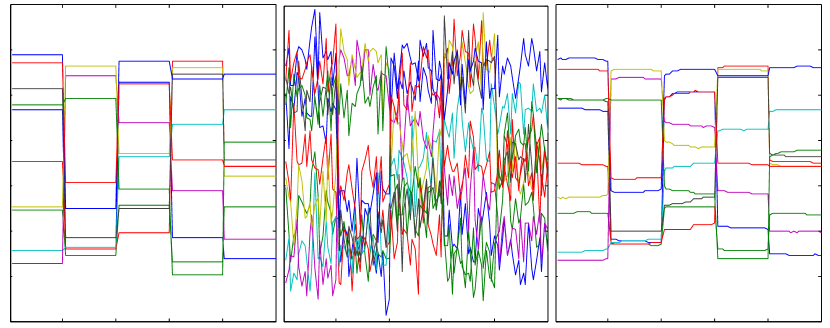
Refer to caption
Figure 5: Illustration of the signal data used in the Fused Lasso experiments. We show the original signal (left), the noisy signal given to the algorithm (middle), and the signal recovered after performing the fused lasso optimization (right).

D.4 Comparison to parallel block coordinate descent

With some understanding on Cfτsuperscriptsubscript𝐶𝑓𝜏C_{f}^{\tau}, we can now explicitly compare the rate of convergence in Theorem 1 with parallel BCD [36, 30] under the assumption of μ=O(B/τ)𝜇𝑂𝐵𝜏\mu=O(B/\tau) — a fair and equally favorable case to all of these methods. To facilitate comparison, we will convert the constants in all three methods to block coordinate gradient Lipschitz constant Lisubscript𝐿𝑖L_{i}, which obeys

f(x+s[i])f(x)+s[i],f(x)+Lis[i]2,𝑓𝑥subscript𝑠delimited-[]𝑖𝑓𝑥subscript𝑠delimited-[]𝑖𝑓𝑥subscript𝐿𝑖superscriptnormsubscript𝑠delimited-[]𝑖2f(x+s_{[i]})\leq f(x)+\langle s_{[i]},\nabla f(x)\rangle+L_{i}\|s_{[i]}\|^{2}, (22)

for any x,s(i)iformulae-sequence𝑥subscript𝑠𝑖subscript𝑖x\in\mathcal{M},s_{(i)}\in\mathcal{M}_{i}. Observe that Bisubscript𝐵𝑖B_{i} \leq 4Lidiam(i)24subscript𝐿𝑖diamsuperscriptsubscript𝑖24L_{i}\mathrm{diam}(\mathcal{M}_{i})^{2} == Limaxxi,xiixixi2subscript𝐿𝑖subscriptsuperscriptsubscript𝑥𝑖subscript𝑥𝑖subscript𝑖superscriptnormsubscript𝑥𝑖subscriptsuperscript𝑥𝑖2L_{i}\max_{x_{i}^{*},x_{i}\in\mathcal{M}_{i}}\|x_{i}-x^{*}_{i}\|^{2}, so

B𝐵\displaystyle B 1niLimaxxi,xixixiabsent1𝑛subscript𝑖subscript𝐿𝑖subscriptsubscript𝑥𝑖subscriptsuperscript𝑥𝑖normsubscript𝑥𝑖subscriptsuperscript𝑥𝑖\displaystyle\leq\frac{1}{n}\sum_{i}L_{i}\max_{x_{i},x^{*}_{i}}\|x_{i}-x^{*}_{i}\| (23)
1niLimaxxxx2=𝔼i(Li)R2absent1𝑛subscript𝑖subscript𝐿𝑖subscript𝑥superscriptnorm𝑥superscript𝑥2subscript𝔼𝑖subscript𝐿𝑖superscript𝑅2\displaystyle\leq\frac{1}{n}\sum_{i}L_{i}\max_{x}\|x-x^{*}\|^{2}=\mathbb{E}_{i}(L_{i})R^{2} (24)

where R:=maxxxxassign𝑅subscript𝑥norm𝑥superscript𝑥R:=\max_{x}\|x-x^{*}\|. The rate of convergence for the three methods (with τ𝜏\tau oracle calls considered as one iteration) are given below.

Method Rate
Ap-Bcfw (Ours) Op(n𝔼i(Li)R2τk)subscript𝑂𝑝𝑛subscript𝔼𝑖subscript𝐿𝑖superscript𝑅2𝜏𝑘O_{p}\left(\frac{n\mathbb{E}_{i}(L_{i})R^{2}}{\tau k}\right)
P-BCD555In Richtárik & Takáč [36, Theorem 19] Op(n𝔼i(Li)R2τk)subscript𝑂𝑝𝑛subscript𝔼𝑖subscript𝐿𝑖superscript𝑅2𝜏𝑘O_{p}\left(\frac{n\mathbb{E}_{i}(L_{i})R^{2}}{\tau k}\right)
AP-BCD666In Liu et al. [30, Theorem 3] Op(nmaxiLiR2τk)subscript𝑂𝑝𝑛subscript𝑖subscript𝐿𝑖superscript𝑅2𝜏𝑘O_{p}\left(\frac{n\max_{i}L_{i}R^{2}}{\tau k}\right)

The comparison illustrates that these methods have the same O(1/k)𝑂1𝑘O(1/k) rate and almost the same dependence on n𝑛n and τ𝜏\tau despite the fact that we use a much simpler linear oracle. Nothing comes for free though: Nesterov acceleration does not apply for Frank-Wolfe based methods in general, while a careful implementation of parallel coordinate descents can achieve O(1/k2)𝑂1superscript𝑘2O(1/k^{2}) rate without any full-vector interpolation in every iteration [11]. Also, Frank-Wolfe methods usually need additional restrictive conditions or algorithmic steps to get linear convergence for strongly convex problems.

These facts somewhat limits the applicability of our method to cases when projection can be computed as efficiently as (3). However, as is surveyed in [21], there are many interesting cases when (3) is much cheaper than projections, e.g., projection onto a nuclear norm ball takes O(n3)𝑂superscript𝑛3O(n^{3}) while (3) takes only O(n2)𝑂superscript𝑛2O(n^{2}).