Quantum Gravity Effect in Torsion Driven Inflation and CP violation

Abstract

We have derived an effective potential for inflationary scenario from torsion and quantum gravity correction in terms of the scalar field hidden in torsion. A strict bound on the CP violating $\theta$ parameter, ${\cal O}(10^{-10})<\theta<{\cal O}(10^{-9})$ has been obtained, using Planck+WMAP9 best fit cosmological parameters.

I Introduction

The paradigm of cosmic inflation complements the big-bang theory and when combined together it is the best theory compatible with the latest observations. Inflation is generally believed to be driven by a scalar field known as inflaton. Gasperini gasperini has pointed out that the inflationary scenario can be well explained through torsion . Later, Poplawski pop1 have argued that torsion can be treated as an alternative source of inflation. In this context, it is also to be noted that when torsion is considered to be generated from spin-spin interaction a hidden scalar field can be associated with torsion mullick . It is interesting to know whether the associated scalar field in torsion plays the role of inflaton in the inflationary regime such that ”the scalar field driven inflation” as well as the ”torsion driven inflation” appear to be equivalent statements. The motivation of the present paper is to show that if in the Einstein-Cartan-Kibble-Sciama (ECKS) theory of gravity, the quantum gravity effect in the early universe is taken into account, we can formulate an effective potential for inflation in terms of the scalar field hidden in the torsion. Besides, the formulation gives rise to a CP violating term. The estimate of the bound on CP violation in the early Universe using Planck+WMAP9 best fit cosmological parameters Ade:2013uln has also been obtained.

II Torsion induced potential

To study torsion in terms of the spin-spin interaction we take resort to a spin-current duality relation so that the action for torsion can be developed through a dual current-current interaction. We consider a four vector $n_{\mu}$ in terms of the spinorial variables as

$$n_{\mu}=\left(\frac{1}{\sqrt{2}}\right)(\psi_{1}^{*}~{}~{}~{}\psi_{2}^{*})\sigma_{\mu}\left(\begin{array}[]{c}\psi_{1}\\ \psi_{2}\end{array}\right)$$ (1)

where

$$\psi_{1}=(\cos\theta/2)e^{i\phi/2},~{}~{}~{}\psi_{2}=(\sin\theta/2)e^{-i\phi/2},$$ (2)

with $\sigma_{0}=I$, where $I$ is the identity matrix and $\vec{\sigma}$ is the vector of Pauli matrices. Using this one can construct an SU(2) group element

$$g=n_{0}I+i~{}\vec{\bf n}.\vec{\bf{\sigma}},$$ (3)

in terms of which we can construct the topological current as Abanov:1999qz :

$$J_{\mu}=\left(\frac{1}{24\pi^{2}}\right)\epsilon_{\mu\nu\lambda\sigma}{\rm Tr}[(g^{-1}\partial^{\nu}g)(g^{-1}\partial^{\lambda}g)(g^{-1}\partial^{\sigma}g)]$$ (4)

where $\epsilon_{\mu\nu\lambda\sigma}$ is the rank-4 Levi-Civita tensor. Now by demanding that in 4-dimensional Euclidean space the field strength $F_{\mu\nu}$ of a gauge potential vanishes on the boundary $S^{3}$ of a certain volume ${\rm Vol_{4}}$ inside of which $F_{\mu\nu}\neq 0$, we can write the gauge potential as $A_{\mu}=g^{-1}\partial_{\mu}g\in{\bf SU(2)}$. Then from Eq.(4) the Kac-Moody like current $J_{\mu}$ can be recast in terms of the Chern-Simons secondary characteristic class as cs :

$$J_{\mu}=\left(\frac{1}{16\pi^{2}}\right)\epsilon^{\mu\nu\lambda\sigma}{\rm Tr}\left(A_{\nu}F_{\lambda\sigma}+\frac{2}{3}A_{\nu}A_{\lambda}A_{\sigma}\right)$$ (5)

This gives rise to a topological invariant :

$$Q_{P}=\left(\frac{1}{16\pi^{2}}\right)\int d^{4}x~{}\partial_{\mu}J^{\mu}$$ (6)

which is known as the Pontryagin index. We can construct the Lagrangian from the divergence of the current $J_{\mu}$ and write

$${\cal L}=-\frac{1}{4}{\rm Tr}\left(\epsilon_{\mu\nu\lambda\sigma}F^{\mu\nu}F^{\lambda\sigma}\right)$$ (7)

which leads to the construction of the current carmeli

$${\bf{j}}^{\mu}=\epsilon^{\mu\nu\lambda\sigma}{\bf a}_{\nu}\otimes{\bf f}_{\lambda\sigma}=\epsilon^{\mu\nu\lambda\sigma}\partial_{\nu}{\bf f}_{\lambda\sigma}$$ (8)

with $A_{\mu}={\bf a}_{\mu}.{\bf{\sigma}}$ and

$$F_{\mu\nu}=\partial_{[\mu}A_{\nu]}+[A_{\mu},A_{\nu}]={\bf f}_{\mu\nu}.{\bf{\sigma}}$$ (9)

It can be shown that the axial vector current

$$J_{\mu}^{5}=\bar{\psi}\gamma_{\mu}\gamma_{5}\psi$$ (10)

is related to the second component of the current ${\bf j}_{\mu}$ through the relation

$$\partial^{\mu}j_{\mu}^{(2)}=-\frac{1}{2}\partial^{\mu}J_{\mu}^{5}\neq 0.$$ (11)

The consistency of the current conservation equations implies that aroy :

$$j_{\mu}^{(1)}=-\frac{1}{2}j_{\mu}^{(2)},j_{\mu}^{(3)}=+\frac{1}{2}j_{\mu}^{(2)}$$ (12)

Consequently, the current-current interaction can be expressed in terms of $j_{\mu}^{(2)}$ only which effectively displays the spin-spin interaction. Now we can write the action for torsion as aban

$$S_{T}=\frac{M^{2}_{p}}{2}\int J_{\mu}^{2}J_{\mu}^{2}d^{4}x$$ (13)

where $M_{p}$ being the reduced Planck mass, given by $M_{p}\approx 2.43\times 10^{18}$ GeV. It is now observed that there is a hidden scalar field $\phi$ in torsion which follows from the relation

$${j}^{\mu(2)}=\epsilon^{\mu\nu\lambda\sigma}\partial_{\nu}{f}_{\lambda\sigma}^{(2)}=\epsilon^{\mu\nu\lambda\sigma}{\epsilon}_{\nu\lambda\sigma}\phi(x)$$ (14)

where ${\epsilon}^{\nu\lambda\sigma}$ is the rank-3 Levi-Civita tensor. The action now turns out to be:

$$\small S_{T}={\cal A}\int d^{4}x~{}j_{\mu}^{(2)}j^{\mu~{}(2)}=\int d^{4}x~{}\sqrt{-g_{(4)}}~{}\frac{m^{2}}{2}\phi^{2}$$ (15)

Eq.(15) suggests that the potential associated with torsion can be written as:

$$V_{T}(\phi)=-\frac{m^{2}}{2}\phi^{2}.$$ (16)

The negative sign of the coupling constant $m^{2}$ actually corresponds to the self interaction, when orientation of all the spin degrees of freedom are along the same direction.

III INFLATIONARY MODELING WITH THE CP VIOLATING TERM

Now we analyse the contribution from quantum gravity. To this end we utilize the model of Capovilla, Jacobson and Drell (CJD) cjd , where the action is given by cjd :

$$S=\frac{1}{8}\int\eta(\Omega_{ij}\Omega_{ij}+a\Omega_{ii}\Omega_{jj})$$ (17)

where

$$\Omega_{ij}=\epsilon^{\alpha\beta\gamma\delta}F_{\alpha\beta i}F_{\gamma\delta j}$$ (18)

with $\alpha,\beta,\gamma,\delta$ as space time indices, $i,j$ the ${\bf SU(2)}$ group indices and $\eta$ is a scalar density. In Ref. cjd it has been shown that in 3+1 decomposition this action yields Ashteker action directly provided we have $a=-\frac{1}{2}$ and the determinant of the magnetic field ${B^{i}}_{a}$ is non zero and as such the equivalence to the Einstein’s theory is established. The equivalence to the Einstein’s theory can also be shown when the space time metric is found to be given by

$$\sqrt{-g_{(4)}}g^{\alpha\beta}=-\left(\frac{2i}{3\eta}\right)\epsilon_{ijk}\epsilon^{\alpha\gamma\delta\rho}\epsilon^{\beta\mu\nu\sigma}F_{\gamma\delta i}F_{\rho\sigma j}F_{\mu\nu k}$$ (19)

The constraint that is obtained when the CJD action is varied with respect to the Lagrangian multiplier $\eta$ is actually the Hamiltonian constraint

$$\Psi=\Omega_{ij}\Omega_{ij}~{}-~{}\frac{1}{2}\Omega_{ii}\Omega_{jj}=i(2\eta^{2}~{}detB)^{-1}~{}H$$ (20)

This implies that $\Psi\approx 0$ and $H\approx 0$ are equivalent statements provided $detB\neq 0$. The canonical transformation of SU(2) gauge potential ($A_{ai}$) and the corresponding non-abelian fields ($E_{i}^{a},B_{i}^{a}$):

$$A_{ai} \rightarrow A_{ai},$$ (21)

$$E_{i}^{a} \rightarrow E_{i}^{a}-\theta B_{i}^{a}$$ (22)

gives rise to a CP-violating $\theta$ term in the CJD Lagrangian so that for $a=-1/2$ the action now reads cjd ; mullick ; pratul :

$$S_{C}=\frac{1}{8}\int\left[\theta\Omega_{ii}~{}+~{}\eta\left(\Omega_{ij}\Omega_{ij}-\frac{1}{2}\Omega_{ii}\Omega_{jj}\right)\right].$$ (23)

In the first term the parameter $\theta$ essentially corresponds to the measure of CP violation which contributes to torsion and the rest is curvature contribution. Consequently Eq.(23) can be recast as:

$$S_{C} = -\frac{\theta}{4}Q_{P}+\eta\int d^{4}x~{}\epsilon^{\alpha\beta\gamma\delta}\epsilon^{\lambda\rho\sigma\mu}\epsilon_{\nu\alpha\beta}\epsilon_{\nu^{{}^{\prime}}\lambda\rho}\epsilon_{\xi\nu\delta}\epsilon_{\xi^{{}^{\prime}}\sigma\mu}\int dx^{\nu}~{}\phi\int dx^{\nu^{{}^{\prime}}}~{}\phi\int dx^{\xi}~{}\phi\int dx^{\xi^{{}^{\prime}}}~{}\phi$$ (24)

$$~{}~{}~{}~{}~{}~{}~{}~{}~{}~{}~{}~{}~{}~{}~{}~{}~{}~{}~{}~{}~{}~{}~{}~{}~{}~{}~{}~{}~{}~{}~{}~{}~{}~{}~{}~{}~{}~{}~{}~{}~{}~{}~{}~{}~{}~{}~{}~{}~{}~{}~{}~{}~{}~{}~{}~{}~{}-\frac{\eta}{2}\int d^{4}x~{}\epsilon^{\mu\nu\lambda\sigma}\epsilon^{\alpha\beta\gamma\delta}\epsilon_{\nu\lambda\sigma}\epsilon_{\beta\gamma\delta}~{}(\partial_{\mu}\phi)(\partial_{\alpha}\phi)$$

where $\int dx^{\nu}~{}\phi=\phi~{}[x^{\nu}]$, and the symbol $[\cdots]$ signifies the boundary value of the coordinates in the affine parameter space. Now from Eq.(24) we get :

$$\small S_{C}=-\frac{\theta}{4}Q_{P}+\int d^{4}x\sqrt{-g_{(4)}}\left[\frac{g^{\mu\alpha}}{2}(\partial_{\mu}\phi)(\partial_{\alpha}\phi)-\frac{\lambda}{4}\phi^{4}\right].$$ (25)

It may be mentioned here that the first term on the right hand side incorporates the Pontryagin index given by Eq.(6) which is a topological term arising from a total divergence. This does not contribute classically but has the effect in the quantum mechanical formulation.

From Eq (15) and Eq (25), we note that the action for torsion (curvature) when expressed in terms of the $\phi$ field involves the term $\phi^{2}(\phi^{4})$. This indicates that the anisotropies associated with the torsion are much suppressed in comparison to the contribution from curvature for large values of $\phi$. It is noted that the the expression of curvature in terms of the scalar field arises when we use CJD Lagrangian. In this sense the scalar field does not arise from gravitation as such, but it originates from the torsional degrees of freedom associated with the spin density.

Noting that the asymptotic constancy of torsion compensates the bare cosmological constant Baekler:1987jb we can define a small but non-vanishing cosmological constant in terms of the Pontryagin index as

$$M_{p}^{2}\Lambda_{eff}=\frac{\theta}{8~{}\rm Vol_{4}}Q_{P}$$ (26)

where $M_{p}$ coresponds to the Planck mass. We can define the vacuum energy $V_{0}$ through the relation

$$V_{0}=3H^{2}_{inf}\Lambda^{2}_{UV}=\Lambda_{eff}\Lambda^{2}_{UV}$$ (27)

Here $\Lambda_{UV}$ signifies the UV cut-off scale of the proposed EFT theory . Below $\Lambda_{UV}$ the effect of all quantum corrections are highly suppressed and the heavy fields from the hidden sector gets their VEV. Such VEV is one of the possible sources of vacuum energy correction in the spin-current dominated EFT picture which uplifts the scale of inflationary potential and the contributions of the VEV become significant upto a scale $\Lambda_{C}\leq\Lambda_{UV}$. But at very low scale, $\Lambda_{low}\ll\Lambda_{C}$, one can tune the vacuum energy correction, $V_{0}\approx 0$ for which the contributions of the VEV can be neglected Allahverdi:2006iq . Such possibility is only significant when the contribution of the primordial gravity waves become negligibly small (see Eq.(34)). Thus the expression for the potential from CJD Lagrangian incorporating the CP violating $\theta$ term yields:

$$V_{C}(\phi)=V_{0}+\frac{\lambda}{4}\phi^{4}.$$ (28)

IV The effective potential

Now in the background of a space-time manifold having Riemannian structure the contribution to the conserved current can be expressed as:

$$J^{\mu~{}g}=\frac{1}{2}\epsilon^{\mu\nu\lambda\sigma}R_{\nu\lambda\sigma\delta}v^{\delta},$$ (29)

where $v^{\delta}$ is an arbitrary vector and Riemann curvature tensor can be expressed as:

$$R_{\nu\lambda\sigma\delta}=\partial_{[\lambda}\omega_{\nu]\sigma\delta}+\omega^{\eta}_{\nu\sigma}\omega_{\lambda\eta\delta}-\omega^{\xi}_{\lambda\sigma}\omega_{\nu\xi\delta}-e_{\sigma\nu}e_{\delta\lambda}.$$ (30)

As a result the gravitational part of the action can be written in terms of gravitational current-current interaction in the Riemann space as:

$$\small S_{g}=-\frac{\Lambda^{2}_{UV}}{2}\int d^{4}xJ_{\mu}^{g}J^{\mu~{}g}=\frac{\Lambda^{2}_{UV}}{2}\int d^{4}x\sqrt{-g_{4}}R$$ (31)

Now clubbing the contributions from Eqns.(15,25,31) the total action for the present field theoretic setup, taking into account quantum gravity correction, can finally be written as:

$$\displaystyle S=\int d^{4}x\sqrt{-g_{4}}\left[\frac{\Lambda^{2}_{UV}}{2}R+\frac{g^{\mu\alpha}}{2}(\partial_{\mu}\phi)(\partial_{\alpha}\phi)-V(\phi)\right]$$ (32)

such that the total effective potential is given by:

$$V(\phi)=V_{T}(\phi)+V_{C}(\phi)=V_{0}-\frac{m^{2}}{2}\phi^{2}+\frac{\lambda}{4}\phi^{4}.$$ (33)

V Estimate on the CP violation term

The effective potential is dominated by the vacuum energy correction term which determines the scale of inflation. To obtain the scale of inflation at $k_{*}\approx k_{cmb}$, we express $V_{0}$ in terms of inflationary observables as:

$$V^{1/4}_{*}\approx V^{1/4}_{0}=7.389\times 10^{-3}\Lambda_{UV}\times\left(\frac{r}{0.1}\right)^{1/4}.$$ (34)

where $r$ is the tensor-to-scalar ratio defined as: $r=A_{T}/A_{S}$ with $(A_{T},A_{S})$ being the amplitudes of the power spectra for scalar ($S$) and tensor ($T$) modes at $k=aH\approx k_{*}$. The effective cosmological constant or equivalently the CP violating parameter $\theta$ can then be constrained as:

$$\Lambda_{eff}=\frac{\theta}{8~{}Vol_{4}}Q_{P}=2.98\times 10^{-9}\Lambda^{2}_{UV}\times\left(\frac{r}{0.1}\right).$$ (35)

In order to compare the theoretical predictions with the latest observations we use a numerical code CLASS class . In this code we can directly input the shape of the potential along with the model parameters. Then for a given cosmological background the code provides the estimates for different CMB observables. In the code we set the momentum pivot at $k_{*}=0.05$ Mpc^-1 and used the Planck + WMAP9 best fit values:

$$h=0.670,~{}~{}\Omega_{b}=0.049,~{}~{}\Omega_{c}=0.268,~{}~{}\Omega_{\Lambda}=0.682$$ (36)

for background cosmological parameters. In this work we scan the parameter space within the following window:

$$2.501\times 10^{-9}~{}\Lambda^{4}_{UV}\leq V_{0}\leq 2.589\times 10^{-9}~{}\Lambda^{4}_{UV},$$

$$6\times 10^{-3}~{}\Lambda^{-2}_{UV}\leq m^{2}/V_{0}\leq 8\times 10^{-3}~{}\Lambda^{-2}_{UV},$$

$$\lambda/V_{0}\sim 10^{-6}~{}\Lambda^{-4}_{UV}.$$ (37)

As a result, the CMB observables are constrained within the following range:

$$2.197\times 10^{-9} \leq A_{S}\leq 2.202\times 10^{-9},$$

$$0.957 \leq n_{S}\leq 0.962,$$

$$-1.08\times 10^{-3} \leq\alpha_{S}\leq -0.99\times 10^{-3},$$

$$0.055 \leq r\leq 0.057.$$ (38)

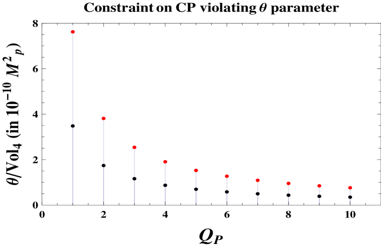
Figure 1: Constraint on CP violating topological $\theta$ parameter for discrete integer values of Pontryagin index $Q_{P}$ using Planck + WMAP9 best fit cosmological parameters. Here Red and black colored points correspond to the upper and lower bound of the $\theta$ parameter for a given value of $Q_{P}$. All the parallel blue colored lines are drawn for different integer values of $Q_{P}$ which connects both the Red and black colored points. This plot suggests that as the value of $Q_{P}$ increases then the interval between the upper and lower bound of the $\theta$ parameter decrease and it will converge to very small value for large $Q_{P}$. Also the numerical value corresponding to the upper bound and lower bound of the $\theta$ parameter decreases once we increase the the value of $Q_{P}$.

Within the present context the field excursion Lyth:1996im ; Choudhury:2013iaa ; Baumann:2011ws is defined as:

$$\left|\Delta\phi\right|=\Lambda_{UV}\int^{N_{cmb}}_{0}dN\sqrt{\frac{r(N)}{8}}\approx\sqrt{\frac{r}{8}}N_{cmb}\Lambda_{UV}.$$ (39)

where $|\Delta\phi|=|\phi_{*}-\phi_{f}|$, in which $\phi_{*}$ and $\phi_{f}$ represent the field value corresponding to CMB scale and end of inflation respectively. Also $N_{cmb}$ is the number of e-foldings at CMB scale which is fixed at $N_{cmb}\approx 50-70$ to solve the horizon problem associated with inflation. Subsequently we get the following constraint on the field excursion:

$$\left|\Delta\phi\right|\sim{\cal O}(4.1-5.9)\times\Lambda_{UV},$$ (40)

which implies to make the EFT of inflation validate within the prescribed setup for which we need to constrain the UV cut-off of the EFT within the following window:

$$\Lambda_{UV}\sim{\cal O}(0.16-0.24)~{}M_{p}<M_{p},$$ (41)

which is just below the scale of reduced Planck mass. Finally using Eq.(35) we get the following bound on the CP violating parameter  :

$$3.48\times 10^{-10}M^{2}_{p}\leq\frac{\theta}{Vol_{4}}Q_{P}\leq 7.62\times 10^{-10}M^{2}_{p}.$$ (42)

VI Discussion

Thus once we fix $Q_{P}$, this will further provide an estimate of $\theta$ according to the Eq.(42). In Fig. (1) we have explicitly shown the constraint on $\theta$ from the proposed EFT picture which is obtained by using Planck + WMAP9 best fit cosmological parameters. To exemplify we have prescribed the bound on $\theta$ for different integer values of $Q_{P}$ lying within $1\leq Q_{P}\leq 10$. From the plot it is easy to see that as the value of $Q_{P}$ increases the bound on the parameter $\theta$ converges to a very small value. This suggests that $\theta$ will converge to a constant value beyond a certain value of $Q_{P}$. It may be mentioned that the Pontryagin index can be taken to correspond to the fermion number Pratul1992 . Indeed a fermion can be realized as a scalar particle encircling a vortex line which is topologically equivalent to a magnetic flux line and thus represents a skyrmion Pratul1992 . The monopole charge $\mu=1/2$ corresponding to a magnetic flux line is related to the Pontryagin index through the relation $Q_{P}=2\mu$. In view of this, one may note that $Q_{P}$ represents the fermion number which is the topological index carried by a fermion. For an anti-fermion $Q_{P}$ takes the negative value. In any system the effective fermion number is given by the difference between the number of fermions and anti-fermions. Thus we can quantify the fermionic matter and hence the spin density through the total accumulated value of $Q_{P}$. As $Q_{P}$ increases we have the increase of fermions implying the increase in spin density. So from Eq.(42) we note that for a fixed volume when $Q_{P}$ increases indicating the increase in spin density, the bound on the parameter $\theta$ converges to a small value representing the residual effect of torsion residing at the boundary. Thus the remnant of CP violation  giving rise to torsion can be witnessed through the small value of $\theta$ which is operative at the boundary.

To summarize, we have derived an effective potential for inflationary scenario, taking into account the quantum gravity effect, in terms of the hidden scalar field associated with torsion along with a CP violating term.Using this we give an estimate of inflationary CMB observables by constraining the model parameters- vacuum energy, mass and self-coupling from Planck + WMAP9 best fit values of the cosmological parameters. Finally, for the first time we constrain the CP violating topological $\theta$ parameter from the vacuum energy correction within EFT.

Acknowledgments: SC would like to thank Department of Theoretical Physics, Tata Institute of Fundamental Research, Mumbai for providing me Visiting (Post-Doctoral) Research Fellowship. SC take this opportunity to thank sincerely to Prof. Sandip P. Trivedi, Prof. Shiraz Minwalla, Prof. Soumitra SenGupta, Prof. Sudhakar Panda, Prof. Varun Sahni, Prof. Sayan Kar, Prof. Sudhakar Panda, Dr. Subhabrata Majumdar and Dr. Supratik Pal for their constant support and inspiration. SC take this opportunity to thank all the active members and the regular participants of weekly student discussion meet “COSMOMEET” from Department of Theoretical Physics and Department of Astronomy and Astrophysics, Tata Institute of Fundamental Research for their strong support. Last but not the least, we would all like to acknowledge our debt to the people of India for their generous and steady support for research in natural sciences, especially for theoretical high energy physics, string theory and cosmology.

References

- (1) M. Gasperini, Phys. Rev. Lett. 56 (1986) 2873.
- (2) S. Alexander, T. Biswas and G. Calcagni, Phys. Rev. D 81 (2010) 043511 [Phys. Rev. D 81 (2010) 069902] [arXiv:0906.5161 [astro-ph.CO]].
- (3) Nikodem J. Poplawski, Phys. Lett. B 694 (2010) 181 [arXiv:1007.0587 [astro-ph.CO]].
- (4) L. Mullick and P. Bandyopadhyay, J. Math. Phys. 36 (1995) 370.
- (5) P. A. R. Ade et al. [Planck Collaboration], arXiv:1303.5082 [astro-ph.CO]; P. A. R. Ade et al. [Planck Collaboration], Astron. Astrophys. (2014) [arXiv:1303.5076 [astro-ph.CO]].
- (6) A. G. Abanov and P. B. Wiegmann, Nucl. Phys. B 570 (2000) 685 [hep-th/9911025].
- (7) S. S. Chern and J. Simons, Annals of Maths. 99 (1974) 48.
- (8) M. Carmeli and S. Malin, Annals of Phys. (N.Y.) 103 (1977) 208.
- (9) A. Roy and P. Bandyopadhyay, J. Math. Phys. 30 (1989) 2366;
- (10) A. Bandyopadhyay, P. Chatterjee and P. Bandyopadhyay, Gen. Rel. Grav. 18 1293 (1986)
- (11) R. Capovilla, T. Jacobson and J. Dell, Phys. Rev. Lett. 63 (1989) 2325; R. Capovilla, T. Jacobson and J. Dell, Class. Quantum Grav. 8 (1991) 59.
- (12) I. Bengtsson and P. Peldan. Phys. Lett. B, 244 (1990) 261; I. Bengtsson and P. Peldan. Int. J. Mod. Phys. A, 7 (1992) 1287;
- (13) P. Baekler, E. W. Mielke, R. Hecht and F. W. Hehl, Nucl. Phys. B 288 (1987) 800.
- (14) R. Allahverdi, K. Enqvist, J. Garcia-Bellido and A. Mazumdar, Phys. Rev. Lett. 97 (2006) 191304 [hep-ph/0605035]; S. Choudhury, A. Mazumdar and S. Pal, JCAP 1307 (2013) 041 [arXiv:1305.6398 [hep-ph]].
- (15) V. Assassi, D. Baumann, D. Green and L. McAllister, arXiv:1304.5226 [hep-th]; D. Baumann and L. McAllister, arXiv:1404.2601 [hep-th].
- (16) S. Choudhury, A. Mazumdar and E. Pukartas, JHEP 1404 (2014) 077 [arXiv:1402.1227 [hep-th]]; S. Choudhury, JHEP 1404 (2014) 105 [arXiv:1402.1251 [hep-th]].
- (17) S. Choudhury and S. Sengupta, JHEP 1302 (2013) 136 [arXiv:1301.0918 [hep-th]]; S. Choudhury and S. SenGupta, arXiv:1306.0492 [hep-th]; S. Choudhury, J. Mitra and S. SenGupta, JHEP 1408 (2014) 004 [arXiv:1405.6826 [hep-th]]; S. Choudhury and S. SenGupta, Eur. Phys. J. C 74 (2014) 11, 3159 [arXiv:1311.0730 [hep-ph]]; S. Choudhury, J. Mitra and S. SenGupta, arXiv:1503.07287 [hep-th].
- (18) T. Biswas, E. Gerwick, T. Koivisto and A. Mazumdar, Phys. Rev. Lett. 108 (2012) 031101 [arXiv:1110.5249 [gr-qc]].
- (19) V. Assassi, D. Baumann and D. Green, JHEP 1302 (2013) 151 [arXiv:1210.7792 [hep-th]]; L. Senatore and M. Zaldarriaga, JHEP 1012 (2010) 008 [arXiv:0912.2734 [hep-th]]; L. Senatore and M. Zaldarriaga, JHEP 1301 (2013) 109 [JHEP 1301 (2013) 109] [arXiv:1203.6354 [hep-th]]; G. L. Pimentel, L. Senatore and M. Zaldarriaga, JHEP 1207 (2012) 166 [arXiv:1203.6651 [hep-th]].
- (20) CLASS: The Cosmic Linear Anisotropy Solving System: http://class-code.net/.
- (21) D. H. Lyth, Phys. Rev. Lett. 78 (1997) 1861 [hep-ph/9606387].
- (22) S. Choudhury and A. Mazumdar, Nucl. Phys. B 882 (2014) 386 [arXiv:1306.4496 [hep-ph]]; S. Choudhury and A. Mazumdar, arXiv:1403.5549 [hep-th]; S. Choudhury and A. Mazumdar, arXiv:1404.3398 [hep-th]; S. Choudhury, arXiv:1406.7618 [hep-th]; S. Choudhury, arXiv:1508.00269 [astro-ph.CO]; S. Choudhury and S. Banerjee, arXiv:1506.02260 [hep-th]; S. Choudhury, arXiv:1504.08206 [astro-ph.CO]; D. Chialva and A. Mazumdar, arXiv:1405.0513 [hep-th].
- (23) D. Baumann and D. Green, JCAP 1205 (2012) 017 [arXiv:1111.3040 [hep-th]].
- (24) V. Parameswaran Nair, Quantum Field Theory: A Modern Perspective, Springer publication, 2005 edition.
- (25) D. Banerjee and P. Bandyopadhyay, J. Math. Phys. 33 (1992) 990; P. Bandyopadhyay, Proc. R. Soc. London A 466 (2010) 2917.
- (26) H. Kodama, Phys. Rev. D. 42 (1990) 2548.