Correlation between centrality metrics and their application to the opinion model

Abstract

In recent decades, a number of centrality metrics describing network properties of nodes have been proposed to rank the importance of nodes. In order to understand the correlations between centrality metrics and to approximate a high-complexity centrality metric by a strongly correlated low-complexity metric, we first study the correlation between centrality metrics in terms of their Pearson correlation coefficient and their similarity in ranking of nodes. In addition to considering the widely used centrality metrics, we introduce a new centrality measure, the degree mass. The $m$th-order degree mass of a node is the sum of the weighted degree of the node and its neighbors no further than $m$ hops away. We find that the betweenness, the closeness, and the components of the principal eigenvector are strongly correlated with the degree, the $1$st-order degree mass and the $2$nd-order degree mass, respectively, in both network models and real-world networks. We then theoretically prove that the Pearson correlation coefficient between the principal eigenvector and the $2$nd-order degree mass is larger than that between the principal eigenvector and a lower order degree mass. Finally, we investigate the effect of the inflexible contrarians selected based on different centrality metrics in helping one opinion to compete with another in the inflexible contrarian opinion (ICO) model. Interestingly, we find that selecting the inflexible contrarians based on the leverage, the betweenness, or the degree is more effective in opinion-competition than using other centrality metrics in all types of networks. This observation is supported by our previous observations, i.e., that there is a strong linear correlation between the degree and the betweenness, as well as a high centrality similarity between the leverage and the degree.

1 Introduction

Recent research has explored social dynamics [1, 2, 3] by using complex networks in which nodes represent people/agents and links the associations between them. Such centrality metrics as degree and betweenness have been studied in dynamic processes [4, 5, 6, 7], such as opinion competition, epidemic spreading, and rumor propagation on complex networks. These studies used centrality metrics to identify influential nodes [4, 5, 6], such as the source nodes from which a virus spreads and the nodes with high spreading capacity, as well as to select which nodes are to be immunized when a virus is prevalent [7]. Numerous centrality metrics have been proposed. Degree, betweenness, closeness, and principal eigenvector are the most popular centrality metrics [4, 8, 9, 10, 11, 12, 13]. Several new centrality metrics have been introduced in a number of different fields recently. Kitsak et al. [5] studied the SIS and SIR spreading models on four real-world networks and proposed that the $k$-shell index is a better indicator for the most efficient spreaders (nodes) than degree or betweenness. Reference [14] proposes a new centrality metric—leverage—for identifying neighborhood hubs (the most highly-connected nodes) in functional brain networks. Leverage centrality identifies nodes that are connected to more nodes than their nearest neighbors. In addition to considering these widely-used centrality metrics, we here propose a new centrality metric, degree mass. The $m$th-order degree mass of a node is defined as the sum of the weighted degree of its $m$-hop neighborhood. If the degree of a node and of its neighbors are all high, the node has a high degree mass.

Centrality metrics have been compared in various networks, such as sampled networks, biological networks, food webs, and vocabulary networks in literature [4, 15, 16, 17, 18]. Comin et al. [4] compared the centrality metrics characterizing the performances of nodes in such dynamic processes as virus spreading. Kim and Jeong [15] compared the reliability of rank orders using centrality metrics in sampling networks. The correlations between centrality metrics have been studied in biological networks [16, 17]. However correlations between centrality metrics are still not well understood. If correlations between centrality metrics were better understood, we might be able to rank the nodes in a network by using the centrality metrics with a low computational complexity instead of the ones with a high computational complexity. To investigate the correlation between any two centrality metrics, we compute their Pearson correlation coefficient and their similarity in ranking nodes in both network models and real-world networks. In this work (i) we consider Erdős-Rényi (ER) networks with a binomial degree distribution [19] and scale-free (SF) networks with a power-law degree distribution [20, 21]. Studying these two network models allows us to understand how the degree distribution influences correlations between the centrality metrics. (ii) We further explore correlations in 34 real-world networks with differing numbers of nodes and links. (iii) We theoretically compare the Pearson correlation coefficients between the principal eigenvector and the degree masses.

Recently there has been considerable interest in understanding how two competing opinions [22, 23, 24, 25, 26] evolve in a population. In this work we apply our centrality metrics to an inflexible contrarian opinion (ICO) model [27] in which only two opinions (denoted $A$ and $B$) exist, with the goal of helping one opinion (opinion $B$) as it competes with with the other opinion (opinion $A$). At the initial time, opinions are randomly assigned to all nodes (with a fraction $f$ of nodes holding opinion $A$ and a fraction $1-f$ of nodes holding opinion $B$). At each step, each agent simultaneously and in parallel adopts the opinion of the majority of its nearest neighbors and itself, and if there is a tie, the agent does not change its opinion. After the system reaches a steady state, a fraction $p_{o}$ of agents with opinion $A$ is placed among the inflexible contrarians permanently holding opinion $B$, which can affect the opinion of their nearest neighbors. It is known that the size of the giant component of agents with opinion $A$ can be decreased or even destroyed by the inflexible contrarians [27]. Li et al. [27] have selected the inflexible contrarians in ER and SF networks either randomly or based on degree. Here we choose inflexible contrarians using all the centrality metrics we have considered in both modelled networks and real-world networks. We compare the efficiencies of these centrality metrics in reducing the size of the largest opinion $A$ cluster and find that strongly correlated centrality metrics have approximately the same efficiency in both modelled networks and real-world networks. Thus a high-complexity centrality metric could be approximated by a strongly correlated low-complexity centrality metric.

This paper is organized as follows. In Sec. 2 we introduce the centrality metrics. In Sec. 3 we study the Pearson correlation coefficient and the centrality similarity between any two centrality metrics in both network models and real-world networks. In Sec. 4 the Pearson correlations between the degree masses and the principal eigenvector are theoretically analysed. In Sec. 5 the centrality metrics are applied in choosing the inflexible contrarians in the ICO model and the efficiencies of the centrality metrics are compared.

2 Definition of network centrality metrics

Centrality metrics quantify node properties in a network. Here we first review some centrality metrics that are widely used or have been recently proposed [4, 8, 9, 10, 11, 12, 5, 14, 28]. We then propose a new centrality metric, which we call degree mass. Let $G(\mathcal{N}$, $\mathcal{L})$ be a network, where $\mathcal{N}$ is the set of nodes and $\mathcal{L}$ is the set of links. The number of nodes is denoted by $N=|\mathcal{N}|$ and the number of links by $L=|\mathcal{L}|$. The network $G$ can be represented by an $N\times N$ symmetric adjacency matrix $A$, consisting of elements $a_{ij}$, which are either one or zero depending on whether node $i$ is connected to node $j$ or not. The networks mentioned in this paper are simple, unweighted and do not have self-loops or multiple links.

• Principal eigenvector $x_{1}$

The largest eigenvalue of the adjacency matrix $A$ is $\lambda_{1}$, also called the spectral radius [29]. The principal eigenvector $x_{1}$ corresponding to the spectral radius $\lambda_{1}$ satisfies the eigenvalue equation

$$Ax_{1}=\lambda_{1}x_{1}.$$

Component $j$ of the principal eigenvector is denoted by $(x_{1})_{j}$. The $X_{1}$ is the element in the principal eigenvector that corresponds to a random node.

• Betweenness $B_{n}$

Betweenness was introduced independently by Anthonisse [30] in 1971 and Freeman [9] in 1977. The betweenness of a node $i$ is the number of shortest paths between all possible pairs of nodes in the network that traverse the node

$$b_{ni}=\sum_{s\neq i\neq d\in\mathcal{N}}\frac{\sigma_{sd}(i)}{\sigma_{sd}},$$

where $\sigma_{sd}(i)$ is the number of shortest paths that pass through node $i$ from node $s$ to node $d$, and $\sigma_{sd}$ is the total number of shortest paths from node $s$ to node $d$. The betweenness $B_{n}$ incorporates global information and is a simplified quantity for assessing the traffic carried by a node. Assuming that a unit packet is transmitted between each node pair, the betweenness $b_{ni}$ is the total number of packets passing through node $i$ [31].

• Closeness $C_{n}$

The closeness [32] of a node $i$ is the average hopcount of the shortest paths from node $i$ to all other nodes. It measures how close a node is to all the others. The most commonly used definition is the reciprocal of the total hopcount,

$$c_{ni}=\frac{N-1}{\sum_{j\in\mathcal{N}\setminus\{i\}}H_{ij}},$$

where $H_{ij}$ is the hopcount of the shortest path between nodes $i$ and $j$, and $\sum_{j\in\mathcal{N}\setminus\{i\}}H_{ij}$ is the sum of the hopcount of the shortest paths from node $i$ to all other nodes. Closeness has been used to identify central metabolites in metabolic networks [33].

• $K$-shell index $K_{s}$

The $k$-shell decomposition of a network allows us to identify the core and the periphery of the network. The $k$-shell decomposition proceedure is as follows:

• Remove all nodes of degree $d=1$ and also their links. This may reduce the degree of other nodes to 1.

• Remove nodes whose degree has been reduced to 1 and their links until all of the remaining nodes have a degree $d>1$. All of the removed nodes and the links between them constitute the $k$-shell with an index $k_{s}=1$.

• Remove nodes with degree $d=2$ and their links in the remaining networks until all of the remaining nodes have a degree $d>2$. The newly removed nodes and the links between them constitute the k-shell with an index $k_{s}=2$, and subsequently for higher values of $k_{s}$.

The $k$-shell is a variant of the $k$-core [34, 35], which is the largest subgraph with minimum degree of at least $k$. A $k$-core includes all $k$-shells with an index of $k_{s}=0,1,2,\cdots,k$. An $O(m)$ algorithm for $k$-shell network decomposition was proposed in Ref. [36]. The $k$-shell index of the original infected node is a better predictor of the infected population in the susceptible-infectious-recovered (SIR) epidemic spreading process than other centrality metrics, such as the degree [5].

• Leverage $L_{n}$

Joyce et al. [14] introduced leverage centrality in order to identify neighborhood hubs in functional brain networks. The leverage measures the extent of the connectivity of a node relative to the connectivity of its nearest neighbors. The leverage of a node $i$ is defined

$$l_{ni}=\frac{1}{d_{i}}\sum_{j\in\mathcal{N}_{i}}\frac{d_{i}-d_{j}}{d_{i}+d_{j}},$$

where $\mathcal{N}_{i}$ is the directly connected neighbors of the node $i$. With the definition of $l_{ni}$ and the range $[1,N-1]$ of the degree $d_{i}$ in connected networks, the leverage of a node $i$ is bounded by $-1+\frac{2d_{i}}{d_{i}+(N-1)}\leq l_{ni}\leq 1-\frac{2}{d_{i}+1}$. Hence the range of the leverage $l_{ni}$ is $[-1+2/N,1-2/N]$ and the equality occurs in star graphs and complete graphs $K_{N}$. The leverage of a node is high when it has more connections than its direct neighbors. Thus a high-degree node with high-degree nearest neighbors will probably have a low leverage.

• Degree mass $D^{(m)}$

The degree of a node $i$ in a network $G$ is the number of its direct neighbors,

$$d_{i}=\sum_{j=1}^{N}a_{ij}=(Au)_{i},$$

where $u=(1,1,\cdots,1)^{T}$ is the all-one vector. Here we propose a new set of centrality metrics, the degree mass, which is a variant of degree centrality. The $m$th-order degree mass of a node $i$ is defined as the sum of the weighted degree of its $m$-hop neighborhood,

$$d_{i}^{(m)}=\sum_{k=1}^{m+1}\left(A^{k}u\right)_{i}=\sum_{j=1}^{N}\left(\sum_{k=0}^{m}A^{k}\right)_{ij}d_{j},$$

where $m\geq 0$. The weight of the degree $d_{j}$ is the number of walks of length no longer than $m$ from node $i$ to node $j$. The weight of $d_{j}$ is larger than the weight of $d_{l}$ when node $l$ is farther than node $j$ from node $i$. The $m$th-order degree mass vector is defined $d^{(m)}=[d_{1}^{(m)},d_{2}^{(m)},\cdots,d_{N}^{(m)}]$. The 0th-order degree mass is the degree centrality. The 1st-order degree mass of node $i$ is the sum of the degree of node $i$ and the degree of its nearest neighbors. When $m$ is large, the $m$th-order degree mass is proportional to the principal eigenvector.

3 Correlations between centrality metrics

We investigate the correlations between the centrality metrics introduced in Sec. 2, in both network models and real-world networks. The network models include the Erdős-Rényi (ER) network and the scale-free (SF) network. ER networks are characterized by a binomial degree distribution with $\mathrm{Prob}\left[D=k\right]=\binom{N-1}{k}p^{k}(1-p)^{N-1-k}$, where $N$ is the number of nodes and $p$ is the probability that each node pair is connected. A SF network [20, 37] has a power-law degree distribution with Prob$[D=k]\sim k^{-\alpha}$, $k\in\left[k_{\rm min},k_{\rm max}\right]$, where $k_{\rm min}$ is the smallest degree, $k_{\rm max}$ is the degree cutoff, and $\alpha$ is the exponent characterizing the broadness of the distribution. In this work we use the natural cutoff at approximately $N^{1/(\alpha-1)}$ and $k_{\rm min}=2$. We consider 34 real-world networks, e.g., airline connections, electrical power grids, and coauthorship collaborations. The descriptions and properties of these real-world networks are given in Appendix $A$. We study the correlations between any two centrality metrics using the Pearson correlation coefficient and the centrality similarity.

3.1 Pearson correlation coefficients between centrality metrics

Here we explore the linear correlation between the centrality metrics using numerical simulations in both ER and SF networks as well as in real-world networks. The results in Appendix $B$ indicate that strong linear correlations do exist between certain centrality metrics in both ER and SF networks, and that network size has little influence on the correlations. Note that the $k$-shell index is weakly correlated with all the other centrality metrics. This might be the case because the $k$-shell indices of all nodes are similar to each other in binomial networks. We note the following seemingly universal relations between the degree masses and three centrality metrics, the principal eigenvector $x_{1}$, the closeness $C_{n}$ and the betweenness $B_{n}$, as

$$\begin{cases}\rho(X_{1},D^{(2)})>\rho(X_{1},D^{(1)})>\rho(X_{1},D),\\ \rho(C_{n},D^{(1)})>\rho(C_{n},D^{(2)})>\rho(C_{n},D),\\ \rho(B_{n},D)>\rho(B_{n},D^{(2)})>\rho(B_{n},D^{(1)}),\\ \end{cases}$$

in most real-world networks (see Figs. 1a, 1b, and 1c). The same results can be found in both ER and SF networks (see Appendix $B$). We theoretically prove the inequality $\rho(X_{1},D^{(2)})>\rho(X_{1},D^{(1)})>\rho(X_{1},D)$ in ER networks in Sec. 4.

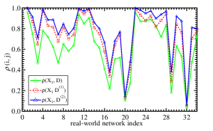
(a)

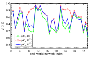
(b)

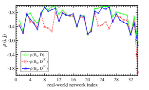
(c)

Figure 1: Pearson correlation coefficients (a) between the principal eigenvector and the degree masses: $\rho(X_{1},D)$ (in circle marks), $\rho(X_{1},D^{(1)})$ (in rectangle marks), and $\rho(X_{1},D^{(2)})$ (in triangle marks); (b) between the closeness and the degree masses: $\rho(C_{n},D)$ (in circle marks), $\rho(C_{n},D^{(1)})$ (in rectangle marks), and $\rho(C_{n},D^{(2)})$ (in triangle marks); (c) between betweenness and degree masses: $\rho(B_{n},D)$ (in circle marks), $\rho(B_{n},D^{(1)})$ (in rectangle marks), and $\rho(B_{n},D^{(2)})$ (in triangle marks), in 34 real-world networks.

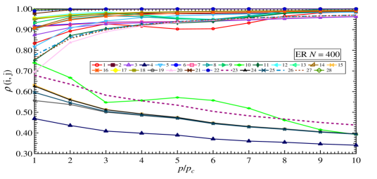
Figure 7: Pearson correlation coefficient between any two centrality metrics as a function of the link density $p$, in ER networks ($N=400$). The number in the annotation is the correlation index.

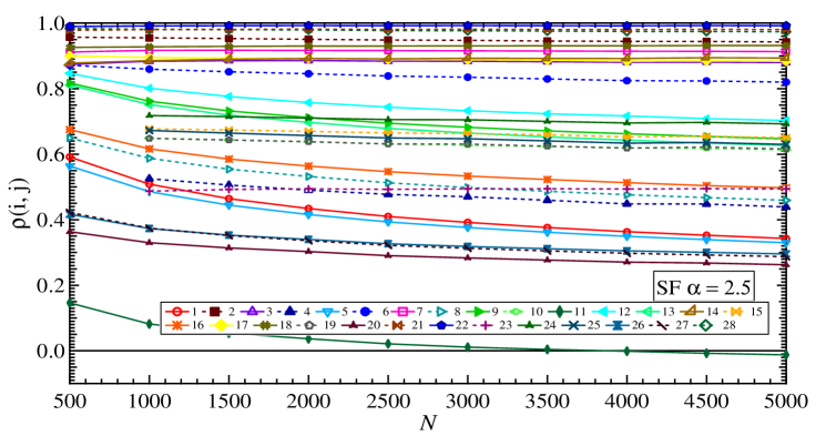
Figure 8: Pearson correlation coefficient between any two centrality metrics as a function of the size $N$ of networks, in scale-free networks ($\alpha=2.5$). The number in the annotation is the correlation index.

Almost all of the Pearson correlation coefficients $\rho(X_{1},D^{(2)})$, $\rho(C_{n},D^{(1)})$, and $\rho(B_{n},D)$ are large ($>0.95$) in both ER and SF networks (see Figs. 7 and 8) and are also large ($>0.6$) in most real-world networks (see Fig. 1). The betweenness of a power-law distributed network also follows a power-law distribution [38]. This supports the strong linear correlation between the betweenness $B_{n}$ and the degree $D$ in SF networks [17].

3.2 Centrality similarities $M_{A,B}(\Upsilon)$ between centrality metrics

Different centrality metrics rank the nodes in different orders within a network. The centrality similarity was proposed in Ref. [39] to quantify the similarity of centrality metrics in ranking nodes.

Definition In a graph $G(N,L)$ assume we obtain two node rankings, $[a_{(1)},a_{(2)},\cdots,a_{(N)}]$ and $[b_{(1)},b_{(2)},\cdots,$ $b_{(N)}]$, according to centrality metrics $A$ and $B$, where $a_{(j)}$ or $b_{(j)}$ is the node whose centrality metric $A$ or $B$ is the $j$-th largest in the networks. The centrality similarity $M_{A,B}(\Upsilon)$ is the percentage of the nodes in $[a_{(1)},a_{(2)},\cdots\cdots,a_{(\Upsilon N)}]$, which are also in $[b_{(1)},b_{(2)},\cdots\cdots,b_{(\Upsilon N)}]$, where $\Upsilon\in[0,1]$.

The measure $M_{A,B}(\Upsilon)$ gives the percentage of overlapping nodes from the top $100\Upsilon\%$ of nodes, ranked by the centrality metrics $A$ and $B$, respectively. The range of $M_{A,B}(\Upsilon)$ is between $[0,1]$. If the $100\Upsilon\%$ of nodes chosen by centrality metric $A$ are not at all in the $100\Upsilon\%$ of nodes chosen by centrality metric $B$, $M_{A,B}(\Upsilon)=0$. It means that the most important (top $100\Upsilon\%$) nodes chosen by the two centrality metrics are completely different, i.e., the centrality metrics $A$ and $B$ differ greatly. When all nodes are chosen ($\Upsilon=1$) there is a full overlap, which indicates that $M_{A,B}(1)=1$. For a given $\Upsilon<1$, a larger $M_{A,B}(\Upsilon)$ represents a stronger correlation between the two centrality metrics $A$ and $B$.

3.2.1 Centrality similarities in network models

We study the centrality similarity $M_{A,B}(\Upsilon)$ between any two centrality metrics in $10^{3}$ network realizations of ER networks and SF networks with $N=10^{4}$ and $\Upsilon=[0.001$, $0.01$, $0.1]$.

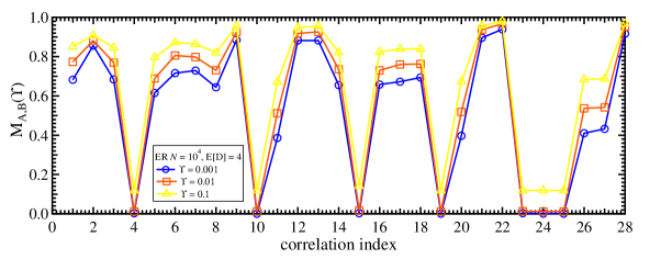
(a)

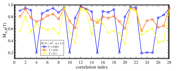
(b)

Figure 2: Centrality similarities between centrality metrics in network models: (a) for ER networks and (b) for SF networks. The x-axis is the correlation index (see Appendix B).

We observe that in both ER and SF networks, the $M_{B_{n},D}(\Upsilon)$ is notably larger than the centrality similarity between $B_{n}$ and any other centrality metric; $M_{C_{n},D^{(1)}}(\Upsilon)>M_{C_{n},D^{(2)}}(\Upsilon)>M_{C_{n},D}(\Upsilon)$; and the centrality similarities $M_{x_{1},D^{(1)}}(\Upsilon)$ and $M_{x_{1},D^{(2)}}(\Upsilon)$ are both large. In ER networks, $M_{x_{1},D^{(2)}}(\Upsilon)>M_{x_{1},D^{(1)}}(\Upsilon)>M_{x_{1},D}(\Upsilon)$. The $k$-shell index has low similarity with other metrics in ER networks for the same reason mentioned in Sec. 3.1. All these observations agree with what we have found using the Pearson correlation coefficients in Sec. 3.1.

3.2.2 Centrality similarities in real-world networks

For the 34 real-world networks the percentage $\Upsilon$ should be larger than 3%, since the smallest network only has 35 nodes. We compare the similarity between each centrality metric (e.g., $B_{n}$) and all other metrics to determine which metric is the closest to the centrality metric (e.g., $B_{n}$). In Fig. 3 the height of each bar indicates the number of networks in which $M_{A,B}(\Upsilon)$ is the highest among the centrality similarities between $A$ and all the other centrality metrics. The bar chart shows that the $D$, $D^{(1)}$, and $D^{(2)}$ are, respectively, most similar to $B_{n}$, $C_{n}$, and $x_{1}$ in most real-world networks, which is consistent with what is observed in the network models. We also observe that either $M_{L_{n},D}(\Upsilon)$ or $M_{L_{n},B_{n}}(\Upsilon)$ is the largest among the centrality similarities between $L_{n}$ and all other metrics in most real-world networks.

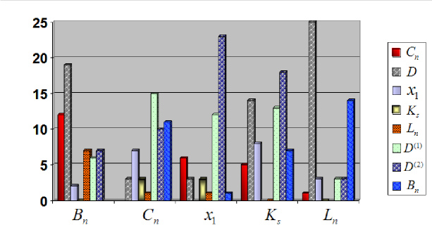
Figure 3: Number of networks (among the 34 real-world networks) in which $M_{A,B}(\Upsilon)$ is the highest among the centrality similarities between $A$ and all other centrality metrics, when $\Upsilon=5\%$. The centrality metric $A$ is given by the $x$-axis label, and $B$ is reflected by the pattern described in the box on right side. Take the betweenness $B_{n}$ as an example. The centrality similarities between $B_{n}$ and all the other metrics are compared with each other to find the largest similarity in each real-world network. For instance, the $M_{B_{n},C_{n}}(\Upsilon)$ is the largest centrality similarity in ‘Electric_s208’ network, so that one is counted into the leftmost bar of $B_{n}$ (with $C_{n}$).

4 Theoretical analysis

The above simulations indicate that the three lowest-order degree masses, with a low computational complexity, are strongly correlated with the betweenness, the closeness, and the components of the principal eigenvector, all of which are complex to compute. We first prove that the high-order ($m\rightarrow\infty$) degree mass is proportional to the principal eigenvector $x_{1}$ in any network. Next we prove that when $m$ is small the correlation between degree mass and the principal eigenvector increases with an increase in $m$, i.e., $\rho(X_{1},D^{(2)})\geq\rho(X_{1},D^{(1)})\geq\rho(X_{1},D)$. We then apply the generating function method [40, 41] to analyze such statistical properties of the degree masses as expectation and variance (see Appendix C).

Theorem 1

The $m$th-order degree mass vector $d^{(m)}$ is proportional to the principal eigenvector $x_{1}$ in any network with a sufficiently large spectral gap when $m\rightarrow\infty$.

Proof.

The $m$th-order degree mass vector $d^{(m)}$ is

$$d^{(m)} =\sum\limits_{k=1}^{m+1}\left(A^{k}u\right)={\displaystyle\sum\limits_{k=1}^{m+1}}{\displaystyle\sum\limits_{j=1}^{N}}\lambda_{j}^{k}x_{j}\left(x_{j}^{T}u\right)$$

$$={\displaystyle\sum\limits_{j=1}^{N}}\left(\lambda_{j}\frac{\lambda_{j}^{m+1}-1}{\lambda_{j}-1}\right)\left(x_{j}^{T}u\right)x_{j}$$

$$=\left(\lambda_{1}\frac{\lambda_{1}^{m+1}-1}{\lambda_{1}-1}\right)\left(x_{1}^{T}u\right)x_{1}+{\displaystyle\sum\limits_{j=2}^{N}}\left(\lambda_{j}\frac{\lambda_{j}^{m+1}-1}{\lambda_{j}-1}\right)\left(x_{j}^{T}u\right)x_{j}$$

$$=\left(\lambda_{1}\frac{\lambda_{1}^{m+1}-1}{\lambda_{1}-1}\right)\left(x_{1}^{T}u\right)x_{1}\left(1+O\left(\sum_{j=2}^{N}\left(\frac{\left|\lambda_{j}\right|}{\left|\lambda_{1}\right|}\right)^{m}\right)\right).$$

Literature [29] has proved that $x_{1}^{T}u>x_{j}^{T}u$ for all $1<j\leq N$. Accordingly, the term ${\displaystyle\sum\limits_{j=2}^{N}}\left(\lambda_{j}\frac{\lambda_{j}^{m+1}-1}{\lambda_{j}-1}\right)\left(x_{j}^{T}u\right)x_{j}$ is small in the graphs with a large spectral gap $(\lambda_{1}-\lambda_{2})$. When $m$ increases, $d^{(m)}\rightarrow\left(\lambda_{1}\frac{\lambda_{1}^{m+1}-1}{\lambda_{1}-1}\right)\left(x_{1}^{T}u\right)x_{1}$. Moreover, when $m$ is large, especially when $m\rightarrow\infty$, $O\left(\sum_{j=2}^{N}\left(\frac{\left|\lambda_{j}\right|}{\left|\lambda_{1}\right|}\right)^{m}\right)\rightarrow 0$ in any graph. Thus we find that $d^{(m)}$ tends to be proportional to $x_{1}$ when $m$ increases in networks with a large spectral gap, and $d^{(m)}\sim\lambda_{1}^{(m+1)}(x_{1})$ in networks when $m\rightarrow\infty$.   

Lemma 2

In large sparse Erdős-Rényi (ER) networks, $\rho(D^{(2)},X_{1})\geq\rho(D^{(1)},X_{1})\geq\rho(D,X_{1})$.

Proof. see Appendix C.   

5 Application to the inflexible contrarian opinion (ICO) model

In this section we apply the studied centrality metrics to select the inflexible contrarians in the inflexible contrarian opinion (ICO) model [27] to help one opinion to compete with another. Both network models and three social networks will be considered.

5.1 The ICO model

The ICO model is a variant of the non-consensus opinion (NCO) model [24]. The ICO and NCO models are both opinion competition models in which two opinions exist and compete with each other. In the NCO model opinions are randomly assigned to all agents (nodes). At time $t=0$ each agent is assigned opinion $A$ with a probability $f$ and opinion $B$ with a probability $1-f$. At each subsequent time step each agent adopts the opinion of the majority of its nearest neighbors and itself. When there is a tie, the opinion of the agent does not change. All of the updates are made simultaneously in parallel at each step. The system reaches a state in which the opinions $A$ and $B$ coexist and are stable when $f$ is above a critical threshold $f_{c}$.

When the NCO model is in the stable state, the ICO model further selects a fraction $p_{o}$ of agents with opinion $A$ to be the inflexible contrarians who will hold opinion $B$, will never change their opinion, but will influence the opinion of other agents. The two opinions then compete with each other according to the update rules of the NCO model. The system will reach a new stable state by following these opinion dynamics.

We use $S_{1}$ and $S_{2}$ to denote the size of the largest and the second largest clusters of agents with opinion $A$ in the new stable state. A phase transition threshold $f_{c}$ separates two different phases of the stable state. When $f>f_{c}$, a giant component of agents with opinion $A$ exists and the coexistence of opinions $A$ and $B$ is stable. When $f\leq f_{c}$, no giant component of agents with opinion $A$ exists ($S_{1}=0$). The $f_{c}$ depends on $p_{o}$. When $p_{o}=0$, the ICO model clearly reduces to the classical NCO model and they have the same critical threshold $f_{c}$. When $0<p_{o}<p^{\ast}$, the threshold $f_{c}$ of the ICO model increases with $p_{o}$, but the size $S_{1}$ for the finial stable state decreases with $p_{o}$. When $p$ is above a certain value $p^{\ast}$, the phase transition no longer occurs, and the giant component of agents with opinion $A$ is completely destroyed ($S_{1}=0$).

5.2 Strategies of selecting inflexible contrarians using centrality metrics

The final stable state of the ICO model is affected not only by the percentage $p_{o}$, but also by how inflexible contrarian agents are selected. Here we select the inflexible contrarians based on their centrality metrics. Li et al. [27] studied the ICO model by choosing the inflexible contrarian agents with opinion $A$ either randomly or according to highest degree. The degree strategy is significantly more effective than the random strategy in reducing the size $S_{1}$ of the largest opinion $A$ cluster in the stable state when $p_{o}$ is the same. Here we want to determine which centrality metric used to pick the inflexible contrarians reduces $S_{1}$ most efficiently. We also want to determine whether the $S_{1}$ decrease is similar when the inflexible contrarians are chosen based on two strongly correlated (with a large Pearson correlation coefficient or a high centrality similarity) centrality metrics. Here the inflexible contrarians are chosen as nodes with highest (i) betweenness, (ii) degree, (iii) $1$st-order degree mass, (iv) $2$nd-order degree mass, (v) eigenvector component, (vi) $k$-shell index, or (vii) leverage or (viii) chosen randomly.

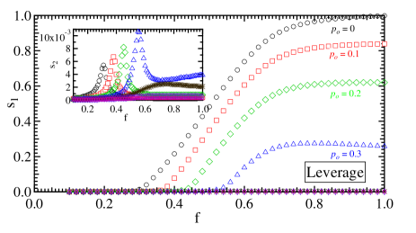
Figure 4: An example: the results of leverage strategy. Plot of $s_{1}\equiv S_{1}/N$ as a function of $f$ for different values of $p_{o}$ for ER networks with $E[D]=4$ and $N=10^{4}$. We denote by $S_{1}$ the size of the largest $A$ opinion cluster in the steady-state. Different marks show the results of ICO model with different $p_{o}$: $p_{o}$=0($\circ$), $p_{o}$=0.1($\square$), $p_{o}$=0.2($\diamond$), $p_{o}$=0.3($\triangle$), $p_{o}$=0.4($\ast$), $p_{o}$=0.5($\lozenge$), $p_{o}$=0.6($\boxtimes$). The insets plot the $s_{2}\equiv S_{2}/N$, where $S_{2}$ is the size of the second largest $A$ opinion cluster, as a function of the $f$ for different values of $p_{o}$.

5.3 Comparison of inflexible contrarian selection strategies

We first compare the efficiency in decreasing the size $S_{1}$ of the largest opinion $A$ cluster in ER and SF networks when choosing the inflexible contrarians using different centrality metrics. We consider ER networks ($N=10^{4}$ or $10^{5}$) with $E[D]=4$, and SF networks ($N=10^{4}$ or $10^{5}$) with $\alpha=2.5$, and perform all the simulations on $10^{3}$ network realizations. Figure 4 shows a plot of $s_{1}=S_{1}/N$ as a function of $f$ for different values of $p_{o}$ in ER networks (with $N=10^{4}$) using a leverage strategy. The size $s_{2}=S_{2}/N$ shows a sharp peak, a characteristic of a second-order phase transition, in the insets of Fig. 4. As $p_{o}$ increases, $f_{c}$ shifts to a larger value and the largest cluster becomes significantly smaller. When $p>p^{\ast}$, the giant component with opinion $A$ disappears, i.e., $S_{1}=0$. For example, the $p^{\ast}$ value for the leverage strategy is between 0.3 and 0.4 (see Fig. 4). A small $p^{\ast}$ implies that the inflexible contrarians can efficiently destroy the largest opinion $A$ cluster. We can compare the efficiency of the strategies in decreasing $S_{1}$ by the value of $p^{\ast}$. When we compare strategies in the ICO model with the same $p_{o}$, a larger phase transition $f_{c}$ for a strategy indicates that the inflexible contrarians chosen using this strategy decreases $S_{1}$ more efficiently. Figure 5a plots the phase transition $f_{c}$ as a function of $p_{o}$. Note that the efficiency of each strategy is ranked in decreasing order as: Leverage, Degree, Betweenness, $1$st-order Degree mass, $2$nd-order Degree mass, $k$-shell index, Principal Eigenvector, and Random. The same result can be also found in ER and SF networks with $N=10^{5}$.

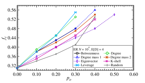
(a)

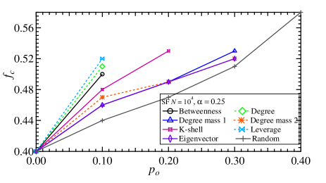
(b)

Figure 5: Plot of $f_{c}$ as a function of $p_{o}$ for strategies $1$ to $8$: (a) in ER graphs with $N=10^{4}$, $E[D]=4$; (b) in SF graphs with $N=10^{4}$, $D_{\min}=2$, $\alpha=2.5$.

We find that all strategies are more efficient in SF networks than in ER networks of the same size. We base this on two observations. First, the relative change of $f_{c}$ with $p_{o}$ for all strategies in SF networks is larger than it is in ER networks. Second, the $p^{\ast}$ for all strategies in SF is much smaller than it is in ER networks. The reason for this may be that (i) hubs can be readily selected as inflexible contrarians when using centrality metrics in SF networks, and (ii) hubs can strongly influence the opinion of their large number of nearest neighbors.

Figure 6 compares these centrality metrics in real-world networks, i.e., the ConMat 95-99 network, the ConMat 95-03 network, and the Astro_Ph network. Note that the inflexible contrarians selected using the leverage $L_{n}$, the betweenness $B_{n}$, and the degree $D$ are the most efficient in helping opinion $B$ win the competition. The similar behaviors of the three strategies are supported by the large Pearson correlation coefficient $\rho(B_{n}$, $D)$ and the large centrality similarities $M_{B_{n},D}(\Upsilon)$, $M_{L_{n},D}(\Upsilon)$ and $M_{L_{n},B_{n}}(\Upsilon)$.

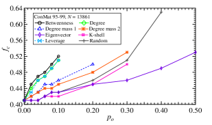
(a)

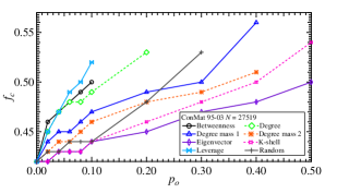
(b)

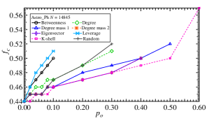
(c)

Figure 6: Plot of $f_{c}$ as a function of $p_{o}$ for strategies in social networks: (a) in network of coauthorships between scientists posting preprints on ConMat E-Print Archives between $1995$ to $1999$; (b) in network of coauthorships between scientists posting preprints on ConMat E-Print Archives between $1995$ to $2003$; (c) in network of coauthorships between scientists posting preprints on Astrophysics E-Print Archives between $1995$ to $1999$.

In both network models and real-world networks, strongly correlated centrality metrics tend to perform similarly. For example, we have discovered both numerically and theoretically that $\rho(D^{(2)},X_{1})\geq\rho(D^{(1)},X_{1})$. Correspondingly, the principal eigenvector $x_{1}$ strategy performs closer to the 2nd-order degree mass $D^{(2)}$ than the 1st-order degree mass $D^{(1)}$ in the ICO model.

6 Conclusion

In this paper we have studied the correlation between widely studied and recently proposed centrality metrics in numerous real-world networks as well as in network models, i.e., as in Erdős-Rényi (ER) random networks and scale-free (SF) networks. A strong correlation between two centrality metrics indicates the possibility of approximating one centrality metric, usually the one with a higher computational complexity, using the other. We study the correlations between the centrality metrics using the Pearson correlation coefficient and the centrality similarity. An important finding is that the degree $D$, the $1$st-order degree mass $D^{(1)}$, and the $2$nd-order degree mass $D^{(2)}$ are strongly correlated with the betweenness $B_{n}$, the closeness $C_{n}$, and the principal eigenvector $x_{1}$, respectively. This observation is partially supported by our analytical proof that $\rho(X_{1},D^{(2)})>\rho(X_{1},D^{(1)})>\rho(X_{1},D)$.

We have introduced the degree mass $D^{(m)}$ as a new network centrality metric. The $0$th-order degree mass is the degree and the high-order ($m\rightarrow\infty$) degree mass is proportional to the principal eigenvector $x_{1}$. We also find that the influence of network size (the number $N$ of nodes) on the Pearson correlation coefficients is small. In addition, the leverage $L_{n}$ has high centrality similarities with the degree $D$ and the betweenness $B_{n}$. We use these centrality metrics to select the inflexible contrarians in the ICO model to help one opinion to compete with the other. The leverage $L_{n}$ turns out to be the most efficient strategy in both network models and real-world networks. We also find that strongly correlated metrics perform similarly in the ICO model. This suggests that the metrics with a low computational complexity, such as the degree $D$ and the leverage $L_{n}$, could be used to approximate more complex metrics, e.g., the betweenness $B_{n}$, to locate important nodes in complex networks. Examples of important nodes would include inflexible contrarians in opinion propagation networks and nodes that should be immunized in disease transmission networks.

Acknowledgements

The authors are grateful to Shlomo Havlin for discussion and useful comments. This work has been supported by the European Commission within the framework of the CONGAS project FP7-ICT-2011-8-317672 and the China Scholarship Council (CSC).

Appendix A Description of the real-world networks

A.1 Descriptions

Table 1: Descriptions of real-world networks.

Index	Networks	Descriptions
1	American airline	The direct airport-to-airport American mileage a maintained by the U.S. Bureau of Transportation Statistics.
2	American football	This is the network of American football games between Division IA colleges during regular season Fall 2000, as compiled by M. Girvan and M. Newman.
3	ARPANET80	The Advanced Research Projects Agency Network as seen in 1980.
4	Celegensneural	Network representing the neural network of C. Elegans.
5	Dophins	An undirected social network of frequent associations between 62 dolphins in a community living off Doubtful Sound, New Zealand.
6	Dutch soccer	Dutch football players represent the nodes. Two nodes are linked if they played together a match.
7	Gnutella 1	Gnutella snapshots. Four different crawls are available.
8	Gnutella 2
9	Gnutella 3
10	Gnutella 4
11	Karate	Social network of friendships between 35 members of a karate club at a US university in the 1970.
12	LesMis	Coappearance network of characters in the novel Les Miserables.
13	Surfnet	SURFNET topology inferred from the switch interface interconnections.
14	Electric s208	ISCAS89 Sequential Benchmark Circuits. Each node represents a logical operation implemented
15	Electric s420	physically. Links between them relate their inputs/outputs.
16	Electric s838
17	Epowergridl1	Power-grid infrastructure at three different levels of one city-area in Western Europe.
18	Epowergridl2
19	Epowergridl3
20	Erailwayl1	Railway infrastructure at two levels of one Western-European country
21	Erailwayl2
22	WordAdj	Adjacency network of common adjectives and nouns in the novel David Copperfield by Charles Dickens.
23	WordAdjEnglish	Word-adjacency networks of texts in English, French and Japanese separately.
24	WordAdjFranch
25	WordAdjJapanese
26	Internet AS (01’)	Internet snapshot retrieved from the merge of different data sources (BGP routing tables and updates: Route Views, RIPE, Abilene, CERNET, BGP View).
27	Astro_Ph	Network of coauthorships between scientists posting preprints on the Astrophysics E-Print Archive between Jan 1, 1995 and December 31, 1999.
28	SciMet	Web of Science C. The citation network was created using the Web of Science database SciMet. Networks created with the tool HistCite.
29	HighE-th	High Energy Theory C. Network of coauthorships between scientists posting preprints on the High-Energy Theory E-Print Archive between Jan 1, 1995 and December 31, 1999.
30	CondMat 95-03	Network of coauthorships between scientists posting preprints on the Condensed Matter E-Print
31	CondMat 95-99	Archive. We have two networks corresponding to different periods of time. Periods are Jan 1, 1995-December 31, 1999 and 2003 respectively.
32	Dutch Roadmap	A graph representing the interconnection between cities in the Netherlands.
33	Network Science C	Coauthorship network of scientists working on network theory and experiment, as compiled by M. Newman in May 2006.
34	Next Generation	A typical Next Generation Transport network.

A.2 Properties of the real-world networks

The properties of real-world networks are shown in the Table 2. The definition of these properties has been described in detail in [42].

Table 2: Properties of real-world networks. The real-world network index is shown in Table 1. $N$ is the number of nodes, $L$ is the number of links. $E[H]$ is the average shortest path, $C_{G}$ is the clustering coefficient of networks. $\rho_{D}$ is the degree correlation coefficient (called the assortativity) of networks. $\lambda_{1}$ is the largest eigenvalue (called spectral radius) of the adjacency matrix of the network. $\mu_{N-1}$ is the second smallest Laplace eigenvalue (called spectral radius) of the networks. $\mu_{1}/\mu_{N-1}$ is the ratio of the largest eigenvalue $\mu_{1}$ and the second smallest eigenvalue $\mu_{1}$ of Laplacian matrix. $R_{G}$ is the effective graph resistance.

$\begin{array}[c]{|ccccccccccccc|}\hline\cr\hline\cr\text{Index}&N&L&E[H]&C_{G}&\rho_{D}&\lambda_{1}&\mu_{N-1}&\mu_{1}/\mu_{N-1}&R_{G}&E[D]&\sqrt{Var[D]}&H_{\max}\\ \hline\cr 1&2179&31326&3.0262&0.4849&-0.0409&144.6112&0.2082&2.0675e^{3}&1.6072e^{4}&28.7526&56.6782&8\\ 2&115&613&2.5082&0.4032&0.1624&10.7806&1.4590&10.7350&1.5086e^{3}&10.6609&0.8835&4\\ 3&71&86&6.4849&0.0141&-0.2613&2.7648&0.0374&170.2063&7.0158e^{3}&2.4225&0.7442&17\\ 4&297&2148&2.4553&0.2924&-0.1632&24.3655&0.8485&159.1562&1.3710e^{4}&14.4646&12.9443&5\\ 5&62&159&3.3570&0.2590&-0.0436&7.1936&0.1730&78.7034&1.8643e^{3}&5.1290&2.9319&8\\ 6&685&10310&4.4583&0.7506&-0.0634&50.8428&0.1613&372.0373&3.1157e^{4}&30.1022&21.1957&11\\ 7&737&803&9.1351&0.0063&-0.1934&4.8913&0.0073&2.6292e^{3}&1.4181e^{6}&2.1791&2.0069&24\\ 8&1568&1906&6.1037&0.0192&-0.0946&13.7828&0.0167&1.1205e^{4}&4.0212e^{4}&2.4311&5.5778&21\\ 9&435&459&6.7085&0.0145&-0.3301&8.2281&0.0110&5.9278e^{3}&4.2533e^{5}&2.1103&5.1534&20\\ 10&653&738&5.4513&0.0232&-0.2459&12.1145&0.0231&6.2319e^{3}&6.6603e^{5}&2.2603&7.0228&15\\ 11&35&134&1.9126&0.3908&-0.5036&9.6253&1.7264&12.6030&221.6283&7.6571&4.7265&3\\ 12&77&254&2.6411&0.5731&-0.1652&12.0058&0.2050&180.9490&3.0166e^{3}&6.5974&6.0006&5\\ 13&65&111&4.1236&0.0359&0.2288&5.0523&0.1137&92.7068&3.2979e^{3}&3.4154&1.9046&10\\ 14&122&189&4.9278&0.0591&-0.0020&4.1036&0.0836&135.2786&1.3082e^{4}&3.0984&1.4395&11\\ 15&252&399&5.8064&0.0651&-0.0059&4.3600&0.0512&297.3970&5.8313e^{4}&3.1667&1.5340&13\\ 16&512&819&6.8585&0.0547&-0.0300&5.0097&0.0285&809.9553&2.5149e^{5}&3.1992&1.6296&15\\ 17&3419&3953&21.1147&0.0120&-0.1283&5.1781&<e^{-5}&>e^{15}&4.8953e^{7}&2.3124&1.8425&51\\ 18&1205&1384&12.3547&0.0171&0.1082&4.8994&0.0022&9.1191e^{3}&4.3901e^{6}&2.2971&1.3609&31\\ 19&395&441&13.6088&0.0201&-0.0235&4.4854&0.0020&8.8844e^{3}&7.2535e^{5}&2.2329&1.2834&42\\ 20&8710&11332&79.0448&0.0212&-0.0219&2.9865&<e^{-5}&>e^{15}&7.2107e^{8}&2.6021&0.7696&213\\ 21&689&778&34.1261&0.0731&0.0980&3.6926&7.7321e^{-3}&1.0526e^{4}&3.9229e^{6}&2.2583&0.7658&84\\ 22&112&425&2.5356&0.1728&-0.1293&13.1502&0.6950&72.0767&3.7941e^{3}&7.5893&6.8512&5\\ 23&7377&44205&2.7780&0.4085&-0.2366&109.4416&<e^{-5}&9.1266e^{15}&2.2149e^{7}&11.9846&60.8260&8\\ 24&8308&23832&3.2189&0.2138&-0.2330&60.6735&0.1197&1.5810e^{4}&3.9917e^{7}&5.7371&34.8979&9\\ 25&2698&7995&3.0771&0.2196&-0.2590&42.9980&<e^{-5}&5.8851e^{15}&4.3489e^{6}&5.9266&24.6695&8\\ 26&12254&25319&3.6214&0.2992&-0.1903&61.1066&<e^{-5}&4.8974e^{15}&1.0349e^{8}&4.1324&33.5463&11\\ 27&14845&119652&4.7980&0.6696&0.2277&73.8868&0.0302&1.1966e^{4}&7.2012e^{7}&16.1202&21.7466&14\\ 28&2678&10368&4.1797&0.1736&-0.0352&20.4290&0.0853&1.9365e^{3}&2.9549e^{6}&7.7431&9.2480&12\\ 29&5835&13815&7.0264&0.5062&0.1852&18.0442&0.0214&2.3870e^{3}&2.8800e^{7}&4.7352&4.5571&19\\ 30&27519&116181&5.7667&0.6546&0.1657&40.3097&0.0276&7.3675e^{3}&3.3638e^{8}&8.4437&10.8110&16\\ 31&13861&44619&6.6278&0.6514&0.1571&24.9822&0.0292&3.6992e^{3}&1.1613e^{8}&6.4381&6.7598&18\\ 32&29663&34982&148.7102&0.0443&0.2462&3.4567&<e^{-5}&>e^{15}&1.5472e^{10}&2.3586&0.6823&531\\ 33&379&914&6.0419&0.7412&-0.0817&10.3755&0.0152&2.3053e^{3}&1.4826e^{5}&4.8232&3.9272&17\\ 34&29902&32707&7109.8681&0.0306&-0.0355&49.5455&<e^{-5}&>e^{15}&2.1188e^{12}&2.1876&9.7574&14253\\ \hline\cr\hline\cr\end{array}$

Appendix B Pearson correlation coefficients between centrality metrics

The correlation indexes mentioned in the following images and tables are the indexes for pairs of centrality metrics: $1$. $(B_{n},C_{n})$; $2$. $(B_{n},D)$; $3$. $(B_{n},x_{1})$; $4$. $(B_{n},K_{s})$; $5$. $(B_{n},L_{n})$; $6$. $(B_{n},D^{(1)})$; $7$. $(B_{n},D^{(2)})$; $8$. $(C_{n},D)$; $9$. $(C_{n},x_{1})$; $10$. $(C_{n},K_{s})$; $11$. $(C_{n},L_{n})$; $12$. $(C_{n},D^{(1)})$; $13$. $(C_{n},D^{(2)})$; $14$. $(D,x_{1})$; $15$. $(D,K_{s})$; $16$. $(D,L_{n})$; $17$. $(D,D^{(1)})$; $18$. $(D,D^{(2)})$; $19$. $(x_{1},K_{s})$; $20$. $(x_{1},L_{n})$; $21$. $(x_{1},D^{(1)})$; $22$. $(x_{1},D^{(2)})$; $23$. $(K_{s},L_{n})$; $24$. $(K_{s},D^{(1)})$; $25$. $(K_{s},D^{(2)})$; $26$. $(L_{n},D^{(1)})$; $27$. $(L_{n},D^{(2)})$; $28$. $(D^{(1)},D^{(2)})$.

Table 3: Pearson correlation coefficients among the centrality metrics in the real-world networks.

$\begin{array}[c]{|cccccccccc|}\hline\cr\hline\cr\text{Index}&1&2&3&4&5&6&7&8&9\\ &\rho(B_{n},C_{n})&\rho(B_{n},D)&\rho(B_{n},x_{1})&\rho(B_{n},K_{s})&\rho(B_{n},L_{n})&\rho(B_{n},D^{(1)})&\rho(B_{n},D^{(2)})&\rho(C_{n},D)&\rho(C_{n},x_{1})\\ \hline\cr 1&0.3667&0.5690&0.4119&0.3377&0.4027&0.4314&0.4224&0.7580&0.7684\\ 2&0.8167&0.2813&0.1450&0.0871&0.3212&0.2230&0.2075&0.2913&0.2462\\ 3&0.7129&0.7235&0.5358&0.3496&0.55585&0.7660&0.7593&0.4308&0.6851\\ 4&0.4271&0.7805&0.5206&0.1822&0.4212&0.5388&0.6044&0.6997&0.7827\\ 5&0.6657&0.5902&0.2835&0.4703&0.5639&0.5131&0.4850&0.7127&0.6979\\ 6&0.3303&0.4909&0.0857&0.1523&0.4170&0.3807&0.3113&0.2701&-0.1604\\ 7&0.4456&0.7292&0.4780&0.5182&0.4556&0.7575&0.7882&0.3973&0.5241\\ 8&0.2196&0.9691&0.7006&0.2677&0.2679&0.3858&0.9416&0.2225&0.5469\\ 9&0.2475&0.8839&0.4926&0.4667&0.4356&0.3533&0.8283&0.1763&0.5112\\ 10&0.2338&0.9603&0.5848&0.3296&0.3880&0.2640&0.8839&0.1774&0.5733\\ 11&0.8699&0.9651&0.8757&0.3782&0.8707&0.7999&0.9166&0.8853&0.9599\\ 12&0.6287&0.7468&0.4231&0.2388&0.5317&0.5534&0.5468&0.7997&0.6812\\ 13&0.7136&0.8743&0.7365&0.6345&0.6985&0.7999&0.7816&0.8290&0.9286\\ 14&0.6408&0.7475&0.5595&0.2147&0.5551&0.7357&0.7227&0.6127&0.7987\\ 15&0.5956&0.6933&0.5514&0.1583&0.4508&0.7084&0.7203&0.5541&0.7178\\ 16&0.5323&0.7044&0.5410&0.1314&0.3913&0.6971&0.7661&0.4623&0.5633\\ 17&0.2349&0.3843&0.1180&0.1189&0.1889&0.4101&0.4082&0.1082&0.0607\\ 18&0.3210&0.7005&0.5517&0.0560&0.2686&0.6772&0.7144&0.2946&0.4627\\ 19&0.3001&0.7081&0.4775&0.1060&0.2945&0.6371&0.6825&0.2395&0.4925\\ 20&0.2664&0.1565&-0.0442&0.1979&0.1112&0.1805&0.1876&0.1477&0.0209\\ 21&0.5022&0.3274&0.0364&0.3836&0.2548&0.2790&0.2540&0.2428&0.1141\\ 22&0.6559&0.9150&0.8226&0.3517&0.6586&0.7891&0.8444&0.8410&0.9245\\ 23&0.1880&0.9225&0.6525&0.2068&0.2642&0.4157&0.7765&0.3535&0.6528\\ 24&0.1874&0.9714&0.8047&0.2729&0.2636&0.4403&0.9385&0.2625&0.6215\\ 25&0.2747&0.9660&0.7859&0.3249&0.3584&0.5266&0.8972&0.3868&0.6880\\ 26&0.1382&0.9826&0.7994&0.3292&0.2290&0.3441&0.9582&0.1631&0.5776\\ 27&0.3764&0.6787&0.4353&0.2869&0.4631&0.5670&0.5270&0.6109&0.4220\\ 28&0.4068&0.8185&0.6959&0.3147&0.4401&0.7143&0.7605&0.6741&0.7030\\ 29&0.4526&0.7798&-0.0109&0.3574&0.5079&0.6700&0.5803&0.5774&0.0119\\ 30&0.3801&0.7534&0.3753&0.3152&0.4488&0.5933&0.5173&0.5989&0.3906\\ 31&0.4002&0.7225&0.2781&0.2607&0.4581&0.5718&0.4816&0.5616&0.3248\\ 32&0.2214&0.1741&-0.0037&0.1619&0.1117&0.1719&0.1608&0.1450&-0.0221\\ 33&0.4302&0.6883&0.1884&0.1917&0.4707&0.5630&0.4997&0.3468&0.2593\\ 34&-0.1342&-0.0436&-0.6295&-0.9718&0.9538&-0.9051&-0.1342&0.0313&0.2446\\ \hline\cr\hline\cr\end{array}$

$\begin{array}[c]{|ccccccccccc|}\hline\cr\hline\cr\text{Index}&10&11&12&13&14&15&16&17&18&19\\ &\rho(C_{n},K_{s})&\rho(C_{n},L_{n})&\rho(C_{n},D^{(1)})&\rho(C_{n},D^{(2)})&\rho(D,x_{1})&\rho(D,K_{s})&\rho(D,L_{n})&\rho(D,D^{(1)})&\rho(D,D^{(2)})&\rho(x_{1},K_{s})\\ \hline\cr 1&0.8174&0.5944&0.7903&0.7712&0.9592&0.8730&0.7259&0.9657&0.9643&0.9254\\ 2&0.1742&0.2704&0.2826&0.2839&0.7501&0.3881&0.9181&0.9619&0.9314&0.2456\\ 3&0.3807&0.2524&0.5598&0.5870&0.4650&0.5127&0.8914&0.9020&0.9079&0.1326\\ 4&0.6861&0.5776&0.8680&0.7951&0.7810&0.5434&0.7886&0.8830&0.9311&0.5572\\ 5&0.7498&0.6094&0.7475&0.7422&0.7196&0.8303&0.9050&0.9574&0.9417&0.5388\\ 6&0.0680&0.2221&0.2381&0.1801&0.6237&0.7300&0.8963&0.9393&0.8801&0.7983\\ 7&0.5073&0.2052&0.6184&0.6248&0.4660&0.5933&0.8117&0.8217&0.8573&0.3912\\ 8&0.4015&0.0017&0.7515&0.3210&0.6523&0.3463&0.3888&0.3594&0.9132&0.1840\\ 9&0.2377&-0.3534&0.8326&0.3544&0.5811&0.3316&0.4651&0.3050&0.9493&0.2032\\ 10&0.2234&-0.2234&0.8594&0.2967&0.6366&0.2492&0.3751&0.2256&0.9481&0.0868\\ 11&0.5492&0.7227&0.9606&0.9463&0.9392&0.5331&0.9390&0.8718&0.9714&0.6221\\ 12&0.5622&0.6340&0.8375&0.7931&0.8467&0.7969&0.8474&0.9455&0.9380&0.8100\\ 13&0.7311&0.3466&0.9330&0.9363&0.9046&0.8289&0.7598&0.9486&0.9391&0.8425\\ 14&0.5670&0.3265&0.7388&0.7574&0.6757&0.4296&0.8184&0.9260&0.9225&0.3108\\ 15&0.5257&0.2675&0.6964&0.7100&0.6147&0.3995&0.7980&0.9078&0.9200&0.2464\\ 16&0.4949&0.1937&0.6534&0.6411&0.4120&0.3738&0.7690&0.8670&0.9055&0.1143\\ 17&-0.0402&-0.0122&0.1651&0.1653&0.2143&0.4102&0.6878&0.7733&0.8456&0.0447\\ 18&0.1582&0.1027&0.4752&0.4902&0.5040&0.1904&0.5901&0.8725&0.8851&0.0638\\ 19&0.2490&0.2137&0.5599&0.5316&0.5183&0.2287&0.5911&0.7611&0.8338&0.0327\\ 20&0.1649&0.0836&0.1829&0.2016&0.1031&0.7905&0.9247&0.9522&0.9241&0.1132\\ 21&0.4880&0.0325&0.3314&0.3382&0.2678&0.4149&0.7508&0.8884&0.8524&0.0835\\ 22&0.8194&0.7371&0.9451&0.9123&0.9575&0.6433&0.8327&0.9390&0.9707&0.7010\\ 23&0.7195&0.3891&0.8312&0.5353&0.8704&0.4649&0.4862&0.6580&0.9504&0.7992\\ 24&0.6355&0.0669&0.8167&0.4111&0.8733&0.4146&0.3627&0.5403&0.9779&0.6980\\ 25&0.6814&0.2080&0.8410&0.5506&0.8911&0.5155&0.5048&0.6631&0.9694&0.7628\\ 26&0.4291&-0.0707&0.7971&0.2788&0.8253&0.3935&0.2696&0.3771&0.9754&0.5413\\ 27&0.5427&0.2819&0.5861&0.5264&0.7188&0.8070&0.5920&0.9352&0.8728&0.5695\\ 28&0.8188&0.5093&0.7923&0.7456&0.8345&0.6962&0.7237&0.9204&0.9236&0.6212\\ 29&0.4884&0.2103&0.6517&0.6022&0.1789&0.7311&0.7080&0.9080&0.8292&0.5171\\ 30&0.6341&0.2404&0.6153&0.5392&0.6346&0.7339&0.6197&0.9035&0.8259&0.5001\\ 31&0.5157&0.2077&0.6067&0.5300&0.5304&0.7166&0.6631&0.8941&0.8021&0.4229\\ 32&0.1465&-0.0170&0.2033&0.2220&0.0364&0.5291&0.7674&0.9271&0.8880&0.0101\\ 33&0.0926&0.0970&0.4562&0.4120&0.4748&0.6803&0.7723&0.8795&0.8415&0.4195\\ 34&0.3609&-0.3531&0.3378&0.0649&0.7297&0.0866&0.0487&0.1570&0.9858&0.6768\\ \hline\cr\hline\cr\end{array}$

$\begin{array}[c]{|cccccccccc|}\hline\cr\hline\cr\text{Index}&20&21&22&23&24&25&26&27&28\\ &\rho(x_{1},L_{n})&\rho(x_{1},D^{(1)})&\rho(x_{1},D^{(2)})&\rho(K_{s},L_{n})&\rho(K_{s},D^{(1)})&\rho(K_{s},D^{(2)})&\rho(L_{n},D^{(1)})&\rho(L_{n},D^{(2)})&\rho(D^{(1)},D^{(2)})\\ \hline\cr 1&0.6327&0.9978&0.9998&0.7122&0.9389&0.9245&0.6604&0.6405&0.9984\\ 2&0.4881&0.8660&0.9134&0.4481&0.3467&0.3274&0.7771&0.7189&0.9929\\ 3&0.1934&0.6460&0.7101&0.5798&0.4773&0.4407&0.6485&0.6530&0.9811\\ 4&0.6130&0.9783&0.9885&0.7710&0.6277&0.5737&0.6605&0.6789&0.9813\\ 5&0.4991&0.8285&0.8842&0.8506&0.8171&0.7668&0.7887&0.7535&0.9913\\ 6&0.3684&0.8132&0.8867&0.6089&0.8563&0.8700&0.7478&0.6517&0.9864\\ 7&0.2262&0.6736&0.7412&0.4906&0.6480&0.5920&0.5024&0.4922&0.9475\\ 8&0&0.8135&0.8463&0.5030&0.3187&0.2061&-0.0050&0.1176&0.4936\\ 9&-0.1161&0.7007&0.7440&0.3782&0.2365&0.2762&-0.3636&0.2134&0.4889\\ 10&-0.1437&0.7414&0.8018&0.5184&0.1290&0.1398&-0.3598&0.1438&0.3751\\ 11&0.8128&0.9837&0.9930&0.5722&0.6484&0.5928&0.7290&0.8623&0.9568\\ 12&0.6520&0.9427&0.9691&0.7984&0.8524&0.8447&0.7713&0.7455&0.9924\\ 13&0.4673&0.9841&0.9927&0.6005&0.8604&0.8512&0.5510&0.5248&0.9969\\ 14&0.3310&0.8087&0.8589&0.2983&0.4885&0.4576&0.6007&0.5809&0.9839\\ 15&0.2497&0.7503&0.8010&0.2684&0.4523&0.4137&0.5520&0.5475&0.9788\\ 16&0.0562&0.5789&0.6656&0.2530&0.4262&0.3673&0.4862&0.4847&0.9533\\ 17&0.0545&0.3371&0.3805&0.7626&0.1513&0.1393&0.2283&0.2760&0.9458\\ 18&0.0501&0.6365&0.6794&0.3420&0.1429&0.1199&0.2204&0.2123&0.9812\\ 19&0.0748&0.7433&0.7697&0.3351&0.1335&0.1077&0.0448&0.1010&0.9619\\ 20&0.0564&0.1303&0.1454&0.6233&0.8541&0.8624&0.7665&0.7184&0.9907\\ 21&0.0347&0.4062&0.4780&0.2918&0.4205&0.3829&0.4013&0.3398&0.9842\\ 22&0.7490&0.9949&0.9983&0.8031&0.7300&0.6910&0.7541&0.7622&0.9888\\ 23&0.6646&0.9320&0.9790&0.7406&0.8912&0.6890&0.6611&0.6156&0.8432\\ 24&0.3912&0.8774&0.9476&0.5641&0.7939&0.5488&0.3408&0.3734&0.6794\\ 25&0.5507&0.9242&0.9721&0.6990&0.8180&0.6646&0.4857&0.5386&0.8112\\ 26&0.1486&0.8169&0.8977&0.4876&0.5646&0.4417&0.0699&0.1943&0.4845\\ 27&0.2248&0.8789&0.9367&0.4761&0.7840&0.7124&0.3996&0.3245&0.9845\\ 28&0.4680&0.9417&0.9682&0.7181&0.7457&0.6886&0.5866&0.5501&0.9877\\ 29&0.0427&0.2885&0.3822&0.5164&0.7657&0.7361&0.4493&0.3477&0.9771\\ 30&0.1765&0.8431&0.9205&0.5016&0.7344&0.6617&0.3726&0.2850&0.9795\\ 31&0.1358&0.7641&0.8725&0.4877&0.7372&0.6597&0.3945&0.2903&0.9731\\ 32&0.0063&0.0524&0.0629&0.3943&0.5167&0.4740&0.4892&0.4156&0.9878\\ 33&0.1267&0.7062&0.8105&0.5701&0.7390&0.6966&0.5089&0.4324&0.9766\\ 34&-0.5920&0.7797&0.8022&-0.9766&0.9347&0.1797&-0.9156&-0.0611&0.2549\\ \hline\cr\hline\cr\end{array}$

Appendix C Proof of Lemmas

C.1

Lemma 3

In an Erdős-Rényi (ER) random network $G_{p}(N)$, when $N\rightarrow\infty$, the average $1$st-order degree mass is

$$E[D^{(1)}]=N(2p+p^{2}N)\text{,}$$ (1)

and the variance is

$$Var[D^{(1)}]=N(2p+4p^{2}N+p^{3}N^{2})\text{.}$$ (2)

The average and the variance of $2$nd-order degree mass are

$$E[D^{(2)}]=N(2p+3p^{2}N+p^{3}N^{2})\text{,}$$ (3)

$$Var[D^{(2)}]=N(2p+14p^{2}N+17p^{3}N^{2}+7p^{4}N^{3}+p^{5}N^{4})\text{.}$$ (4)

Proof. The generating function for the probability distribution of node degree is defined as

$$\varphi_{D}(z)=\sum_{k=0}^{N-1}z^{k}\mathrm{Prob}[D=k]\text{,}$$

and the generating function of the degree of the node that we arrive at by following a randomly chosen link is

$$\frac{\sum_{k}k\mathrm{Prob}[D=k]z^{k}}{\sum_{k}k\mathrm{Prob}[D=k]}=z\frac{\varphi_{D}^{\prime}(z)}{E[D]}\text{,}$$ (5)

where $E[.]$ is the expectation. If we start at a randomly chosen node, the generating function of the degree of a nearest neighbor of this node follows Eq. (5). The $1$st-order degree mass $D^{(1)}$ of a node equals the degree sum of the node and its neighbors. The generating function has the ‘powers’ property [41], that the distribution of the $1$st-order degree mass of a node obtained from one nearest neighbor is generated by

$$\varphi_{D}(z)^{\ast}=z^{2}\frac{\varphi_{D}^{\prime}(z)}{E[D]}\text{,}$$

then, the distribution of the total of the $1$st-order degree mass over $k$ independent realizations ($k$ nearest neighbors) of the node is generated by $k$th power of $\varphi_{D}(z)^{\ast}$ as

$$\varphi_{D^{(1)}}(z)=\varphi_{D}(\varphi_{D}(z)^{\ast})=\sum_{k}\mathrm{Prob}[D=k]\left(z^{2}\frac{\varphi_{D}^{\prime}(z)}{E[D]}\right)^{k}\text{.}$$ (6)

For ER networks, $E[D]=(N-1)p$ is the average degree in an ER network $G_{p}(N)$, and $\varphi_{D}(z)=(1-p+pz)^{N-1}$, thus,

$$\varphi_{D^{(1)}}(z)=((1-p)+z^{2}p(1-p+pz)^{N-2})^{N-1}\text{,}$$ (7)

In addition, the generating function has the ‘Moments’ property [41], that $E[\left(D^{(1)}\right)^{n}]=\left[(z\frac{d}{dz})^{n}\varphi_{D^{(1)}}(z)\right]_{z=1}$. Together with $Var[D^{(1)}]=E[\left(D^{(1)}\right)^{2}]-E[D^{(1)}]^{2}$, we arrive at the (1) and (2), when $N\rightarrow\infty$.

Similarly, the distribution of the $2$nd-order degree mass is generated by $\varphi_{D}(\varphi_{D^{(1)}}(\varphi_{D^{(1)}}(z)))$. Hence, we obtain the generating function of the $2$nd-order degree mass as

$$\varphi_{D^{(2)}}(z)=(1-p+pz^{2}(1-p+pz)^{N-2}(1-p+pz^{2}(1-p+pz)^{N-2})^{N-2})^{N-1}\text{,}$$

Thus, we can obtain (3) and (4).   

C.2 Proof of Lemma2

Proof. The eigenvalue equation $Ax=\lambda x$ leads to $\lambda_{1}^{k}x_{1}=A^{k}x_{1}$, from which we obtain $u^{T}x_{1}{\displaystyle\sum\limits_{j=1}^{m}}\lambda_{1}^{j}=u^{T}\left({\displaystyle\sum\limits_{j=1}^{m}}A^{j}\right)x_{1}\text{,}$ where $u^{T}x_{1}=NE[X_{1}]$ and $u^{T}{\displaystyle\sum\limits_{j=1}^{m+1}}A^{j}=\left(d^{(m)}\right)^{T}$. Hence, the relation between the principal eigenvector and the $m$th-order degree mass vector can be expressed as $E[X_{1}]N{\displaystyle\sum\limits_{j=1}^{m+1}}\lambda_{1}^{j}=\left(d^{(m)}\right)^{T}x_{1}$, leading to

$$E[D^{(m)}X_{1}]=E[X_{1}]{\displaystyle\sum\limits_{j=1}^{m+1}}\lambda_{1}^{j}.$$ (8)

The Pearson correlation coefficient follows as

$$\rho(D^{(m)},X_{1})=\frac{E[D^{(m)}X_{1}]-E[D^{(m)}]E[X_{1}]}{\sqrt{Var[D^{(m)}]}\sqrt{Var[X_{1}]}}=\frac{\left({\displaystyle\sum\limits_{j=1}^{m+1}}\lambda_{1}^{j}-E[D^{(m)}]\right)E[X_{1}]}{\sqrt{Var[D^{(m)}]}\sqrt{Var[X_{1}]}}\text{.}$$ (9)

The ratio of the two Pearson correlation coefficients is

$$\frac{\rho(D^{(1)},X_{1})}{\rho(D,X_{1})}=\frac{\sqrt{Var[D]}}{\sqrt{Var[D^{(1)}]}}\left(1+\frac{(\lambda_{1}^{2}-E[D^{2}])}{\left(\lambda_{1}-E[D]\right)}\right)$$ (10)

For large ER graphs, $E[D]=(N-1)p\rightarrow Np$, $E[D^{2}]=(N-1)^{2}p^{2}-(N-1)p^{2}+(N-1)p\rightarrow N^{2}p^{2}-Np^{2}+Np$ and $Var[D]=(N-1)p(1-p)\rightarrow Np(1-p)$. From (2), we obtain

$$\frac{\sqrt{Var[D]}}{\sqrt{Var[D^{(1)}]}}=\sqrt{\frac{(1-p)}{(E[D]+2)^{2}-2}}>\frac{1}{E[D]+2}\text{.}$$ (11)

When $N\rightarrow\infty$ and $Np=\varsigma$ ($\varsigma$ is a constant and independent of $N$), the spectral radius $\lambda_{1}\rightarrow\varsigma$, in sparse random graphs [43, 44]. With (10) and (11), $\rho(D^{(1)},X_{1})\geq\rho(D,X_{1})$ is proved.

The ratio of the two Pearson correlation coefficients is

$$\frac{\rho(D^{(2)},X_{1})}{\rho(D^{(1)},X_{1})}=\frac{\left(\lambda_{1}+\lambda_{1}^{2}+\lambda_{1}^{3}-E[D^{(2)}]\right)\sqrt{Var[D^{(1)}]}}{\left(\lambda_{1}+\lambda_{1}^{2}-E[D^{2}]-E[D]\right)\sqrt{Var[D^{(2)}]}}\text{,}$$

with (3) and $\lambda_{1}\rightarrow Np$, when $N\rightarrow\infty$ we arrive at

$$\frac{\left(\lambda_{1}+\lambda_{1}^{2}+\lambda_{1}^{3}-E[D^{(2)}]\right)}{\left(\lambda_{1}+\lambda_{1}^{2}-E[D^{2}]-E[D]\right)}=2E[D]+1\text{.}$$

With (2) and (4), for large sparse random networks, $\rho(D^{(2)},X_{1})\geq\rho(D^{(1)},X_{1})$ is proved.

References

• [1] S.Β H. Strogatz, β€œExploring complex networks,” Nature, vol.Β 410, no.Β 6825, pp.Β 268–276, 2001.
• [2] S.Β Boccaletti, V.Β Latora, Y.Β Moreno, M.Β Chavez, and D.-U. Hwang, β€œComplex networks: Structure and dynamics,” Physics reports, vol.Β 424, no.Β 4, pp.Β 175–308, 2006.
• [3] A.Β Barrat, M.Β Barthelemy, and A.Β Vespignani, Dynamical processes on complex networks. Cambridge University Press, Cambridge, U.K., 2008.
• [4] C.Β H. Comin and L.Β daΒ FontouraΒ Costa, β€œIdentifying the starting point of a spreading process in complex networks,” Physical Review E, vol.Β 84, no.Β 5, p.Β 056105, 2011.
• [5] M.Β Kitsak, L.Β K. Gallos, S.Β Havlin, F.Β Liljeros, L.Β Muchnik, H.Β E. Stanley, and H.Β A. Makse, β€œIdentification of influential spreaders in complex networks,” Nature Physics, vol.Β 6, no.Β 11, pp.Β 888–893, 2010.
• [6] J.Β Borge-Holthoefer and Y.Β Moreno, β€œAbsence of influential spreaders in rumor dynamics,” Physical Review E, vol.Β 85, no.Β 2, p.Β 026116, 2012.
• [7] R.Β Pastor-Satorras and A.Β Vespignani, β€œImmunization of complex networks,” Physical Review E, vol.Β 65, no.Β 3, p.Β 036104, 2002.
• [8] S.Β P. Borgatti, β€œCentrality and network flow,” Social networks, vol.Β 27, no.Β 1, pp.Β 55–71, 2005.
• [9] L.Β C. Freeman, β€œCentrality in social networks conceptual clarification,” Social networks, vol.Β 1, no.Β 3, pp.Β 215–239, 1979.
• [10] N.Β E. Friedkin, β€œTheoretical foundations for centrality measures,” American journal of Sociology, vol.Β 96, pp.Β 1478–1504, 1991.
• [11] B.Β Mullen, C.Β Johnson, and E.Β Salas, β€œEffects of communication network structure: Components of positional centrality,” Social Networks, vol.Β 13, no.Β 2, pp.Β 169–185, 1991.
• [12] M.Β E.Β J. Newman, β€œThe mathematics of networks,” The new palgrave encyclopedia of economics, vol.Β 2, pp.Β 1–12, 2008.
• [13] P.Β VanΒ Mieghem, β€œGraph eigenvectors, fundamental weights and centrality metrics for nodes in networks,” arXiv preprint arXiv:1401.4580, 2014.
• [14] K.Β E. Joyce, P.Β J. Laurienti, J.Β H. Burdette, and S.Β Hayasaka, β€œA new measure of centrality for brain networks,” PLoS One, vol.Β 5, no.Β 8, p.Β e12200, 2010.
• [15] P.-J. Kim and H.Β Jeong, β€œReliability of rank order in sampled networks,” The European Physical Journal B, vol.Β 55, no.Β 1, pp.Β 109–114, 2007.
• [16] D.Β KoschΓΌtzki and F.Β Schreiber, β€œComparison of centralities for biological networks,” in German Conference on Bioinformatics, pp.Β 199–206, 2004.
• [17] E.Β Estrada, β€œCharacterization of topological keystone species: local, global and meso-scale centralities in food webs,” Ecological Complexity, vol.Β 4, no.Β 1, pp.Β 48–57, 2007.
• [18] C.Β Li, H.Β Wang, and P.Β VanΒ Mieghem, β€œDegree and principal eigenvectors in complex networks,” in Proceedings of NETWORKING 2012, pp.Β 149–160, Springer, 2012.
• [19] P.Β ErdΕ‘s and A.Β RΓ©nyi, β€œOn random graphs, i.,” Publ. Math. Debrecen, vol.Β 6, pp.Β 290–297, 1959.
• [20] A.-L. BarabΓ‘si and R.Β Albert, β€œEmergence of scaling in random networks,” science, vol.Β 286, no.Β 5439, pp.Β 509–512, 1999.
• [21] R.Β Cohen and S.Β Havlin, Complex networks: structure, robustness and function. Cambridge University Press, Cambridge, U.K., 2010.
• [22] S.Β Galam, β€œLocal dynamics vs. social mechanisms: A unifying frame,” EPL (Europhysics Letters), vol.Β 70, no.Β 6, p.Β 705, 2005.
• [23] C.Β Castellano, S.Β Fortunato, and V.Β Loreto, β€œStatistical physics of social dynamics,” Reviews of modern physics, vol.Β 81, no.Β 2, p.Β 591, 2009.
• [24] J.Β Shao, S.Β Havlin, and H.Β E. Stanley, β€œDynamic opinion model and invasion percolation,” Physical review letters, vol.Β 103, no.Β 1, p.Β 018701, 2009.
• [25] Q.Β Li, L.Β A. Braunstein, H.Β Wang, J.Β Shao, H.Β E. Stanley, and S.Β Havlin, β€œNon-consensus opinion models on complex networks,” Journal of Statistical Physics, vol.Β 151, no.Β 1-2, pp.Β 92–112, 2013.
• [26] B.Β Qu, Q.Β Li, S.Β Havlin, H.Β E. Stanley, and H.Β Wang, β€œNon-consensus opinion model on directed networks,” arXiv preprint arXiv:1404.7318, 2014.
• [27] Q.Β Li, L.Β A. Braunstein, S.Β Havlin, and H.Β E. Stanley, β€œStrategy of competition between two groups based on an inflexible contrarian opinion model,” Physical Review E, vol.Β 84, no.Β 6, p.Β 066101, 2011.
• [28] P.Β VanΒ Mieghem, Performance Analysis of Complex Networks and Systems. Cambridge University Press, 2014.
• [29] P.Β VanΒ Mieghem, Graph spectra for complex networks. Cambridge University Press, Cambridge, U.K., 2011.
• [30] J.Β M. Anthonisse, β€œThe rush in a directed graph,” Stichting Mathematisch Centrum. Mathematische Besliskunde, no.Β BN 9/71, pp.Β 1–10, 1971.
• [31] H.Β Wang, J.Β M. Hernandez, and P.Β VanΒ Mieghem, β€œBetweenness centrality in a weighted network,” Physical Review E, vol.Β 77, no.Β 4, p.Β 046105, 2008.
• [32] D.Β KoschΓΌtzki, K.Β A. Lehmann, L.Β Peeters, S.Β Richter, D.Β Tenfelde-Podehl, and O.Β Zlotowski, β€œCentrality indices,” in Network analysis, pp.Β 16–61, Springer, 2005.
• [33] H.-W. Ma and A.-P. Zeng, β€œThe connectivity structure, giant strong component and centrality of metabolic networks,” Bioinformatics, vol.Β 19, no.Β 11, pp.Β 1423–1430, 2003.
• [34] S.Β B. Seidman, β€œNetwork structure and minimum degree,” Social networks, vol.Β 5, no.Β 3, pp.Β 269–287, 1983.
• [35] B.Β Pittel, J.Β Spencer, and N.Β Wormald, β€œSudden emergence of a giant k-core in a random graph,” Journal of Combinatorial Theory, Series B, vol.Β 67, no.Β 1, pp.Β 111–151, 1996.
• [36] V.Β Batagelj and M.Β Zaversnik, β€œAn o (m) algorithm for cores decomposition of networks,” arXiv preprint cs/0310049, 2003.
• [37] R.Β Cohen, K.Β Erez, D.Β Ben-Avraham, and S.Β Havlin, β€œResilience of the internet to random breakdowns,” Physical review letters, vol.Β 85, no.Β 21, p.Β 4626, 2000.
• [38] M.Β P. Joy, A.Β Brock, D.Β E. Ingber, and S.Β Huang, β€œHigh-betweenness proteins in the yeast protein interaction network,” BioMed Research International, vol.Β 2005, no.Β 2, pp.Β 96–103, 2005.
• [39] S.Β Trajanovski, J.Β MartΓ­n-HernΓ‘ndez, W.Β Winterbach, and P.Β VanΒ Mieghem, β€œRobustness envelopes of networks,” Journal of Complex Networks, vol.Β 1, no.Β 1, pp.Β 44–62, 2013.
• [40] P.Β VanΒ Mieghem, Performance analysis of communications networks and systems. Cambridge University Press, Cambridge, U.K., 2006.
• [41] M.Β E.Β J. Newman, S.Β H. Strogatz, and D.Β J. Watts, β€œRandom graphs with arbitrary degree distributions and their applications,” Physical Review E, vol.Β 64, no.Β 2, p.Β 026118, 2001.
• [42] C.Β Li, H.Β Wang, W.Β deΒ Haan, C.Β J. Stam, and P.Β VanΒ Mieghem, β€œThe correlation of metrics in complex networks with applications in functional brain networks,” Journal of Statistical Mechanics: Theory and Experiment, vol.Β 2011, no.Β 11, p.Β P11018, 2011.
• [43] M.Β Krivelevich and B.Β Sudakov, β€œThe largest eigenvalue of sparse random graphs,” Combinatorics, Probability and Computing, vol.Β 12, no.Β 1, pp.Β 61–72, 2003.
• [44] I.Β J. Farkas, I.Β DerΓ©nyi, A.-L. BarabΓ‘si, and T.Β Vicsek, β€œSpectra of real-world graphs: Beyond the semicircle law,” Physical Review E, vol.Β 64, no.Β 2, p.Β 026704, 2001.