Incompressible limit of mechanical model of tumor growth with viscosity

Abstract

Various models of tumor growth are available in the litterature. A first class describes the evolution of the cell number density when considered as a continuous visco-elastic material with growth. A second class, describes the tumor as a set and rules for the free boundary are given related to the classical Hele-Shaw model of fluid dynamics.

Following the lines of previous papers where the material is described by a purely elastic material, or when active cell motion is included, we make the link between the two levels of description considering the ‘stiff pressure law’ limit. Even though viscosity is a regularizing effect, new mathematical difficulties arise in the visco-elastic case because estimates on the pressure field are weaker and do not imply immediately compactness. For instance, traveling wave solutions and numerical simulations show that the pressure may be discontinous in space which is not the case for the elastic case.

Key-words: Tumor growth; Hele-Shaw equation; Free boundary problems; Porous media; Viscoelastic media
Mathematical Classification numbers: 35J60; 35K57; 74J30; 92C10;

1 The cell model with visco-elastic flow

We consider a mechanical model of tumor growth considered as a visco-elastic media. We denote the number density of tumor cells by $n(x,t)$, the pressure by $p(x,t)$ and we assume a Brinkman flow that means the macroscopic velocity field is given by $\nabla W$ for a potential $W$ closely related to the pressure. With these assumptions, the model for tumor growth writes

$$\displaystyle\partial_{t}n_{k}-{\rm div}(n_{k}\nabla W_{k})=n_{k}G\big{(}p_{k}\big{)},$$ (1)

$$\displaystyle-\nu\Delta W_{k}+W_{k}=p_{k}(x,t):=\Pi_{k}(n_{k}),$$ (2)

where we choose the pressure law given by:

$$\Pi_{k}(n)=\frac{k}{k-1}n^{k-1},\qquad k>2.$$ (3)

Following [8, 22], we assume that growth is directly related to the pressure through a function $G(\cdot)$ that satisfies

$$G\in C^{1}(\mathbb{R}),\qquad G^{\prime}(\cdot)\leq-\alpha<0,\qquad G(P_{M})=0\quad\text{ for some }\;P_{M}>0.$$ (4)

The pressure $P_{M}$ is usually called the homeostatic pressure . We complete equation (1), (2) with a family of initial data $n^{0}_{k}$ satisfying (for some constant $C$ independent of $k$)

$$0\leq n^{0}_{k},\qquad\Pi_{k}(n^{0}_{k})\leq p_{M},\qquad\|n^{0}_{k}\|_{L^{1}(\mathbb{R}^{d})}\leq C.$$ (5)

The viscosity coefficient, $\nu>0$, is supposed to be constant; when viscosity is neglected, that means equation (2) with $\nu=0$, we recover Darcy’s law for which an important literature is available, see [10, 24, 15, 23, 11, 16, 19, 18] and the references therein. In that case only friction with the cell surrounding (extra-cellular matrix) is considered. Viscosity is a way to represent friction between cells themselves, considered as a Newtonian fluid and Brinkman’s law has been derived rigorously for inhomogenous materials [2]. Viscoelastic models for tumor growth, based on Stokes’ or Brinkman’s law have also been used in the context of tumor growth is [26, 7, 22] with a major difference, namely the pressure does not follow a law-of-state (4) but follows from the tissue incompressibility. However, Stokes’ or Brinkman’s law are also used considering the tissue as ‘compressible’ [6, 4]. To use Laplacian in (2), rather than Stokes viscosity terms, is to simplify the presentation and presentation of the mathematical ideas. Indeed, this is not central for our aim here, which is to explain the derivation of such ‘incompressible’ models from the ‘compressible’ equations. Note that the theory of mixtures allows for a general formalism containing both Darcy’s law and Brinkman’s law [9, 3, 21].

Our interest is in the ‘stiff pressure law’ limit of this model towards a free boundary model which generalizes the classical Hele-Shaw equation. That is the limit $k\to\infty$ and we first explain formally what can be expected. The limit uses strongly the equation satisfied by the pressure. Multiplying equation (1) by $\Pi_{k}^{\prime}(n)$ and using the chain rule, we deduce

$$\partial_{t}p_{k}-n_{k}\Pi_{k}^{\prime}(n_{k})\Delta W_{k}-\nabla p_{k}\cdot\nabla W_{k}=n_{k}\Pi_{k}^{\prime}(n_{k})G(p_{k}).$$

From our choice for the law of state (3), we deduce that

$$n\Pi_{k}^{\prime}(n)=kn^{k-1}=(k-1)\Pi_{k}(n).$$

Injecting this expression into the above equation, we deduce that

$$\begin{cases}\partial_{t}p_{k}-\nabla p_{k}\cdot\nabla W_{k}=\frac{k-1}{\nu}p_{k}Q_{k},\\[5.0pt] \displaystyle Q_{k}=W_{k}-p_{k}+\nu G(p_{k}):=W_{k}-H^{-1}(p_{k})\end{cases}$$ (6)

where we have defined the function $H$, coming with some properties, as

$$H:=(I-\nu G)^{-1},\qquad p_{m}:=H(0)>0;\qquad H\mbox{ is increasing},\qquad H^{\prime}(\cdot)<1.$$ (7)

Indeed, $G$ is non-increasing and thus $(I-\nu G)$ is invertible on $[0,P_{M}]$ onto $[-\nu G(0),P_{M}]$. Furthermore, notice that $(I-\nu G)^{\prime}>1$.

Back to the limit $k\to+\infty$, at least when $p_{k}$ converges strongly, from (3), we first find the relation

$$p_{\infty}(1-n_{\infty})=0.$$ (8)

Letting $k\to+\infty$ and asuming we can pass into the limit in all terms, we formally deduce

$$p_{\infty}\big{(}\Delta W_{\infty}+G(p_{\infty})\big{)}=0.$$

Therefore, at the limit we can distinguish between two different regions. The first region is defined by the set

$$\Omega(t):=\{p_{\infty}(\cdot,t)>0\}$$ (9)

on which we have the system :

$$\displaystyle n_{\infty}=1,$$ (10)

$$\displaystyle-\nu\Delta W_{\infty}+W_{\infty}=p_{\infty},$$ (11)

$$\displaystyle\Delta W_{\infty}+G(p_{\infty})=0.$$ (12)

Thus the latter system reduces to :

$$n_{\infty}=1,\qquad p_{\infty}=H(W_{\infty}),\qquad x\in\Omega(t),$$

$$-\nu\Delta W_{\infty}+W_{\infty}-H(W_{\infty})=0.$$

On the second region, $\mathbb{R}^{d}\setminus\Omega(t)$, the limiting system writes

$$\displaystyle p_{\infty}=0,$$

$$\displaystyle\partial_{t}n_{\infty}-{\rm div}(n_{\infty}\nabla W_{\infty})=n_{\infty}G(0),$$

$$\displaystyle-\nu\Delta W_{\infty}+W_{\infty}=0.$$

To establish rigorously this limit, we need some additional assumption on the initial data. Namely, we need that the family $n^{0}_{k}$ is ‘well-prepared’. By this, we mean that, for some open set $\Omega^{0}$,

$$\Pi_{k}(n^{0}_{k})\underset{k\to\infty}{\longrightarrow}p^{0}_{\infty}=H(W_{\infty})\quad\text{a.e. in }\;\Omega^{0},\qquad n^{0}_{k}=0\quad\text{in }\mathbb{R}^{d}\backslash\Omega^{0}.$$ (13)

Note that, with the notation in (6), this assumption implies that $Q^{0}_{k}\equiv 0$ and $n^{0}_{k}\underset{k\to+\infty}{\longrightarrow}\mathbf{1}_{\Omega^{0}}$. For this purpose, the latter assumption can be slightly relaxed to $n^{0}_{k}\ll e^{-A/k}$ for all $A>0$ in $\mathbb{R}^{d}\backslash\Omega^{0}$. With our present proof, we need to avoid the existence of a domain where $n^{0}_{k}$ remains strictly between $0$ and $1$, a case which we leave open at this stage.

Our goal is to prove the

Theorem 1.1

Under assumptions (4), (5) and (13), consider a solution of the system (1)– (3). After extraction of subsequences, both the density $n_{k}$ and the pressure $p_{k}$ converge strongly in $L^{1}_{loc}\big{(}(0,T)\times\mathbb{R}^{d}\big{)}$, for all $T>0$, as $k\to+\infty$ towards respectively $n_{\infty}$ and $p_{\infty}$ belonging to $L^{1}\cap L^{\infty}\big{(}(0,T)\times\mathbb{R}^{d}\big{)}$; up to a subsequence, $W_{k}$ converges strongly in $L^{1}\big{(}(0,T),W^{1,q}_{loc}(\mathbb{R}^{d})\big{)}$, for all $q\geq 1$, towards $W_{\infty}$. Moreover, these functions satisfy

$$\partial_{t}n_{\infty}-{\rm div}(n_{\infty}\nabla W_{\infty})=n_{\infty}G(p_{\infty}),\qquad n_{\infty}(t=0)=n^{0}_{\infty}=\mathbf{1}_{\{\Omega^{0}\}},$$ (14)

$$-\nu\Delta W_{\infty}+W_{\infty}=p_{\infty},$$ (15)

$$p_{\infty}=H(W_{\infty})\mathbf{1}_{\{p_{\infty}>0\}},\quad\qquad p_{\infty}(1-n_{\infty})=0,$$ (16)

$$p_{\infty}\big{(}p_{\infty}-W_{\infty}-\nu G(p_{\infty})\big{)}=0,\quad\mbox{ a.e.}$$ (17)

The first relation in (16) is equivalent to the statement (17) and replaces the usual ‘complementary relation’ in Hele-Shaw flow, $p_{\infty}(\Delta p_{\infty}+G(p_{\infty}))$, see [19, 18, 13].

Because the function $H(\cdot)$ does not vanish, we conclude from the first relation in (16), that $p_{\infty}$ is discontinuous. This is a major difference with elastic materials (Darcy’s law), then $p_{\infty}$ is continous in space, and this is illustrated by traveling wave solutions we build in Section 3. The pressure jump is however related to the potential $W_{\infty}$, a difference with models including surface tension where the jump is related to the free boundary curvature, see [1, 14] and the reference therein.

We first prove Theorem 1.1 in several steps. In a first step, we derive a priori estimates. Because they do not give compactness for the pressure, we analyze possible oscillations using a kinetic formulation. From properties of solutions of the corresponding kinetic equation, we conclude that strong compactness occurs. All these steps are in Section 2. The one dimensional traveling wave profiles are presented in Section 3 with numerical illustrations. The final Section is devoted to a conclusion and presentation of some perspective.

2 Proof of the Hele-Shaw limit

We divide the proof of our main result Theorem 1.1 in several steps. We begin with several bounds which are useful for the sequel. Then, in order to prove strong convergence of the pressure $p_{k}$, we analyze possible oscillations using the kinetic formulation of (6) in the spirit of [17].

2.1 Estimates

Lemma 2.1 (A priori estimates)

Under previous assumptions, for all $T>0$, the uniform bounds with respect to $k$ hold

$$\begin{array}[]{l}\displaystyle n_{k},\;p_{k}\text{ and }W_{k}\in L^{\infty}\big{(}(0,T);L^{1}\cap L^{\infty}(\mathbb{R}^{d})\big{)},\qquad p_{k}\leq P_{M},\\[5.69054pt] \displaystyle W_{k}\in L^{\infty}\big{(}(0,T);W^{1,q}(\mathbb{R}^{d})\big{)},\mbox{ for }1\leq q\leq\infty,\qquad\displaystyle D^{2}W_{k}\in L^{\infty}\big{(}(0,T);L^{q}(\mathbb{R}^{d})\big{)},\mbox{ for }1<q<\infty,\\[5.69054pt] \partial_{t}W_{k}\in L^{1}\big{(}(0,T);L^{q}(\mathbb{R}^{d})\big{)},\mbox{ for }1\leq q\leq\infty,\quad\partial_{t}\nabla W_{k}\in L^{1}\big{(}(0,T);L^{q}(\mathbb{R}^{d})\big{)},\quad\mbox{ for }1<q<\frac{d}{d-1}.\end{array}$$

For some nonnegative constant $C(T)$, independent of $k$, we have

$$k\int_{0}^{T}\int_{\mathbb{R}^{d}}p_{k}\;\big{|}p_{k}-W_{k}-\nu G(p_{k})\big{|}\,dxdt\leq C(T).$$ (18)

We can draw several consequences of this Lemma. First, after extracting subsequences, it is immediate that the following convergences hold as $k\to\infty$:

$$n_{k}\to n_{\infty}\leq 1,\qquad p_{k}\to p_{\infty}\leq P_{M}\quad\text{weakly}-\star\mbox{ in }L^{\infty}\big{(}(0,+\infty)\times\mathbb{R}^{d}\big{)},$$

and these limits belong to $L^{\infty}\big{(}(0,T);L^{1}(\mathbb{R}^{d})\big{)}$ for all $t>0$. Also, we have

$$W_{k}\to W_{\infty}<P_{M},\quad\nabla W_{k}\to\nabla W_{\infty}\quad\text{locally in }L^{q}\big{(}(0,T)\times\mathbb{R}^{d}\big{)},\quad 1\leq q<\infty.$$

Passing to the limit in (2) and in the left hand side of (1), we get

$$-\nu\Delta W_{\infty}+W_{\infty}=p_{\infty}.$$ (19)

The second consequence concerns the backward flow with velocity $\nabla W_{k}$ defined as

$$\frac{d}{ds}X^{(k)}_{(x,t)}(s)=-\nabla W_{k}(X^{(k)}_{(x,t)}(s),s),\qquad X^{(k)}_{(x,t)}(t)=x,$$ (20)

as well as the forward flow

$$\frac{d}{dt}Y^{(k)}_{(x)}(t)=-\nabla W_{k}(Y^{(k)}_{(x)}(t),t),\qquad Y^{(k)}_{(x)}(t=0)=x.$$ (21)

Even though, $\nabla W_{k}$ is not uniformly Lipschitz continuous but slightly less, and according to DiPerna-Lions theory [12], these flow are well defined a.e. and, after extraction of subsequences as in Lemma 2.1, it converges a.e. to the limiting flows defined by (41) for the backward flow and by (28) for the forward flow.

The third conclusion uses a combination of the above flow with equation (6). We have

$$p_{k}(x,t)=0\quad\text{for }x\in\mathbb{R}^{d}\backslash\Omega^{k}(t),\qquad\Omega^{k}(t)=Y^{(k)}(t)[\Omega^{0}]$$ (22)

Proof.
1st step. A priori bounds in $L^{1}\cap L^{\infty}$. Clearly $n_{k}$ is nonnegative provided $n_{k}(t=0)\geq 0$. Integrating, we deduce a bound for $n_{k}$ in $L^{\infty}\big{(}(0,T);L^{1}(\mathbb{R}^{d})\big{)}$, uniformly with respect to $k$.

By definition of $p_{k}$ in (3), we clearly have that $\Pi_{k}^{\prime}(n_{k})\geq 0$ when $k>1$. We can apply the maximum principle of [25, Lemma 2.1] to obtain the uniform bound

$$0\leq p_{k}\leq P_{M}.$$

Therefore, still using relation (3), we have $n_{k}=\big{(}\frac{k-1}{k}p_{k}\big{)}^{1/(k-1)}$ and $n_{k}$ is uniformly bounded in $L^{\infty}\big{(}(0,+\infty)\times\mathbb{R}^{d}\big{)}$. Then, writing $p_{k}\leq n_{k}\|n_{k}\|_{\infty}^{k-2}$, we deduce an uniform bound of $(p_{k})_{k}$ in $L^{\infty}\big{(}(0,T);L^{1}(\mathbb{R}^{d})\big{)}$.

2nd step. Representation of $W_{k}$. Using elliptic regularity on (2), we conclude that for all $t\in[0,T]$, $W_{k}(t,\cdot)$ is bounded in $W^{2,q}(\mathbb{R}^{d})$. Moreover, denoting by $K$ the fondamental solution of $-\nu\Delta K+K=\delta_{0}$, we have

$$W_{k}=K\star p_{k},\qquad K(x)=\frac{1}{4\pi}\int_{0}^{\infty}e^{-\big{(}\pi\frac{|x|^{2}}{4s\nu}+\frac{s}{4\pi}\big{)}}\,\frac{ds}{s^{d/2}}.$$ (23)

We recall that

$$\begin{cases}K\in L^{q}(\mathbb{R}^{d}),\qquad\forall 1\leq q<\frac{d}{d-2},\qquad(1\leq q\leq+\infty\;\text{for }d=1),\\[5.0pt] \nabla K\in L^{q}(\mathbb{R}^{d}),\quad\forall 1\leq q<\frac{d}{d-1},\end{cases}$$

and that $K\geq 0$, $\int_{\mathbb{R}^{d}}K(x)\,dx=1$, which we use below.

Taking the convolution of (6), we deduce

$$\partial_{t}W_{k}=K\star[\nabla p_{k}\cdot\nabla W_{k}+\frac{k-1}{\nu}p_{k}Q_{k}].$$ (24)

3rd step. Bounds on $Q_{k}$. Then, by definition of $Q_{k}$ and using (6), we compute

$$\partial_{t}Q_{k}-\nabla Q_{k}\cdot\nabla W_{k}+\frac{k-1}{\nu}\big{(}1-\nu G^{\prime}(p_{k})\big{)}p_{k}Q_{k}=-|\nabla W_{k}|^{2}+K\star[\nabla p_{k}\cdot\nabla W_{k}+\frac{k-1}{\nu}p_{k}Q_{k}].$$

Therefore, from a standard computation, we deduce

$$\begin{array}[]{l}\displaystyle\partial_{t}|Q_{k}|-\nabla|Q_{k}|.\nabla W_{k}+\frac{k-1}{\nu}\Big{(}1-\nu G^{\prime}(p_{k})\Big{)}p_{k}\;|Q_{k}|\\[5.69054pt] \displaystyle\qquad\leq|\nabla W_{k}|^{2}+|K\star[\nabla p_{k}.\nabla W_{k}]|+\frac{k-1}{\nu}K\star[p_{k}\;|Q_{k}|].\end{array}$$

We may integrate in $x$ and $t$. Because $p_{k}$ and $W_{k}$ are uniformly bounded in $L^{1}\cap L^{\infty}$, and $|G^{\prime}|\geq\alpha$ from (4), we find

$$\begin{array}[]{rl}\displaystyle\alpha(k-1)\displaystyle\int_{0}^{T}\int_{\mathbb{R}^{d}}p_{k}|Q_{k}|\,dxdt&\leq\displaystyle\int_{\mathbb{R}^{d}}|Q_{k}(x,0)|dx-\int_{\mathbb{R}^{d}}|Q_{k}(x,T)|dx+\displaystyle\int_{0}^{T}\int_{\mathbb{R}^{d}}|\nabla W_{k}|^{2}\;dxdt\\[5.69054pt] &+\displaystyle\int_{0}^{T}\int_{\mathbb{R}^{d}}\big{[}-|Q_{k}|\;\Delta W_{k}+|K\star[\nabla p_{k}\cdot\nabla W_{k}]|\big{]}\,dxdt.\end{array}$$

The three first terms in the right hand side are all controlled uniformly and, to conclude the bound (18), we have to estimate last two terms. Using (2), the first term is

$$-\int_{0}^{T}\int_{\mathbb{R}^{d}}|Q_{k}|\Delta W_{k}\,dxdt=\frac{1}{\nu}\int_{0}^{T}\int_{\mathbb{R}^{d}}|Q_{k}|\;(p_{k}-W_{k})\,dxdt\leq\frac{1}{\nu}\int_{0}^{T}\int_{\mathbb{R}^{d}}|Q_{k}|\;p_{k}\,dxdt,$$

and this term is controlled, for $k$ large enough, by the $\alpha k$ term in the left hand side. The second term is

$$K\star[\nabla p_{k}\cdot\nabla W_{k}]=\nabla K\star[p_{k}\cdot\nabla W_{k}]-K\star[p_{k}\Delta W_{k}].$$

Using the uniform bounds on $p_{k}$, we have that $p_{k}\cdot\nabla K*p_{k}$ is uniformly bounded, with respect to $k$, in $L^{\infty}\big{(}(0,T);L^{q}(\mathbb{R}^{d})\big{)}$, $1\leq q\leq\infty$, and thus, $\nabla K\star[p\cdot\nabla W_{k}]$ is also uniformly bounded in $L^{\infty}\big{(}(0,T);L^{q}(\mathbb{R}^{d})\big{)}$, $1\leq q\leq\infty$. Finally, $p_{k}\Delta W_{k}$ is also uniformly bounded in $L^{\infty}\big{(}(0,T);L^{q}(\mathbb{R}^{d})\big{)}$, $1\leq q\leq\infty$. This immediately concludes the proof of estimates (18).

4th step. Estimate on $\partial_{t}W_{k}$. Finally, using the above estimate and equation (24), we deduce that $\partial_{t}W_{k}$ is uniformly bounded with respect to $k$ in $L^{\infty}\big{(}(0,T);L^{q}(\mathbb{R}^{d})\big{)}$, $1\leq q\leq\infty$.

For the estimate for $\partial_{t}\nabla W_{k}$, we can use again the above calculation and write

$$\partial_{t}\nabla W_{k}=-D^{2}K\star[p_{k}\cdot\nabla W_{k}]+\nabla K\star[p_{k}\Delta W_{k}]+\frac{k-1}{\nu}\nabla K*[p_{k}Q_{k}].$$

Since $D^{2}K$ is a bounded operator in $L^{1}$, we conclude the last bound in Lemma 2.1.       

2.2 Which oscillations for the pressure?

We deduce from Lemma 2.1 that, up to a subsequence, the sequence $(W_{k})_{k}$ converges strongly in $L^{1}((0,T),W^{1,q}_{loc})$. However, we only get weak convergence for the pressure $(p_{k})_{k}$ and the density $(n_{k})_{k}$. Here, we give an argument showing that the only obstruction to strong compactness, is oscillations of $p_{k}$ between the values $p_{k}\approx 0$ and $p_{k}\approx H(W_{\infty})$.

Lemma 2.2

Let $T>0$ and let $H$ be defined in (7) with the assumptions (4). Consider real numbers $\beta_{1}>0$, $\beta_{2}>0$ small enough, and let $p_{k}$ be as in Lemma 2.1, then we have

$${\rm meas}\big{\{}\beta_{1}\leq p_{k}(x,t)\leq H(W_{\infty}(x,t))-\beta_{2}\big{\}}\underset{k\to+\infty}{\longrightarrow}0,$$

$${\rm meas}\big{\{}p_{k}(x,t)\geq H(W_{\infty}(x,t))+\beta_{2}\big{\}}\underset{k\to+\infty}{\longrightarrow}0,$$

where $\rm meas$ denotes the Lebesgue measure.

Proof. Let $0<\beta_{1}<\beta_{2}<p_{m}$, $p_{m}$ being defined in (7), we have for all $k\in\mathbb{N}$

$$\int_{0}^{T}\int_{\mathbb{R}^{d}}\mathbf{1}_{\{\beta_{1}\leq p_{k}\leq H(W_{\infty})-\beta_{2}\}}\,dxdt\leq\int_{0}^{T}\int_{\mathbb{R}^{d}}\frac{p_{k}}{\beta_{1}}\mathbf{1}_{\{\beta_{1}\leq p_{k}\leq H(W_{\infty})-\beta_{2}\}}\,dxdt.$$ (25)

From assumption (4), the function $I-\nu G$ is increasing and by definition (7), $(I-\nu G)(H(W_{\infty}))=W_{\infty}\geq 0$ (the nonnegativity is because $W_{\infty}$ is a solution of (19)). Therefore, on the set $\{p_{k}\leq H(W_{\infty})-\beta_{2}\}$, we have, for some $\omega(\beta_{2})>0$,

$$(I-\nu G)(p_{k})\leq(I-\nu G)(H(W_{\infty})-\beta_{2})\leq W_{\infty}-\omega(\beta_{2}),$$

$$W_{\infty}-(I-\nu G)(p_{k})\geq\omega(\beta_{2}).$$

Thus we can estimate

$$\begin{array}[]{r}\displaystyle\int_{0}^{T}\int_{\mathbb{R}^{d}}p_{k}\mathbf{1}_{\{\beta_{1}\leq p_{k}\leq H(W_{\infty})-\beta_{2}\}}\,dxdt\leq\displaystyle\frac{1}{\omega(\beta_{2})}\iint_{\{\beta_{1}\leq p_{k}\leq H(W_{\infty})-\beta_{2}\}}p_{k}|(I-\nu G)(p_{k})-W_{\infty}|\,dxdt\\[5.0pt] \qquad\qquad\displaystyle\leq\frac{1}{\omega(\beta_{2})}\left[\int_{0}^{T}\int_{\mathbb{R}^{d}}p_{k}|(I-\nu G)(p_{k})-W_{k}|\,dxdt+\iint_{\{\beta_{1}\leq p_{k}\}}p_{M}|W_{\infty}-W_{k}|dxdt\right].\end{array}$$

Additionally, using estimate (18), and the strong convergence of $W_{k}$, we deduce that

$$\lim_{k\to+\infty}\int_{0}^{T}\int_{\mathbb{R}^{d}}p_{k}\mathbf{1}_{\{\beta_{1}\leq p_{k}\leq H(W_{\infty})-\beta_{2}\}}\,dxdt=0.$$ (26)

We notice, for future use, that in the same spirit we also have that

$$\lim_{k\to+\infty}\int_{0}^{T}\int_{\mathbb{R}^{d}}p_{k}\mathbf{1}_{\{p_{k}\leq H(W_{\infty})-\beta_{2}\}}\,dxdt=0.$$ (27)

Thus estimates (25)–(26) prove the first statement of Lemma 2.2.

The second statement can be proved in the same way.       

2.3 Strong convergence of the pressure

However, we need strong convergence to recover the asymptotic limit, in particular the equation satisfied by $p_{\infty}$. A difficulty here is that we do not have estimates on the derivatives on $p$, unlike in [19, 18]. Then we develop another strategy based on estimate (18) to obtain the following strong convergence result :

Lemma 2.3 (Strong convergence of $p_{k}$)

Up to a subsequence, $p_{k}$ converges strongly locally in $L^{1}\big{(}(0,T)\times\mathbb{R}^{d}\big{)}$ towards $p_{\infty}$. Moreover, $p_{\infty}=H(W_{\infty})\mathbf{1}_{\{p_{\infty}>0\}}$ a.e.

Furthermore, we have

$$\Omega(t)=\{p_{\infty}(\cdot,t)=H(W_{\infty}(\cdot,t))\}=\mathbb{R}^{d}\backslash\{p_{\infty}(\cdot,t)=0\}$$

is the image of $\Omega^{0}$ by the limiting flow $Y_{(x)}(t)$, defined by

$$\frac{d}{dt}Y_{(x)}(t)=-\nabla W_{\infty}(Y_{(x)}(t),t),\qquad Y_{(x)}(t=0)=x.$$ (28)

Finally, we have for all $T>0$,

$$k\int_{0}^{T}\int_{\mathbb{R}^{d}}p_{k}(x,t)|Q_{k}(x,t)|dxdt\underset{k\to+\infty}{\longrightarrow}0.$$ (29)

Proof. The strategy is to pass to the limit in the equation (6) for $p_{k}$ and to combine this information with the possible oscillations of $p_{k}$ as described by Lemma 2.2. For that, we need a representation of the weak limit of $p_{k}$ which we can obtain thanks to a kinetic representation.

1st step. Representation of nonlinear weak limits. Our first result is that there is a measurable function $0\leq f(x,t)\leq 1$ such that for all smooth function $S:[0,\infty)\to\mathbb{R}$, we have, up to a subsequence,

$$S(p_{k})\underset{k\to+\infty}{\rightharpoonup}S(0)(1-f)+S(H(W_{\infty}))f,$$ (30)

and

$$S(0)(1-f)+S(H(W_{\infty}))f=\int_{0}^{\infty}S^{\prime}(\xi)\chi(\xi)\,d\xi+S(0),\qquad\chi(x,\xi,t)=f(x,t)\mathbf{1}_{\{0<\xi<H(W_{\infty}(x,t))\}}.$$ (31)

Interpreted in terms of Young measures, this means that $p_{k}$ oscillates between the values $0$ and $H(W_{\infty}(x,t))$ with the weights $1-f(x,t)$ and $f(x,t)$. Notice that for $S(p)=p$, we find

$$p_{\infty}=f\;H(W_{\infty}).$$ (32)

To prove these results, we define

$$\chi_{k}(x,\xi,t)=\mathbf{1}_{\{0<\xi<p_{k}(x,t)\}}$$

and we write

$$S(p_{k})-S(0)=\int_{0}^{\infty}S^{\prime}(\xi)\chi_{k}(x,\xi,t)d\xi.$$ (33)

We can extract a subsequence, still denoted $(p_{k})_{k}$, such that $\mathbf{1}_{\{0<\xi<p_{k}\}}$ converges in $L^{\infty}((0,\infty)\times\mathbb{R}^{d})-weak\star$ towards a function $\chi(x,\xi,t)$ which satisfies $0\leq\chi(x,\xi,t)\leq 1$. Then $S(p_{k})$ converges weakly to $S(0)+\int_{0}^{\infty}S^{\prime}(\xi)\chi(x,\xi,t)d\xi$.

We define,

$$f(x,t)={\rm w\!-\!lim}\;\mathbf{1}_{\{p_{k}(x,t)\geq p_{m}/2\}}$$

where we recall that $p_{m}$ is defined in (7). Since $H(W_{\infty})>p_{m}$, we may use Lemma 2.2 to conclude (30)–(31).

2nd step. Equation satisfied by $\chi_{k}$. We use the equation (6)

$$\partial_{t}p_{k}-\nabla p_{k}\cdot\nabla W_{k}=\frac{k-1}{\nu}p_{k}Q_{k},\qquad Q_{k}=W_{k}-p_{k}+\nu G(p_{k}).$$

For any function $S\in C^{2}(\mathbb{R};\mathbb{R})$, multiplying it by $S^{\prime}(p_{k})$ leads to

$$\partial_{t}S(p_{k})-\nabla S(p_{k})\cdot\nabla W_{k}=(k-1)p_{k}Q_{k}S^{\prime}(p_{k}).$$

Denoting $\delta$ the Dirac mass, we can rewrite the later equation as

$$\partial_{t}\int_{0}^{\infty}S^{\prime}(\xi)\chi_{k}d\xi-\nabla\int_{0}^{\infty}S^{\prime}(\xi)\chi_{k}d\xi\cdot\nabla W_{k}=\int_{0}^{\infty}S^{\prime}(\xi)\mu_{k}(x,\xi,t)\,d\xi,$$ (34)

$$\mu_{k}(x,\xi,t):=\frac{k-1}{\nu}p_{k}Q_{k}\delta_{\{\xi=p_{k}\}}=\frac{k-1}{\nu}p_{k}[W_{k}-p_{k}+\nu G(p_{k})]\delta_{\{\xi=p_{k}\}}.$$ (35)

Eliminating the test function $S^{\prime}(\cdot)$, this is equivalent to write

$$\partial_{t}\chi_{k}-\nabla\chi_{k}\cdot\nabla W_{k}=\mu_{k}.$$ (36)

However, this formula is not enough to pass to the limit $k\to\infty$ and we need the divergence form,

$$\partial_{t}S(p_{k})-{\rm div}\big{[}S(p_{k})\nabla W_{k}]+S(p_{k})\frac{W_{k}-p_{k}}{\nu}=(k-1)p_{k}Q_{k}S^{\prime}(p_{k})=\int_{0}^{\infty}S^{\prime}(\xi)\mu_{k}(d\xi).$$

Therefore, using (33) and the fact that $S(p_{k})p_{k}=\int_{0}^{\infty}\big{(}S(\xi)+\xi S^{\prime}(\xi)\big{)}\chi_{k}\,d\xi$, we have

$$\int_{0}^{\infty}S^{\prime}(\xi)\big{[}\partial_{t}\chi_{k}-{\rm div}[\chi_{k}\cdot\nabla W_{k}]+\chi_{k}\frac{W_{k}-\xi}{\nu}\big{]}\,d\xi-\int_{0}^{\infty}\frac{S(\xi)-S(0)}{\nu}\chi_{k}d\xi=\int_{0}^{\infty}S^{\prime}(\xi)\mu_{k}(d\xi).$$ (37)

Because $\chi_{k}(\xi)=-\frac{\partial}{\partial\xi}\int_{\xi}^{\infty}\chi_{k}(x,\eta,t)d\eta$, and integrating by parts, we have

$$\int_{0}^{\infty}\frac{S(\xi)-S(0)}{\nu}\chi_{k}d\xi=\int_{0}^{\infty}\frac{S^{\prime}(\xi)}{\nu}\int_{\xi}^{\infty}\chi_{k}(x,\eta,t)d\eta d\xi.$$

Therefore, (37) is equivalent to our final formulation

$$\partial_{t}\chi_{k}-{\rm div}[\chi_{k}\nabla W_{k}]+\chi_{k}\frac{W_{k}-\xi}{\nu}-\frac{1}{\nu}\int_{\xi}^{\infty}\chi_{k}(x,\eta,t)d\eta=\mu_{k}.$$ (38)

One can simplify this relation and write

$$\partial_{t}\chi_{k}-{\rm div}[\chi_{k}\nabla W_{k}]+\chi_{k}\frac{W_{k}-\xi}{\nu}-\frac{(p_{k}-\xi)_{+}}{\nu}=\mu_{k}.$$

Finally, (37) is equivalent to

$$\partial_{t}\chi_{k}-{\rm div}[\chi_{k}\nabla W_{k}]+\chi_{k}\frac{W_{k}-p_{k}}{\nu}=\mu_{k}.$$

In particular, integrating in $\xi$ we recover the expected formula

$$\partial_{t}p_{k}-{\rm div}[p_{k}\nabla W_{k}]+\frac{p_{k}}{\nu}[W_{k}-{p_{k}}]=\int\mu_{k}d\xi.$$

3rd step. Equation satisfied by $f$. We may pass to the limit in (38). For all $T>0$, the sequence $\mu_{k}$ is uniformly bounded in $L^{1}(\mathbb{R}^{d}\times\mathbb{R}\times[0,T])$ thanks to estimate (18). Thus we can extract a subsequence converging, in the weak sense of measures, towards a measure denoted $\mu$ in ${\cal M}_{b}(\mathbb{R}^{d}\times\mathbb{R}\times[0,T])$. Because $Q_{k}(x,\xi,t)=W_{k}-\xi+\nu G(\xi)$ is positive for $\xi\leq p_{m}$, we have

$$\mu(x,\xi,t)\geq 0\qquad\text{for }\;\xi\leq p_{m}.$$

Therefore passing to the limit $k\to+\infty$ into (38), in the sense of distributions,

$$\partial_{t}\chi-{\rm div}[\chi\cdot\nabla W_{\infty}]+\chi\frac{W_{\infty}-\xi}{\nu}-\frac{1}{\nu}\int_{\xi}^{\infty}\chi(x,\eta,t)d\eta=\mu.$$

This last equation can also be written with (31)

$$\partial_{t}\chi-{\rm div}[\chi\cdot\nabla W_{\infty}]+\chi\frac{W_{\infty}-\xi}{\nu}-f(x,t)\frac{(H(W_{\infty})-\xi)_{+}}{\nu}=\mu,$$

and thus

$$\partial_{t}\chi-{\rm div}[\chi\cdot\nabla W_{\infty}]+\chi\frac{W_{\infty}-H(W_{\infty})}{\nu}=\mu.$$ (39)

Using the assumption (13), this equation is complemented with the initial condition

$$\chi(x,\xi,t=0)=\mathbf{1}_{\Omega^{0}}\mathbf{1}_{\{0<\xi<H(W_{\infty}(x,t=0))\}}$$

and

$$f(x,t=0)=\mathbf{1}_{\Omega^{0}}:=f^{0}(x).$$

It is useful to keep in mind the equivalent form of this equation,

$$\partial_{t}\chi-\nabla\chi\cdot\nabla W_{\infty}+\chi\frac{p_{\infty}-H(W_{\infty})}{\nu}=\mu\geq 0.$$

and thus, using (32),

$$\partial_{t}\chi-\nabla\chi\cdot\nabla W_{\infty}+\chi\;H(W_{\infty})\frac{f-1}{\nu}=\mu\geq 0.$$ (40)

We can also integrate (39) and recover

$$\partial_{t}p_{\infty}-{\rm div}[p_{\infty}\cdot\nabla W_{\infty}]+\frac{p_{\infty}}{\nu}[W_{\infty}-H(W_{\infty})]=\int\mu d\xi.$$

4th step. The set $\{g(x,t)=1\text{ and }\xi<p_{m}\}$. It is useful to consider the function

$$g(x,t)=f^{0}\big{(}X_{(x,t)}(s=0)\big{)},$$

with the characteristics defined by

$$\frac{d}{ds}X_{(x,t)}(s)=-\nabla W_{\infty}(X_{(x,t)}(s),s),\qquad X_{(x,t)}(t)=x.$$ (41)

This function $g$ is the solution of the transport equation

$$\partial_{t}g-\nabla g\cdot\nabla W_{\infty}=0,\qquad g^{0}=f^{0}.$$

Using (40) and $0\leq f\leq 1$, we find

$$\partial_{t}f-\nabla f\cdot\nabla W_{\infty}=\mu(x,\xi,t)+\chi\;H(W_{\infty})\frac{1-f}{\nu}\geq 0.$$ (42)

From the comparison principle, we conclude that $f(x,t)\geq g(x,t)$ and we conclude that,

$$\begin{cases}f(x,t)=g(x,t)=1,\qquad\text{ in the set}\quad\{g(x,t)=1\},\\[5.0pt] \mu(x,\xi,t)=0\qquad\text{in the set}\quad\{g(x,t)=1\text{ and }\xi<p_{m}\}.\end{cases}$$ (43)

5th step. Strong convergence of $p_{k}$. Another wording for step 4, is that

$$\Omega(t)=Y_{(x)}(t)[\Omega^{0}]=\{p_{\infty}(\cdot,t)>0\},$$

with $Y_{(x)}(t)$ the limiting flow of $Y_{(x)}^{(k)}(t)$ defined in (21). Indeed, from (22) and the strong convergence of the flow, we infer that

$$p_{\infty}(\cdot,t)=0\quad\text{ in }Y_{(x)}(t)[\mathbb{R}^{d}\backslash\Omega^{0}].$$

Then we have $f(x,t)=\mathbf{1}_{\Omega(t)}=\mathbf{1}_{\{p_{\infty}(x,t)>0\}}$. We recall that by definition, $f=w-\lim_{k\to+\infty}\mathbf{1}_{\{p_{k}\geq p_{m}/2\}}$.

We show that it implies the strong convergence locally in $L^{1}((0,T)\times\mathbb{R}^{d})$ of $p_{k}$ towards $H(W_{\infty})\mathbf{1}_{\{p_{\infty}>0\}}$. Let $U$ be an open bounded subset of $\mathbb{R}^{d}$, we have

$$\int_{0}^{T}\int_{U}|p_{k}-H(W_{\infty})\mathbf{1}_{\{p_{\infty}>0\}}|\,dx\leq I_{k}+I\!I_{k}+I\!I\!I_{k},$$ (44)

with

$$\displaystyle I_{k}=\int_{0}^{T}\int_{U}\mathbf{1}_{\{p_{k}\geq p_{m}/2\}}|p_{k}-H(W_{\infty})|\,dx,$$

$$\displaystyle I\!I_{k}=\int_{0}^{T}\int_{U}\mathbf{1}_{\{p_{k}<p_{m}/2\}}p_{k}\,dx,$$

$$\displaystyle I\!I\!I_{k}=\int_{0}^{T}\int_{U}H(W_{\infty})\big{(}\mathbf{1}_{\{p_{k}\geq p_{m}/2\}}(1-\mathbf{1}_{\{p_{\infty}>0\}})+\mathbf{1}_{\{p_{k}<p_{m}/2\}}\mathbf{1}_{\{p_{\infty}>0\}}\big{)}\,dx.$$

For the first term $I_{k}$, we have that

$$\begin{array}[]{ll}\displaystyle I_{k}&\displaystyle\leq\int_{0}^{T}\int_{U}\mathbf{1}_{\{p_{k}\geq p_{m}/2\}}|p_{k}-H(W_{k})|\,dx+\int_{0}^{T}\int_{U}\mathbf{1}_{\{p_{k}\geq p_{m}/2\}}|H(W_{k})-H(W_{\infty})|\,dx\\[8.53581pt] &\displaystyle\leq\frac{2}{p_{m}}\int_{0}^{T}\int_{U}p_{k}|p_{k}-H(W_{k})|\,dx+C\int_{0}^{T}\int_{U}|W_{k}-W_{\infty}|\,dx.\end{array}$$

Using estimate (18), we deduce that the first term of the right hand side goes to $0$ as $k\to+\infty$. From the local strong convergence of $W_{k}$ towards $W_{\infty}$, the second term of the right hand side converges to $0$ too. We conclude that $\lim_{k\to+\infty}I_{k}=0$. Moreover, it has been proved in Lemma 2.2, see equation (27), that $\lim_{k\to+\infty}I\!I_{k}=0$. For the last term, we have, using the fact that $W_{\infty}$ is bounded in $L^{\infty}$, that for some nonnegative constant $C$,

$$I\!I\!I_{k}\leq C\int_{U}\Big{(}\mathbf{1}_{\{p_{k}\geq p_{m}/2\}}\big{(}1-\mathbf{1}_{\{p_{\infty}>0\}}\big{)}+\big{(}1-\mathbf{1}_{\{p_{k}\geq p_{m}/2\}}\big{)}\mathbf{1}_{\{p_{\infty}>0\}}\Big{)}\,dx$$

We have shown in the 4th step above that $\mathbf{1}_{\{p_{k}\geq p_{m}/2\}}$ converges weakly towards $\mathbf{1}_{\{p_{\infty}>0\}}$. Then passing to the limit $k\to+\infty$ in the latter inequality, we deduce that $\lim_{k\to+\infty}I\!I\!I_{k}=0$. We conclude from (44) that, for any open bounded subset $U$,

$$\int_{0}^{T}\int_{U}|p_{k}-H(W_{\infty})\mathbf{1}_{\{p_{\infty}>0\}}|\,dx\underset{k\to+\infty}{\longrightarrow}0.$$

By uniqueness of the weak limit, we deduce that $p_{\infty}=H(W_{\infty})\mathbf{1}_{\{p_{\infty}>0\}}$ a.e.

6th step. Derivation of (29). From definition (35), this limit is now a consequence of

$$k\int_{0}^{T}\int_{\mathbb{R}^{d}}p_{k}(x,t)|Q_{k}(x,t)|\,dxdt=\int_{0}^{T}\int_{\mathbb{R}^{d}}\int_{(0,\infty)}|\mu_{k}(x,\xi,t)|\,d\xi dxdt.$$

But $\mu_{k}$ vanishes for $k\to\infty$ because from (42) we infer that $\mu=0$ both when $f=1$ and $f=0$. Therefore, we find (29).       

2.4 Proof of Theorem 1.1

The proof of the Theorem 1.1 can now be easily deduced from Lemma 2.3. First, up to a subsequence, we have that $p_{k}$ converges a.e. towards $p_{\infty}$. On the one hand, recalling that the sequence $(p_{k})$ is uniformly bounded in $L^{\infty}$, we use the Lebesgue dominated convergence Theorem to show that, for any bounded open $U$,

$$\int_{0}^{T}\int_{U}p_{k}|p_{k}-W_{k}-\nu G(p_{k})|\,dx\underset{k\to+\infty}{\longrightarrow}\int_{0}^{T}\int_{U}p_{\infty}|p_{\infty}-W_{\infty}-\nu G(p_{\infty})|\,dx.$$

On the other hand, we have from estimate (18) that

$$\int_{0}^{T}\int_{U}p_{k}|p_{k}-W_{k}-\nu G(p_{k})|\,dx\underset{k\to+\infty}{\longrightarrow}0.$$

We deduce that $p_{\infty}\big{(}p_{\infty}-W_{\infty}-\nu G(p_{\infty})\big{)}=0$ a.e. that is (17).

We may apply the strong convergence for transport equations, as in [5, 12], to conclude that, since the term $G(p_{k})$ converges strongly, $n_{k}$, which solves the transport equation (1), itself converges strongly. Note in particular that, from assumption (13), we have $n^{0}_{k}\underset{k\to+\infty}{\longrightarrow}\mathbf{1}_{\Omega^{0}}$. Passing to the limit in the equation (1), we recover the limit equation for $n_{\infty}$ (14).

Finally, passing to the limit in the relation,

$$n_{k}p_{k}=\Big{(}\frac{k}{k-1}\Big{)}^{1-\frac{1}{k-1}}p_{k}^{k/(k-1)},$$

we deduce that $(1-n_{\infty})p_{\infty}=0$. The relation (16) is then a direct consequence of Lemma 2.3.       

3 One dimensional traveling waves

In order to examplify Theorem 1.1 and to give a simple case, with a solution that can be build analytically, we look for a one dimensional traveling wave solution to the Hele-Shaw limit.

Because, traveling waves are defined up to a translation, we may set, in the moving frame, $\Omega(t)=\mathbb{R}_{+}$. Then, the system rewrites

$$p=0,\qquad-\sigma n^{\prime}-(nW^{\prime})^{\prime}=nG(0),\qquad-\nu W^{\prime\prime}+W=0,\quad\text{for }x>0,$$ (45)

$$n=1,\qquad-\nu W^{\prime\prime}+W-H(W)=0,\qquad p=H(W),\quad\text{for }x<0.$$ (46)

Moreover, the jump condition at the interface $x=0$ implies $-\sigma[n]-[nW^{\prime}]=0$, which leads to the traveling velocity

$$\sigma=-W^{\prime}(0).$$

We denote $W_{0}:=W(0)$. For $x>0$, we have

$$W(x)=W_{0}e^{-x/\sqrt{\nu}},$$ (47)

from which we deduce that

$$\sigma=\frac{W_{0}}{\sqrt{\nu}}.$$

Then we can rewrite the first equation in (45) as

$$-n^{\prime}(x)\Big{(}\frac{W_{0}}{\sqrt{\nu}}-\frac{W_{0}}{\sqrt{\nu}}e^{-x/\sqrt{\nu}}\Big{)}=n(x)\Big{(}G(0)+\frac{W_{0}}{\nu}e^{-x/\sqrt{\nu}}\Big{)}.$$

Taking the limit $x\to 0$ leads to $n(0)=0$. Moreover, since $n^{\prime}\leq 0$, we deduce that $n=0$ on $(0,+\infty)$.

For $x<0$, we solve the second order ODE for $W$ with boundary condition $W(0)=W_{0}$ and $W^{\prime}(0)=-W_{0}/\sqrt{\nu}$. As an example, we choose for the growth term the function

$$G(p)=P_{M}-p,\quad\text{and thus }H(W)=\frac{W+\nu P_{M}}{1+\nu}.$$ (48)

Then equation (46) for $W$ rewrites :

$$-(\nu+1)W^{\prime\prime}+W=P_{M}.$$

The only bounded solution on $(-\infty,0)$ such that $W(0)=W_{0}$ is given by

$$W(x)=P_{M}+(W_{0}-P_{M})e^{x/\sqrt{\nu+1}}.$$

Moreover, the continuity of the derivative implies, from (47), that $W^{\prime}(0)=-W_{0}/\sqrt{\nu}$. We deduce the value for $W_{0}$ :

$$W_{0}=\frac{\sqrt{\nu}}{\sqrt{\nu}+\sqrt{\nu+1}}P_{M}.$$

Then we conclude that for $x<0$,

$$W(x)=P_{M}\Big{(}1-\frac{1}{1+\sqrt{\nu/(\nu+1)}}e^{x/\sqrt{\nu+1}}\Big{)}.$$

The pressure is then given by :

$$p(x)=P_{M}\Big{(}1-\frac{1}{\nu+1+\sqrt{\nu(\nu+1)}}e^{x/\sqrt{\nu+1}}\Big{)}.$$

and the traveling velocity

$$\sigma=\frac{P_{M}}{\sqrt{\nu}+\sqrt{\nu+1}}.$$

We notice that the pressure is nonnegative and has a jump at the interface $x=0$. The height of the jump is given by $P_{M}\big{(}1-1/(\nu+1+\sqrt{\nu(\nu+1)})\big{)}$. We observe moreover that $\sigma$ is a decreasing function of $\nu$. Letting $\nu\to 0$, we recover the result for the Hele-Shaw model for purely elastic tumors [20, 25].

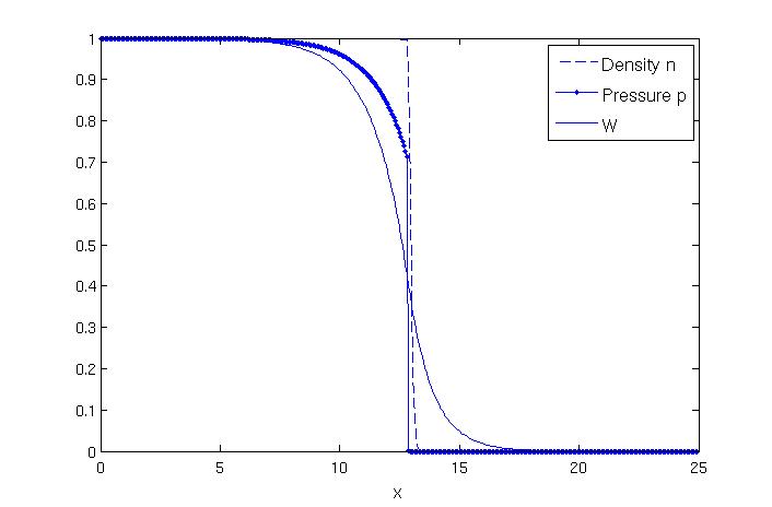
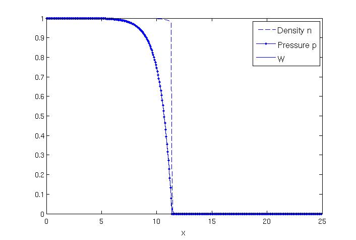
Figure 1: Plot of the density $n$ (dashed line), pressure $p$ (line with dot), $W$ (continuous line). Left : for $\nu=1$ and at final time $T=25\,s$. We notice a jump for the density from 0 to 1 at the front and a jump of the pressure. Right : for $\nu=0$ and at final time $T=12.5\,s$. In this case, we have $p=W$ and there is no jump on the pressure; moreover, the velocity of the front is faster. This observation is compatible with the interpretation that viscosity acts as a friction.

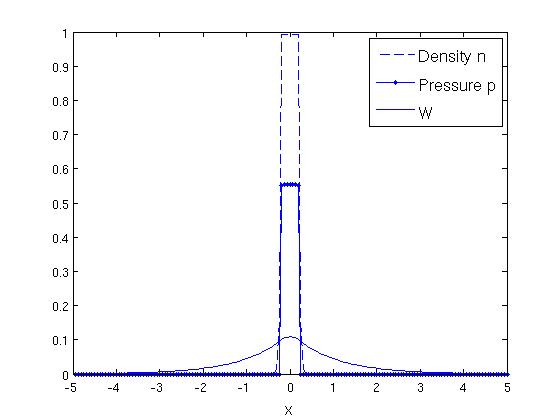
a) b)

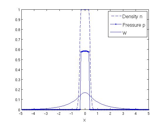
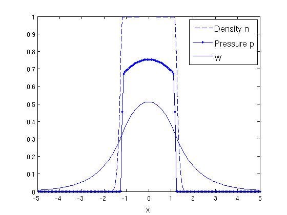
c) d)

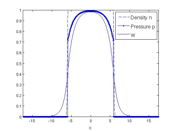
Figure 2: First steps of the formation of the propagating front with $k=100$ and $\nu=1$. The density $n$ (dashed line), the pressure $p$ (line with dot) and the potential $W$ (continuous line) are represented at 4 successives times : a) $t=0.1\,s$, b) $t=1.25\,s$, c) $t=3.75\,s$ and d) $t=12.5\,s$.

Numerical simulations. Finally, we present numerical simulations of the system (1)–(3) in one dimension. We use a discretization thanks to a cartesian grid of a bounded domain $[-L,L]$ of the real line. Equation (1) is discretized by a finite volume upwind scheme. Equation (2) is discretized thanks to finite difference scheme. Since we focus on the case where $k$ is large, we use $k=100$ in the numerical computation. For the initial data, we choose $n^{0}=\mathbf{1}_{[-0.2,0.2]}$. The growth function $G$ is chosen as in (48) with $P_{M}=1$.

In Figure 1, we display the shape of the density $n$, the pressure $p$ and $W$ obtained by the numerical simulation. The figure on the left displays the result with a viscosity coefficient $\nu=1$. For the comparison, we plot on the right of Figure 1, the shape in the case without viscosity ($\nu=0$). Comparing both figures, we observe that in the case $\nu=1$, we have a jump of the pressure at the interface of the solid tumor, whereas in the case $\nu=0$, the pressure is continuous at the interface.

We display in Figure 2 the first steps of the formation of the propagating front with the initial data $n^{0}=\mathbf{1}_{[-0.2,0.2]}$. For this simulation we take $\nu=1$ and $k=100$. The dynamics is represented thanks to the plot at 4 successives times of the density $n$, pressure $p$ and $W$. After a transitory regime during which the pressure increases until reaching its maximal value $P_{M}=1$, the shape of the traveling waves is obtained and the front of the tumor invades the healthy tissue.

4 Conclusion

A geometric model, also called incompressible, has been derived from a cell density model (also called compressible) when the pressure law is stiff. Because the viscosity is considered here, the limiting problem is a free boundary problem for the set $\Omega(t)$ of non-zero pressure. The limiting system for the pressure consists in an algebraic relation between the pressure $p_{\infty}$ and the limiting potential $W_{\infty}$ (17), coupled with an elliptic equation for the potential $W_{\infty}$ set in the whole space (15).

This is a major difference with the case where viscosity is neglected, the so-called Hele-Shaw system [15, 16]; then, the pressure is given by an elliptic equation for the pressure in the moving domain $\Omega(t)$. A paradox is that the effect of keeping viscosity generates a jump of the pressure at the interface of the region defining the tumor, unlike in [19, 18] where the Hele-Shaw problem is complemented with Dirichlet boundary conditions and therefore the pressure is continuous. This point is also observed in the numerical simulations in Section 3. The velocity of the propagating front of the tumor is given by the equation satisfied by the density (14). Because the pressure is discontinuous, it has weaker regularity that in the inviscid case treated in [19, 18] and we need to develop a new strategy of proof to derive the incompressible limit. Our approach is based on a kinetic formulation of the equation satisfied by the pressure.

This work also opens several additional questions. First, the case of general initial data is not treated here because we assume that $n^{0}$ vanishes outside $\Omega^{0}$. Then, it would be interesting to consider the case with active motion as in [18]. In such a case, equation (1) is replaced by a parabolic equation. Then the structure of the problem is different but the limiting system should be the same, except the equation for the density which implies then a faster propagation of the region $\Omega(t)$. Finally, it is formally clear from (10)–(12) that letting $\nu\to 0$, we recover the Hele-Shaw system. However, a rigorous proof of this fact requires compactness of the sequence which we is not directly available with the method developed here.

Acknowledgment. This work has been supported by the french ”ANR blanche” project Kibord: ANR-13-BS01-0004.

References

- [1] Nicholas D. Alikakos, Peter W. Bates and Xinfu Chen, Convergence of the Cahn-Hilliard Equation to the Hele-Shaw Model. Arch. Rational Mech. Anal. 128 (1994) 165–205.
- [2] G. Allaire, Homogenization of the Navier-Stokes equations and derivation of Brinkman’s law. In Applied Mathematics for Engineering Sciences, C. Carasso et al. eds., pp.7-20, Cépadués Editions, Toulouse (1991).
- [3] D. Ambrosi and L. Preziosi, On the closure of mass balance models for tumor growth. Math. Models Methods Appl. Sci., 12(5):737–754, 2002.
- [4] M. Basan, T. Risler, J.-F. Joanny, X. Sastre-Garau, and J. Prost, Homeostatic competition drives tumor growth and metastasis nucleation HFSP J. 3 (4), 265-72 (2009).
- [5] F. Ben Belgacem, P. E. Jabin, Compactness for nonlinear transport equations. J. Funct. Anal, 264 (2013), no. 1, 139–168.
- [6] T. Bittig, O. Wartlick, A. Kicheva, M. González-Gaitán, F. Jülicher, Dynamics of anisotropic tissue growth. New Journal of Physics 10 (2008) 063001.
- [7] D. Bresch, T. Colin, E. Grenier, B. Ribba and O. Saut, A viscolelastic model for avascular tumor growth. Disc. Cont. Dynam. Syst. Suppl. (2009) 101–108.
- [8] H. M Byrne, D. Drasdo, Individual-based and continuum models of growing cell populations: a comparison. J. Math. Biol. 58 (2009), no. 4-5, 657–687.
- [9] H. M. Byrne, J. R. King, D. L. S. McElwain, and L. Preziosi, A two-phase model of solid tumor growth. Appl. Math. Lett. (2003) 16: 567–573.
- [10] C. Chatelain, T. Balois, P. Ciarletta and M. Ben Amar, Emergence of microstructural patterns in skin cancer: a phase separation analysis in a binary mixture, New Journal of Physics 13 (2011) 115013.
- [11] V. Cristini, X. Li, J.S. Lowengrub, and S.M. Wise, Nonlinear simulations of solid tumor growth using a mixture model : invasion and branching. Journal of mathematical biology, 58(4) :723–763, 2009.
- [12] R. J. DiPerna and P.-L. Lions, Ordinary differential equations, transport theory and Sobolev spaces. Invent. Math., 98 (3) :511–547, 1989.
- [13] C. M. Elliotta and V. Janovský, A variational inequality approach to Hele-Shaw flow with a moving boundary. Proc. Roy. Soc. Edinburgh: Section A Mathematics, Vol. 88(1-2), 1981, 93–107.
- [14] Joachim Escher and Gieri Simonett, Classical solutions for Hele-Shaw models with surface tension. Adv. Differential Equations, 2(4):619–642, 1997.
- [15] A. Friedman, A hierarchy of cancer models and their mathematical challenges. DCDS(B) 4(1) (2004), 147–159.
- [16] J. S. Lowengrub, H. B. Frieboes, F. Jin, Y.-L. Chuang, X. Li, P. Macklin, S. M. Wise, V. Cristini, Nonlinear modelling of cancer: bridging the gap between cells and tumours. Nonlinearity 23 (2010), no. 1, R1–R91.
- [17] B. Perthame, A.-L. Dalibard, Existence of solutions of the hyperbolic Keller-Segel model. Trans. Amer. Math. Soc. 361 (2009), no. 5, 2319–2335.
- [18] B. Perthame, F. Quiròs, M. Tang, N. Vauchelet, Derivation of a Hele-Shaw type system from a cell model with active motion. Interfaces and Free Boundaries, in press.
- [19] B. Perthame, F. Quiròs and J.-L. Vàzquez, The Hele-Shaw asymptotics for mechanical models of tumor growth. Arch. Ration. Mech. Anal. 212 (2014), 93–127.
- [20] B. Perthame, M. Tang and N. Vauchelet, Traveling Wave Solution of the Hele-Shaw Model of Tumor Growth with Nutrient. M3AS, in press.
- [21] L. Preziosi, A. Tosin, Multiphase modelling of tumour growth and extracellular matrix interaction: mathematical tools and applications. J. Math. Biol. 58 (2009), no. 4-5, 625–656.
- [22] J. Ranft, M. Basana, J. Elgeti, J.-F. Joanny, J. Prost, F. Jülicher, Fluidization of tissues by cell division and apoptosis. Proc. Natl. Acad. Sci. USA (2010), no. 49, 20863–20868.
- [23] T. Roose, S. J. Chapman, P. K. Maini, Mathematical models of avascular tumor growth. SIAM Rev. 49 (2007), no. 2, 179–208.
- [24] J. Sherratt and M. Chaplain, A new mathematical model for avascular tumour growth. Journal of Mathematical Biology, 43(4):291–312, 2001.
- [25] M. Tang, N. Vauchelet, I. Cheddadi, I. Vignon-Clémentel, D. Drasdo, B. Perthame, Composite waves for a cell population system modelling tumor invasion. Chinese Annals of Math. Ser. B. Vol 34, no 2 (2013), 295–318.
- [26] X. Zheng, S. M. Wise and V. Cristini, Nonlinear simulation of tumor necrosis, neovascularization and tissue invasion via an adaptive finite-element/level-set method, Bull. Math. Biol. 67 (2005) 211–59.