The effect of concurrent geometry and roughness in interacting surfaces

Abstract

We study the interaction energy between two surfaces, one of them flat, the other describable as the composition of a small-amplitude corrugation and a slightly curved, smooth surface. The corrugation, represented by a spatially random variable, involves Fourier wavelengths shorter than the (local) curvature radii of the smooth component of the surface. After averaging the interaction energy over the corrugation distribution, we obtain an expression which only depends on the smooth component. We then approximate that functional by means of a derivative expansion, calculating explicitly the leading and next-to-leading order terms in that approximation scheme. We analyze the resulting interplay between shape and roughness corrections for some specific corrugation models in the cases of electrostatic and Casimir interactions.

I Introduction

The computation of interaction forces between close surfaces has been the subject of interest in many areas of physics, like colloidal and macromolecular phenomena, nuclear physics, electrostatics, van der Waals and Casimir interactions.

For the case of two surfaces which are ‘smooth’, namely, that have curvature radii much larger than the typical distance between them, there is a time-honored analytical tool to compute the total interaction force, the so-called Proximity Force Approximation (PFA) Derjaguin . This tool has, as its main virtue, that of delivering an answer in a rather straightforward fashion, usually in the form of an ordinary integral. Besides, it only demands two ingredients, the first being the knowledge of the force that would result in the same system if the two surfaces were infinite parallel plates (the simplest possible geometry). The second ingredient is the actual geometry of the two surfaces, i.e., part of the definition of the problem itself.

As it may be inferred from the previous remarks, the PFA satisfies a kind of ‘universality’, since the approach is essentially geometric. In fact, the underlying microscopic mechanism responsible for the force is only required at the stage of determining the force between parallel plates, the rest being dictated solely by the geometry of the surfaces. In other words, the PFA cannot distinguish (except for a global factor) between interactions which give place to the same force law between parallel plates.

Although it was originally presumed that the PFA should work reasonably well for close and gently curved surfaces, it has generally been assumed to be an uncontrolled approximation. Therefrom stemmed its major drawback: the absence of a procedure to asses its accuracy, since, for instance, a procedure to evaluate next to leading order (NTLO) corrections was lacking. In an attempt to deal with that limitation, in the last years we proposed, tested, and applied a new approximation scheme, the so-called Derivative Expansion (DE). Although originally introduced within the scope of the Casimir effect, for the calculation of the interaction energy between two smooth surfaces Foscoetal2011 , this approximation has been shown to be a natural extension of the PFA, and it has proven to be useful in rather different situations, not just for Casimir effect calculations Foscoetal2014 . The DE provides a systematic way of justifying the PFA and, under some circumstances, also of evaluating the NTLO corrections. One of the features that make the DE appealing is that the corrections are also geometric in nature, as in the PFA, and the result for the interaction can also be expressed as an integral. On the other hand the main difference is, naturally enough, that knowledge of the interaction for the case of parallel plates is not sufficient to determine the NTLO.

Although the DE approach may, and in fact has, been extended along many different directions pfaemig ; pfaemig2 ; pfaT ; pfaem , we shall consider here a generalization that may appear, at first sight, to be unnatural, since it corresponds to rough (in opposition to smooth) surfaces. However, we have in mind applying the DE to the smooth surfaces on top of which a rough component exists.

The influence of roughness on the interaction between surfaces has been studied in different contexts, mostly for cases where it has the form of a ripple on top of otherwise plane surfaces. This is a problem which arises, for example, in the electrostatic interaction framework, when calculating the capacitance of two (quasi) flat electrodes, to show that it increases in the presence of roughness Zhao . There is also an observable influence of roughness Mostep and periodic corrugations Intravaia2013 ; Banishev2013 in Casimir forces. In situations where the amplitude of roughness is much smaller than the distance between surfaces, the effect of roughness can be dealt with perturbatively li91 ; Neto2005 ; Schaden2014 , taking as zero order the interaction resulting for the smooth flat surfaces (defined to be the spatial averages of the rough ones).

There have been some attempts to analyze the concomitant effect of shape and roughness corrections on the interaction between surfaces. For instance, the particular case in which the asperities of the surface contains occasional high peaks and deep troughs, in addition to small-scale roughness, has been considered in Ref. Broer 2011 . The theoretical approach consisted in a perturbative evaluation of the small scale roughness combined with PFA for the large scale peaks and troughs. A related situation has been considered in Ref. Bimonte2013 . The system considered there consists in surfaces whose local separation is the sum of a slowly varying component due to overall shape, and a rapid part due to modulation. The calculations were performed using the PFA, and the approximations performed are tantamount to consider a two-step PFA, in which the effect of the rapid modulation is first considered for parallel plates, and the resulting interaction per unit area is used in a second step to take into account the slow changes in the overall shape. A similar geometry was considered in Ref. Banishev2013 , both from the theoretical and experimental points of view. The effect of the modulation was computed using the DE, and then the slowly varying shape using PFA. Interestingly enough, the experimental results confirm the NTLO corrections computed using the DE.

The aim of this paper is to compute the shape and roughness corrections systematically, looking for the existence of combined effects between them, beyond the PFA. Specifically, we will consider systems in which the geometry can be specified by defining just two surfaces: one of them, to be denoted by $L$, is assumed to be a plane, which (by a proper choice of orthogonal Cartesian coordinates), corresponds to the equation $x_{3}=0$ (we use $x_{1}$, $x_{2}$ and $x_{3}$ to denote such a choice). In terms of the same set of coordinates the other surface, $R$, can be defined as follows:

$$x_{3}\;=\;\Psi({\mathbf{x}_{\shortparallel}})\;\;,\;\;\;\;{\mathbf{x}_{\shortparallel}}\equiv(x_{1},x_{2})\;.$$ (1)

An important difference between this and previously considered applications of the DE, is that the function $\Psi({\mathbf{x}_{\shortparallel}})$ will not be regarded as necessarily smooth; rather, we characterize it by the property that it can be decomposed as the sum of two terms:

$$\Psi({\mathbf{x}_{\shortparallel}})\,=\,\psi({\mathbf{x}_{\shortparallel}})\,+\,\xi({\mathbf{x}_{\shortparallel}})\;,$$ (2)

where $\psi({\mathbf{x}_{\shortparallel}})$ is a smooth function, while $\xi({\mathbf{x}_{\shortparallel}})$ takes into account the ‘rough’ component of the surface.

We cannot apply the DE to non-smooth surfaces, but we will first average the interaction energy over the corrugation $\xi({\mathbf{x}_{\shortparallel}})$, and afterwards take into account the nontrivial geometry, characterized by the smooth function $\psi({\mathbf{x}_{\shortparallel}})$, this time by a legitimate use of the DE. Going beyond the leading order (PFA), we will be able to asses the relative weight of the roughness and shape corrections, including in the theoretical description the combined effect of both.

This paper is organized as follows: in Section II we derive general expressions for the leading and NTLO terms, for the DE of the functional representing the interaction energy between the two surfaces, up to the first non-trivial order in the correlation function $\Omega$. Section III contains a discussion of some general properties of the novel DE that contains the effect of roughness. Then in Section IV, we apply our general results to the case of the electrostatic interaction between two metallic surfaces at fixed electrostatic potentials. Section V deals with the DE for the interaction energy in the case of the Dirichlet and Neumann Casimir effects. Finally, in Section VI we present our conclusions.

II Derivative expansion for the interaction energy

II.1 Averaging out the corrugation

The corrugation function $\xi({\mathbf{x}_{\shortparallel}})$, introduced in Eq.(2), will be regarded as a random variable with null average:

$$\langle\xi({\mathbf{x}_{\shortparallel}})\rangle\;=\;0\;,$$ (3)

where $\langle\ldots\rangle$ denotes statistical average. Condition (3) can always be achieved, by a constant shift in $\psi$. For $n$ spatial arguments: ${\mathbf{x}^{(i_{1})}_{\shortparallel}},\ldots,{\mathbf{x}^{(i_{n})}_{\shortparallel}}$, statistical averages are defined by the functional integral:

$$\langle\xi({\mathbf{x}^{(i_{1})}_{\shortparallel}})\ldots\ldots\xi({\mathbf{x}^{(i_{n})}_{\shortparallel}})\rangle\;=\;\frac{\int{\mathcal{D}}\xi\;\xi({\mathbf{x}^{(i_{1})}_{\shortparallel}})\ldots\xi({\mathbf{x}^{(i_{n})}_{\shortparallel}})\,e^{-W[\xi]}}{\int{\mathcal{D}}\xi\,e^{-W[\xi]}}\;,$$ (4)

where $W[\xi]$ denotes a (real) not necessarily quadratic, functional of the corrugation function $\xi({\mathbf{x}_{\shortparallel}})$, determining the statistical weight of the different configurations.

Since we assume roughness to be small, to the first non trivial order in its amplitude, we shall only need the two-point autocorrelation function $\Omega$:

$$\Omega({\mathbf{x}_{\shortparallel}},{\mathbf{y}_{\shortparallel}})\;\equiv\;\langle\xi({\mathbf{x}_{\shortparallel}})\xi({\mathbf{y}_{\shortparallel}})\rangle\;,$$ (5)

since autocorrelation functions involving more than two $\xi$’s are of higher order in the amplitude. Note that, because of Eq.(3), $\Omega({\mathbf{x}_{\shortparallel}},{\mathbf{y}_{\shortparallel}})$ is a connected function of its arguments. In the quadratic $W[\xi]$ case,

$$W[\xi]\;=\;\frac{1}{2}\int_{{\mathbf{x}_{\shortparallel}},{\mathbf{y}_{\shortparallel}}}\xi({\mathbf{x}_{\shortparallel}})M({\mathbf{x}_{\shortparallel}},{\mathbf{y}_{\shortparallel}})\xi({\mathbf{y}_{\shortparallel}})\;,$$ (6)

where $M$ is a positive-definite kernel. In this case, one has

$$\Omega({\mathbf{x}_{\shortparallel}},{\mathbf{y}_{\shortparallel}})\;=\;M^{-1}({\mathbf{x}_{\shortparallel}},{\mathbf{y}_{\shortparallel}})\;.$$ (7)

At this point, we introduce an extra requirement, involving both $\Omega$ and $\psi$, the smooth component of $\Psi$: the autocorrelation length $l$, determined by $\Omega$, must be much smaller than the curvature radius of the smooth surface defined by $\psi$. Then, whenever the autocorrelation function differs appreciably from zero, the smooth surface can be regarded as approximately flat. In geometrical terms, the relevant pairs of arguments of $\Omega$ lie on the same tangent plane to each point of the $R$ surface. Hence, we only need to know the function $\Omega$, as an ingredient in the forthcoming calculations, for both arguments lying on the same plane surface, where it is translation-invariant (we assume the surfaces $R$ and $L$ to be homogeneous). Thus, we approximate $\Omega({\mathbf{x}_{\shortparallel}},{\mathbf{y}_{\shortparallel}})$ as follows:

$$\Omega({\mathbf{x}_{\shortparallel}},{\mathbf{y}_{\shortparallel}})\;\simeq\;\Omega({\mathbf{x}_{\shortparallel}}-{\mathbf{y}_{\shortparallel}})\;=\;\Omega(|{\mathbf{x}_{\shortparallel}}-{\mathbf{y}_{\shortparallel}}|)\;,$$ (8)

where the last equality follows from the (assumed) local isotropy of the curved surface.

The interaction between the two surfaces is a functional, $F[\Psi]$. However, we are not interested in the detailed dependence on $\Psi$, since that function contains the random, rapidly varying component, $\xi$. Our first step is then to average out the dependence on $\xi$ over its statistical distribution, obtaining a functional $F_{\rm eff}$, depending on $\psi$, the smooth part of $\Psi$:

$$F_{\rm eff}[\psi]\;\equiv\;\langle F[\psi+\xi]\rangle\;.$$ (9)

On the other hand, since the amplitude of $\xi$ is assumed to be small, we shall functionally expand $F$ in powers of $\xi$:

$$F_{\rm eff}[\psi] = \langle F[\psi]\,+\,\int_{{\mathbf{x}_{\shortparallel}}}F^{(1)}_{\psi}({\mathbf{x}_{\shortparallel}})\xi({\mathbf{x}_{\shortparallel}})+\frac{1}{2}\,\int_{{\mathbf{x}_{\shortparallel}},{\mathbf{y}_{\shortparallel}}}F^{(2)}_{\psi}({\mathbf{x}_{\shortparallel}},{\mathbf{y}_{\shortparallel}})\xi({\mathbf{x}_{\shortparallel}})\xi({\mathbf{y}_{\shortparallel}})$$ (10)

$$+ \frac{1}{3!}\,\int_{{\mathbf{x}_{\shortparallel}},{\mathbf{y}_{\shortparallel}},{\mathbf{z}_{\shortparallel}}}F^{(3)}_{\psi}({\mathbf{x}_{\shortparallel}},{\mathbf{y}_{\shortparallel}},{\mathbf{z}_{\shortparallel}})\,\xi({\mathbf{x}_{\shortparallel}})\xi({\mathbf{y}_{\shortparallel}})\xi({\mathbf{z}_{\shortparallel}})\rangle\,+\,\ldots$$

$$= F_{\rm eff,0}[\psi]\,+\,F_{\rm eff,2}[\psi]\,+\,F_{\rm eff,3}[\psi]\,+\,\ldots\;,$$

where the subindex $k$ in $F_{\rm eff,k}$ denotes $k^{th}$ order in $\xi$, the rugosity amplitude, and we have introduced the notation:

$$F^{(n)}_{\psi}({\mathbf{x}^{(1)}_{\shortparallel}},\ldots,{\mathbf{x}^{(n)}_{\shortparallel}})\;\equiv\;\frac{\delta^{n}F[\chi]}{\delta\chi({\mathbf{x}^{(1)}_{\shortparallel}})\ldots\delta\chi({\mathbf{x}^{(n)}_{\shortparallel}})}\Big{|}_{\chi=\psi}\;.$$ (11)

Clearly,

$$F_{\rm eff,0}[\psi]\;=\;F[\psi]\,$$ (12)

and

$$F_{\rm eff,2}[\psi]\;=\;\frac{1}{2}\,\int_{{\mathbf{x}_{\shortparallel}},{\mathbf{y}_{\shortparallel}}}F^{(2)}_{\psi}({\mathbf{x}_{\shortparallel}},{\mathbf{y}_{\shortparallel}})\,\Omega({\mathbf{y}_{\shortparallel}}-{\mathbf{x}_{\shortparallel}})\;.$$ (13)

Regarding the third and higher orders, in general they will require the knowledge of $n$-point correlation functions of the rugosity. An important exception is the Gaussian (quadratic) weight case, where only even numbers of fields yield non-vanishing contributions.

In Eq.(10), we will focus on the first two terms: the first, $F_{\rm eff,0}[\psi]$, is identical to the functional $F$ in the absence of corrugation, and the second, $F_{\rm eff,2}$, which contains the first nontrivial correction due to the small-amplitude corrugation. That small amplitude assumption justifies the inclusion of just the first order in $\Omega$ or, equivalently, the leading nontrivial order in the corrugation amplitude. Let us now proceed to perform the DE, to the second order in derivatives, for those two terms $F_{\rm eff,0}$ and $F_{\rm eff,2}$.

II.2 Derivative expansion for $F_{\rm eff}$

The averaged functional $F_{\rm eff}$, when expanded in derivatives up to the second order, should fall into an expression having the form Foscoetal2014

$$F_{\rm eff}[\psi]\;\simeq\;F_{\rm P}[\psi]\,+\,F_{\rm D}[\psi]\;,$$ (14)

where $F_{\rm P}[\psi]$, the term without derivatives, is just the PFA approximation to $F_{\rm eff}$:

$$F_{\rm P}[\psi]\;=\;\int d^{2}{\mathbf{x}_{\shortparallel}}\,V(\psi({\mathbf{x}_{\shortparallel}}))\;$$ (15)

and $F_{\rm D}$ denotes the term with two derivatives:

$$F_{\rm D}[\psi]\;=\;\int d^{2}{\mathbf{x}_{\shortparallel}}\,Z(\psi)|\nabla\psi|^{2}\;.$$ (16)

On the other hand, since $F_{\rm eff}$ has been expanded in powers of the corrugation, we shall have like expansions for $V$ and $Z$; namely,

$$V=V_{0}+V_{2}+\ldots\;\;,\;\;\;Z=Z_{0}+Z_{2}+\ldots\,,$$ (17)

and consequently

$$F_{\rm P}=F_{\rm P,0}+F_{\rm P,2}+\ldots\;\;,\;\;\;F_{\rm D}=F_{\rm D,0}+F_{\rm D,2}\,.$$ (18)

Here, the first terms in the expansion are independent of the corrugation, and therefore they can be obtained by applying the DE to the functional $F_{\rm eff,0}\equiv F$. Thus, the function $V_{0}$ can be determined, for example, from the value of $F$ for the special case of the parallel plates geometry:

$$V_{0}(a)\;=\;\frac{F[a]}{\mathcal{S}}\;,$$ (19)

where ${\mathcal{S}}$ denotes the area of the $L$ plate (this factor cancels out a similar one which appears in the numerator because of translation invariance on the plane when the plates are flat and parallel).

On the other hand, $Z_{0}$ can be determined from the knowledge of $F^{(2)}[\psi]$ for $\psi=a$ Foscoetal2011 ; Foscoetal2014 :

$$Z_{0}(a)\;=\;\frac{1}{4}\big{[}\Delta_{\mathbf{k}_{\shortparallel}}{\widetilde{f}}^{(2)}({\mathbf{k}_{\shortparallel}})\big{]}_{{\mathbf{k}_{\shortparallel}}\to 0}$$ (20)

with $\Delta_{\mathbf{k}_{\shortparallel}}\equiv\frac{\partial^{2}}{\partial k_{1}^{2}}+\frac{\partial^{2}}{\partial k_{2}^{2}}$, the Laplacian with respect to the momenta parallel to the $x_{3}={\rm constant}$ planes. Here, ${\widetilde{f}}^{(n)}$ is obtained from ${\widetilde{F}}_{a}^{(n)}({\mathbf{k}_{\shortparallel}}^{(1)},...,{\mathbf{k}_{\shortparallel}}^{(n)})$, the Fourier transform of $F_{a}^{(n)}$, by a procedure which we detail now. Since they are expansion coefficients defined around the translation-invariant configuration $x_{3}=a$, ${\widetilde{F}}_{a}^{(n)}$ must be proportional to the delta function of momentum conservation corresponding to each order. Thus,

$${\widetilde{F}}_{a}^{(n)}({\mathbf{k}_{\shortparallel}}^{(1)},...,{\mathbf{k}_{\shortparallel}}^{(n)})\;=\;(2\pi)^{2}\,\delta({\mathbf{k}_{\shortparallel}}^{(1)}+...+{\mathbf{k}_{\shortparallel}}^{(n)})\,{\widetilde{\gamma}}^{(n)}({\mathbf{k}_{\shortparallel}}^{(1)},...,{\mathbf{k}_{\shortparallel}}^{(n)})\;,$$ (21)

where ${\widetilde{\gamma}}^{(n)}$ is completely symmetric function of its arguments. However, the presence of the delta function means that it can be completely determined by a function of just $n-1$ arguments. To make that explicit, we introduce the kernels ${\widetilde{f}}^{(n)}$, as follows:

$${\widetilde{f}}^{(n)}({\mathbf{k}_{\shortparallel}}^{(1)},...,{\mathbf{k}_{\shortparallel}}^{(n-1)})\;\equiv\;{\widetilde{\gamma}}^{(n)}({\mathbf{k}_{\shortparallel}}^{(1)},...,{\mathbf{k}_{\shortparallel}}^{(n-1)},-\sum_{i=1}^{n-1}{\mathbf{k}_{\shortparallel}}^{(i)})\;,$$ (22)

among which we have the particular one appearing in the calculation of $Z_{0}$: ${\widetilde{f}}^{(2)}({\mathbf{k}_{\shortparallel}})\equiv{\widetilde{\gamma}}^{(2)}({\mathbf{k}_{\shortparallel}},-{\mathbf{k}_{\shortparallel}})$.

The function $Z_{0}(\psi)$ is then determined by the relation $Z_{0}(\psi)=Z_{0}(a)|_{a\to\psi}$.

Let us now consider the DE for $F_{\rm eff,2}$, the leading correction due to corrugation: the function $V_{2}$ is, again, conveniently obtained by evaluating $F_{\rm eff,2}$ for the case of parallel plates. Thus:

$$V_{2}(a)\;=\;\frac{F_{\rm eff,2}[a]}{\mathcal{S}}\;.$$ (23)

Recalling Eq.(13), we may give a more explicit formula for $V_{2}$. Indeed, from the relation:

$$F_{\rm eff,2}[a]\;=\;\frac{1}{2}\,\int_{{\mathbf{x}_{\shortparallel}},{\mathbf{y}_{\shortparallel}}}F_{a}^{(2)}({\mathbf{x}_{\shortparallel}},{\mathbf{y}_{\shortparallel}})\,\Omega({\mathbf{y}_{\shortparallel}}-{\mathbf{x}_{\shortparallel}})\;,$$ (24)

and noting that

$$F_{a}^{(2)}({\mathbf{x}_{\shortparallel}},{\mathbf{y}_{\shortparallel}})\,=\,\int\frac{d^{2}{\mathbf{p}_{\shortparallel}}}{(2\pi)^{2}}\,e^{i{\mathbf{p}_{\shortparallel}}\cdot({\mathbf{x}_{\shortparallel}}-{\mathbf{y}_{\shortparallel}})}{\widetilde{f}}^{(2)}({\mathbf{p}_{\shortparallel}})\;,$$ (25)

we get:

$$V_{2}(a)\;=\;\frac{1}{2}\,\int\frac{d^{2}{\mathbf{p}_{\shortparallel}}}{(2\pi)^{2}}\,{\widetilde{f}}^{(2)}({\mathbf{p}_{\shortparallel}})\,{\widetilde{\Omega}}({\mathbf{p}_{\shortparallel}})\;,$$ (26)

where ${\widetilde{\Omega}}$ is the Fourier transform of the autocorrelation function $\Omega$.

Finally, we obtain an explicit expression for $Z_{2}$. A rather straightforward approach would be to apply the analogue of Eq.(20), which was used for the functional $F$, now to the functional $F_{\rm eff,2}$, as defined in Eq.(13). Thus we see that:

$$Z_{2}(a)\;=\;\frac{1}{4}\big{[}\Delta_{\mathbf{k}_{\shortparallel}}{\widetilde{f}}_{2}^{(2)}({\mathbf{k}_{\shortparallel}})\big{]}_{{\mathbf{k}_{\shortparallel}}\to 0}\;,$$ (27)

where now ${\widetilde{f}}_{2}^{(2)}$ is evaluated from the functional expansion of $F_{\rm eff,2}$ in powers of $\eta$, to the second order in $\eta$. However, since $F_{\rm eff,2}$ is defined in terms of the second functional derivative of $F$, it is evident that ${\widetilde{f}}_{2}^{(2)}$ will involve the fourth order derivatives of $F$. Indeed, we obtain

$$Z_{2}(a)\;=\;\frac{1}{8}\,\int\frac{d^{2}{\mathbf{p}_{\shortparallel}}}{(2\pi)^{2}}\,\big{[}\Delta_{\mathbf{k}_{\shortparallel}}{\widetilde{f}}^{(4)}({\mathbf{p}_{\shortparallel}},-{\mathbf{p}_{\shortparallel}},{\mathbf{k}_{\shortparallel}})\big{]}_{{\mathbf{k}_{\shortparallel}}\to 0}\,{\widetilde{\Omega}}({\mathbf{p}_{\shortparallel}})\;,$$ (28)

with

$${\widetilde{f}}^{(4)}({\mathbf{k}_{\shortparallel}},{\mathbf{p}_{\shortparallel}},{\mathbf{q}_{\shortparallel}})\;=\;{\widetilde{\gamma}}^{(4)}({\mathbf{k}_{\shortparallel}},{\mathbf{p}_{\shortparallel}},{\mathbf{q}_{\shortparallel}},-{\mathbf{k}_{\shortparallel}}-{\mathbf{p}_{\shortparallel}}-{\mathbf{q}_{\shortparallel}})\;.$$ (29)

Thus, we have shown that the coefficients of the DE to second order for the leading correction in an expansion in powers of the corrugations requires a fourth order functional derivative of $F$. In other words, to evaluate the second order correction to the DE, to the leading order in the corrugation, we need the result for the fourth order term in the expansion of $F[a+\eta]$ in powers of $\eta$.

Before presenting the results that follow from the application of the general formulas to particular cases, we shall consider some of their general properties, based on dimensional analysis, combined with assumptions about the autocorrelation function $\Omega$ and about the curved surface.

III General properties

We note that, for a given interaction $F$, it will not be possible in general to find exact analytical expressions for $F_{P}$ and $F_{D}$, except for particular situations, or under under some simplifying assumptions. Since the interaction is determined, the two objects to play with are the autocorrelation function and the geometry.

On the other hand, having in mind cases where the geometry ($\psi$) is also given, it would be interesting to have a general formula for the DE, depending on an arbitrary $\Omega$, but where the geometry has been ‘integrated out’, namely, it appears only by means of the parameters characterizing the function $\psi$. For the term without derivatives, this can be achieved by using the so-called ‘height distribution function’. This representation can be obtained, for example, by introducing a ‘$1$’ inside the integral over ${\mathbf{x}_{\shortparallel}}$ in Eq.(15), written as follows: $1=\int_{0}^{\infty}da\,\delta(a-\psi({\mathbf{x}_{\parallel}}))$ (we assume $\psi>0$ everywhere). Thus,

$$F_{\rm P}[\psi]\;=\;\int_{0}^{\infty}da\,V(a)\,\sigma_{\rm P}(a)$$ (30)

where

$$\sigma_{\rm P}(a)\;=\;\int d^{2}{\mathbf{x}_{\shortparallel}}\,\delta(a-\psi({\mathbf{x}_{\parallel}}))\;.$$ (31)

We see that the geometry, for this term, is encoded in $\sigma_{P}$, while the part dependent on the interaction and the corrugation is contained in $V(a)$. More explicitly,

$$F_{\rm P}[\psi]\;=\;\frac{1}{2}\,\int\frac{d^{2}{\mathbf{p}_{\shortparallel}}}{(2\pi)^{2}}\,{\widetilde{\Omega}}({\mathbf{p}_{\shortparallel}})\,\int_{0}^{\infty}da\,{\widetilde{f}}^{(2)}({\mathbf{p}_{\shortparallel}})\,\sigma_{\rm P}(a)\;.$$ (32)

For the term with two derivatives, a similar procedure to the one applied above yields:

$$F_{\rm D}[\psi]\;=\;\int_{0}^{\infty}da\,Z(a)\,\sigma_{\rm D}(a)$$ (33)

with

$$\sigma_{\rm D}(a)\;=\;\int d^{2}{\mathbf{x}_{\shortparallel}}\,\delta(a-\psi({\mathbf{x}_{\parallel}}))|\nabla\psi({\mathbf{x}_{\shortparallel}})|^{2}\;,$$ (34)

where now the geometry of the curved plate appears in the $\sigma_{D}$ function, similar to the height distribution function, but weighted with the square of the gradient of $\psi$. Thus:

$$F_{\rm D}[\psi]\;=\;\frac{1}{8}\,\int\frac{d^{2}{\mathbf{p}_{\shortparallel}}}{(2\pi)^{2}}\,{\widetilde{\Omega}}({\mathbf{p}_{\shortparallel}})\,\int_{0}^{\infty}da\,\big{[}\Delta_{\mathbf{k}_{\shortparallel}}{\widetilde{f}}^{(4)}({\mathbf{p}_{\shortparallel}},-{\mathbf{p}_{\shortparallel}},{\mathbf{k}_{\shortparallel}})\big{]}_{{\mathbf{k}_{\shortparallel}}\to 0}\,\sigma_{\rm D}(a)\;.$$ (35)

To simplify the forthcoming discussion, we use dimensional analysis whenever possible. To that end, we note that the mass dimensions of the objects appearing in the general formulas can be determined as soon as we assume that $F$ is an energy; thus we have $[F]=[M]$, ${\widetilde{\Omega}}=[M]^{-4}$, $[{\widetilde{f}}^{(2)}]=[M]^{5}$, and $[{\widetilde{f}}^{(4)}]=[M]^{7}$. Therefore, the momentum-space Laplacian of $[{\widetilde{f}}^{(4)}]$ has dimensions $[M]^{5}$. We then rewrite $V$ and $Z$ using dimensionless objects. For the PFA contribution, there is not much to be said for $V_{0}(a)$ beyond expression (19); thus,

$$V_{0}(a)\;=\;a^{-3}\;\left(\frac{a^{3}F[a]}{\mathcal{S}}\right)$$ (36)

while for $V_{2}$, which is given by a momentum integral, we introduce a dimensionless momentum ${\mathbf{l}_{\shortparallel}}$, attained by the rescaling ${\mathbf{p}_{\shortparallel}}={\mathbf{l}_{\shortparallel}}/a$:

$$V_{2}(a)\;=\;a^{-3}\;\;\frac{1}{2}\,\int\frac{d^{2}{\mathbf{l}_{\shortparallel}}}{(2\pi)^{2}}\,{\widetilde{g}}^{(2)}({\mathbf{l}_{\shortparallel}})\,{\widetilde{\omega}}({\mathbf{l}_{\shortparallel}})\;,$$ (37)

where we have introduced the dimensionless functions:

$${\widetilde{g}}^{(2)}({\mathbf{l}_{\shortparallel}})\,=\,a^{5}\,{\widetilde{f}}^{(2)}({\mathbf{l}_{\shortparallel}}/a)\;\;,\;\;\;{\widetilde{\omega}}({\mathbf{l}_{\shortparallel}})\,=\,a^{-4}\,{\widetilde{\Omega}}({\mathbf{l}_{\shortparallel}}/a)\;.$$ (38)

Thus, to the order we are considering here, we have,

$$V(a)\;=\;a^{-3}\;\;\left[\frac{a^{3}F[a]}{\mathcal{S}}+\frac{1}{2}\,\int\frac{d^{2}{\mathbf{l}_{\shortparallel}}}{(2\pi)^{2}}\,{\widetilde{g}}^{(2)}({\mathbf{l}_{\shortparallel}})\,{\widetilde{\omega}}({\mathbf{l}_{\shortparallel}})\right]\;.$$ (39)

Regarding $Z_{2}$, which involves ${\widetilde{\Omega}}$ and ${\widetilde{f}}^{(4)}$, a similar rescaling yields:

$$Z_{2}(a)\;=\;a^{-3}\;\;\frac{1}{8}\,\int\frac{d^{2}{\mathbf{l}_{\shortparallel}}}{(2\pi)^{2}}\,{\widetilde{h}}^{(2)}({\mathbf{l}_{\shortparallel}})\,{\widetilde{\omega}}({\mathbf{l}_{\shortparallel}})\;,$$ (40)

where

$${\widetilde{h}}^{(2)}({\mathbf{l}_{\shortparallel}})\;=\;a^{5}\,\big{[}\Delta_{{\mathbf{k}_{\shortparallel}}/a}{\widetilde{f}}^{(4)}({\mathbf{l}_{\shortparallel}}/a,-{\mathbf{l}_{\shortparallel}}/a,{\mathbf{k}_{\shortparallel}}/a)\big{]}_{{\mathbf{k}_{\shortparallel}}\to 0}\;.$$ (41)

Let us consider some exact properties and results that can be obtained about the contributions due to $V_{2}$ and $Z_{2}$, as well as about the interplay between roughness and geometry under some simplifying assumptions about the autocorrelation function. Although the resulting models will not necessarily correspond to realistic situations, they have the advantage that some insight about the interplay between the different causes may be elucidated more clearly.

1. Sharp cutoff model: This model corresponds to the autocorrelation function:

   $${\widetilde{\Omega}}({\mathbf{p}_{\shortparallel}})\;=\;\frac{4\pi\epsilon^{2}}{p_{\rm max}^{2}-p_{\rm min}^{2}}\,\theta(|{\mathbf{p}_{\shortparallel}}|-p_{\rm min})\,\theta(p_{\rm max}-|{\mathbf{p}_{\shortparallel}}|)\;,$$ (42)

   where $p_{\rm max}\geq p_{\rm min}\geq 0$, and $\epsilon$ is a constant with the dimensions of a length, which is a measure of the amplitude of the corrugation (its rms value). The constants $p_{\rm max}$ and $p_{\rm min}$ play the role of UV and IR cutoffs, respectively. Equivalently, they determine the minimum and maximum correlation distances.

   In this model, we see that the second order contribution to the PFA approximation becomes:

   $$F_{\rm P,2}=\int d^{2}{\mathbf{x}_{\shortparallel}}V_{2}=\frac{\epsilon^{2}}{p_{\rm max}^{2}-p_{\rm min}^{2}}\,\int_{0}^{\infty}da\,\frac{\sigma_{\rm P}(a)}{a^{7}}\,\int_{ap_{\rm min}}^{ap_{\rm max}}dx\,x{\widetilde{g}}^{(2)}(x)\;.$$ (43)

   On the other hand, for the term with two derivatives, determined by $Z_{2}$, the equivalent expression is:

   $$F_{\rm D,2}=\int d^{2}{\mathbf{x}_{\shortparallel}}Z_{2}|\nabla\psi|^{2}=\frac{\epsilon^{2}}{4(p_{\rm max}^{2}-p_{\rm min}^{2})}\,\int_{0}^{\infty}da\,\frac{\sigma_{\rm D}(a)}{a^{7}}\,\int_{ap_{\rm min}}^{ap_{\rm max}}dx\,x\,{\widetilde{h}}^{(2)}(x)\;.$$ (44)

2. $\delta$-like ${\widetilde{\Omega}}$: This case corresponds to a limit of the sharp-cutoff model, such that the two cutoffs collapse to a common value $q$. Thus, the momentum-space autocorrelation function has the following form:

   $${\widetilde{\Omega}}({\mathbf{p}_{\shortparallel}})\;=\;2\pi\epsilon^{2}\,\frac{\delta(|{\mathbf{p}_{\shortparallel}}|-q)}{|{\mathbf{p}_{\shortparallel}}|}\;,$$ (45)

   again, $\epsilon$ is a length, which may be interpreted as a measure of the amplitude of the corrugation, while ${\mathbf{q}_{\shortparallel}}$ determines its momentum scale. Thus,

   $$\int d^{2}{\mathbf{x}_{\shortparallel}}V_{2}\;=\;\frac{\epsilon^{2}}{2}\,\int_{0}^{\infty}da\,\sigma_{\rm P}(a)\,{\widetilde{f}}^{(2)}(q)\,=\,\frac{\epsilon^{2}}{2}\,\int_{0}^{\infty}da\,\frac{\sigma_{\rm P}(a)}{a^{5}}\,{\widetilde{g}}^{(2)}(qa)\;$$ (46)

   and

   $$\int d^{2}{\mathbf{x}_{\shortparallel}}Z_{2}|\nabla\psi|^{2}\;=\;\frac{\epsilon^{2}}{8}\,\int_{0}^{\infty}da\,\sigma_{\rm D}(a)\,{\widetilde{g}}^{(2)}(q)\,=\,\frac{\epsilon^{2}}{8}\,\int_{0}^{\infty}da\,\frac{\sigma_{\rm D}(a)}{a^{5}}\,{\widetilde{h}}^{(2)}(qa)\;.$$ (47)

3. Momentum-independent correlation function:

   Finally, this situation corresponds to a case where the IR cutoff tends to zero and the UV one to infinity. Equivalently, there is a vanishing correlation length. Thus

   $${\widetilde{\Omega}}({\mathbf{k}_{\shortparallel}})\;=\;{\widetilde{\Omega}}_{0}\,\equiv\,{\rm constant}\;,$$ (48)

   where ${\widetilde{\Omega}}_{0}$ has the dimensions of $({\rm length})^{4}$. Note that this value of ${\widetilde{\Omega}}_{0}$ may be thought of as a particular limit of the two cutoff case, such that the product of $\epsilon$ by $p_{\rm max}-p_{\rm min}$ remains constant.

   Then we see that:

   $$V_{2}(a)\;=\;\frac{{\widetilde{\Omega}}_{0}}{2a^{7}}\;\int\frac{d^{2}{\mathbf{l}_{\shortparallel}}}{(2\pi)^{2}}\,{\widetilde{g}}^{(2)}({\mathbf{l}_{\shortparallel}})\,.$$ (49)

   and

   $$Z_{2}(a)\;=\;\frac{{\widetilde{\Omega}}_{0}}{8a^{7}}\;\int\frac{d^{2}{\mathbf{l}_{\shortparallel}}}{(2\pi)^{2}}\,{\widetilde{h}}^{(2)}({\mathbf{l}_{\shortparallel}})\;.$$ (50)

   For the particular case of interactions which do not introduce any dimensionful quantity into the problem (except $a$), like in the Casimir effect for a scalar field with Dirichlet or Neumann conditions, or even the case of the electromagnetic field, the dimensionless kernels which appear integrated above are just numbers. Thus, in those cases we shall have, regarding the dependence with a,

   $$V_{2}(a)\;\propto\;\frac{1}{a^{7}}\;\;,\;\;\;Z_{2}(a)\;\propto\;\frac{1}{a^{7}}\;.$$ (51)

   An important remark is that no boundary condition is perfect for all momenta, therefore one should also expect an UV cutoff to exist in ${\widetilde{g}}^{2}$ and ${\widetilde{h}}^{2}$. Thus, the momentum integrals above shall have cutoffs (in principle, unrelated to the ones of the autocorrelation function). This should be kept in mind, in particular, when the integrals over ${\mathbf{l}_{\shortparallel}}$ are UV divergent. In this situation, the behaviour in Eq.(51) should be reliable when $a$ is much larger than the inverse of the UV cutoff. For small values of $a$, however, one should expect a smoother behaviour than that of Eq.(51).

Finally, in order to gain some insight, and because it is representative of many relevant situations, we evaluate the geometrical factors $\sigma_{\rm P}$ and $\sigma_{\rm D}$ explicitly for the case of two particular surfaces which produce relatively simple results.

The first case we consider has revolution symmetry around the $x_{3}$ axis and is defined by the function $\psi=d+b|{\mathbf{x}_{\shortparallel}}|^{\kappa}$, where $d$, $b$ and $\kappa$ are positive constants. We obtain:

$$\sigma_{\rm P}(a)\;=\;\left\{\begin{array}[]{ccc}0&{\rm if}&a<d\\ \frac{2\pi}{b\kappa}(\frac{a-d}{b})^{\frac{2}{\kappa}-1}&{\rm if}&a\geq d\end{array}\right.$$ (52)

and

$$\sigma_{\rm D}(a)\;=\;\left\{\begin{array}[]{ccc}0&{\rm if}&a<d\\ 2\pi\kappa(a-d)&{\rm if}&a\geq d\end{array}\right.\;.$$ (53)

The other case corresponds to a sphere of radius to be $R$ and its distance of closest approach to the flat surface to be $d$, we find:

$$\sigma_{\rm P}(a)\;=\;\left\{\begin{array}[]{cc}2\pi R(1-\frac{a}{R}+\frac{d}{R})&{\rm if}\;d\leq a\leq R+d\\ 0&{\rm otherwise}\end{array}\right.$$ (54)

and

$$\sigma_{\rm D}(a)\;=\;\left\{\begin{array}[]{cc}2\pi(a-d)(1+\frac{1}{1-\frac{a}{R}+\frac{d}{R}})&{\rm if}\;d\leq a\leq R+d-\sqrt{R^{2}-\rho_{M}^{2}}\\ 0&{\rm otherwise}\end{array}\right.$$ (55)

where $\rho_{M}<R$ is a spatial cutoff, required for the term with two derivatives to discard contributions where the approximation is not valid (since the derivative of $\psi$ diverges).

In the next sections, we apply the previous general expressions for the DE corresponding to $F_{\rm eff,2}$ to two interesting cases: the electrostatic interaction of two metallic surfaces held at fixed electrostatic potentials (Section IV), and the Casimir interaction between two Dirichlet or Neumann surfaces acting on a quantum massless real scalar field (Section V).

IV Results for the electrostatic case

In this section, we apply the general results for the interaction energy between surfaces to the particular case of the electrostatic interaction between two perfect conductors held at a potential difference $V$. The electrostatic energy will be denoted by $U$ and is given by

$$U[\Psi]=\frac{\epsilon_{0}V^{2}}{2}\int d^{2}{\mathbf{x}_{\shortparallel}}\int_{0}^{\Psi}dx_{3}|\nabla\phi|^{2}\,,$$ (56)

where $\phi({\mathbf{x}_{\shortparallel}},x_{3})$ is the electrostatic potential, that satisfies the Laplace equation between plates, subjected to the boundary conditions $\phi({\mathbf{x}_{\shortparallel}},0)=0$ and $\phi({\mathbf{x}_{\shortparallel}},\Psi)=V$. As described in previous sections, in order to obtain the derivative expansion for $U_{eff}[\psi]=<U[\psi+\xi]>$ it is necessary to compute the fourth order functional derivative of $U$ at $\Psi=a$. Therefore we write

$$\Psi=a+\eta({\mathbf{x}_{\shortparallel}})$$ (57)

and expand the electrostatic energy up to the fourth order in $\eta$. In a previous work annphys , we performed this calculation up to second order. We will follow a similar approach here, extending the results to the fourth order case.

We expand the boundary condition on the curved surface in powers of $\eta$:

$$V=\phi({\mathbf{x}_{\shortparallel}},a)+\eta({\mathbf{x}_{\shortparallel}})\partial_{3}\phi({\mathbf{x}_{\shortparallel}},a)+\frac{\eta^{2}({\mathbf{x}_{\shortparallel}})}{2}\partial_{3}^{2}\phi({\mathbf{x}_{\shortparallel}},a)+\frac{\eta^{3}({\mathbf{x}_{\shortparallel}})}{6}\partial_{3}^{3}\phi({\mathbf{x}_{\shortparallel}},a)+....$$ (58)

and look for solutions of the form

$$\phi({\mathbf{x}_{\shortparallel}},x_{3})=\sum_{n\geq 0}\phi^{(n)}({\mathbf{x}_{\shortparallel}},x_{3})\,,$$ (59)

where $\phi^{(n)}({\mathbf{x}_{\shortparallel}},x_{3})$ is $O(\eta^{n})$ and satisfies the Laplace equation. The boundary conditions are $\phi^{(n)}({\mathbf{x}_{\shortparallel}},0)=0$ and

$$\phi^{(0)}({\mathbf{x}_{\shortparallel}},a) = V$$

$$\phi^{(1)}({\mathbf{x}_{\shortparallel}},a) = -\eta({\mathbf{x}_{\shortparallel}})\partial_{3}\phi^{(0)}({\mathbf{x}_{\shortparallel}},a)$$

$$\phi^{(2)}({\mathbf{x}_{\shortparallel}},a) = -\eta({\mathbf{x}_{\shortparallel}})\partial_{3}\phi^{(1)}({\mathbf{x}_{\shortparallel}},a)-\frac{\eta^{2}({\mathbf{x}_{\shortparallel}})}{2}\partial_{3}^{2}\phi^{(0)}({\mathbf{x}_{\shortparallel}},a)$$

$$\ \phi^{(3)}({\mathbf{x}_{\shortparallel}},a) = -\eta({\mathbf{x}_{\shortparallel}})\partial_{3}\phi^{(2)}({\mathbf{x}_{\shortparallel}},a)-\frac{\eta^{2}({\mathbf{x}_{\shortparallel}})}{2}\partial_{3}^{2}\phi^{(1)}({\mathbf{x}_{\shortparallel}},a)\,,$$ (60)

as can be readily checked by inserting the expansion Eq.(59) into Eq.(58).

The leading order solution is of course $\phi^{(0)}=Vx_{3}/a$. Taking into account the boundary condition at $x_{3}=0$ we have, for $n\geq 1$,

$$\phi^{(n)}({\mathbf{x}_{\shortparallel}},x_{3})=\int\frac{d^{2}{\mathbf{k}_{\shortparallel}}}{(2\pi)^{2}}\,e^{i{\mathbf{k}_{\shortparallel}\cdot x_{\shortparallel}}}A^{(n)}({\mathbf{k}_{\shortparallel}})\sinh(k_{\shortparallel}x_{3})\,,$$ (61)

where the functions $A^{(n)}({\mathbf{k}_{\shortparallel}})$ are determined by the boundary conditions at $x_{3}=a$:

$$A^{(1)}({\mathbf{k}_{\shortparallel}}) = -\frac{V}{a}\frac{\tilde{\eta}({\mathbf{k}_{\shortparallel}})}{\sinh(k_{\shortparallel}a)}$$

$$A^{(2)}({\mathbf{k}_{\shortparallel}}) = \frac{V}{a\sinh(k_{\shortparallel}a)}\int\frac{d^{2}{\mathbf{p}_{\shortparallel}}}{(2\pi)2}p_{\shortparallel}\coth(p_{\shortparallel}a)\tilde{\eta}({\mathbf{k}_{\shortparallel}}+{\mathbf{p}_{\shortparallel}})\tilde{\eta}(-{\mathbf{p}_{\shortparallel}})$$

$$A^{(3)}({\mathbf{k}_{\shortparallel}}) = \frac{V}{a\sinh(k_{\shortparallel}a)}\int\frac{d^{2}{\mathbf{p}_{\shortparallel}}}{(2\pi)^{2}}\frac{d^{2}{\mathbf{p}_{\shortparallel}}}{(2\pi)^{2}}\tilde{\eta}({\mathbf{k}_{\shortparallel}}+{\mathbf{q}_{\shortparallel}})\tilde{\eta}({\mathbf{p}_{\shortparallel}}-{\mathbf{q}_{\shortparallel}})\tilde{\eta}(-{\mathbf{p}_{\shortparallel}})$$ (62)

$$\quad\quad\quad\quad\times(p_{\shortparallel}q_{\shortparallel}\coth(p_{\shortparallel}a)\coth(q_{\shortparallel}a)-\frac{1}{2}|{\mathbf{q}_{\shortparallel}}-{\mathbf{p}_{\shortparallel}}|^{2})\,.$$

After a long but straightforward calculation, the expansion of the electrostatic energy reads

$$U[a+\eta]=\sum_{n\geq 0}U^{(n)}[a+\eta]$$ (63)

with

$$U^{(0)} = \frac{\epsilon_{0}V^{2}}{2a}\int d^{2}{\mathbf{x}_{\shortparallel}}$$

$$U^{(1)} = -\frac{\epsilon_{0}V^{2}}{2a^{2}}\int d^{2}{\mathbf{x}_{\shortparallel}}\eta$$

$$U^{(2)} = \frac{\epsilon_{0}V^{2}}{2a^{2}}\int\frac{d^{2}{\mathbf{k}_{\shortparallel}}}{(2\pi)^{2}}k_{\shortparallel}\coth(k_{\shortparallel}a)\tilde{\eta}({\mathbf{k}_{\shortparallel}})\tilde{\eta}(-{\mathbf{k}_{\shortparallel}})$$

$$U^{(3)} = \frac{1}{3!}\int\frac{d^{2}{\mathbf{k}_{\shortparallel}}}{(2\pi)^{2}}\frac{{d^{2}{\mathbf{p}_{\shortparallel}}}}{{(2\pi)^{2}}}\tilde{f}^{(3)}({\mathbf{k}_{\shortparallel}},{\mathbf{p}_{\shortparallel}})\,\tilde{\eta}({\mathbf{k}_{\shortparallel}})\tilde{\eta}({\mathbf{p}_{\shortparallel}})\tilde{\eta}(-{\mathbf{k}_{\shortparallel}}-{\mathbf{p}_{\shortparallel}})$$

$$U^{(4)} = \frac{1}{4!}\int\frac{d^{2}{\mathbf{k}_{\shortparallel}}}{(2\pi)^{2}}\frac{{d^{2}{\mathbf{p}_{\shortparallel}}}}{{(2\pi)^{2}}}\frac{d^{2}{\mathbf{q}_{\shortparallel}}}{(2\pi)^{2}}\tilde{f}^{(4)}({\mathbf{k}_{\shortparallel}},{\mathbf{p}_{\shortparallel}},{\mathbf{q}_{\shortparallel}})\,\tilde{\eta}({\mathbf{k}_{\shortparallel}})\tilde{\eta}({\mathbf{p}_{\shortparallel}})\tilde{\eta}({\mathbf{q}_{\shortparallel}})\tilde{\eta}(-{\mathbf{k}_{\shortparallel}}-{\mathbf{p}_{\shortparallel}}-{\mathbf{q}_{\shortparallel}})\,.$$ (64)

The explicit expressions for the functions $\tilde{f}^{(n)}$ are

$$\tilde{f}^{(3)}({\mathbf{k}_{\shortparallel}},{\mathbf{p}_{\shortparallel}}) = -\frac{3\epsilon_{0}V^{2}}{a^{2}}\left({\mathbf{k}_{\shortparallel}}\cdot{\mathbf{p}_{\shortparallel}}+k_{\shortparallel}p_{\shortparallel}\coth(k_{\shortparallel}a)\coth(p_{\shortparallel}a)\right)$$

$$\tilde{f}^{(4)}({\mathbf{k}_{\shortparallel}},{\mathbf{p}_{\shortparallel}},{\mathbf{q}_{\shortparallel}}) = \frac{2\epsilon_{0}V^{2}}{a^{2}}\bigg{(}\big{(}h({\mathbf{k}_{\shortparallel}},{\mathbf{p}_{\shortparallel}},{\mathbf{q}_{\shortparallel}})+h({\mathbf{k}_{\shortparallel}},{\mathbf{q}_{\shortparallel}},{\mathbf{p}_{\shortparallel}})+h({\mathbf{p}_{\shortparallel}},{\mathbf{k}_{\shortparallel}},{\mathbf{q}_{\shortparallel}})$$ (65)

$$+ h({\mathbf{p}_{\shortparallel}},{\mathbf{q}_{\shortparallel}},{\mathbf{k}_{\shortparallel}})+h({\mathbf{q}_{\shortparallel}},{\mathbf{p}_{\shortparallel}},{\mathbf{k}_{\shortparallel}})+h({\mathbf{q}_{\shortparallel}},{\mathbf{k}_{\shortparallel}},{\mathbf{p}_{\shortparallel}})\big{)}\bigg{)}\,,$$

with

$$h({\mathbf{k}_{\shortparallel}},{\mathbf{p}_{\shortparallel}},{\mathbf{q}_{\shortparallel}})=q_{\shortparallel}\coth(q_{\shortparallel}a)(2q_{\shortparallel}^{2}-{\mathbf{k}_{\shortparallel}}\cdot{\mathbf{q}_{\shortparallel}})+p_{\shortparallel}q_{\shortparallel}|{\mathbf{k}_{\shortparallel}}+{\mathbf{p}_{\shortparallel}}|\coth(p_{\shortparallel}a)\coth(q_{\shortparallel}a)\coth(|{\mathbf{k}_{\shortparallel}}+{\mathbf{p}_{\shortparallel}}|a)\,.$$ (66)

In order to obtain these results it is necessary to expand the electrostatic energy in powers of $\eta$, taking into account not only the expansion of the potential but also the upper limit of integration in Eq.(56).

As a partial check of our results, we can evaluate the electrostatic energy for a constant perturbation

$$\eta({\mathbf{x}_{\shortparallel}})=\eta_{0}\Rightarrow\tilde{\eta}({\mathbf{k}_{\shortparallel}})=\eta_{0}(2\pi)^{2}\delta({\mathbf{k}_{\shortparallel}})$$ (67)

to obtain

$$U\approx\frac{\epsilon_{0}V^{2}}{2}\frac{\mathcal{S}}{a}\big{(}1-\frac{\eta_{0}}{a}+\frac{\eta_{0}^{2}}{a^{2}}-\frac{\eta_{0}^{3}}{a^{3}}+\frac{\eta_{0}^{4}}{a^{4}}\big{)}\,,$$ (68)

which is the expansion of the exact result $\epsilon_{0}V^{2}{\mathcal{S}/(2(a+\eta_{0}))}$ up to fourth order in the perturbation.

From the expression for $U^{(2)}$ given in Eq.(64) one can read the explicit form for $\tilde{f}^{(2)}({\mathbf{k}_{\shortparallel}})$. Using Eq.(26) we obtain

$$V_{2}(a)=\frac{\epsilon_{0}V^{2}}{2\pi a^{5}}\int_{0}^{\infty}dl_{\shortparallel}\,l_{\shortparallel}^{2}\,\tilde{\Omega}(l_{\parallel}/a)\coth l_{\shortparallel}\,\,.$$ (69)

The function $Z_{2}$ can be obtained combining the expression for $U^{(4)}$ in Eq.(64) with Eq.(28). The result is

$$Z_{2}(a)=\frac{2\epsilon_{0}V^{2}}{\pi a^{5}}\int dl_{\shortparallel}\,l_{\shortparallel}\tilde{\Omega}(l_{\shortparallel}/a)B(l_{\shortparallel})$$ (70)

where

$$B(l_{\shortparallel})=1+(l_{\shortparallel}\coth l_{\shortparallel}+l_{\shortparallel}^{2}\coth^{2}l_{\shortparallel})(\frac{1}{6}+\frac{1}{8l_{\shortparallel}}(\coth l_{\shortparallel}+\frac{l_{\shortparallel}}{\sinh^{2}l_{\shortparallel}}(2l_{\shortparallel}\coth l_{\shortparallel}-3))\,.$$ (71)

IV.1 Sphere-plane geometry

Let us now consider the sphere-plane geometry, assuming a sharp-cutoff model for the roughness. It is easy to obtain analytic results for sufficiently large values of $p_{\rm max}d$. Indeed, inserting Eq.(42) into Eq.(69) we obtain

$$V_{2}(a)\simeq\frac{2}{3a^{2}}\epsilon_{0}V^{2}\epsilon^{2}p_{\rm max}\,,$$ (72)

where we have assumed that the integral in Eq.(69) is dominated by large values of the momentum. A similar analysis can be done for $Z_{2}(a)$. Inserting Eq.(42) into Eq.(70) we get

$$Z_{2}(a)\simeq\frac{1}{3a}\epsilon_{0}V^{2}\epsilon^{2}p_{\rm max}^{2}\,.$$ (73)

The roughness correction to the interaction energy in this geometry can be computed using the height distribution functions introduced in the previous section

$$U_{P,2} = \int_{0}^{\infty}\sigma_{P}(a)V_{2}(a)$$

$$U_{D,2} = \int_{0}^{\infty}\sigma_{D}(a)Z_{2}(a)\,.$$ (74)

Taking the derivative of the interaction energy with respect to the sphere-plane distance $d$ one can obtain the corresponding corrections to the force, that will be denoted by ${\cal F}_{P,2}$ and ${\cal F}_{D,2}$ respectively. The results are

$${\mathcal{F}}_{P,2} = -\frac{4}{3d^{2}}\pi R\epsilon_{0}V^{2}\epsilon^{2}p_{\rm max}\left(1-\frac{d}{R}\right)$$

$${\mathcal{F}}_{D,2} = \frac{4}{3}\pi\epsilon_{0}V^{2}\epsilon^{2}p_{\rm max}^{2}\log(d/R)\,,$$ (75)

where we have made an expansion for small values of $d/R$.

On the other hand, the corresponding result for smooth sphere-plane surfaces is given by annphys

$${\cal F}_{P,0}+{\cal F}_{D,0}=-\frac{\pi\epsilon_{0}V^{2}R}{d}-\frac{\pi}{3}\epsilon_{0}V^{2}\log(d/R)\,.$$ (76)

The ratio between the leading orders $\chi_{P}={\mathcal{F}}_{P,2}/{\mathcal{F}}_{P,0}$ is proportional to $\epsilon^{2}p_{\rm max}/d$, while the ratio of the second order results $\chi_{D}={\mathcal{F}}_{D,2}/{\mathcal{F}}_{D,0}$ does not depend on the distance, and is proportional to $\epsilon^{2}p_{\rm max}^{2}$. Note that in the large $p_{\max}$ limit the effect of roughness grows with the UV cutoff. This somewhat surprising result is also valid for periodic modulations (the corrections to PFA are larger for smaller periods), and can be interpreted as due to an increase of the effective area of interaction.

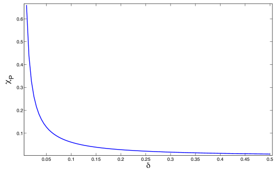
Figure 1: (Color online) Ratio between the electrostatic force at second order in the corrugation and the corresponding force at zeroth order ($\chi_{\rm P}=\frac{{\mathcal{F}}_{P,2}}{{\mathcal{F}}_{P,0}}$ ), as a function of the distance $\delta=d/R$, for the sphere-plane geometry. Parameters are: $p_{\rm max}R=10000$, $p_{\rm min}R=100$, and $\epsilon/R=0.001$.

We have numerically evaluated the effect of the roughness on the electrostatic force for the sphere-plane geometry, for the sharp-cutoff model. The result is shown in Fig.1, where the plot shows the ratio $\chi_{P}$ between the force at second order and the one at zeroth order in the corrugation. As expected, the effect of the roughness is more relevant at short distances. The plot shows a $1/d$ behaviour for small $d$, compatible with the previous analytic results for large values of $p_{\rm max}$.

V Results for the Casimir effect

V.1 Dirichlet boundary conditions

In the Dirichlet Casimir effect there is no dimensional parameter in the problem coming from the expansion of $F$, except from $a$. In particular, this means that both ${\widetilde{g}}^{(2)}$ and ${\widetilde{h}}^{(2)}$ are dimensionless functions of ${\mathbf{l}_{\shortparallel}}$.

We consider here the calculation of the function $V_{2}$, the effective potential term in the DE to the second order in the amplitude. To that end, we need the ${\widetilde{f}}^{(2)}$ kernel. This object has already been calculated Foscoetal2011 , and the result may be put as follows: ${\widetilde{f}}^{(2)}({\mathbf{k}}_{\shortparallel})=\big{[}{\widetilde{f}}^{(2)}(k_{\shortparallel})\big{]}\Big{|}_{k_{0}\to 0}$, where pfaT

$${\widetilde{f}}^{(2)}(k_{\shortparallel})\;=\;-2\int\frac{d^{3}p_{\shortparallel}}{(2\pi)^{3}}\;\frac{|p_{\shortparallel}|\,|p_{\shortparallel}+k_{\shortparallel}|}{(1-e^{-2a|p_{\shortparallel}|})(e^{2a|p_{\shortparallel}+k_{\shortparallel}|}-1)}$$ (77)

where we have used the notation $l_{\shortparallel}\equiv(l_{0},l_{1},l_{2})$, and $|l_{\shortparallel}|\equiv\sqrt{l_{0}^{2}+{\mathbf{l}_{\shortparallel}}^{2}}$, for any $3$-vector $l_{\shortparallel}$.

Thus, in this case, the function ${\widetilde{g}}^{(2)}({\mathbf{l}_{\shortparallel}})$ is a dimensionless function independent of any dimensionful parameter and, in practice, it may be obtained as follows:

$${\widetilde{g}}^{(2)}({\mathbf{l}_{\shortparallel}})\,=\,\big{[}{\widetilde{f}}^{(2)}({\mathbf{l}_{\shortparallel}})\big{]}\Big{|}_{a\to 1}\;,$$ (78)

which may be written explicitly as follows ($x$ = $|{\mathbf{l}_{\shortparallel}}|$):

$${\widetilde{g}}^{(2)}(x) = \frac{x^{3}\text{Li}_{2}\left(e^{-2x}\right)}{48\pi^{2}}+\frac{x^{2}\text{Li}_{3}\left(e^{-2x}\right)}{24\pi^{2}}+\frac{x\text{Li}_{4}\left(e^{-2x}\right)}{16\pi^{2}}+\frac{\text{Li}_{5}\left(e^{-2x}\right)}{16\pi^{2}}+\frac{\pi^{2}\text{Li}_{2}\left(1-e^{-2x}\right)}{240x}$$ (79)

$$+ \frac{\text{Li}_{6}\left(e^{-2x}\right)-\frac{\pi^{6}}{945}}{32\pi^{2}x}-\frac{x^{4}\log\left(1-e^{-2x}\right)}{120\pi^{2}}+\frac{\pi^{2}x}{240},$$

where ${\rm Li}_{n}(x)$ denote the Polylogarithm functions.

In Fig.2 we show the numerical evaluation of Eq.(43) for the Dirichlet Casimir energy for the sphere-plane geometry, using the sharp cutoff model for the roughness. In this figure we plot the ratio between the second and zeroth order in the corrugation $F_{P,2}/F_{P,0}$ as a function of the minimal distance between the sphere and the plane. The $1/d$ behaviour is similar to the one of the electrostatic case, and can be derived analytically for large values of $p_{\rm max}$ taking into account the large $x$ limit of ${\widetilde{g}}^{(2)}(x)$.

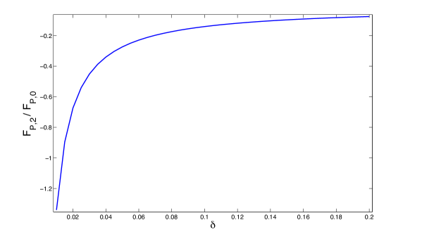
Figure 2: (Color online) Ratio between the Dirichlet Casimir energy at second in the corrugation, and zeroth order as a function of the distance $\delta=d/R$, for the sphere-plane geometry. Parameters are: $p_{\rm max}R=10000$, $p_{\rm min}R=100$, and $\epsilon/R=0.001$.

V.2 Neumann boundary conditions

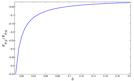
Figure 3: (Color online) Ratio between the Neumann Casimir energy at second and zeroth order in the corrugation as a function of the distance $\delta=d/R$, for the sphere-plane geometry. Parameters are: $p_{\rm max}R=10000$, $p_{\rm min}R=100$, and $\epsilon/R=0.001$.

In the Neumann Casimir effect, the function ${\widetilde{f}}^{(2)}$ is given by pfaT :

$${\widetilde{f}}^{(2)}(k_{\shortparallel})=-2\,\int\frac{d^{3}p_{\shortparallel}}{(2\pi)^{3}}\frac{\big{[}p_{\shortparallel}\cdot(p_{\shortparallel}+k_{\shortparallel})\big{]}^{2}}{|p_{\shortparallel}|\,|p_{\shortparallel}+k_{\shortparallel}|}\,\frac{1}{1-e^{-2a|p_{\shortparallel}|}}\frac{1}{e^{2a|p_{\shortparallel}+k_{\shortparallel}|}-1}\;.$$ (80)

and therefore

$${\widetilde{g}}^{(2)}(x)=-\frac{1}{24}\left(\frac{x^{2}}{2\pi^{2}}+1\right)x\text{Li}_{2}\left(e^{-2x}\right)+\left(\frac{x^{2}}{48\pi^{2}}-\frac{1}{16}\right)\text{Li}_{3}\left(e^{-2x}\right)$$ (81)

$$+ \frac{5x\text{Li}_{4}\left(e^{-2x}\right)}{32\pi^{2}}+\frac{7\text{Li}_{5}\left(e^{-2x}\right)}{32\pi^{2}}+\frac{\pi^{2}\text{Li}_{2}\left(1-e^{-2x}\right)}{240x}$$

$$+ \frac{-\pi^{2}\text{Li}_{4}\left(e^{-2x}\right)+\frac{7\text{Li}_{6}\left(e^{-2x}\right)}{2}+\frac{\pi^{6}}{135}}{32\pi^{2}x}-\frac{x^{4}\log\left(1-e^{-2x}\right)}{120\pi^{2}}+\frac{\pi^{2}x}{720}\,.$$

In Fig. 3 we show the numerical result of evaluating Eq.(43) for the Neumann Casimir energy for the sphere-plane geometry, using the sharp cutoff model for the roughness. Once again, the effect of the roughness becomes relevant at short distances.

VI Conclusions

We have found general expressions for the DE of the interaction energy between two surfaces, including the first nontrivial correction due to corrugation, assumed to exist on top of an otherwise smooth surface facing a plane.

The procedure we have followed to compute the interaction energy between surfaces is conceptually very simple. Due to the roughness, the functional that describes the interaction energy between surfaces does not admit an expansion in derivatives. However, after averaging over the small scale fluctuations, the resulting functional only depends on the shape of the smooth surfaces (the spatial averages of the rough ones), and therefore it makes sense to compute it using a DE. The leading order correction $F_{\rm P,2}$ can be thought as the usual PFA applied to the effective interaction that takes into account the roughness on parallel plates, while the next to leading term improves that by adding corrections depending on the derivatives of the function which defines the curved surface.

Note that, although the roughness is assumed to be described as a random variable, its statistical properties become inextricably mixed with the geometry of the surface, even at the first non-trivial order in the amplitude. At this order, the two-point correlation function is all the information that one needs to know. It should be clear that the general results could be applied the other way around, namely, one could attempt to determine the characteristics of the roughness of a surface by performing force measurements.

We have applied the general results to the case of the interaction between a rough sphere and a plane, both for electrostatic and Casimir interactions. We have considered the particular case in which roughness can be described by a simple correlation function which is constant between the bandwidth set up by two momentum space cutoffs. Of course the results can be extended to more realistic correlation functions, including roughness described by self-affine fractal scaling.

The results of this paper could also be generalized in other directions, like for instance to the case of two curved surfaces having roughness and finite conductivity.

References

- (1) B.V. Derjaguin, Koll. Z. 69, 155 (1934); B. V. Derjaguin and I. I. Abrikosova, Sov. Phys. JETP 3, 819 (1957); B. V. Derjaguin, Sci. Am. 203, 47 (1960); J. Blocki, J. Randrup, W.J. Swiatecki, and C.F. Tsang, Ann.Phys. (NY) 105, 427 (1977); J. Blocki and W.J. Swiatecki, Ann.Phys. (NY) 132, 53 (1981).
- (2) C. D. Fosco, F. C. Lombardo and F. D. Mazzitelli, Phys. Rev. D 84, 105031 (2011).
- (3) C. D. Fosco, F. C. Lombardo and F. D. Mazzitelli, Phys. Rev. D 89, 062120 (2014).
- (4) G. Bimonte, T. Emig, R.L. Jaffe and M. Kardar, EPL 97, 50001 (2012).
- (5) G. Bimonte, T. Emig, and M. Kardar, App. Phys. Lett. 100, 074110 (2012).
- (6) C. D. Fosco, F. C. Lombardo and F. D. Mazzitelli, Phys. Rev. D 85, 125037 (2012).
- (7) C. D. Fosco, F. C. Lombardo and F. D. Mazzitelli, Phys. Rev. D 85, 125037 (2012).
- (8) Y.P. Zhao, G.C. Wang, T.M. Lu, G. Palasantzas, G. and J. Th.M. De Hosson, Phys. Rev. B 60, 9157 (1999).
- (9) M. Bordag, G.L. Klimchitskaya, U. Mohideen, and V. M. Mostepanenko, Advances in the Casimir Effect, Oxford University Press, Oxford, 2009.
- (10) F. Intravaia et al, Nature Communications 4, 2515 (2013).
- (11) A.A. Banishev, J. Wagner, T. Emig, R. Zandi and U. Mohideen, Phys. Rev. Lett.110, 25043 (2013); ibidem arXiv:1402.2716.
- (12) H. Li and M. Kardar, Phys. Rev. Lett. 67, 3275 (1991).
- (13) P. A. Maia Neto, A. Lambrecht, and S. Reynaud, Phys. Rev. A 72, 012115 (2005); Erratum Phys. Rev. A 86, 059901 (2012).
- (14) H.Y. Wu and M. Schaden, Phys. Rev. D 89, 105003 (2014).
- (15) W. Broer, G. Palasantzas, J. Knoester, and V. B. Svetovoy, EPL 95, 30001 (2011).
- (16) M. Kruger,V. A. Golyk, G. Bimonte, and M. Kardar, EPL 104, 41001 (2013).
- (17) C. D. Fosco, F. C. Lombardo and F. D. Mazzitelli, Phys. Rev. D 86, 125018 (2012).
- (18) C. D. Fosco, F. C. Lombardo and F. D. Mazzitelli, Annals Phys. 327, 2050 (2012).