Molecular dynamics simulation: a tool for exploration and discovery using simple models

Abstract

Emergent phenomena share the fascinating property of not being obvious consequences of the design of the system in which they appear. This characteristic is no less relevant when attempting to simulate such phenomena, given that the outcome is not always a foregone conclusion. The present survey focuses on several simple model systems that exhibit surprisingly rich emergent behavior, all studied by molecular dynamics (MD) simulation. The examples are taken from the disparate fields of fluid dynamics, granular matter and supramolecular self-assembly. In studies of fluids modeled at the detailed microscopic level using discrete particles, the simulations demonstrate that complex hydrodynamic phenomena in rotating and convecting fluids – the Taylor–Couette and Rayleigh–Bénard instabilities – can not only be observed within the limited length and time scales accessible to MD, but even quantitative agreement can be achieved. Simulation of highly counterintuitive segregation phenomena in granular mixtures, again using MD methods, but now augmented by forces producing damping and friction, leads to results that resemble experimentally observed axial and radial segregation in the case of a rotating cylinder, and to a novel form of horizontal segregation in a vertically vibrated layer. Finally, when modeling self-assembly processes analogous to the formation of the polyhedral shells that package spherical viruses, simulation of suitably shaped particles reveals the ability to produce complete, error-free assembly, and leads to the important general observation that reversible growth steps contribute to the high yield. While there are limitations to the MD approach, both computational and conceptual, the results offer a tantalizing hint of the kinds of phenomena that can be explored, and what might be discovered when sufficient resources are brought to bear on a problem.

• 22 October 2014

Keywords: molecular dynamics simulation, emergent phenomena, atomistic hydrodynamics, granular segregation, molecular self-assembly, GPU computing

1 Introduction

The behavior associated with emergent phenomena is unusual in the sense that it is not an obvious consequence of the system design. ‘Emergence’, where the whole appears to be more than just the sum of its parts, is a term in widespread use, particularly in the biological and social sciences. However, when used to characterize effects that are inherently physical, the presence of some unknown component is not implied, but merely a manifestation of cooperative behavior that the theoretician’s tools are unable to deduce from the underlying equations. (There is a certain arbitrariness in designating phenomena as emergent, with the field of phase transitions often excluded, probably due to its theoretical foundations predating the popularization of the concept).

Computer simulation provides an ideal framework for studying physical phenomena that exhibit emergent characteristics. Simulation, unlike mere computation, aims to accommodate a more flexible outcome, thereby facilitating ‘exploration’; if the unexpected is encountered, this amounts to ‘discovery’. The discovery of emergent behavior in the course of a simulation is arguably even more surprising than in the real world, since the ingredients of the model system are (by definition) known, whereas in nature, as a last resort, emergence can always be attributed to mechanisms not fully understood.

The systems described in this article all exhibit emergent behavior. They are presented as a series of case studies and are based, for obvious reasons, on the author’s own work. The case studies, all involving classical molecular dynamics (MD) simulation, fall into distinct categories and are described in greater detail in subsequent sections of the paper; this grouping reflects the ability of emergence to manifest itself in different ways. The problems investigated can be summarized as follows: (a) Complex hydrodynamic behavior in atomistic fluids: the Taylor–Couette and Rayleigh–Bénard instabilities where structured flow patterns develop under the appropriate conditions. (b) Granular segregation: the components of a binary mixture of particles with different properties undergo axial and/or radial segregation in a rotating cylinder, or horizontal segregation in a layer placed on a vertically vibrated base with sawtooth grooves. (c) Supramolecular self-assembly: the spontaneous formation of polyhedral shells from particles of suitable shape, behavior analogous to the growth of protein shells that encapsulate spherical viruses.

Emergent behavior is associated with effects occurring at a ‘higher’ level than the participating elements. In the case of complex fluid flow, the atoms have little ‘awareness’ of collective movement on spatial and temporal scales far beyond the mean interatomic separation and the mean time between collisions. The same is true for segregating grains, although most will gradually become aware that they are surrounded by similar neighbors. With self-assembly, the molecular constituents are continually forming and breaking bonds, but gradually find themselves completely bonded, with little or no possibility of escape, as they are incorporated into the growing shells. In each of the examples, individual particles respond to the forces exerted by their immediate surroundings and, where relevant, boundary walls and an external force such as gravity; the common characteristic shared by these systems is that, if and when large-scale coherent behavior does emerge, it does so spontaneously.

Although the systems described here are mostly familiar, the a priori expectation of what simulations might be capable of achieving range from the uninteresting case of nothing, to the ideal outcome in which the rich complexity of the real world is reproduced. In studies of fluid flow, the surprise would be that macroscopic phenomena actually persist down to the microscopic scales accessible to MD. A successful outcome may show qualitatively meaningful behavior or even quantitative agreement with experiment and/or theory. Failure could reflect inadequacy of the model, unsuitable parameter choices, or simulations of systems that are too small to accommodate the range of length scales involved or run for insufficient time for the phenomena to develop. Resolution of the size and time limitations is aided to a modest extent by advances in computer performance. Spurious artifacts, implying behavior not observed in nature, are also a possibility. It goes without saying that mere reproduction of known behavior, no matter how complex, is not the ultimate goal; once a phenomenon has been captured ‘in silico’, questions can be asked concerning mechanisms that might be experimentally inaccessible, with a view to investigating the cooperativity ultimately responsible for emergent behavior.

Direct observation is crucial for the study of complex phenomena in the real world, the reason being that quantitative characterization is not always possible, and even when it is, the information supplied may be incapable of describing the intricate details. Computer visualization plays the corresponding role in the simulational environment. Actual observation of complicated and sometimes unexpected behavior arising in a simulation is also an illuminating experience because it reinforces the appreciation that complexity can have simple origins. The results included here emphasize the visual aspect, and are supplemented with limited quantitative details when theoretical or experimental comparison is possible or if the description of the phenomenon is enhanced by numerical data; further analysis is deferred to subsequent publications that focus on the individual systems.

The case studies are all based on new simulations that revisit problems considered in the past. The updated computations take advantage of recent advances in MD methodology enabled by GPU-based (GPU = graphic processing unit) computing that offer a 1–2 orders of magnitude performance improvement (depending on the type of computation and when the earlier work was carried out) to increase the system size and/or time covered. Larger systems can reduce finite-size effects, and in some instances, described later, the models themselves have been enhanced in various ways. The effect of these changes is reflected in the results. Improved computing power increases the scope for exploration; some of the examples considered here that originally required weeks of computing can now be completed in a single day, those needing months now complete in a week, while others of a less demanding (but still substantial) nature can now even be carried out interactively; the implications for proposed future study of these and related systems are obvious.

The organization of the paper is as follows. General aspects of MD simulation methodology are briefly summarized in Section 2, including model design and parameterization, algorithms and optimization for modern high-performance processors, inherent limitations of the MD approach due to the simplified models and heavy resource requirements, and the issue of reproducibility that arises when dealing with emergent behavior. The individual case studies are described in Sections 3–5: the background to each of the problems is covered, and the customized models and extensions to general MD procedures required for the simulations introduced, together with their limitations; the results accompanying the studies emphasize the more unexpected aspects of the behavior. Finally, Section 6 provides a retrospective outlook, attempting to strike a balance between the capabilities of the simulational approach and the rewards anticipated from the exploration of problems of increasing size and complexity.

2 Methods

Molecular dynamics simulation, or MD, a well-established approach conceived early in the computer age [1, 2], is aimed at probing the detailed dynamics of an extremely broad range of atomic and molecular systems, leading, among other notable accomplishments, to an understanding of liquid structure and dynamics, and helping gain a recent (2013) Nobel Prize for contributions to biomolecular dynamics. The methodology, e.g., [3], is based on classical dynamics, and while quantum theory often underlies the models, in particular the interaction potentials, explicit quantum effects are usually excluded. Simplified models are a key requirement to avoid being overwhelmed by excessive molecular detail; however, while it is essential to identify the important elements, it is not always obvious what assumptions are allowed. As with any theory, confirmation of whether the outcome of a simulation mirrors reality, either qualitatively or quantitatively, or is a mere artifice of the model, must come from outside the simulational framework.

While each of the case studies involves discrete particles and MD methodology, particles can represent different kinds of objects. For the fluid studies, unlike conventional computational and theoretical fluid dynamics that regard a fluid as a continuous medium, the MD approach adopts an atomistic viewpoint, using the simplest possible soft-sphere particles to represent the individual atoms or molecules; intrinsic properties of the fluid, such as the viscosity, thermal expansion coefficient and heat capacity, are determined by the system itself rather than specified as parameters. When modeling granular matter, the model particles correspond to grains; granular simulations generally consider spherical particles, using dissipative, velocity-dependent interactions as well as history-dependent interactions to emulate the complexities of friction, but in one of the current studies the particles consist of rigid tetrahedral arrays of soft spheres allowing the frictional forces to be simplified (partly for computational reasons). Finally, in the case of self-assembly, each protein capsomer (as the assembling particles are known) is again represented by a set of soft spheres arranged on a suitable rigid framework, with attractive forces acting selectively between interaction sites located on different particles to produce bonding; the particles themselves are immersed in a solvent consisting of soft-sphere atoms.

Each of the systems considered involves excluded-volume interactions between the soft spheres; there are additional interactions, treated in later sections, that are problem specific. Two versions of the soft-sphere interaction are used. For the fluid and self-assembly simulations, the force is based on the truncated Lennard-Jones potential

$$u_{s}(r)=4\epsilon\,[(\sigma/r)^{12}-(\sigma/r)^{6}]\qquad r<r_{c}$$ (1)

where $r=|{\bm{r}}|$ is the distance between particle centers; the cutoff range, $r_{c}=2^{1/6}\sigma$, ensures that the force is repulsive. In the granular simulations, the force depends linearly on particle overlap and is derived from the potential

$$u_{\ell}(r)=(k_{n}/2)\,(r_{c}-r)^{2}\qquad r<r_{c}$$ (2)

where $k_{n}$ is the force constant, and the cutoff range is determined by the mean diameter of the particles involved. In both cases the interactions ensure that the maximum particle overlap (which reflects the effective particle diameter and depends on the relative speed at impact and on local stresses) is minimal.

The use of reduced (dimensionless) MD units is implicit; though not required here, results expressed in reduced units are readily converted to physical units for comparison with experiment. For simulations of atoms or molecules, the reduced unit of length is expressed in terms of $\sigma$, which for argon is 3.4 Å (a typical value), and spheres have unit mass; the time unit is determined by $\epsilon$ and corresponds to $2.16\times 10^{-12}$ s (also for argon). Setting the Boltzmann constant to unity defines the temperature unit. For the granular simulations, length is defined in terms of the nominal particle diameter (if there is more than one species the smallest size is used), and to maintain consistency with earlier work $r_{c}$ is set to $2^{1/6}\times$ (mean diameter); the diameter is typically $10^{-3}$ m, and the time unit is then determined from the value of the gravitational acceleration $g$ so that the rotation or vibration rates correspond to experiment (described later). All the simulations use an integration timestep of 0.005 (MD units).

General MD methodology covers a variety of algorithms and computational tasks required by the simulations, including the organization of the force evaluations in a manner that scales linearly with the number of particles, the integration of the equations of motion for long simulations while ensuring stability, rigid-body dynamics, treatment of boundary conditions and the system initialization process, as well as details specific to individual problems including analysis techniques. These issues are addressed in [3], where the software required for many different types of MD simulations is described in detail. Additionally, the case studies described here use optimized MD software based on algorithms customized for GPU use [4] that, in some respects, differ significantly from their conventional counterparts. These GPU techniques have been extended to handle the specialized needs of the current work, including rigid bodies, various kinds of complex boundary conditions, multiple particle species, various force types and external fields, and have also been updated to utilize new hardware capabilities in the latest generation of GPUs not available for the earlier work (the actual GPU used here is the NVIDIA K20, whose massively parallel set of 2496 computational cores is fully utilized in the simulations).

Typically, relatively large systems and long runs are required to cover the multiple length and time scales intrinsic to each of the systems. A run must follow the entire evolution of the simulation, from its initial state until the expected (or unexpected) behavior has had the opportunity to develop and stabilize. Because local ‘knowledge’ must be allowed to propagate throughout the system, often a slow process that proceeds at diffusive rates, the length and time scales are sometimes coupled, so bigger systems may need to be simulated for longer time periods, further increasing the rate at which the computational burden increases with system size. The dynamics are driven entirely by deterministic interactions; the only stochastic element in the simulations is the set of random initial velocities (and also the particle species designation if multiple species are involved).

The particle trajectories themselves provide the raw data from which the results are derived, such as the flow and temperature fields that can be extracted by suitable coarse-grained averaging, the search for assembled structures by means of cluster analysis performed on particle configurations, or simple thermodynamic measurements. Depending on the problem, snapshots of either the particle positions or the flow fields are recorded over the course of each simulation, and subsequent quantitative analysis is based on these recorded summaries. Interactive visualization capabilities are incorporated into each of the simulations, allowing progress to be monitored, and also enabling subsequent replay of the recorded snapshot files.

Each model involves adjustable parameters, some of which are crucial to determining behavior, others less so. Certain parameters correspond directly to macroscopically measurable quantities, such as density, temperature or gravitational field, with some parameter combinations yielding dimensionless values such as the Reynolds or Rayleigh numbers, while other parameters are more closely associated with the model itself, such as the interaction strengths, the components of the friction forces, particle-wall interactions and particle shape. Each such parameter contributes to the overall behavior, either in the same manner as its macroscopic analog, if one exists, or possibly in a less obvious manner if it only appears in the definition of the model; consequently, even if the model is correctly designed in principle, emergent behavior might only manifest itself over limited parameter ranges. The relation between macroscopic quantities and model parameters is obvious in some cases, such as temperature which is proportional to mean kinetic energy, less obvious in others such as the Reynolds number which is useful only when the fluid viscosity does not vary significantly, an assumption not necessarily true under MD flow conditions, and difficult to resolve as in the case of macroscopic rate constants for self-assembly which, although dependent on interaction strength and concentration, can have as many distinct values as there are assembly steps.

An important issue bearing on simulations of complex behavior is reproducibility. This feature is no less vital in simulation than in experiment, and is not usually a problem, especially when simply measuring averages in a system already in a steady state. However, with simulations whose outcomes are ‘singular’ events (typically related to the emergent aspect of the behavior), and where computational cost limits sample coverage based on multiple runs with different initial conditions, it is not always possible to satisfy this requirement. In each such run, these events (here they would be associated with the stages of flow development, spatial segregation or cluster formation) can lead to changed final states, or can appear at different times, or sometimes even fail to appear at all. Moreover, a run started from a particular initial state may itself have limited reproducibility given that different computer hardware and software combinations can produce minute changes to floating-point results that grow exponentially with time, a well-known effect due to the underlying chaotic nature of MD trajectories, leading to altered collective behavior (the same is true in experiment, though for other reasons). Finally, with modern parallel computers (GPUs in particular), the computation order itself may be beyond user control (known as a race condition), leading to similarly irreproducible outcomes. However, if the system state is not too close to a phase transition (in the most general sense), the results can be expected to be similar, even if some of the less-important details vary.

3 Atomistic fluid dynamics

MD provides, at least in principle, a direct approach to the study of fluid dynamics and the variety of complex flows associated with hydrodynamic instability, such as those illustrated in [5]. Due to its heavy computational demands, MD cannot compete with well-established continuum techniques (nor with lattice-based methods), but it does offer a means for overcoming issues introduced when quantities commonly represented by continuous fields need to allow for features such as free surfaces, multiple components, and history-dependent behavior associated with complex rheology. On the other hand, given the restriction to relatively small systems over limited time intervals, there is the question of whether the familiar continuum behavior is relevant at all in MD work; only the simulations themselves are capable of providing an answer. An early step in bridging the conceptual gap between atomistic fluids and the continuum was an MD study of long-time effects arising from correlations in the atomic trajectories [6].

Much of conventional hydrodynamics is governed by dimensionless parameter combinations such as the Reynolds and Rayleigh numbers; in some cases MD allows systems to achieve the values needed to produce the associated laminar flow instabilities, but to compensate for the small size the conditions imposed, such as a high shear rate or temperature gradient, differ by orders of magnitude from the experimental regime. Even the transport coefficients can vary across the system (due to density and temperature variations), unlike experiment where they are typically regarded as constant (as in Newtonian fluids). Care is needed to avoid artifacts due to these extreme conditions. An additional complication for MD is the need to counteract viscous heating and maintain nonslip boundaries, all without adversely affecting the phenomena under study.

In view of these complicating factors, the expected outcome of an MD-based fluid simulation ranges from nothing interesting if the system is too small or the times scales inaccessible, transient effects if flows cannot be sustained because of inadequate contact with the boundaries or coupling to the driving field (resulting in an inability to establish nonslip flow or an appropriate temperature gradient), and totally unrelated behavior if the conditions are too extreme. Given the many possible failure modes, the appearance of behavior that is qualitatively, and even quantitatively correct, offers a pleasant surprise.

The initial applications of MD to questions of hydrodynamic instability focused on phenomena for which a less computationally demanding two-dimensional version could be studied, in particular, the vortices that form in flow past a bluff body [7, 8] and Rayleigh–Bénard convection [9, 10, 11, 12, 13]. The two systems discussed here are three-dimensional: Taylor–Couette flow that only exists in three dimensions, and the more realistic three-dimensional version of the Rayleigh–Bénard problem [14]. Other examples for which the MD approach has proved successful include the Rayleigh–Taylor phenomenon [15] and droplet formation during the breakup of fluid jets [16]. In all applications of MD to hydrodynamics, fluid flow is superimposed on the thermal motion of the atoms, the latter entirely absent from the continuum representation; there is a further difference between the two problems considered here, namely that vortex flow in the Taylor–Couette system, itself a consequence of the instability caused by an adverse angular momentum gradient, is superimposed on the overall azimuthal flow, while in the Rayleigh–Bénard system, where the instability is due to an adverse temperature gradient, convection is the only flow present.

3.1 Taylor–Couette vortices

The formation of toroidal vortices in a fluid confined to an annular gap between concentric rotating cylinders, known as the Taylor–Couette phenomenon [17, 14, 18], is arguably the most thoroughly studied of hydrodynamic instabilities. Consider the experimental cell defined in Figure 1, where $d=r_{o}-r_{i}$ is the width of the annulus. For the case of a stationary outer cylinder and an inner cylinder rotating with angular velocity $\omega$, the flow depends on the dimensionless Taylor number

$$Ta=4[(r_{o}-r_{i})/(r_{o}+r_{i})]\,Re^{2}$$ (3)

where

$$Re=dr_{i}\omega/\nu$$ (4)

is the Reynolds number and $\nu$ the kinematic viscosity. The flow is purely azimuthal at low $Ta$, but at a critical $Ta_{c}$, whose value can be computed from a stability analysis of the Navier-Stokes equations [14], secondary flow patterns appear that have the form of regularly spaced axisymmetric vortices. The wavelength of this pattern, corresponding to the axial length of a pair of counter-rotating vortices, is close to $2d$. At higher $Ta$ [19, 20, 21] additional azimuthal wave instabilities appear and eventually turbulence. Numerical results using the conventional continuum approach are described in [22, 23]. Experimental studies have employed a variety of measurement techniques in examining different aspects of the flow; examples include [24, 25, 26, 27, 28, 29].

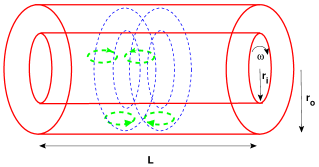
Figure 1: Schematic diagram of the Taylor–Couette cell in which the fluid is confined to the annular region and the inner cylinder rotates; counter-rotating vortex rolls (such as those shown) are superimposed on the overall azimuthal flow.

Several additions to the standard MD approach are needed to formulate an atomistic simulation of the Taylor–Couette system. The atoms themselves are soft spheres whose interactions are defined in (1). The sheared flow is driven by the curved cylinder walls which act both as nonslip boundaries and as thermal sinks for dissipating the heat produced by the shear [30]. The walls themselves are smooth; the mechanism for achieving an effective nonslip condition is that when an atom reaches the wall it bounces back with a new velocity whose direction is randomly chosen to be either reflection or reversal (the choice is actually deterministic, but there is a sensitive dependence on the impact position that yields a seemingly random outcome), and whose magnitude is fixed to achieve the desired temperature; at the inner wall the rotation velocity is added. The end caps of the region reflect atoms elastically. The computational effort is reduced by considering only a single quadrant of the annular region, with customized periodic boundaries, in which both coordinate and velocity vectors are suitably transformed, used to account for the remainder of the system during the force computations.

Flow studies require coarse-grained averaging to filter out thermal fluctuations and produce snapshots of the spatially varying flow field. The simulation region is subdivided into a grid of cells and the average properties, namely the velocity vector components, velocity magnitude and cell occupancy, evaluated for each cell over a short time interval. The degree of coarse-graining, namely the cell dimensions and the averaging interval, is determined by the conflicting demands of resolving the fine spatial and temporal details of varying flow patterns while suppressing the effect of local fluctuations. The resulting cell-averaged flow magnitude and direction, temperature and density retain no details of the actual particles from which they are derived, and in this respect their information content is equivalent to the continuum fluid description.

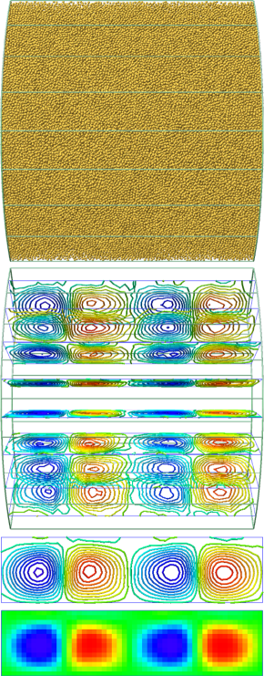
Figure 2: Alternative views of the smaller of the simulated Taylor–Couette systems (after 10 revolutions): a view of the atoms filling the annular quadrant (without the walls), streamlines based on the axial and radial flow components in several planes at different azimuthal angles, with color indicating the direction and speed of roll rotation, the same streamlines averaged azimuthally, and the corresponding color plot.

Earlier work demonstrated the ability of MD simulation to not only reproduce the Taylor–Couette vortices in a quantitatively correct fashion [30], but also the rate at which these secondary flow structures appear as a function of $\omega$ (or $Ta$) [31], allowing a detailed comparison between experiment, theory and simulation. Figure 2 shows several alternative views of a relatively small system, similar to that considered in [30], with $r_{i}=50$, $d=25$, $L=100$, containing $N\approx 1.2\times 10^{5}$ atoms, for $\omega=0.1$; $Ta\approx 1.6Ta_{c}$ for this system. The first of the views shows the actual MD system; the azimuthal component of the flow can be seen when the simulation is run interactively, superimposed on the thermal motion of the particles, but the fact that the averaged particle trajectories are helical, a consequence of the toroidal rolls, can only be inferred from the coarse-grained flow analysis. The next view shows the flow streamlines for several axial slices, after removing the azimuthal flow component; the vortex structure is now apparent, with color used to distinguish between counter-rotating flows. Since the final state is azimuthally symmetric (this is not true during early vortex development), full azimuthal averaging for further noise reduction leads to the streamlines in the next image, and finally the same information in a simplified, color-coded form (used later). These alternative views also exemplify the different kinds of information that appear as the level of representation is changed, ranging from excessively detailed particle motion to the spatially averaged flow of the continuum fluid, additionally simplified by symmetry.

The value of $d$ used in [30] is practically the smallest permitting vortex development. Larger systems are clearly desirable to reduce finite-size effects; increasing the annular width $d$ provides more room for roll growth, and if $L/d$ is also enlarged additional rolls can be accommodated. Recall, however, that even the biggest systems addressable by MD remain extremely microscopic. The system described here has $r_{i}=100$, $d=40$, $L=640$, providing a 20-fold size increase to $N\approx 2.35\times 10^{6}$. The extreme conditions to which the fluid is subjected, the shear rate being the most prominent, are alleviated slightly by reducing $\omega$ to 0.04. Overall, these changes increase $Ta$ by a factor of 1.4 and provide a fourfold increase in $L/d$.

The toroidal vortex evolution in this larger system over a run of $1.9\times 10^{7}$ timesteps, amounting to 650 revolutions, is shown in Figure 3. Rapid initial vortex formation appears within just four revolutions, covered by the first three frames of the sequence, followed by vortex merging and the disappearance of an adjacent pair of vortices after about ten revolutions in the next two frames. The last two frames show gradual vortex resizing leading to a final state that exhibits apparent long-term stability. Pattern development is not necessarily reproducible between runs, and where the final state consists of a sufficiently high number of vortices, even the existence of a preferred wavelength cannot fully constrain the number of vortices present in the final state; indeed, here there are 20 vortices, instead of 16 expected from the theoretical pattern wavelength. Extra vortices, both transient and permanent, are sometimes observed in the smaller system as well [31]; analogous effects are also encountered experimentally [32].

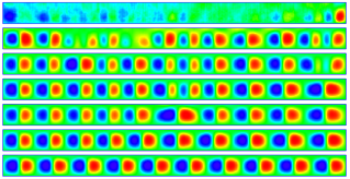
Figure 3: Azimuthally averaged color plots for the larger Taylor–Couette system at different times (after 1.4, 2.7, 4, 9, 10, 40 and 650 revolutions) showing the onset of the rolls and their subsequent merging and repositioning.

The radial component of the flow (azimuthally averaged) at the end of the run of the larger system is shown in Figure 4. Each of the 10 peaks along the cylinder axis corresponds to a vortex pair, with the outward flow faster than the inward; for the small system there are just two peaks, and [30] shows that even though the behavior is strongly nonsinusoidal, it can be fit to a three-term Fourier expansion with coefficients predicted by theory [21, 33]. The maximum radial velocity $\approx 0.4$, much smaller than the innermost value of the coarse-grained azimuthal flow, measured to be 3.8 ($\approx r_{i}\omega=4$); the 10-fold difference explains why rolls cannot be observed directly without averaging.

Figure 4: Axial dependence of the radial component of the flow velocity at the end of the Taylor–Couette simulation; each peak corresponds to a vortex pair.

3.2 Rayleigh–Bénard convection cells

The Rayleigh–Bénard phenomenon – the rich variety of flow patterns produced by convection in a fluid layer heated from below – is another well-known example of hydrodynamic instability [14, 34, 18, 35, 36, 37]. The system is defined in Figure 5, and its behavior is governed principally (but not entirely) by the dimensionless Rayleigh number

$$Ra=\alpha gL_{z}^{3}\Delta T/\nu\kappa$$ (5)

where $\alpha$ is the thermal expansion coefficient, $g$ the gravitational acceleration, $\Delta T=T_{hot}-T_{cold}$ the temperature difference, $\nu$ the kinematic viscosity, and $\kappa$ the thermal diffusivity (the other relevant ratio, not discussed here, is the Prandtl number $Pr=\nu/\kappa$). A critical value $Ra_{c}$ marks the onset of convection, where buoyancy overcomes viscous drag, and convection replaces conduction as the principal mechanism for thermal transport. Theory is simplified by the Boussinesq approximation, in which it is assumed that density is the only temperature-dependent fluid property; $Ra_{c}$ can then be computed for various kinds of boundary conditions [14], as can the wavelength of the convection pattern at criticality, but not the predicted planform, such as linear or concentric rolls, spirals, and hexagonal cells. The actual convection roll (or cell) width, typically of order $L_{z}$, represents a compromise: narrow rolls reduce shear losses at the nonslip walls, while wide rolls reduce viscous drag and diffusive heat transfer between oppositely moving hot and cold streams. The continuum version of the problem has been studied computationally, e.g., [38, 39, 40].

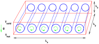
Figure 5: Schematic diagram of the Rayleigh–Bénard system; linear convection rolls are shown for illustrative purposes.

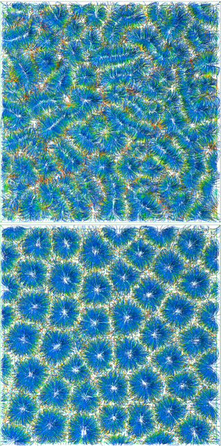
Figure 6: Streamlines from the larger Rayleigh–Bénard simulation early in the run where organized flow structures start to develop, and at the end of the run where there is a well-developed convection cell array.

In order to simulate the Rayleigh–Bénard system at the atomistic level the standard MD approach must be augmented by a mechanism for heat injection at the bottom wall and removal at the top, as well as a gravitational field. Coarse-grained flow analysis is once again required to examine the developing flow. The simulations described in [41] deal with a system of $N\approx 3\times 10^{6}$ atoms, together with an additional $\approx 0.5\times 10^{6}$ fixed atoms that form the bottom and top walls. A run of $3.2\times 10^{6}$ timesteps (of size 0.004), with $T_{hot}=10$, $T_{cold}=1$, and $g$ arbitrarily set to $3\Delta T/2L_{z}$ (a choice ensuring equality of the potential and kinetic energy changes across the layer), resulted in a periodic array of eight hexagonal convection cells. A narrower system with smaller $L_{y}$ produced linear rolls of the type shown schematically in Figure 5.

The system considered here has three times the number of atoms, with region size $L_{x}=L_{y}=679$ and $L_{z}=54.3$ (compared with the earlier $L_{x}=521$, $L_{y}=451$ and $L_{z}=35.3$ [41]), and $N=10^{7}$. $T_{hot}$ is lowered to 8 (for a less ‘extreme’ thermal gradient) and $g$ is halved to reduce density variation across the layer. These changes increase the nominal value of $Ra$ by 10%; since $Ra$ depends on $\nu$ and $\kappa$, both of which vary with local temperature and density, the actual value of $Ra$ is not readily determined (even its relevance under the extreme non-Boussinesq conditions is questionable). While the lateral boundaries are periodic as before, the bottom and top thermal walls are implemented using a new mechanism, avoiding the need for additional fixed atoms: Fluid atoms colliding with these horizontal, planar walls are assigned new velocities, with a magnitude set by the nominal wall temperature and direction corresponding to a random choice between reflection or reversal (the choice actually depends on the impact position, as in the Taylor–Couette simulations); in addition (following [41]), the velocities of all atoms close to the thermal walls (within $\approx r_{c}$) are rescaled at regular intervals, after zeroing their transverse average, to avoid any buildup of unwanted drift and help enforce the desired boundary temperatures. This change, as will become apparent from the results, leads to the development of narrower convection cells than before, in closer agreement with the expected behavior.

The outcome of the simulation after $10^{7}$ timesteps, requiring an order of magnitude more computation than previously, is a much more elaborate convection cell pattern. Streamlines are used in Figure 6 to show the nascent flow state after just $4\times 10^{4}$ timesteps, and the reasonably well-ordered cell array at its end. The color-coded streamlines show temperature variation, and while the downward flow of cold fluid at the cell centers is clearly visible when viewed from above, the upward flow of hot fluid at the cell edges is best seen when the system is viewed obliquely or from below (not shown). The measured vertical component of the flow velocity is in the approximate range (-1.8, 2.6), where the nominal thermal velocities are $\approx 1.7$ and 5 at the cold and hot boundaries respectively; at mid-height the velocity range is reduced to (-1.0, 2.0).

The early convection pattern contains certain linear features, but conversion into compact cells is complete after $\approx 3\times 10^{5}$ timesteps, following which there is a slow process of cell resizing and rearrangement; a series of snapshots showing how the cell pattern changes with time appears in Figure 7. Cell organization changes gradually, with no clear indication that the process eventually terminates; while the number of convection cells is almost constant (see Figure 8 below), new cells are seen to appear and existing cells merge, with each such event followed by rearrangement of nearby cells. It is worth bearing in mind that each convection cell represents coherent flow involving $\approx 2\times 10^{5}$ MD fluid atoms superimposed on the random thermal motion, an impressive exhibition of emergent collective behavior.

Quantitative cell analysis is based on coarse-grained temperature measurements at a height $0.3L_{z}$ above the hot bottom wall, where the variation is most pronounced. The cell centers are positioned at each of the local temperature minima (coincident with the downward flow maxima) and Voronoi polygon analysis (a simplified two-dimensional version of the technique described in [3], in which the plane is subdivided into polygons where the region nearer to a particular center than to any other is assigned to its polygon) is used to predict the cell boundaries. For a well-developed cell array these computed boundaries closely track the actual flow cell structure.

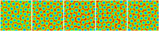
Figure 7: Variation of the convection cell pattern with time (larger Rayleigh–Bénard system, at times 0.7, 1.7, 2.7, 3.7 and $5\times 10^{4}$), with automated Voronoi analysis used to delineate cell boundaries.

A variety of measurements can be made based on the Voronoi polygon analysis. The convection cell count is shown as a function of time in Figure 8; the number of cells varies, but only over a narrow range. The average number of edges per polygon must of course be six, with an observed $\pm 1$ variation, the mean radius (specifically the mean inradius or distance from the polygon center to its edges) depends on the number of polygons and varies between 54 and 57, with a spread (a measure of the deviation from a regular polygon in which all distances are equal) that ranges from 2.3 to 12 for individual snapshots. The average value (and standard deviation) of this radial range is included in Figure 8, and the fact that it amounts to only about 10% of the mean radius is consistent with the observed regularity of the cell shapes. The underlying wavelength of the cell array, $\lambda$, is twice the mean radius, so that here the measured value of $\lambda/2$ is very close to $L_{z}$ (= 54.3).

Figure 8: Number of convection cells and their average radial range over the entire run (larger system).

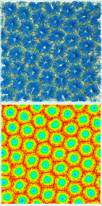
Figure 9: Flow streamlines and Voronoi analysis for the smaller Rayleigh–Bénard system showing the defect-free lattice of hexagonal convection cells.

There are considerably more convection cells in this simulation than in [41], a far larger number than can be attributed to the altered system size; in the earlier simulations $\lambda=5.27L_{z}$, but here this has dropped to $\lambda=2L_{z}$. Theory [14] predicts different $\lambda$ values for hexagonal cells and linear rolls, with $\lambda_{hex}/\lambda_{lin}=2.14$ and $\lambda_{lin}=2.016L_{z}$; different ratios for (gently curved) rolls and hexagons have been reported experimentally [42, 43, 44], even down to unity. Thus the fact that the MD hexagons have a value of $\lambda$ predicted for linear rolls is not unreasonable since experiment implies that the simplified theory is inadequate. The likely cause of the enlarged $\lambda$ in the earlier simulations is the wall implementation, where relying on collisions with a boundary array of spheres to produce the nonslip condition is less effective than individually adjusting the post-collision velocities; the present smaller $\lambda$, a value consistent with experiment, appears to be a consequence of the more effective method.

The dependence of $\lambda$ on $L_{z}$ is confirmed by considering a smaller but otherwise similar system. The size is reduced to $L_{x}=L_{y}=543$, $L_{z}=40.7$ (this $L_{z}$ is only slightly bigger than in [41]) and $N=4.8\times 10^{6}$; the edge ratios $L_{x}/L_{y}$ and $L_{x}/L_{z}$ are changed and the nominal $Ra$ is reduced by a factor of 0.4. The outcome of this run after $1.3\times 10^{7}$ timesteps, seen in Figure 9, is a perfect array of hexagonal convection cells; there is no visible change in this array over the last $3\times 10^{6}$ timesteps. From a Voronoi analysis of this run the mean polygon radius is 42.8, again very close to $L_{z}$, and the mean radial range of the cells is just 2% of the radius, confirming the observed regularity of the hexagon array. The initial orientation of the cells is decided spontaneously in the absence of physical lateral boundaries, although if the final state is a perfect array the periodic boundaries will constrain its orientation; multiple runs (with different initial conditions) show similar overall behavior but the detailed cell development differs. These represent initial results for this problem; the extended cell arrays ought to be amenable to Fourier analysis, not attempted for the very limited cell array in [41]. Furthermore, in view of the dependence on region size, shape and other parameters, as well as the sensitivity to the initial state originally seen in two dimensions [12], more extensive simulations, especially near the convection threshold [13], are likely to prove interesting.

4 Granular segregation

Granular dynamics is a field fraught with surprise, where the mechanisms responsible for much of the counterintuitive behavior remain a longstanding theoretical challenge; potential economic benefits provide ample motivation for achieving a systematic understanding of the phenomena involved. Since the behavior often differs strongly from systems explainable by fluid dynamics and statistical mechanics, established theory is limited in the help it can provide and, consequently, progress [45, 46, 47, 48] relies heavily on computer simulation.

Granular segregation is a fascinating example of emergent behavior: the ability of dry, noncohesive particle mixtures to separate into individual species, despite the absence of any obvious energetic or entropic advantage. Segregation and mixing are central to many kinds of industrial processing, so that the capability of either causing or preventing species separation is important.

Computational methods analogous to MD, with particles now corresponding to macroscopic grains, provide a flexible approach to simulating granular matter [49, 50, 51]. Additional forces are introduced to represent the effects of inelasticity and friction, the simplest of which is velocity-dependent collision damping; although the approximations tend to be empirical, since a full prescription for reproducing specific granular properties is unknown, suitable interaction functions allow simple spherical particles to mimic rough, irregular grains (in a vacuum). More complex particle shapes can also be employed, as is the case in one of the examples discussed here. Finally, since container boundaries are usually involved, often providing the driving force, the simulations must take them into account.

Granular simulations can have several possible outcomes, as was the case with atomistic fluid dynamics. These range from nothing interesting if the model fails to incorporate the essential properties of the granular medium, incorrect (but perhaps still interesting) behavior if the model somehow misrepresents reality, partially correct behavior in which some features are captured, and preferably, a correct reproduction of the form and sequence of the segregation process. With this in mind, two examples are described. One is a granular mixture in a horizontal rotating cylinder, a system known to exhibit various combinations of axial and radial size segregation; here, simulation successfully imitates experiment. The other is a mixed granular layer on a vertically vibrating, sawtooth-shaped base, where a combination of stratified horizontal counterflows and vertical (Brazil nut) size segregation might be expected to produce horizontal segregation; while the simulations support this prediction, experimental verification is still awaited.

4.1 Segregation in a rotating cylinder

Segregation of a binary mixture in a partially filled cylinder rotating around a horizontal axis is an extensively studied phenomenon [52]. Axial segregation is the most prominent effect, where a pattern of bands of alternating particle species develops along the axial direction; bands can gradually merge, at a rate that drops to such a low level that it is unknown whether the state eventually reached is stable, or just longlived. A second form of segregation, requiring greater effort to observe, occurs in the radial direction, resulting in a core rich in small particles surrounded by a layer of predominantly big particles; the radial core itself can be the final state, a transient state preceding axial segregation, or a feature which persists even when axial segregation is apparent externally.

Early experimental efforts involved direct observation of axial band structure from the outside [53]; some of the subsequent studies succeeded in examining the interior using MRI [54, 55] and relating the development of the axial bands to bulges occurring in the radial core. Time-dependent behavior can occur after the initial appearance of the axial bands, with gradual merging of narrower bands [56] and traveling surface waves [57]. Complicating the behavior are results showing that the ratio of cylinder to particle diameter determines if axial segregation is possible and whether its appearance depends reversibly on rotation rate [58]. Later experiments [59, 60] revealed more about the richness of the segregation effect and the associated dynamics under wet conditions; these are relevant because slurries tend to share the behavior of dry mixtures. Overall, no consensus has yet emerged as to the mechanisms underlying this form of segregation; the difficulties inherent in understanding granular matter are discussed in [47, 48, 61].

Granular simulations have proved capable of reproducing both the axial and radial forms of segregation. In [62] it was shown how the appearance of radial segregation precedes axial segregation, and that depending on the circumstances, a radial core of small particles could persist even after the external view showed essentially complete axial segregation. Corresponding behavior in three-component mixtures was described in [63]. Owing to the need for relatively large systems and long runs, only a very limited set of parameter combinations could be considered. The problem of following the development of segregation in detail is further exacerbated by a lack of reproducibility between runs that differ only in their initial states (i.e., the random initial velocities assigned to the particles) leading to varied segregation scenarios; the same is true experimentally, implying that multiple simulation runs are needed for observing typical behavior, a situation similar to the fluid studies discussed earlier.

Increased computer performance allows this problem to be revisited, but with several changes to the model. In [62] soft-sphere particles were used, together with the usual velocity-dependent normal and tangential forces for representing collision damping and sliding friction, defined in (6) and (7) below, as well as tangential restoring forces (involving the position histories of the relevant particle pairs) introduced to mimic the effect of static friction. In the new simulations, instead of using simple spherical particles, each particle is constructed from a set of spheres rigidly positioned on a (virtual) tetrahedral frame, as shown in Figure 10; particles of different size differ only in their tetrahedral arm lengths, in this case 0.6 and 1.2 (MD units). Unlike purely convex particles, the more complex effective shape allows particles to interlock, thereby partially reproducing the effect of static friction without the tangential restoring force used previously (whose GPU implementation is inconvenient); the geometrical interlocking effect is a simplified version of what really happens, where interlocking (and breakage) of multiple asperities on rough grain surfaces is the ultimate cause of static friction. The curved cylinder boundary is also required to emulate the effects of static friction, and this is achieved by embedding spherical particles in the surface of the rotating wall, arranged on a staggered grid with spacing 2.2, producing a sufficiently rough boundary to impede sliding. The cylinder end caps provide normal damping, but are otherwise smooth. The resulting segregation effects turn out to be unaffected by the alterations to the model.

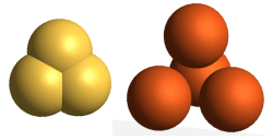
Figure 10: Particles used in the cylinder granular segregation simulations; each consists of four spheres in a rigid tetrahedral array (the virtual ‘framework’ is not shown), the only difference between big and small particles is the distance between spheres.

The particle interactions are based on [62], with the exception of the omitted tangential restoring force. The repulsive force between spheres ${\bm{f}}_{\ell}$ is obtained from the potential in (2), with $k_{n}=1000$. The velocity-dependent normal damping is

$${\bm{f}}_{d}=-\gamma_{n}({\hat{\bm{r}}}\cdot{\bm{v}}){\hat{\bm{r}}}$$ (6)

where ${\bm{v}}$ is the relative sphere velocity and $\gamma_{n}=5$. Sliding friction is due to tangential damping between particles within contact range

$${\bm{f}}_{s}=-\min(\gamma_{s}|{\bm{v}}_{t}|,\mu|{\bm{f}}_{\ell}+{\bm{f}}_{d}|){\hat{\bm{v}}}_{t}$$ (7)

where ${\bm{v}}_{t}$ is the transverse component of ${\bm{v}}$; the damping coefficients are $\gamma_{s}=10$ for spheres associated with the big particles and for sphere-wall contacts, and $\gamma_{s}=2$ otherwise (following [62], $\gamma_{s}$ is larger for big particles); the static friction coefficient $\mu\propto\gamma_{s}$, with a maximum of 0.5. Gravity is of course present.

The two examples considered here have different cylinder dimensions and demonstrate dissimilar segregation scenarios. One involves a shorter cylinder of length $L=200$ and diameter $D=100$, the other a longer cylinder with $L=500$ and $D=80$; the dimensions need to be larger than in [62] because of the increased effective particle size. For the initial state, particles are placed on a lattice filling the cylinder, assigned small random velocities, and the species (big or small) is set randomly; the lattice spacing is chosen to produce a specific fill level when particles settle on the bottom (the different fill levels can be seen in the pictures below) and in the present simulations the shorter cylinder is filled to a higher level. The fraction of big particles is 0.33; this ensures that when axial bands form, the total band widths for the two species are roughly equal. The number of particles in the two systems are $N=1.36\times 10^{5}$ and $1.03\times 10^{5}$; the actual number of soft spheres involved in the force computations (apart from the wall spheres) is four times larger. The cylinder rotates with angular velocity $\omega=0.2$; an upper bound to $\omega$ is set by the ratio of angular to gravitational acceleration, the Froude number $Fr=D\omega^{2}/2g$, to prevent particles forming a ringlike layer adjacent to the curved cylinder wall; here $g=5$, so $Fr=0.4$ and 0.32 for the two systems. If the length unit (the sphere diameter) is $10^{-3}$ m, then the time unit for this value of $g$ corresponds to 0.022 s, resulting in an experimentally reasonable 1.4 Hz rotation rate.

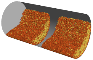
Figure 11: Radial granular segregation (shorter cylinder) with big and small particles colored red and yellow respectively; a slice has been removed to show the interior, and particles embedded in the curved cylinder wall (to produce surface roughness) are omitted.

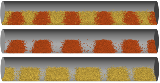
Figure 12: Axial granular segregation (longer cylinder); the complete system is shown, together with separate views of the big and small particles.

Simulation of the system with the shorter cylinder provides a demonstration of radial segregation, as shown in Figure 11. In this picture, a slice has been removed so that the interior organization (away from the end walls) can be seen; the inner core is dominated by small particles, and the majority of big particles reside in the outer layer. The onset of segregation is rapid, reaching completion after approximately 30 revolutions; radial segregation is also a fast process experimentally. The simulation run extends over a total of 1120 revolutions ($7.2\times 10^{6}$ timesteps) but no subsequent organizational changes are observed, a strong indication that this state is stable. The same system run at a reduced $\omega=0.1$ (not shown) produces even stronger radial segregation.

Simulation of the longer cylinder leads to an entirely different mode of behavior. The state after 1550 revolutions ($10^{7}$ timesteps) is shown in Figure 12; axial segregation is complete, with relatively few particles appearing outside their segregation bands, as is apparent from the views showing the individual species. During the early phase of the run the system exhibits transient radial segregation, and the space-time plots in Figure 13 show how radial and axial segregation appear in succession; only the first 500 revolutions are covered since no change occurs during the subsequent $>1000$ revolutions. Radial segregation appears rapidly, as before, but gradually fades after about 100 revolutions, when axial segregation begins to develop. Once the axial segregation process ends, there is very little particle transfer between bands (as might be deduced from Figure 12), exactly as in [62].

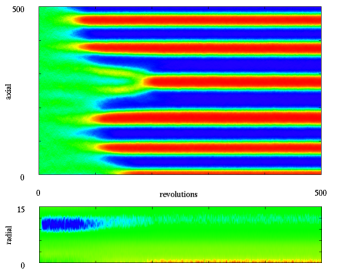
Figure 13: Space-time plots showing axial and radial populations (longer cylinder); the vertical axis corresponds to the axial or radial coordinates; red and blue represent regions of predominantly big and small particles, while other colors indicate mixed states.

4.2 Segregation in a vibrated layer

Another instance of unusual behavior associated with granular matter involves a vertically vibrated layer on a base whose surface is shaped as a series of asymmetric sawtooth grooves. Horizontal flow is observed [64], both experimentally, where the grains are confined to a narrow annular region between two upright cylinders, and in the corresponding simulations [65]. Moreover, the overall flow magnitude and direction depend on the parameters defining the system, such as the vibration frequency and amplitude, the sawtooth shape and the layer thickness, in a seemingly unpredictable manner. The simulations reveal that the induced flow rate actually varies with height within the layer; even more unexpected is the observation that oppositely directed flows at different heights can coexist, with flow close to the base directed up the less steep side of the teeth. Once it is realized that the horizontal flow is stratified in this fashion, the sensitive parameter dependence of the overall flow is seen to be a direct consequence of the competition between opposing flows.

A combination of the stratified flow with another phenomenon unique to granular matter, namely the familiar vertical size segregation under vibration, or ‘Brazil nut’ effect [66, 67], leads to the prediction of an entirely new kind of size-dependent segregation: Given that under suitable conditions the upper and lower parts of the layer flow horizontally in opposite directions when the sawtooth base is vibrated vertically, and that these same vibrations cause vertical size segregation within the layer, then it is reasonable to expect that a granular mixture will undergo horizontal size segregation on a vertically vibrating sawtooth base. Simulations [68] have demonstrated that this effect actually occurs, at least in the computer.

Two examples of three-dimensional systems are considered, one a rectangular box with linear sawtooth grooves, the other a cylindrical container with concentric circular grooves; in [68] the two-dimensional version of the box was considered, and the cylinder mentioned only briefly. The granular model used here is simpler than for the rotating cylinder. The grains are represented by soft spheres whose sizes are narrowly distributed about two distinct mean values. The interactions between particles include just the overlap repulsion (2) and normal damping (6), without the tangential component. Each sawtooth is formed from several closely spaced, narrow, linear or ringlike cylinders, horizontally and vertically positioned to approximate the profile; granular particles near the sawtooth base interact with one or more of these cylinders, with overlap repulsion and damping acting in the plane normal to the (local) cylinder direction. Gravity is present, and the vertical container walls are smooth.

The horizontal dimensions of the rectangular box are $270\times 135$ while the cylinder has a diameter of 270; in both cases the containers are sufficiently high for the upper boundary to be beyond the range of particle motion, and both contain $2\times 10^{5}$ particles. The small particles have unit maximum diameter, the big particles 1.5, with a small random value ($<0.1$) subtracted to suppress any tendency to order; the fraction of big particles is 0.3. The vibration frequency is $f=0.4$, the amplitude $a=1$, and $g=5$; conversion to physical units is as before, resulting in a frequency of 18 Hz. The ratio of vibrational to gravitational acceleration, $\Gamma=(2\pi f)^{2}a/g$, is a quantity relevant to the behavior of vibrating layers, with a minimum $\Gamma\approx 1$ required to excite the layer, and too large a value producing surface waves and eventually layer breakup; here $\Gamma=1.26$. Each gradually sloping sawtooth edge is of approximate length 13, while the steep edge is practically vertical; the sawtooth dimensions influence the effectiveness and even the direction of the segregation process [68].

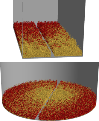
Figure 14: Horizontal segregation in vertically vibrated granular layers with a sawtooth base; slices have been removed to shown the interior.

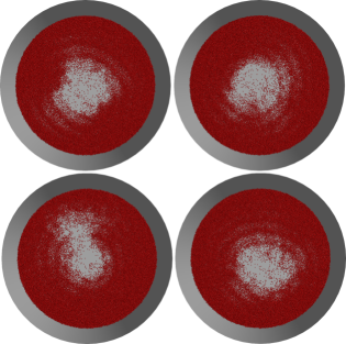
Figure 15: Segregated big particles (viewed from above) at intervals of 1200 vibration cycles.

The outcome of the simulations of the two systems is shown in Figure 14, the box after $9\times 10^{4}$ vibration cycles, the cylinder after $4\times 10^{4}$ cycles. Segregation requires only $\approx 2000$ cycles to achieve its peak value, and the extended runs are for monitoring long-term behavior. In each case the segregated state persists, and the interface zone, where the species coexist, fluctuates randomly. Snapshots showing variations in the region occupied by the big particles (including the interface zone) for the case of the cylinder appear in Figure 15. The simulations are unequivocal in demonstrating that this technique is able to produce segregation; it remains to be seen whether there is agreement with experiment.

5 Supramolecular self-assembly

Supramolecular self-assembly underlies a broad range of emergent biological phenomena at the molecular level; it is also the key to many proposed industrial processes. One of the more fascinating examples of self-assembly in nature is the spontaneous growth of the shells, or capsids, of spherical viruses [69, 70] that package their genetic (RNA or DNA) payloads. Capsids are assembled from multiple copies of one or a small number of different capsomer proteins [71] and exhibit icosahedral symmetry; the structural organization is consequently simplified and the specifications of the construction process minimized, important considerations when all the details must be included in the genetic payload.

Since direct experimental observation of intermediate states along the assembly pathway is difficult, little is known about the assembly process itself, even for the simplified case where capsomers form complete shells under in vitro conditions free of any genetic material [72, 73, 74]. The overall robustness of the self-assembly process [75] justifies studying this simplified version of the problem. There have been numerous simulational studies of self-assembly, focusing both on capsid shells and other structures, with, e.g., [76, 77, 78] using MD and [79, 80, 81] employing Monte Carlo methods that avoid dealing with the dynamics; a survey of capsid assembly modeling appears in [82]. Related ‘analog simulations’ have been performed in the laboratory using solutions of small plastic particles with adhesive-coated surfaces [83]. A considerable body of theoretical work on capsid structure and assembly exists, based on a variety of approaches including thin shells [84], particles on spheres [85], tiling [86], stochastic kinetics [87], elastic networks [88], nucleation theory [89], combinatorics [90], and concentration kinetics [91, 92], the last of which is used for interpreting experiment [93, 94] and analyzing reversible growth [95].

The focus here is on the application of MD simulation to capsid growth using particles whose shape is specifically designed to enable them to fit together forming polyhedral shells [96, 97, 98, 99]. This approach has proved successful, not only in achieving spontaneous self-assembly of shells of different sizes, but also in allowing access to the growth pathways and predicting how the populations of intermediate structures vary over time, in principle providing a connection with experiment [100].

Actual capsomers consist of large folded proteins whose exposed surfaces are able to fit together to form strongly bound closed shells. On the other hand, the design of simplified models for use with MD need only emphasize two features of the capsomer, its overall shape and the attractive forces, while avoiding the complexities of specific proteins. The present simulations therefore deal with simple model particles, such as those in Figure 16, that are constructed from sets of soft spheres rigidly arranged to achieve the effective molecular shape required for packing into a shell; to reproduce the organization of real capsids, the particle shape is typically a truncated trapezoidal pyramid, in which all edge lengths and facet angles are precisely determined. The figure shows three particles in a fully-bonded trimer configuration; this structure is not planar, unlike the other allowed fully-bonded trimer in which the particles form a planar triangle.

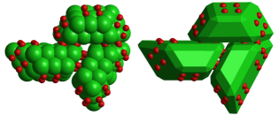
Figure 16: Fully-bonded trimer showing the spheres that define each particle, the bonding sites (in red) and the effective particle shape.

The soft spheres on different particles interact via the usual short-range repulsion (1). In order to define the bonding forces needed for assembly, several interaction sites are located on the lateral faces of each particle, shown in Figure 16, and attractive forces can act between corresponding sites on specific face pairs of different particles (consistent with the particle arrangement in the final shell structure); the use of multiple interaction sites on each face ensures that maximum attraction is achieved only when particles are properly aligned. The interaction has the form of an inverse power law over most of its range, but at small distances $<r_{h}$, it changes smoothly into a stretched harmonic spring,

$$u_{a}(r)=\left\{\begin{array}[]{ll}e(1/r_{a}^{2}+r^{2}/r_{h}^{4}-2/r_{h}^{2})&\quad r<r_{h}\\ e(1/r_{a}^{2}-1/r^{2})&\quad r_{h}\leq r<r_{a}\end{array}\right.$$ (8)

where $e$ is the overall attraction strength that will be regarded as an adjustable parameter. The range of the attractive force, $r_{a}=3$, is similar to the particle size (whose edge lengths vary between 2.1 and 3.6), and the crossover distance is $r_{h}=0.3$; this relatively narrow harmonic well helps minimize structural fluctuations. While the attraction between individual site pairs has no directional dependence, the involvement of several pairs contributes to correct particle positioning and orientation, further enhancing the rigidity of multiply-bonded structures. A side-effect of the minimal structural fluctuations is that the final stages of shell assembly are prolonged, because incoming particles must be correctly aligned to fit into available openings that leave minimal room for maneuvering.

In order to carry out quantitative analysis of the cluster structure, those particle pairs in which all four sets of matching attraction sites lie within a prescribed (and arbitrary) range $r_{b}$ are considered bonded. There is nothing special about bond formation since it is merely a bookkeeping device, and the process is entirely reversible, a factor that turns out to be central to successful assembly. A value of $r_{b}=0.5$ ($>r_{h}$) leads to results consistent with direct observation, namely that structural fluctuations are responsible for only minimal spurious bond breakage and no false bond designation. Each set of bonded particles forms a cluster. Since the particle design and parameterization ensures that bonded pairs have very limited relative motion, the only possible cluster in which every particle has a full complement of five bonded neighbors is a closed shell of size 60; mutant clusters do not develop for the range of $e$ considered here.

The simulations also include an explicit atomistic solvent, represented by the same soft spheres (with repulsive interactions only) used in constructing the particles. A thermostat is incorporated in the solvent dynamics to regulate temperature [3]; this is especially important in view of the energy released as particles approach to within bonding range. The explicit solvent entails significant computational cost, but offers increased realism over the implicit (stochastic) alternative. While both are capable of serving as heat baths to absorb the bond formation energy, as well as curtailing the ballistic nature of the particle motion to ensure conditions closer to thermal equilibrium, only the explicit approach allows particles that have assembled into structures to offer mutual shielding against disruptive solvent effects, aids cluster breakup without subassemblies needing to collide directly, and incorporates the dynamical correlations of the fluid medium. The choice of solvent representation is also capable of affecting the outcome of self-assembly simulations [101]. The size ratio of the particles relative to the solvent atoms is much smaller than in reality, in order to enhance particle mobility and compress the time scales over which assembly occurs; the corresponding mass ratio (here 15) is also reduced. Additional details appear in [99].

Maximizing the yield of complete shells is an important goal in formulating the model; the fact that the region size is limited makes this a more important issue than it would be in vivo where other considerations (of a more biological nature) are involved. Since allowing bond breakage might be expected to reduce efficiency, the approach used both in the original simulations [96] and as one of the alternatives in [97] (see also [102]) is to make bond formation irreversible (accomplished by altering the form of the pair attraction once inside a suitably defined bonding range, together with a complicated procedure aimed at avoiding bonds incompatible with the final structure). In practice, it turns out that not only is reversible bonding much simpler from a computational point of view (with incompatible bonds left to break on their own) but, paradoxically, reversibility is a key contributor to efficient assembly [98, 99]. Indeed, reversibility constitutes a major difference between assembly at microscopic and macroscopic scales, and is a consequence of the thermal ‘noise’ that competes with the forces driving growth, an effect practically invisible at the macroscopic level (where Brownian motion offers a mere hint of its existence).

The large system described here has a total size of $N=2.16\times 10^{5}$, almost twice that of [99] (where $1.25\times 10^{5}$), to determine the effect of size on the outcome. It includes $N_{p}=4752$ particles, enough for 79 complete shells of size 60, and a solvent with $N_{a}=N-N_{p}$ atoms. The particle fraction is the same as before, namely $p=N_{p}/N=0.022$. The overall number density is 0.1; this determines the volume of the cubic simulation region, and is a compromise that ensures the solvent can fulfill its role while not excessively impeding particle motion. The interaction strength parameter $e$ is set to 0.09, the value producing the highest shell yield in the earlier work.

Figure 17 shows the system at an early stage of the run, after $5\times 10^{4}$ timesteps, where only monomers are apparent. The final state, after $3.2\times 10^{8}$ timesteps, appears in Figure 18; the remaining monomers and solvent are omitted from the image so that the relevant particles can be seen. Here, the 57 complete shells that have formed can be seen (after allowing for the periodic boundaries), a 72% yield fraction, and just three incomplete clusters. This picture of perfectly formed, self-assembled structures should be contrasted with the previous image of an almost homogeneous early state (which, in fact, includes eight probably-transient dimers).

The growth history of the shells, expressed in terms of the time- and size-dependent distribution of the cluster mass fraction, is shown in Figure 19. The most notable feature of the graph is the final state, which contains essentially only complete shells and a significant residual monomer population; with the exception of just three almost complete shells, intermediate-size clusters are entirely absent. During the period over which most of the growth occurs the size distribution is relatively broad and ill-defined, a consequence of the considerable variation in the growth histories of individual clusters. Faint traces of shells that are late developers are also apparent.

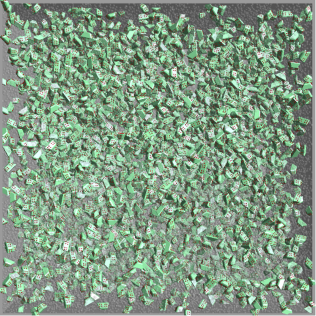
Figure 17: Early state of the large self-assembly simulation; the space-filling solvent is shown semitransparently.

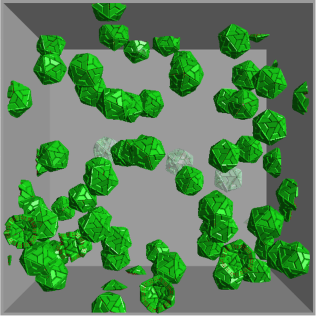
Figure 18: The final self-assembled state; monomers and solvent are omitted and incomplete clusters are shown in a lighter color; because of periodic boundaries some complete shells appear as fragments on opposite sides of the region.

Figure 19: The cluster mass fraction distribution for the large system as a function of time; late in the run the system consists almost entirely of complete shells and monomers.

The lesson remains unchanged: given suitable parameters, it is possible to achieve a final state consisting almost entirely of a high population of complete shells and monomers. The successful self-assembly pathway, as revealed by a more detailed analysis of cluster development [99], comprises a cascade of reversible stages, with smaller clusters showing a distinct preference for maximally bonded (i.e., low-energy) states, eventually leading to a high yield of complete shells. This outcome is attributable to the fact that reversibility maintains a low growth initiation probability, while at the same time allowing breakage of any incorrect bonds that might attempt to form; alternative, less desirable scenarios, such as minimal aggregation, multiple small clusters, and clusters with unlimited growth, are all avoided. Reversibility dominates the development of the smallest clusters, with dimers typically have just a 1% probability of growing into trimers (at $e=0.09$), and trimers 50% to tetramers; over the broad size range 4–50 the probability of a unit size increment is only $\approx 60\%$.

Once a closed shell has formed breakup is practically impossible. This is a result of each particle being restrained by all five of its bonds, and the absence of structural fluctuations capable of breaking individual bonds and so initiate structural failure. This form of hysteresis was demonstrated directly in [98], by showing that if $e$ is reduced during the run to a level at which assembly would not have occurred, all unfinished (and therefore less strongly bound) assemblies disappear, leaving only the complete shells.

Multiple runs of identical systems starting from different initial states reveal substantial variations in the number of complete shells. This is due to the two rate-limiting growth stages, namely the low probability of successfully initiating shell assembly by growing well beyond the dimer and trimer clusters, and the prolonged delay for the final couple of assembly steps to complete due to the difficulty of inserting the last monomers into the small holes in the shell. Results from three runs are compared in Figure 20. Two of the runs are for the smaller system with different initial states, one of which is taken from [99]. The differences between the complete-shell curves typify the variability of the results; since the final state consists principally of complete shells and monomers, the variations in the monomer mass fraction mirror those of the complete shells. The third run is the large system, where the fact that the fractional shell yield lies between the yields of the two smaller systems shows that doubling the size leaves the behavior unchanged. In view of the low survival probability of small clusters, successful initiation of shell growth can be regarded as a rare event, with consequences extending over the entire growth process and eventually affecting the yield of complete shells. In this respect, the outcome resembles the previous case studies, where effects amounting to little more than noise are capable of altering the principal features of the final result.

Figure 20: Time-dependent mass fractions for the large (solid curves, unfilled symbols) and small (long dashes) systems, together with the earlier small system [99] (short dashes, only monomers and complete shells shown); results are grouped into size ranges, the monomer curves are without symbols, and there is no contribution from the size range 2–5.

The final cluster distribution depends on $e$, with moderate to high yields appearing only over a relatively narrow range; thus it is conceivable that the high-yield phenomenon could easily have gone unnoticed. Results showing the strong variation of the final distributions with $e$ for a 2.2% particle fraction, i.e., $p=0.022$, were described in [99]. Similar behavior occurs for other $p$; as an example, the final cluster distributions of the smaller system ($N=1.25\times 10^{5}$) at $p=0.033$ are tabulated in Table 1 for various $e$. Allowing for the inherent fluctuations, these results show the same kind of sensitive $e$-dependence as for smaller $p$, ranging from no growth, through moderate and high yields of complete shells, to a mixture of sizes but no complete shells as $e$ is increased (note that raising $e$ is roughly equivalent to reducing temperature).

When the particle fraction is lowered to $p=0.015$, the shell yield is greatly reduced for runs of length similar to those considered here, although the possibility of continued slow growth cannot be excluded since ample supplies of monomers remain. Given the increased elapsed time between monomer encounters, and the short dimer lifetime, such a result is to be expected, with the implication that a significant effort will be required for computing the complete $p$ – $e$ phase diagram. In view of the protracted final stage of the assembly process, any comparison of the yields for different $p$ and $e$ values, as required for the phase diagram evaluation, might consider counting the nearly-complete shells together with the complete shells, as well as taking into account whether the residual monomer population is sufficient to fill the remaining holes given sufficient time. A similar grouping of complete and nearly-complete shells is relevant for comparison with experiment, since physical properties dependent on cluster size might not be affected by a few small gaps in the shells.

Table 1: Final cluster mass fractions for different interaction strengths $e$, grouped by cluster size (particle fraction $p=0.033$).

• $e$	Timesteps	Cluster mass fraction
  	($\times 10^{6}$)	Size: 1	2–50	51–59	60
  0.080	158	0.991	0.009	0	0
  0.085	141	0.514	0.006	0.029	0.451
  0.088	171	0.278	0.010	0.014	0.698
  0.090	307	0.043	0.036	0.383	0.538
  0.095	85	0.018	0.479	0.503	0

6 Outlook

A variety of systems exhibiting different forms of emergent behavior have been studied using MD simulation. The phenomena associated with these systems involve hydrodynamic instability, granular segregation and supramolecular self-assembly. The most prominent feature in each of the simulations is the emergence of a specific kind of ordered behavior associated with, respectively, the flow patterns, spatial organization and structure formation.

Although these problems have little in common, apart from the MD methodology, since they deal with different systems and modes of behavior on scales ranging from the molecular to the macroscopic, they share an ability to produce effects that are both interesting and surprising. Given the computationally-limited scope of MD simulation, the ability to achieve such a rich set of outcomes is far from obvious. There are numerous reasons for such skepticism, among them the possibility of capturing hydrodynamic behavior within the relatively small spatial and temporal scales covered by atomistic fluid simulation, the capability of simple frictional models to replicate the complex behavior of granular mixtures (for one of the cases considered, and predicting hitherto unknown behavior in the other), and the ability of complex self-assembly processes to reach completion sufficiently rapidly. The fact that each of the studies managed to generate meaningful results is encouraging, as are the future prospects, given (still) ever-increasing computational power and the availability of multiscale methods (not covered here) to expand the simulational horizon.

An issue common to the problems considered here is reproducibility. The kind of self-averaging that allows equating the results of a single MD simulation to the ensemble average of statistical mechanics does not apply to the most prominent results of the present case studies, namely the organization of the induced flows, the spatial arrangement of the segregated regions, and the yield of complete shells, nor to the intermediate stages of the processes leading to these outcomes. Ensuring the reliability of any conclusions based on these simulations requires repeating each of the runs sufficiently many times to establish the ‘average’ behavior and the range of possible alternatives; this applies to each interesting parameter combination, adding to the computational cost. It goes without saying that the same lack of detailed reproducibility is intrinsic to the actual physical systems that the simulations aim to emulate.

Finally, it is conceivable that there are some useful developments in mathematics [103] which might not have been forthcoming had ‘modern’ computers and their algorithms been available in an earlier era, especially since the need to solve real physical problems was a motivating factor. The absence of mathematical tools capable of addressing the inherent complexity of emergent phenomena, despite ample motivation, guarantees the role of computational exploration for the foreseeable future.

References

References

- [1] Alder B J and Wainwright T E 1957 J. Chem. Phys. 27 1208
- [2] Rahman A 1964 Phys. Rev. 136A 405
- [3] Rapaport D C 2004 The Art of Molecular Dynamics Simulation 2nd ed (Cambridge: Cambridge University Press)
- [4] Rapaport D C 2011 Computer Phys. Comm. 182 926
- [5] van Dyke M 1982 An Album of Fluid Motion (Stanford, CA: Parabolic)
- [6] Alder B J and Wainwright T E 1970 Phys. Rev. A 1 18
- [7] Rapaport D C and Clementi E 1986 Phys. Rev. Lett. 57 695
- [8] Rapaport D C 1987 Phys. Rev. A 36 3288
- [9] Mareschal M and Kestemont E 1987 J. Stat. Phys. 48 1187
- [10] Rapaport D C 1988 Phys. Rev. Lett. 60 2480
- [11] Puhl A, Mansour M M and Mareschal M 1989 Phys. Rev. A 40 1999
- [12] Rapaport D C 1992 Phys. Rev. A 46 1971
- [13] Rapaport D C 1992 Phys. Rev. A (Rapid Communication) 46 R6150
- [14] Chandrasekhar S 1961 Hydrodynamic and Hydromagnetic Stability (Oxford: Oxford University Press)
- [15] Kadau K, Germann T C, Hadjiconstantinou N G, Lomdahl P S, Dimonte G, Holian B L and Alder B J 2004 PNAS 101 5851
- [16] Moseler M and Landman U 2000 Science 289 1165
- [17] Taylor G I 1923 Philos. Trans. R. Soc. London A 223 289
- [18] Drazin P G and Reid W H 1981 Hydrodynamic Stability (Cambridge: Cambridge University Press)
- [19] Cole J A 1976 J. Fluid Mech. 75 1
- [20] Andereck C D, Liu S S and Swinney H L 1986 J. Fluid Mech. 164 155
- [21] Di Prima R C and Swinney H L 1981 Hydrodynamic Instabilities and the Transition to Turbulence ed Swinney H L and Gollub J P (Berlin: Springer) p 139
- [22] Marcus P S 1984 J. Fluid Mech. 146 65
- [23] Lücke M, Mihelcic M and Wingerath K 1985 Phys. Rev. A 31 396
- [24] Donnelly R J, Schwarz K W and Roberts P H 1965 Proc. R. Soc. Lond. A 283 531
- [25] Snyder H A and Lambert R B 1966 J. Fluid Mech. 26 545
- [26] Gollub J P and Freilich M H 1976 Phys. Fluids 19 618
- [27] Berland T, Jossang T and Feder J 1986 Physica Scripta 34 427
- [28] Heinrichs R M, Cannell D S, Ahlers G and Jefferson M 1988 Phys. Fluids 31 250
- [29] Wereley S T and Lueptow R M 1994 Experiments in Fluids 18 1
- [30] Hirshfeld D and Rapaport D C 1998 Phys. Rev. Lett. 80 5337
- [31] Hirshfeld D and Rapaport D C 2000 Phys. Rev. E (Rapid Communication) 61 R21
- [32] Benjamin T B and Mullin T 1982 J. Fluid Mech. 121 219
- [33] Davey A 1962 J. Fluid Mech. 14 336
- [34] Normand C, Pomeau Y and Velarde M G 1977 Rev. Mod. Phys. 49 581
- [35] Bergé P and Dubois M 1984 Contemp. Phys. 25 535
- [36] Koschmieder E L 1993 Bénard Cells and Taylor Vortices (Cambridge: Cambridge University Press)
- [37] Bodenschatz E, Pesch W and Ahlers G 2000 Annu. Rev. Fluid Mech. 32 709
- [38] Goldhirsch I, Pelz R B and Orszag S A 1989 J. Fluid. Mech. 199 1
- [39] Gelfgat A Y 1999 J. Comput. Phys. 156 300
- [40] Watanabe T and Kaburaki H 1997 Phys. Rev. E 56 1218
- [41] Rapaport D C 2006 Phys. Rev. E (Rapid Communication) 73 025301
- [42] Assenheimer M and Steinberg V 1996 Phys. Rev. Lett. 76 756
- [43] Bajaj K M S, Cannell D S and Ahlers G 1997 Phys. Rev. E 55 R4869
- [44] Roy A and Steinberg V 2002 Phys. Rev. Lett. 88 244503
- [45] Barker G C 1994 Granular Matter: An Interdisciplinary Approach ed Mehta A (Heidelberg: Springer) p 35
- [46] Herrmann H J 1995 3rd Granada Lectures in Computational Physics ed Garrido P L and Marro J (Heidelberg: Springer) p 67
- [47] Jaeger H M, Nagel S R and Behringer R P 1996 Rev. Mod. Phys. 68 1259
- [48] Kadanoff L P 1999 Rev. Mod. Phys. 71 435
- [49] Cundall P A and Strack O D L 1979 Géotechnique 29 47
- [50] Walton O R 1983 Mechanics of Granular Materials ed Jenkins J T and Satake M (Amsterdam: Elsevier) p 327
- [51] Haff P K and Werner B T 1986 Powder Tech. 48 239
- [52] Seiden G and Thomas P J 2011 Rev. Mod. Phys. 83 1323
- [53] Zik O, Levine D, Lipson S G, Shtrikman S and Stavans J 1994 Phys. Rev. Lett. 73 644
- [54] Hill K M, Caprihan A and Kakalios J 1997 Phys. Rev. E 56 4386
- [55] Nakagawa M, Altobelli S A, Caprihan A and Fukushima E 1997 Chem. Eng. Sci. 52 4423
- [56] Frette V and Stavans J 1997 Phys. Rev. E 56 6981
- [57] Choo K, Baker M W, Molteno T C A and Morris S W 1998 Phys. Rev. E 58 6115
- [58] Alexander A, Muzzio F J and Shinbrot T 2004 Gran. Matter 5 171
- [59] Arndt T, Siegmann-Hegerfeld T, Fiedor S J, Ottino J M and Lueptow R M 2005 Phys. Rev. E 71 011306
- [60] Finger T, Voigt A, Stadler J, Niessen H G, Naji L and Stannarius R 2006 Phys. Rev. E 74 031312
- [61] Aranson I S and Tsimring L S 2006 Rev. Mod. Phys. 78 641
- [62] Rapaport D C 2007 Phys. Rev. E 75 031301
- [63] Rapaport D C 2007 Phys. Rev. E 76 041302
- [64] Farkas Z, Tegzes P, Vukics A and Vicsek T 1999 Phys. Rev. E 60 7022
- [65] Levanon M and Rapaport D C 2001 Phys. Rev. E 64 011304
- [66] Rosato A, Strandburg K J, Prinz F and Swendsen R H 1987 Phys. Rev. Lett. 58 1038
- [67] Gallas J A C, Herrmann H J, Pöschel T and Sokolowski S 1996 J. Stat. Phys. 82 443
- [68] Rapaport D C 2001 Phys. Rev. E 64 061304
- [69] Crick F H C and Watson J D 1956 Nature (Lond.) 177 473
- [70] Caspar D L D and Klug A 1962 Cold Spring Harbor Symp. Quant. Biol. 27 1
- [71] Baker T S, Olson N H and Fuller S D 1999 Microbiol. Mol. Biol. Rev. 63 862
- [72] Prevelige P E, Thomas D and King J 1993 Biophys. J. 64 824
- [73] Casini G L, Graham D, Heine D, Garcea R L and Wu D T 2004 Virology 325 320
- [74] Zlotnick A and Mukhopadhyay S 2011 Trends in Microbiol. 19 14
- [75] Caspar D L D 1980 Biophys. J. 32 103
- [76] Hagan M F and Chandler D 2006 Biophys. J. 91 42
- [77] Freddolino P L, Arkhipov A S, Larson S B, McPherson A and Schulten K 2006 Structure 14 437
- [78] Nguyen H D, Reddy V S and Brooks III C L 2007 Nano Letters 7 338
- [79] Chen T, Zhang Z and Glotzer S C 2007 Proc. Natl. Acad. Sci. USA 104 717
- [80] Wilber A W, Doye J P K, Louis A A, Noya E G, Miller M A and Wong P 2007 J. Chem. Phys. 127 085106
- [81] Johnston I G, Louis A A and Doye J P K 2010 J. Phys.: Condens. Matter 22 104101
- [82] Hagan M F 2014 Adv. Chem. Phys. 155 1
- [83] Breen T L, Tien J, Oliver S R J, Hadzic T and Whitesides G M 1999 Science 284 948
- [84] Lidmar J, Mirny L and Nelson D R 2003 Phys. Rev. E 68 051910
- [85] Zandi R, Reguera D, Bruinsma R F, Gelbart W M and Rudnick J 2004 Proc. Natl. Acad. Sci. USA 101 15556
- [86] Twarock R 2004 J. Theor. Biol. 226 477
- [87] Hemberg M, Yaliraki S N and Barahona M 2006 Biophys. J. 90 3029
- [88] Hicks S D and Henley C L 2006 Phys. Rev. E 74 031912
- [89] Zandi R, van der Schoot P, Reguera D, Kegel W and Reiss H 2006 Biophys. J. 90 1939
- [90] Moisant P, Neeman H and Zlotnick A 2010 Biophys. J. 99 1350
- [91] Morozov A Y, Bruinsma R F and Rudnick J 2009 J. Chem. Phys. 131 155101
- [92] Hagan M F and Elrad O 2010 Biophys. J. 98 1065
- [93] Zlotnick A, Johnson J M, Wingfield P W, Stahl S J and Endres D 1999 Biochemistry 38 14644
- [94] van der Schoot P and Zandi R 2007 Phys. Biol. 4 296
- [95] Zlotnick A 2007 J. Mol. Biol. 366 14
- [96] Rapaport D C, Johnson J E and Skolnick J 1999 Comp. Phys. Comm. 121 231
- [97] Rapaport D C 2004 Phys. Rev. E 70 051905
- [98] Rapaport D C 2008 Phys. Rev. Lett. 101 186101
- [99] Rapaport D C 2012 Phys. Rev. E 86 051917
- [100] Endres D and Zlotnick A 2002 Biophys. J. 83 1217
- [101] Spaeth J R, Kevrekidis I G and Panagiotopoulos A Z 2011 J. Chem. Phys. 134 164902
- [102] Rapaport D C 2010 Phys. Biol. 7 045001
- [103] Wigner E P 1960 Comm. Pure App. Math. 13 1