Constructing Cartesian Splines

Abstract.

We introduce here Cartesian splines or, for short, C-splines. C-splines are piecewise polynomials which are defined on adjacent Cartesian coordinate systems and are $C^{r}$ continuous throughout. The $C^{r}$ continuity is enforced by constraining the coefficients of the polynomial to lie in the null-space of some smoothness matrix $H$. The matrix-product of the null-space of the smoothness matrix $H$ and the original polynomial base results in a new base, the so-called C-spline base, which automatically enforces $C^{r}$ continuity throughout. In this article we give a derivation of this C-spline base as well as an algorithm to construct C-spline models.

1. Introduction

We introduce here Cartesian splines or, for short, C-splines. C-splines are piecewise polynomials which are defined on adjacent Cartesian coordinate systems and are $C^{r}$ continuous throughout. The $C^{r}$ continuity is enforced by constraining the coefficients of the polynomial to lie in the null-space of some smoothness matrix $H$. The matrix-product of the null-space of the smoothness matrix $H$ and the original polynomial base results in a new base, the so-called C-spline base, which automatically enforces $C^{r}$ continuity throughout. The idea of using the null-space of some smoothness matrix $H$ has been taken from the B-spline literature, where piecewise polynomials are defined on adjacent triangular Barycentric coordinate systems, [1]. It turns out that C-spline bases have a particular simple form. This makes it possible to give an explicit formulation of general C-spline bases. In this article we will give a general outline how to enforce continuity constraints by way of the smoothness matrix $H$. We then show how these constraints lead us to the C-spline base. Then we will give the explicit algorithm for constructing a bivariate C-spline base and show how to use this base to construct a C-spline model.

2. Piecewise Polynomials

We start with the bivariate Cartesian $x$,$y$-coordinate system. We partition this initial coordinate system with origin $O=\left(0,0\right)$ in two adjacent coordinate systems, each with its own origin, $O=\left(0,0\right)$ and $\tilde{O}=\left(0,0\right)$. The geometry in terms of $x$ and $y$ may be depicted as:

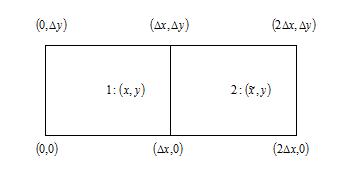
Figure 1. Geometry of the domain of two piecewise polynomials in terms of $x$ and $y$

where $\Delta x$ and $\Delta y$ are some constants. Likewise, the geometry in terms of $\tilde{x}$ and $y$ may be depicted as:

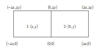
Figure 2. Geometry of the domain of two piecewise polynomials in terms of $\tilde{x}$ and $y$

where $\Delta x$ and $\Delta y$ are the same constants as used in Figure 1.

Now, we may define on both coordinate systems a polynomial of order $d$:

$$P_{d}\left(x,y\right)=\sum_{0\leq p+q\leq d}c_{pq}x^{p}y^{q}$$ (2.1)

We start with the most simple case, that is, we set $d=1$. The polynomial equations for both coordinate systems then become:

$$z_{1}\left(x,y\right)=c_{11}+c_{12}x+c_{13}y,\quad\quad 0\leq x\leq\Delta x,\quad 0\leq y\leq\Delta y$$

$$z_{2}\left(\tilde{x},y\right)=c_{21}+c_{22}\tilde{x}+c_{23}y,\quad\quad 0\leq\tilde{x}\leq\Delta x,\quad 0\leq y\leq\Delta y$$ (2.2)

If we look at Figure 2, we see that

$$\tilde{x}=x-\Delta x$$ (2.3)

Combining (2) and (2.3) we get:

$$z_{1}\left(x,y\right) =c_{11}+c_{12}x+c_{13}y,\quad \;\;\;0\leq x\leq\Delta x,\quad\;\;0\leq y\leq\Delta y$$

$$z_{2}\left(x,y\right) =c_{21}+c_{22}\left(x-\Delta x\right)+c_{23}y,\quad \Delta x\leq x\leq 2\Delta x,\quad 0\leq y\leq\Delta y$$ (2.4)

Let

$$\mathbf{z}=\begin{pmatrix}z_{1}\left(x,y\right)&z_{2}\left(x,y\right)\end{pmatrix}^{T}$$

be the outcome vector. Then (2) may be rewritten as the matrix-vector product of the polynomial base

$$B=\begin{pmatrix}1&x&y&0&0&0\\ 0&0&0&1&x-\Delta x&y\end{pmatrix}$$ (2.5)

and the coefficient vector

$$\mathbf{c}=\begin{pmatrix}c_{11}&c_{12}&c_{13}&c_{21}&c_{22}&c_{23}\end{pmatrix}^{T}$$ (2.6)

that is,

$$\mathbf{z}=B\mathbf{c}$$

Note that the $\left(x,y\right)$-values that fall in the first quadrant of Figure 1 are assigned to the first row of the polynomial base $B$, while $\left(x,y\right)$-values in the second quadrant are assigned to the second row.

3. Enforcing Zeroth Order Continuity

In order for the two polynomials (2) to connect at the boundary, that is, in order to have $C^{0}$ continuity, we must have that

$$z_{1}\left(\Delta x,y\right)=z_{2}\left(\Delta x,y\right)$$ (3.1)

for any $y$. Substituting (2) in (3.1), we find

$$c_{11}+c_{12}\Delta x+c_{13}y=c_{21}+c_{23}y$$

or, equivalently,

$$c_{11}+c_{12}\Delta x+c_{13}y-c_{21}-c_{23}y=0$$ (3.2)

We have that (3.2) is a constraint on the $\mathbf{c}$ coefficients. The coefficients $\mathbf{c}$ must all lie in the null-space of the smoothness “matrix” $H$, where

$$H=\begin{pmatrix}1&\Delta x&y&-1&0&-1\end{pmatrix}$$ (3.3)

The null-space of $H$ is

$$H_{0}=\begin{pmatrix}y&0&1&-y&-\Delta x\\ 0&0&0&0&1\\ 0&0&0&1&0\\ 0&0&1&0&0\\ 0&1&0&0&0\\ 1&0&0&0&0\end{pmatrix}$$ (3.4)

and it may be checked that

$$HH_{0}=\mathbf{0}$$

where $\mathbf{0}$ is the $1\times 5$ zero vector. It follows that the matrix product of $H$ with any linear combination of the columns in $H_{0}$ must give a zero value, that is,

$$HH_{0}\mathbf{c}_{0}=0$$

where $\mathbf{c}_{0}$ is an arbitrary $5\times 1$ vector. Stated differently, any linear combination of the columns of $H_{0}$ gives us an $6\times 1$ vector that satisfies the constraint (3.1) or, equivalently, constraint (3.2).

Now, if we take the matrix product of our original polynomial base, $B$, and the null-space of our smoothness matrix, $H_{0}$, we get the null-base $B_{0}$:

$$B_{0} =BH_{0}$$

$$=\begin{pmatrix}y&0&1&0&x-\Delta x\\ y&x-\Delta x&1&0&0\end{pmatrix}$$ (3.5)

If we drop the zero column in (3) and rearrange the columns somewhat, we get the C-spline base, $B_{C}$:

$$B_{C}=\begin{pmatrix}1&y&x-\Delta x&0\\ 1&y&0&x-\Delta x\end{pmatrix}$$ (3.6)

Let

$$\mathbf{b}=\begin{pmatrix}b_{1}&b_{2}&b_{3}&b_{4}\end{pmatrix}^{T}$$

be an arbitrary coefficient vector. Then

$$\mathbf{z}=B_{C}\mathbf{b}$$

corresponds with the polynomial equations

$$z_{1}\left(x,y\right)=b_{1}+b_{2}y+b_{3}\left(x-\Delta x\right),\quad\quad \;\;\;0\leq x\leq\Delta x,\quad\;\;0\leq y\leq\Delta y$$

$$z_{2}\left(x,y\right)=b_{1}+b_{2}y+b_{4}\left(x-\Delta x\right),\quad\quad \Delta x\leq x\leq 2\Delta x,\quad 0\leq y\leq\Delta y$$ (3.7)

Now, if we substitute $x=\Delta x$ in (3) we have that for any choice of $\mathbf{b}$ constraint (3.1) is satisfied:

$$z_{1}\left(\Delta x,y\right)=z_{2}\left(\Delta x,y\right)=b_{1}+b_{2}y$$ (3.8)

It follows that $B_{C}$, (3.6), is the base that enforces zeroth order continuity.

We summarize, $C^{0}$ continuity between two piecewise polynomials results in a smoothness matrix $H$, (3.3). The coefficients $\mathbf{c}$, (2.6), defined on the original polynomial base $B$, (2.5), are constrained to lie within the null-space of this smoothness matrix. Stated differently, the coefficients $\mathbf{c}$ are constrained to be a linear combination of the columns of $H_{0}$, (3.4), which span the null space of $H$. By directly multiplying the null-space matrix $H_{0}$ with the the original polynomial base $B$ we get the null-base $B_{0}$, (3), which contains redundant columns consisting of zero vectors. Dropping these zero vectors we obtain the C-spline base $B_{C}$, (3.6), which has the $C^{0}$ constraint (3.1) build into its structure, as may be checked, (3.8).

4. Enforcing First Order Continuity

In order for the partial derivatives of the two polynomials (2) to connect at the boundary, that is, in order to have $C^{1}$ continuity, we must have that the partial derivatives $\partial z_{1}/\partial x$ and $\partial z_{2}/\partial x$ are $C^{0}$ at their boundaries, that is

$$\left.\frac{\partial z_{1}\left(x,y\right)}{\partial x}\right|_{x=\Delta x}=\left.\frac{\partial z_{2}\left(x,y\right)}{\partial x}\right|_{x=\Delta x}$$ (4.1)

Substituting (2) in  (4.1), we find

$$c_{12}=c_{22}$$

or, equivalently,

$$c_{12}-c_{22}=0$$ (4.2)

Adding constraint (4.2) to (3.3), the new smoothness matrix $H$ and the corresponding null space $H_{0}$ become, respectively,

$$H=\begin{pmatrix}&1&\Delta x&y&-1&0&-1\\ &0&1&0&0&-1&0\end{pmatrix}$$

and

$$H_{0}=\begin{pmatrix}y&-\Delta x&1&-y\\ 0&1&0&0\\ 0&0&0&1\\ 0&0&1&0\\ 0&1&0&0\\ 1&0&0&0\end{pmatrix}$$ (4.3)

Multiplying (4.3) with the original polynomial base (2.5) we get

$$B_{0} =BH_{0}$$

$$=\begin{pmatrix}y&x-\Delta x&1&0\\ y&x-\Delta x&1&0\end{pmatrix}$$

Dropping the redundant zero column and rearranging the columns somewhat, we get the C-spline base:

$$B_{C}=\begin{pmatrix}1&y&x-\Delta x\\ 1&y&x-\Delta x\end{pmatrix}$$ (4.4)

which, since $\Delta x$ is a constant, is equivalent to the base

$$B_{C}=\begin{pmatrix}1&y&x\\ 1&y&x\end{pmatrix}$$ (4.5)

From C-spline-base (4.5) it can be seen that the first order piecewise polynomials which have first order partial derivatives everywhere collapse to a global polynomial of order $d=1$ and $C^{1}$, which is just the base of a linear regression model having an intercept and predictors $x$ and $y$.

The here given framework for deriving C-spline bases may be generalized to $d$th order piecewise polynomials with $r$th order continuity, $0\leq r\leq d$, on arbitrary geometries. If one does this then it is found that the C-spline base, $B_{C}$, has a relatively simple structure. This simple structure allows us to directly construct $B_{C}$ without first having to compute the null matrix $H_{0}$ and then taking its matrix product with the original base $B$. This makes C-spline modeling, as given in the next section, computationally efficient. It will be seen that the computational burden of constructing a C-spline is equivalent to that of performing an ordinary regression analysis.

5. An Algorithm to Construct C-Splines

We give here the algorithm for the construction of C-splines for bivariate geometries, partitioned into $I\times J$ adjacent Cartesian domains on which $d$th order piecewise polynomials with $r$th order continuity everywhere are defined.

5.1. The Geometry

First we define a partitioning of the Cartesian $\left(x,y\right)$ plane. Then we number the resulting partitionings. In the region of interest the $x$ values take on values from $a_{x}$ to $b_{x}$ and the $y$ values take on values from $a_{y}$ to $b_{y}$. If we partition the $x$-axis in $I$ adjacent axes with equal lengths $\Delta x$ and the $y$-axis in $J$ adjacent axes with equal lengths $\Delta y$. Then this results in $K=IJ$ partitionings.

Now, we may number each partitioning in the following manner. For $i=1$ we number the partitionings of the $y$-axis from $k=1,\ldots,J$ , for $i=2$ we number the partitionings of the $y$-axis from $k=J+1,\ldots,2J$ , etc We then have that the $\left(i,j\right)$th partitioning is numbered as

$$k=\left(i-1\right)J+j,\qquad\qquad\qquad 1\leq i\leq I,\qquad 1\leq j\leq J$$ (5.1)

where $k=1,\ldots,K$ and $K=IJ$.

In the next paragraph we will construct our C-spline base. The geometry, as given in (5.1), is non-trivial in that the Cartesian coordinate system having coordinates $\left(i,j\right)$ corresponds with the $k$th row of this C-spline base.

5.2. Constructing the C-Spline Base

First we construct the building blocks of our base. Let

$$u_{i}=\begin{cases}\left(x-a_{x}\right)-i\Delta x,\quad\quad&i=1,\ldots,I-1\\ \left(x-a_{x}\right)-\left(i-1\right)\Delta x,\quad\quad&i=I\end{cases}$$ (5.2)

Then the $x$-columns of the building blocks are:

$$u_{ki}=\begin{cases}u_{i},\quad\quad&k=1,\ldots,iJ,\quad\quad\begin{cases}i=1,\ldots,I\end{cases}\\ 0,\quad\quad&else\end{cases}$$ (5.3)

where $k=1,\ldots,K$ and $K=IJ$. Likewise, let

$$v_{j}=\begin{cases}\left(y-a_{y}\right)-j\Delta y,\quad\quad&j=1,\ldots,J-1\\ \left(y-a_{y}\right)-\left(j-1\right)\Delta y,\quad\quad&j=J\end{cases}$$ (5.4)

Then the $y$-columns of the building blocks are:

$$v_{kj}=\begin{cases}v_{j},\quad\quad&k=1,\ldots,j+\left(i-1\right)\times J,\quad\quad\begin{cases}j=1,\ldots,J\\ i=1,\ldots,I\end{cases}\\ 0,\quad\quad&else\end{cases}$$ (5.5)

where $k=1,\ldots,K$ and $K=IJ$.

Using the building blocks (5.3) and (5.5), we may now construct the C-spline base $B_{C}$. Our polynomial is of order $d$, that is, let $p$ and $q$ be the powers of $x$ and $y$, respectively, then $0\leq p+q\leq d$. Let

$$U_{p}=\begin{cases}u_{kI}^{p},\quad\quad&p\leq r\\ \left\{u_{k1}^{p},\ldots,u_{kI}^{p}\right\},\quad\quad&p>r\end{cases}$$ (5.6)

$$V_{q}=\begin{cases}v_{kJ}^{q},\quad\quad&q\leq r\\ \left\{v_{k1}^{q},\ldots,v_{kJ}^{q}\right\},\quad\quad&q>r\end{cases}$$ (5.7)

Then we take the outer product of $U_{p}$ and $V_{q}$ to get $B_{p,q}$, the C-spline equivalent of the polynomial term $x^{p}y^{q}$:

$$B_{p,q}=U_{p}\otimes V_{q}=\begin{cases}u_{kI}^{p}v_{kJ}^{q},\quad\quad&p\leq r,q\leq r\\ \\ \left\{u_{kI}^{p}v_{k1}^{q},u_{kI}^{p}v_{k2}^{q},\ldots,u_{kI}^{p}v_{kJ}^{q}\right\},\quad\quad&p\leq r,q>r\\ \\ \left\{u_{k1}^{p}v_{kJ}^{q},u_{k2}^{p}v_{kJ}^{q},\ldots,u_{kI}^{p}v_{kJ}^{q}\right\},\quad\quad&p>r,q\leq r\\ \\ \left\{u_{k1}^{p}v_{k1}^{q},u_{k1}^{p}v_{k2}^{q},\ldots,u_{kI}^{p}v_{kJ}^{q}\right\},\quad\quad&p>r,q>r\\ \end{cases}$$ (5.8)

Just as the collection of terms $\left\{x^{p}y^{q}\right\}_{0\leq p+q\leq d}$ span the polynomial $P_{d}$, (2.1), So the collection of column vectors

$$B_{C}\left(x,y\right)=\left\{B_{p,q}\right\}_{0\leq p+q\leq d}$$ (5.9)

span the piecewise polynomials that make up the C-spline.

Note that for the geometry $I=2$, $J=1$, polynomial order $d=1$ and continuity order $r=0$, the C-spline base (5.9) will differ from (3.6) by one column permutation. Both bases may be considered equivalent in that they both enforce constraint (3.1).

5.3. Assigning Data Points to the C-Spline Base

We have $N$ observed data points in the Cartesian $\left(x,y\right)$-plane that are related to some observed point on the $z$-axis through the unknown function $f$, that is

$$f\left(x_{n},y_{n}\right)=z_{n},\qquad\qquad n=1,\ldots,N.$$ (5.10)

By using base (5.9), we approximate the unknown function $f$ with a collection of piecewise polynomials of degree $d$ that are $C^{r}$ continuous everywhere. To do this we first have to assign each data point $\left(x_{n},y_{n}\right)$ to its corresponding partitioning.

The $x$- and $y$-axes of each partitioning have,see paragraph 5.1, lengths of

$$\Delta x=\frac{b_{x}-a_{x}}{I},\quad\quad\Delta y=\frac{b_{y}-a_{y}}{J}$$

We then have that for the data point $\left(x_{n},y_{n}\right)$ which lies in the partitioning having coordinates $\left(i,j\right)$:

$$a_{x}+\left(i-1\right)\Delta x\leq x_{n} \leq a_{x}+i\Delta x,$$

$$a_{y}+\left(j-1\right)\Delta y\leq y_{n} \leq a_{y}+j\Delta y$$

or, equivalently,

$$\left(i-1\right)\leq\frac{x_{n}-a_{x}}{\Delta x}\leq i,\quad\quad\left(j-1\right)\leq\frac{y_{n}-a_{y}}{\Delta y}\leq j$$

It follows that the coordinates of the partitioning in which the data point $\left(x_{n},y_{n}\right)$ lies may be found as

$$i=ceil\left(\frac{x_{n}-a_{x}}{\Delta x}\right),\quad j=ceil\left(\frac{y_{n}-a_{y}}{\Delta y}\right)$$ (5.11)

where $ceil\left(x\right)$ is the function that gives the smallest integer that is greater than or equal to $x$. Substituting these coordinates in (5.1), we may assign the data point $\left(x_{n},y_{n}\right)$ to its corresponding piecewise polynomial, or, equivalently, to its corresponding row $k$ in the base (5.9).

Example:
Say, we use the C-spline base as given in (3.6)

$$B_{C}\left(x,y\right)=\begin{pmatrix}1&y&x-\Delta x&0\\ 1&y&0&x-\Delta x\end{pmatrix}$$

where the first and second row of $B_{C}$ correspond, respectively, with the first and second partitioning of Figure 1. Now, say we have a small dataset of $N=5$ observations $\left(x_{n},y_{n}\right)$ having values of

$$\left(x_{1},y_{1}\right) =\left(1.1\Delta x,0.3\Delta y\right)$$

$$\left(x_{2},y_{2}\right) =\left(1.2\Delta x,0.7\Delta y\right)$$

$$\left(x_{3},y_{3}\right) =\left(0.1\Delta x,0.3\Delta y\right)$$

$$\left(x_{4},y_{4}\right) =\left(0.5\Delta x,0.1\Delta y\right)$$

$$\left(x_{5},y_{5}\right) =\left(1.7\Delta x,0.8\Delta y\right)$$

where $\Delta x$ and $\Delta y$ are some constants. Then, using (5.1) and (5.11), the points $\left(x_{3},y_{3}\right)$ and $\left(x_{4},y_{4}\right)$ are assigned to the first partitioning, or, equivalently, to the first row of $B_{C}$. Likewise, $\left(x_{1},y_{1}\right)$, $\left(x_{2},y_{2}\right)$ and $\left(x_{5},y_{5}\right)$ are assigned to the second partitioning, or, equivalently, to the second row of $B_{C}$:

$$\tilde{B}_{C}=\begin{pmatrix}B_{C}^{\left(2\right)}\left(x_{1},y_{1}\right)\\ B_{C}^{\left(2\right)}\left(x_{2},y_{2}\right)\\ B_{C}^{\left(1\right)}\left(x_{3},y_{3}\right)\\ B_{C}^{\left(1\right)}\left(x_{4},y_{4}\right)\\ B_{C}^{\left(2\right)}\left(x_{5},y_{5}\right)\end{pmatrix}=\begin{pmatrix}1&0.3\Delta y&0&0.1\Delta x\\ 1&0.7\Delta y&0&0.2\Delta x\\ 1&0.3\Delta y&-0.9\Delta x&0\\ 1&0.1\Delta y&-0.5\Delta x&0\\ 1&0.8\Delta y&0&0.7\Delta x\end{pmatrix}$$ (5.12)

Note that we use a tilde to signify a base $B_{C}$ to which data points have been assigned.

5.4. Constructing a C-Spline

Let $m$ be the number of columns of the C-spline base $B_{C}$, (5.9). Then, after we have assigned all $N$ data points to the base $B_{C}$, we get the $N\times m$ matrix $\tilde{B}_{C}$, see (5.12). The unknown b coefficients, see (3), of the C-spline may be found as the least-squares solution of

$$\textbf{b}=\left(\tilde{B}_{C}^{T}\tilde{B}_{C}\right)^{-1}\tilde{B}_{C}^{T}\textbf{z}$$ (5.13)

where $\textbf{z}=\begin{pmatrix}z_{1}&\cdots&z_{N}\end{pmatrix}$ is the vector with output values, (5.10).

Now, say we wish to get the C-spline estimate $\hat{z}_{N+1}$ of the data point $\left(x_{N+1},y_{N+1}\right)$. Then, using (5.1) and (5.11), we first determine the row $k$ of the base $B_{C}$, (5.9), that corresponds with this data point and then plug in its value. This results in the $1\times m$ row-vector

$$\tilde{B}_{C}^{\left(k\right)}=B_{C}^{\left(k\right)}\left(x_{N+1},y_{N+1}\right)$$ (5.14)

The estimate $\hat{z}_{N+1}$ is then found by simply taking the inner product of (5.14) and (5.13):

$$\hat{\textbf{z}}=\tilde{B}_{C}^{\left(k\right)}\cdot\textbf{b}$$

We see that constructing a C-spline is equivalent to performing a regression analysis.

6. Discussion

We have introduced here Cartesian splines, or C-splines, for short. C-splines are piecewise polynomials which are defined on adjacent Cartesian coordinate systems and are $C^{r}$ continuous throughout. We have given here an algorithm that allows one to construct C-spline bases without first having to find the null-space of the corresponding smoothness matrix $H$.

This makes the construction of a given C-spline base computationally trivial since no null-space of $H$ has to be evaluated. This means that for C-splines the computational burden lies solely, just as in any ordinary regression analysis, in the evaluation of the inverse of $\tilde{B}_{C}^{T}\tilde{B}_{C}$, where $\tilde{B}_{C}$ is the matrix with the independent variables.

Note that the algorithm, equations (5.1) through (5.9), may be generalized relatively easy to construct C-splines for multivariate domains.

Acknowledgments: This research was partly funded by the Delft Cluster project (no. CT04.33.11), which is kindly acknowledged by the authors.

References

- [1] Awanou G. Energy Methods in 3D Spline Approximations of Navier-Stokes Equations. Ph.D. thesis, University of Georgia, Athens, Georgia, 2003.