The NLO contributions to the scalar pion form factors and the ${\cal O}(\alpha_{s}^{2})$ annihilation corrections to the $B\to\pi\pi$ decays

Abstract

In this paper, by employing the $k_{T}$ factorization theorem, we made the first calculation for the space-like scalar pion form factor $Q^{2}F(Q^{2})$ at the leading order (LO) and the next-to-leading order (NLO) level, and then found the time-like scalar pion form factor $F^{\prime(1)}_{\rm a,I}$ by analytic continuation from the space-like one. From the analytical evaluations and the numerical results, we found the following points: (a) the NLO correction to the space-like scalar pion form factor has an opposite sign with the LO one but is very small in magnitude, can produce at most $10\%$ decrease to LO result in the considered $Q^{2}$ region; (b) the NLO time-like scalar pion form factor $F^{\prime(1)}_{\rm a,I}$ describes the ${\cal O}(\alpha_{s}^{2})$ contribution to the factorizable annihilation diagrams of the considered $B\to\pi\pi$ decays, i.e. the NLO annihilation correction; (c) the NLO part of the form factor $F^{\prime(1)}_{\rm a,I}$ is very small in size, and is almost independent with the variation of cutoff scale $\mu_{0}$, but this form factor has a large strong phase around $-55^{\circ}$ and may play an important role in producing large CP violation for $B\to\pi\pi$ decays; and (d) for $B^{0}\to\pi^{+}\pi^{-}$ and $\pi^{0}\pi^{0}$ decays, the newly known NLO annihilation correction can produce only a very small enhancement to their branching ratios, less than $3\%$ in magnitude, and therefore we could not interpret the well-known $\pi\pi$-puzzle by the inclusion of this NLO correction to the factorizable annihilation diagrams.

I Introduction

As an important application of the $k_{\rm T}$ factorization theorem plb242-97 ; npb325-62 ; npb360-3 ; npb366-135 ; npb381-129 ; zpc50-139 ; prd52-5358 , the perturbative QCD (pQCD) factorization approach prd53-2480 ; prd63-074009 ; prd65-014007 ; epjc23-275 ; prd66-094010 has been widely used to deal with various $B/B_{s}$ meson decays for example in Refs.prd72-114005 ; prd86-114025 ; prd87-094003 ; prd90-014029 ; csb59-125 . One advantage of the pQCD factorization approach is that the annihilation diagrams in the heavy-to-light decays are calculableprd67-034001 . In pQCD approach, the annihilation diagrams can provide a large strong phase which is essential to generate the large CP violation for some $B/B_{s}$ meson decay channels.

In recent years, the $k_{\rm T}$ factorization theorem is greatly improved after intensive studies by many authors. By using the universal gauge invariant wave functions with the inclusion of high order contributions prd64-014019 ; epjc40-395 ; jhep0601-067 , the next-to-leading order (NLO) corrections to the form factors for some transition processes have been calculated prd76-034008 ; prd83-054029 ; prd85-074004 ; prd89-054015 ; prd89-094004 during the past decade.

1. The pion form factors in $\pi\gamma^{\star}\to\gamma$ transition were calculated in Ref. prd76-034008 . The authors found that the NLO correction is only $\sim 5\%$ of the leading order (LO) one when the factorization scale set to be equal with the momentum transfer.

2. The pion electromagnetic form factors in $\pi\gamma^{\star}\to\pi$ transition were calculated in Refs.prd83-054029 ; prd89-054015 . The total NLO contribution can provide a roughly $\sim 20\%$ enhancement to the LO contribution in the considered ranges of the momentum transfer $Q^{2}$;

3. The $B\to\pi$ transition form factors involved in the semi-leptonic decay $B\to\pi l\overline{\nu}$ were calculated in Refs.prd85-074004 ; prd89-094004 . The NLO contribution from twist-2 part of the wave function cam provide $\sim 30\%$ correction to the LO order one prd85-074004 , but it is largely canceled by the NLO Twist-3 contribution prd89-094004 , and finally result in a net $\sim 8\%$ enhancement to the LO result.

4. In Ref. plb693-102 , the combined analysis of the space-like and time-like electromagnetic pion form factors has been done in the light-cone pQCD, with the inclusion of the non-perturbative ”soft” QCD and the twist-3 corrections.

5. The NLO corrections to the time-like pion transition form factor and the electromagnetic pion form factors have been calculated in Ref.plb718-1351 , where the NLO twist-2 correction to the magnitude (phase) are found to be smaller than $30\%(30^{\circ})$ for the time-like pion transition form factors, and lower than $25\%(10^{\circ})$ for the time-like electromagnetic form factors at the large invariant mass squared $Q^{2}>30$ GeV².

One should note that the vertices for all above mentioned transitions and decay processes involve the vector currents only. The NLO corrections to the form factors with a scalar vertex, however, have not been evaluated up to now.

As is well known, the B meson physics is an wonderful place to test the standard model (SM) and to search for the signal of the new physics (NP) beyond the SM. For the two body charmless hadronic $B/B_{s}\to h_{1}h_{2}$ decays (here $h_{i}$ refers to the light pseudo-scalar or vector mesons ), such as $B^{\pm}\to\pi^{\pm}\pi^{0}$ and $B^{0}\to\pi^{+}\pi^{-}$ decays, the major contribution come from the factorizable emission diagrams, in which the space-like form factors with the vector current are involved. But for the color-suppressed $B^{0}\to\pi^{0}\pi^{0}$ decay, along with a large cancelation between the emission diagrams, the contribution from the annihilation diagrams play an important role: the corresponding amplitude is proportional to the complex time-like scalar pion form factor.

In the framework of the pQCD factorization approach, the calculations for the main part of the NLO contributions from various sources have been done during the past decade for example in Refs. prd72-114005 ; prd85-074004 ; prd89-094004 ; plb718-1351 , the still missing NLO part in the pQCD approach includes the ${\cal O}(\alpha^{2}_{s})$ contributions from the hard spectator diagrams and annihilation diagrams. In this paper, we will make the first calculation for the scalar pion form factors up to NLO in the $k_{\rm T}$ factorization theorem, which has a direct relation with the evaluation of NLO contributions from those annihilation diagrams of $B/B_{s}\to h_{1}h_{2}$ decays.

For this purpose, we firstly give a brief review for the LO space-like and time-like scalar pion form factors. Secondly, we will calculate the NLO corrections to the space-like scalar pion form factor, in which the momentum transfer squared is $q^{2}=-Q^{2}<0$. Thirdly, by analytic continuation from $q^{2}=-Q^{2}<0$ to $q^{2}=Q^{2}>0$, we will obtain the NLO correction to the time-like scalar pion form factors from the one for the space-like scalar pion form factor. We finally evaluate the relevant annihilation diagrams, and to check the effects on the branching ratios of $B\to\pi\pi$ induced by the inclusion of the newly found NLO correction to the time-like scalar pion form factors.

By using the universal NLO pion meson wave functions (twist-2 and twist-3 part) as defined in Refs. prd67-034001 ; prd64-014019 ; epjc40-395 ; jhep0601-067 , we will make the convolutions of the LO hard kernel and the NLO wave functions, evaluate the quark level diagrams for the NLO corrections to the LO scalar transition process $\pi\to\pi$, and finally obtain an infrared (IR) finite NLO hard kernel by making the difference of these two parts. All the IR singularities, such as the soft divergences generated from exchanging a massless gluon between two on-shell external quark lines and/or the collinear divergences generated from emitting a massless gluon from a light parallelled external quark line, are regulated by the off-shell transverse momentum $k_{\rm iT}$.

We will verify that all the IR divergences obtained from the NLO calculations can be absorbed into the NLO wave functions completely as described in Refs. prd83-054029 ; prd89-054015 . The analytic continuations of the NLO correction to the space-like scalar pion form factor to the one on the time-like scalar pion form factor is also nontrivial. When we make the appropriate choice for the renormalization scale $\mu$ and the factorization scale $\mu_{f}$, say setting them as the internal hard scale $t$ as postulated in Refs. prd83-054029 ; prd89-054015 ; plb718-1351 , we find that the NLO corrections on both the space-like and the time-like scalar form factors are indeed under control naturally.

This paper is organized as follows. In Sec. II, we give a brief review about the LO space-like and time-like scalar pion form factors and show the analytic continuation relation between them. In Sec. III, we calculate the NLO correction to the space-like scalar pion form factor and present the numerical results. In this section, the $O(\alpha^{2}_{s})$ QCD quark diagrams, as well as the convolutions between LO hard kernel and NLO wave functions, will be calculated step by step, and then obtain the $k_{\rm T}$-dependent NLO hard kernel by making the difference between the two parts. Sec. IV contains the analytic continuation of the scalar pion form factor from the space-like domain $q^{2}=-Q^{2}<0$ to the time-like domain $q^{2}=Q^{2}>0$. We will calculate the branching ratios for $B\to\pi\pi$ decays, and to check if the “$\pi\pi$”-puzzle could be understood by the inclusion of the newly known NLO contribution to the time-like scalar pion form factor. Section V finally contains the conclusions.

II Leading order analysis

We first give a brief review about the LO space-like and time-like scalar pion form factors in the framework of the $k_{\rm T}$ factorization.

Figure 1: The LO quark diagrams for the space-like scalar pion form factors for transition $\pi\to\pi$, with the symbol $\bullet$ representing the insertion of the scalar interaction vertex.

For the space-like form factor at leading order, the relevant Feynman diagrams are illustrated in Fig. 1, where the symbol $\bullet$ representing the insertion of the scalar interaction vertex. The momentum transfer squared is

$$q^{2}=(p_{2}-p_{3})^{2}=-2p_{2}\cdot p_{3}\equiv-Q^{2},\quad{\rm with}\quad Q^{2}>0,$$ (1)

where $p_{2}$ and $p_{3}$ are the momentum carried by the initial and final state meson

$$p_{2}=(p^{+}_{2},0,{\textbf{0}_{\rm T}}),\quad p_{3}=(0,p^{-}_{3},{\textbf{0}_{\rm T}}).$$ (2)

While the momentum $k_{2}$ and $k_{3}$ carried by the anti-quark in the initial and final state mesons can be written as

$$k_{2}=(x_{2}p^{+}_{2},0,{\textbf{k}_{\rm 1T}}),\quad k_{3}=(0,x_{3}p^{-}_{3},{\textbf{k}_{\rm 2T}}),$$ (3)

where $x_{2}$ and $x_{3}$ are the momentum fractions of the anti-quark.

Figure 2: The LO factorizable annihilation diagrams for $B\to\pi\pi$ decays, in which the time-like scalar pion form factors are involved. The symbol $\bullet$ here represent the effective weak decay vertex.

For the time-like case as shown in Fig. 2, the momentum of the initial state B meson are set as

$$p_{1}=(p^{+}_{1},p^{-}_{1},{\textbf{0}_{\rm T}}),$$ (4)

with the light anti-quark inside the B meson carrying the momentum $k_{1}=(x_{1}p^{+}_{1},0,{\textbf{k}_{\rm 1T}})$. The final state mesons $M_{2}$ and $M_{3}$, produced from the B meson decay, have the momentum

$$p_{2}=(p^{+}_{2},0,{\textbf{0}_{\rm T}}),\quad p_{3}=(0,p^{-}_{3},{\textbf{0}_{\rm T}}),$$ (5)

and the momentum carried by their partons are defined as $k_{2}=(x_{2}p^{+}_{2},0,{\textbf{k}_{\rm 2T}})$ and $k_{3}=(0,x_{3}p^{-}_{3},{\textbf{k}_{\rm 3T}})$ as shown in Fig. 2 explicitly. But the momentum transfer squared in this process is $q^{2}=(p_{2}+p_{3})^{2}=M^{2}_{B}>0$ with $M_{B}$ being the B meson mass.

Besides the two Feynman diagrams as given in Fig. 1, in fact, there exist other two Feynman diagrams with the vertex located in the lower anti-parton lines, which also contribute to the space-like scalar pion form factor at the leading order. But we here just want to evaluate the NLO corrections to the time-like scalar pion form factors, which should contribute through the annihilation diagrams of the $B\to M_{2}M_{3}$ decays, as illustrated in Fig. 2. For this purpose, only the two Feynman diagrams as shown in Fig. 1 should be calculated firstly and then we can find the time-like scalar pion form factors from the space-like ones by making the analytical continuations. So, we here only consider the two diagrams as given in Fig. 1.

II.1 Leading order space-like scalar pion form factor

Because the vertex in Fig. 1 are scalar in nature, the scalar pion form factors at LO level can be written directly from the hard kernels of the sub-diagrams in Fig. 1. The following hierarchy is postulated in the small-x region in our analytic calculation, as in Res. prd83-054029 ; prd89-054015 :

$$Q^{2}\gg x_{1}Q^{2}\sim x_{2}Q^{2}\gg x_{1}x_{2}Q^{2}\gg{\textbf{k}_{\rm 1T}}^{2}\sim{\textbf{k}_{\rm 2T}}^{2}.$$ (6)

We use the Fierz identity in Eq. (7) and the $SU(3)_{c}$ group identity in Eq. (8) to factorize the fermion flow and the color flow. The identity matrix $I$ in the Fierz identity is a $4$-dimension matrix and $(i,j,l,k)$ are the Lorentz index, while the identity matrix $I$ in the $SU(3)_{C}$ group is a $3$-dimension matrix and $(i,j,l,k)$ are color index.

$$I_{ij}I_{lk} = \frac{1}{4}I_{ik}I_{lj}+\frac{1}{4}(\gamma_{5})_{ik}(\gamma_{5})_{lj}+\frac{1}{4}(\gamma^{\alpha})_{ik}(\gamma^{\alpha})_{lj}$$ (7)

$$+\frac{1}{4}(\gamma_{5}\gamma^{\alpha})_{ik}(\gamma_{\alpha}\gamma_{5})_{lj}+\frac{1}{8}(\sigma^{\alpha\beta}\gamma_{5})_{ik}(\sigma_{\alpha\beta}\gamma_{5})_{lj},$$

$$I_{ij}I_{lk} = \frac{1}{N_{c}}I_{lj}I_{ik}+2(T^{c})_{lj}(T^{c})_{ik}.$$ (8)

Because the weak vertex in Fig. 1(a) is proportional to identity $I$ in the Lorentz space, then we can obtain the hard kernel $H^{(0)}_{a}$ by sandwiching Fig. 1(a) with the following two sets of structures of pion wave functions:

$$\left(\frac{p/_{2}\gamma_{5}}{4N_{c}},\quad\frac{\gamma_{5}}{4N_{c}}~{}or~{}\frac{\gamma_{5}(n/_{-}n/_{+})}{4N_{c}}\right);~{}~{}~{}\left(\frac{\gamma_{5}}{4N_{c}}~{}or~{}\frac{\gamma_{5}(n/_{-}n/_{+})}{4N_{c}},\quad\frac{\gamma_{5}p/_{3}}{4N_{c}}\right),$$ (9)

where $n_{+}=(1,0,{\textbf{0}_{\rm T}})$ and $n_{-}=(0,1,{\textbf{0}_{\rm T}})$ denote the unit vector along with the positive and negative $z$-axis direction. Of course, one can write down $H^{(0)}_{a}$ directly by using the initial and the final pion meson wave functionsprd65-014007 ; zpc48-239 ; jhep9901-010 ; jhep0605-004 ; prd71-014015 ; csb59-3801 as given explicitly in Eqs. (10,11) with the chiral mass of pion $m_{0\pi}=1.74$ GeV:

$$\Phi_{\pi}(p_{2},x_{2}) = \frac{1}{\sqrt{6}}\Bigl{\{}p/_{2}\gamma_{5}\phi_{\pi}^{A}(x_{2})+m_{0\pi}\gamma_{5}\left[\phi^{P}_{\pi}(x_{2})-(n/_{-}n/_{+}-1)\phi^{T}_{\pi}(x_{2})\right]\Bigr{\}},$$ (10)

$$\Phi_{\pi}(p_{3},x_{3}) = \frac{1}{\sqrt{6}}\Bigl{\{}\gamma_{5}p/_{3}\phi_{\pi}^{A}(x_{3})+\gamma_{5}m_{0\pi}\left[\phi^{P}_{\pi}(x_{3})-(n/_{-}n/_{+}-1)\phi^{T}_{\pi}(x_{3})\right]\Bigr{\}}.$$ (11)

Then the LO contributions to the hard kernel from Fig. 1(a) can be written as

$$H^{(0)}_{a}(x_{2},x_{3},Q^{2}) = \frac{8\pi\alpha_{s}C_{F}m_{0\pi}Q^{2}}{(p_{3}-k_{2})^{2}(k_{2}-k_{3})^{2}}$$ (12)

$$\cdot\Bigl{\{}2\phi^{A}_{\pi}(x_{2})\phi^{P}_{\pi}(x_{3})+x_{2}\left[\phi^{P}_{\pi}(x_{2})-\phi^{T}_{\pi}(x_{2})\right]\phi^{A}_{\pi}(x_{3})\Bigr{\}}.$$

where $\alpha_{s}$ is the strong coupling constant, $C_{F}=4/3$ is the color factor. It is not difficult to find the end-point behavior of the LO hard kernel for Fig. 1(a):

$$H^{(0)}_{a}(x_{2},x_{3},Q^{2})|_{\rm end-point} \to (16\pi\alpha_{s}C_{F}m_{0\pi}Q^{2})\cdot\Bigl{\{}\frac{(1-x_{2})}{x_{2}x_{3}}+(1-x_{3})\Bigr{\}},$$ (13)

where the first and second term describes the end-point behavior of the corresponding term in Eq. (12). It is easy to verify that the second term in Eq. (13) is strongly suppressed by a factor of $x_{2}x_{3}(1-x_{3})/(1-x_{2})$ relative to the first term. The first term proportioned to $\phi^{A}(x_{3})\phi^{P}(x_{2})$ in Eq. (12), consequently, will provide the dominate contribution when compared with the second term in Eq. (12). The numerical results as illustrated by the curves in Fig. 3 confirmed this point directly.

By using the LO hard kernel $H^{(0)}_{a}$ in Eq. (12), one can find the corresponding space-like scalar pion form factor at the LO level in the form of

$$Q^{2}F(Q^{2})|_{\rm LO} = 8\pi m_{0\pi}C_{F}Q^{4}\int{dx_{2}dx_{3}}\int{b_{2}db_{2}b_{3}db_{3}}$$ (14)

$$\cdot\Bigl{\{}2\phi^{A}_{\pi}(x_{2})\phi^{P}_{\pi}(x_{3})S_{t}(x_{3})+x_{2}\left[\phi^{P}_{\pi}(x_{2})-\phi^{T}_{\pi}(x_{2})\right]\phi^{A}_{\pi}(x_{3})\Bigr{\}}$$

$$\cdot\alpha_{s}(t)\cdot e^{-2S_{\pi}(t)}\cdot h(x_{2},x_{3},b_{2},b_{3}),$$

where the Sudakov factor $S_{\pi}(t)$ and the threshold resummation function $S_{t}(x)$ are the same ones as being used in Refs. prd65-014007 ; prd89-054015 . In numerical calculation we choose $c=0.4$ in the function $S_{t}(x)$. The hard function $h(x_{2},x_{3},b_{2},b_{3})$ in Eq. (14) can be written as the following form

$$h(x_{2},x_{3},b_{2},b_{3}) = K_{0}\left(\sqrt{x_{2}x_{3}}Qb_{2}\right)$$ (15)

$$\cdot\Bigl{[}\theta(b_{2}-b_{3})I_{0}\left(\sqrt{x_{3}}Qb_{3}\right)K_{0}\left(\sqrt{x_{3}}Qb_{2}\right)+(b_{2}\leftrightarrow b_{3})\Bigr{]},$$

where the function $K_{0}$ and $I_{0}$ are the modified Bessel function. Following Refs. prd83-054029 ; prd89-054015 , we here also choose $\mu=\mu_{f}=t$ in the numerical calculations:

$$\mu=\mu_{f}=t=\max\left(\sqrt{x_{2}}Q,\sqrt{x_{3}}Q,1/b_{2},1/b_{3}\right).$$ (16)

In the calculations, we can consider the sub-diagram Fig. 1(a) only, since the contributions from Fig. 1(b) can be obtained by simple kinematic replacements of $x_{2}\leftrightarrow x_{3}$ for the results from the Fig. 1(a) as we have argued in Ref. prd89-054015 . The direct analytical evaluations for Fig. 1(b) can verify this exchange symmetry. After making the analytic calculations we found the expressions for the LO hard kernel $H^{(0)}_{b}(x_{1},x_{2},Q^{2})$ and its end-point behavior:

$$H^{(0)}_{b}(x_{2},x_{3},Q^{2}) = \frac{8\pi\alpha_{s}C_{F}m_{0\pi}Q^{2}}{(p_{2}-k_{3})^{2}(k_{3}-k_{2})^{2}}$$ (17)

$$\cdot\Bigl{\{}2\phi^{A}_{\pi}(x_{3})\phi^{P}_{\pi}(x_{2})+x_{3}\left[\phi^{P}_{\pi}(x_{3})-\phi^{T}_{\pi}(x_{3})\right]\phi^{A}_{\pi}(x_{2})\Bigr{\}},\ \$$

$$H^{(0)}_{b}(x_{2},x_{3},Q^{2})|_{\rm end-point} \rightarrow (16\pi\alpha_{s}C_{F}m_{0\pi}Q^{2})\cdot\Bigl{\{}\frac{(1-x_{3})}{x_{2}x_{3}}+(1-x_{2})\Bigr{\}}.$$ (18)

In Fig. 3, we show the $Q^{2}$-dependence of the LO space-like scalar pion form factor $Q^{2}F(Q^{2})$ for Fig. 1(a), in order to support our previous theoretical arguments for the dominance of the contribution from the first term of the hard kernel $H^{(0)}_{a}(x_{2},x_{3},Q^{2})$ as defined in Eq. (12). In Fig. 3, the contributions from the two different terms as given in Eq. (12) are plotted explicitly: the upper dot-dashed curve with the label ”LO₁” shows the contribution from the first term proportional to $2\phi^{P}_{\pi}(x_{2})\phi^{A}_{\pi}(x_{3})$ in the LO hard kernel $H^{(0)}_{a}$, while the lower doted curve with the label ”LO₂” shows the contribution from the second term in $H^{(0)}_{a}$, and finally the solid line denotes the total LO contribution. One can see from the curves in Fig. 3 that the contribution to the LO space-like scalar pion form factor $Q^{2}F(Q^{2})$ from the first term of $H^{(0)}_{a}$ is indeed dominant absolutely, larger than $90\%$ of the total LO result in the whole considered range of $Q^{2}$.

Figure 3: The LO pQCD prediction for the space-like scalar pion form factor $Q^{2}F(Q^{2})$ from Fig. 1(a). For more details see the text.

In the numerical calculations, we integrate for the partons’ momentum fractions ($x_{2},x_{3}$) over the range of $x_{i}=[0,1]$, and find that the main contribution comes from the small $x_{2},x_{3}\sim 0.1$ region prd66-094010 , being consistent with the hierarchy postulated in Eq. (6) for our analytic calculation. After the numerical integration, we obtained the LO theoretical predictions as shown in Fig. 3 by using the the ordinary full pion distribution amplitudes(DA’s) as given in Refs. prd71-014015 ; jhep0605-004 :

$$\phi_{\pi}^{A}(x) = \frac{3f_{\pi}}{\sqrt{6}}x(1-x)\left[1+a_{2}^{\pi}C_{2}^{\frac{3}{2}}(u)+a_{4}^{\pi}C_{4}^{\frac{3}{2}}(u)\right],$$

$$\phi_{\pi}^{P}(x) = \frac{f_{\pi}}{2\sqrt{6}}\left[1+\left(30\eta_{3}-\frac{5}{2}\rho_{\pi}^{2}\right)C_{2}^{\frac{1}{2}}(u)-3\left(\eta_{3}\omega_{3}+\frac{9}{20}\rho_{\pi}^{2}\left(1+6a_{2}^{\pi}\right)\right)C_{4}^{\frac{1}{2}}(u)\right],$$

$$\phi_{\pi}^{T}(x) = \frac{f_{\pi}}{2\sqrt{6}}(1-2x)\left[1+6\left(5\eta_{3}-\frac{1}{2}\eta_{3}\omega_{3}-\frac{7}{20}\rho_{\pi}^{2}-\frac{3}{5}\rho_{\pi}^{2}a_{2}^{\pi}\right)\left(1-10x+10x^{2}\right)\right],$$

where the pion decay constant $f_{\pi}=0.13$ GeV, the Gegenbauer moments $a_{i}^{\pi}$, the parameters $\eta_{3},\omega_{3}$ and $\rho_{\pi}$ are adapted from Refs. jhep0605-004 ; prd71-014015 :

$$a_{2}^{\pi} = 0.25\pm 0.015,\quad a_{4}^{\pi}=-0.015,\quad\rho_{\pi}=m_{\pi}/m^{0}_{\pi},\quad\eta_{3}=0.015,\quad\omega_{3}=-3.0.$$ (20)

The relevant Gegenbauer polynomials $C_{2,4}^{1/2}(2x-1)$ and $C_{2,4}^{3/2}(2x-1)$ can be found easily in Refs. jhep0605-004 ; prd71-014015 .

From the expressions of the LO hard kernels $H^{(0)}_{a},H^{(0)}_{b}$ as given in Eqs. (12,17) and the LO pQCD predictions for $Q^{2}F(Q^{2})$ as illustrated in Fig. 3, one can see the following points:

1. The LO hard kernel $H^{(0)}$ only receive the contributions from the two cross productions of the DA’s with different twists for the initial and final pion wave function, because of the nature of the scalar current in the vertex of Fig. 1. Take $H^{(0)}_{a}$ as an example, the contributions do come from the two terms proportional to $\phi^{A}(x_{2})\phi^{P}(x_{3})$ and $[\phi^{P}(x_{2})-\phi^{T}(x_{2})]\phi^{A}(x_{3})$ respectively, as listed in Eq. (12).

2. From Fig. 3 one can see easily that the first term in the LO hard kernel $H_{a}^{(0)}$ in Eq. (12) provides the absolutely dominant contribution (larger than $90\%$) to the form factor $Q^{2}F(Q^{2})$ in the whole region of $1<Q^{2}<30$ GeV², while the contribution from the second term of $H_{a}^{(0)}$ in Eq. (12) is very small and can be neglected safely. This fact does support our previous argument from the analysis for the end-point behavior of the two terms in Eqs. (13,18).

3. Since the LO contribution from the second term of $H^{(0)}_{a}$ in Eq. (12) is already very small, it is reasonable for us to consider the NLO contribution to the space-like scalar pion form factor from the dominant first term in $H^{(0)}_{a}$ only in next section, which would simplify our calculations significantly.

II.2 Leading order time-like scalar pion form factor

The weak decay vertices in the factorizable annihilation diagrams for B decays, as shown in Fig. 2, would generate three kinds of contributions: $(V-A)\otimes(V-A)$, $(V-A)\otimes(V+A)$ and $(S-P)\otimes(S+P)$ current contribution. We here abbreviate these contributions as LL, LR and SP current respectively. The SP current comes from the Fierz transformation of the LR current if the light anti-quarks in B meson and one of the final light mesons are identical. In this paper, we will just consider the SP current proportioned to the time-like scalar pion form factors, because the LO hard kernels with the LL and LR currents are canceled each other completely in Fig. 2(a) and Fig. 2(b) when the two final states have the same wave functions, as described in detail in Ref. prd63-074009 .

Using the definition of the annihilation matrix element $<0|(\bar{q}b)_{S-P}|B(p_{1})>=if_{B}M_{B}$, the LO hard kernel for Fig. 2(a) and 2(b) can be written in the following form:

$$H^{\prime(0)}_{a}(x_{2},k_{\rm 2T};x_{3},k_{\rm 3T};M^{2}_{B}) = \frac{-8\pi\alpha_{s}C_{F}m^{0}_{\pi}M^{2}_{B}(-2if_{B}M_{B})}{[(p_{1}-k_{3})^{2}+i\epsilon]](k_{3}-p_{3}-k_{2})^{2}+i\epsilon]}$$ (21)

$$\cdot\Bigl{\{}(1-x_{3})\phi^{A}_{\pi}(x_{2})\left[\phi^{P}_{\pi}(x_{3})+\phi^{T}_{\pi}(x_{3})\right]+2\phi^{P}_{\pi}(x_{2})\phi^{A}_{\pi}(x_{3})\Bigr{\}},$$

$$H^{\prime(0)}_{b}(x_{2},k_{\rm 2T};x_{3},k_{\rm 3T};M^{2}_{B}) = \frac{-8\pi\alpha_{s}C_{F}m^{0}_{\pi}M^{2}_{B}(-2if_{B}M_{B})}{[(k_{3}-p_{3}-k_{2})^{2}+i\epsilon][(p_{3}+k_{2})^{2}+i\epsilon]}$$ (22)

$$\cdot\Bigl{\{}x_{2}\left[\phi^{P}_{\pi}(x_{2})-\phi^{T}_{\pi}(x_{2})\right]\phi^{A}_{\pi}(x_{3})+2\phi^{A}_{\pi}(x_{2})\phi^{P}_{\pi}(x_{3})\Bigr{\}}.$$

It’s easy to confirm that the LO hard amplitude $H^{\prime(0)}_{b}$ can be obtained from $H^{\prime(0)}_{a}$ by simple kinetic replacements $x_{3}\leftrightarrow(1-x_{2})$, we therefore could deal with the Fig. 2(a) in our calculation and get the one for Fig. 2(b) by proper kinetic replacements $x_{3}\leftrightarrow(1-x_{2})$.

Furthermore, the contribution to $H^{\prime(0)}_{a}$ mainly comes from the small $(1-x_{3})\sim 0.1$ region due to the threshold suppression effectsprd66-094010 , while the contribution proportional to term $\phi^{A}_{\pi}(x_{2})\left[\phi^{P}_{\pi}(x_{3})+\phi^{T}_{\pi}(x_{3}\right]$ in $H^{\prime(0)}_{a}$ is also suppressed by the factor $x_{2}(1-x_{2})(1-x_{3})/x_{3}$. It is therefore reasonable for us to consider the dominant $H^{\prime(0)}_{a,32}$ proportioned to term $\phi^{P}_{\pi}(x_{2})\phi^{A}_{\pi}(x_{3})$ only when we calculate the hard amplitude $H^{\prime(0)}_{a}$:

$$H^{\prime(0)}_{a,32}(x_{2},k_{\rm 2T};x_{3},k_{\rm 3T};M^{2}_{B})\equiv\frac{-16\pi\alpha_{s}C_{F}m^{0}_{\pi}M^{2}_{B}(-2if_{B}M_{B})}{[(p_{1}-k_{3})^{2}+i\epsilon][(k_{3}-p_{3}-k_{2})^{2}+i\epsilon]}\phi^{P}_{\pi}(x_{2})\phi^{A}_{\pi}(x_{3}).\ \$$ (23)

For the Fourier transformation of Eq. (21) from the transverse-momentum space $({\textbf{k}_{\rm 2T}},{\textbf{k}_{\rm 3T}})$ to the impact-parameter space $(b_{2},b_{3})$, we have two different choices: One is the double-b convolution, another is the single-b convolution.

If one write the two factors in the denominator of the hard kernel in Eqs. (21,23) in the form of

$$(p_{1}-k_{3})^{2}+i\epsilon = M^{2}_{B}(1-x_{3})-{\textbf{k}_{\rm 3T}}^{2}+i\epsilon;$$

$$(k_{3}-p_{3}-k_{2})^{2}+i\epsilon = M^{2}_{B}x_{2}(1-x_{3})-({\textbf{k}_{\rm 3T}}-{\textbf{k}_{\rm 2T}})^{2}+i\epsilon,$$ (24)

one could obtain, after making the integration of the hard kernel in Eq. (21) over the whole momentum space, the complex time-like amplitudes which may provide a strong phase to generate the large CP violation observed for example in $B\to\pi^{+}\pi^{-}$ decay prd63-074009 . The imaginary part of the resulted time-like amplitude is produced according to the principle-value prescription in Eq. (25) when one of the internal particle propagators goes on mass-shell:

$$\frac{1}{xM^{2}_{B}-k_{\rm T}^{2}\pm i\epsilon}={\rm Pr}\left(\frac{1}{xM^{2}_{B}-k_{\rm T}^{2}}\right)\mp i\pi\delta(xM^{2}_{B}-k_{\rm T}^{2}).$$ (25)

Then the LO time-like scalar pion form factor for Fig. 2(a) can be obtained by the Fourier transformation of Eq. (21) from the space $({\textbf{k}_{\rm 2T}},{\textbf{k}_{\rm 3T}})$ to the space $(b_{2},b_{3})$, and this double-b convolution can then be written in the form of

$$F^{\prime(0)}_{a,II} = \int^{1}_{0}dx_{2}dx_{3}\int^{\infty}_{0}db_{2}db_{3}~{}16\pi C_{F}M^{4}_{B}m^{\pi}_{0}\cdot\alpha_{s}(\mu)\cdot\exp\left[-S_{\rm II}(x_{2},b_{2};1-x_{3},b_{3};M_{B};\mu)\right]$$ (26)

$$\cdot\Bigl{\{}(1-x_{3})\phi^{A}_{\pi}(x_{2})\left[\phi^{P}_{\pi}(x_{3})+\phi^{T}_{\pi}(x_{3})\right]+2\phi^{P}_{\pi}(x_{2})\phi^{A}_{\pi}(x_{3})\cdot S_{t}(x_{2})\Bigr{\}}$$

$$\cdot K_{0}(i\sqrt{(1-x_{3})x_{2}}M_{B}b_{3})\cdot\Bigl{[}K_{0}(\sqrt{x_{2}}M_{B}b_{2})I_{0}(\sqrt{x_{2}}M_{B}b_{3})\theta(b_{2}-b_{3})+(b_{2}\leftrightarrow b_{3})\Bigr{]}.\ \$$

If one take the hierarchy as described in Eq. (6) into account, he can also drop the transverse momentum of the internal quark but keep the transverse momentum of the gluon propagator, i.e. write the two factors of the denominator in Eqs. (21,23) in the form of

$$(p_{1}-k_{3})^{2}+i\epsilon \sim M^{2}_{B}(1-x_{3})+i\epsilon,$$

$$(k_{3}-p_{3}-k_{2})^{2}+i\epsilon = M^{2}_{B}x_{2}(1-x_{3})-({\textbf{k}_{\rm 3T}}-{\textbf{k}_{\rm 2T}})^{2}+i\epsilon,$$ (27)

One can then obtain the single-b convolution LO time-like scalar pion form factor for Fig. 2(a) by Fourier transformation of the Eq. (21) from the transverse-momentum space ${\textbf{k}_{\rm 3T}}$ to the impact-parameter space $b_{3}$ with only one b parameter integration. This single-b convolution form factor is in the form of

$$F^{\prime(0)}_{a,I}= \int^{1}_{0}dx_{2}dx_{3}\int^{\infty}_{0}db_{3}~{}\frac{-4C_{F}M^{2}_{B}m^{\pi}_{0}}{(1-x_{3})}\cdot\alpha_{s}(\mu)\cdot\exp\left[-S_{\rm I}(x_{2},b_{2};1-x_{3},b_{3};M_{B};\mu)\right]$$ (28)

$$\cdot\Bigl{\{}(1-x_{3})\phi^{A}_{\pi}(x_{2})\left[\phi^{P}_{\pi}(x_{3})+\phi^{T}_{\pi}(x_{3})\right]+2\phi^{P}_{\pi}(x_{2})\phi^{A}_{\pi}(x_{3})\cdot S_{t}(x_{2})\Bigr{\}}$$

$$\cdot K_{0}(i\sqrt{(1-x_{3})x_{2}}M_{B}b_{3}).$$

The Bessel functions $K_{0},I_{0}$ and the Sudakov exponents $S_{I,II}$ in Eqs. (26,28) are of the form

$$K_{0}(iz) = \frac{i\pi}{2}H^{(1)}_{0}(iz)=\frac{i\pi}{2}\left[I_{0}(z)+iN_{0}(z)\right],$$ (29)

$$S_{\rm I} = S_{\rm II}=S(x_{2},b_{2};M_{B};\mu)+S(1-x_{3},b_{3};M_{B};\mu).$$ (30)

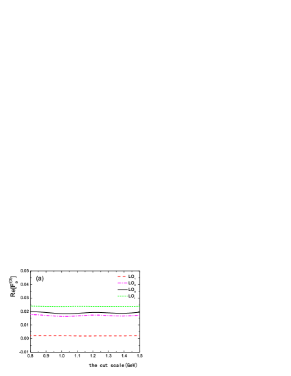
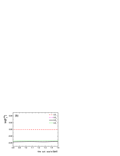
Figure 4: The $\mu_{0}$-dependence of the LO time-like scalar pion form factor $F^{\prime(0)}_{a,I}$ and $F^{\prime(0)}_{a,II}$ on the variations of the cutoff scale $\mu_{0}$ in the range of $0.8\leq\mu_{0}\leq 1.5$ GeV. (a) the real part ${\rm Re}[F^{\prime(0)}_{a}]$, and (b) the imaginary part ${\rm Im}[F^{\prime(0)}_{a}]$. For more details see text.

In the framework of the pQCD factorization approach, we usually choose the lower cutoff scale $\mu_{0}=1$ GeV for the hard scale t in the running of the Wilson coefficients $C_{i}(t)$. In the numerical integrations we will fix the values $C_{i}(t)$ at $C_{i}(\mu_{0})$ whenever the scale $t$ runs below the cutoff scale $\mu_{0}=1$ GeV.

In Fig. 4, we plot the pQCD predictions for the values and $\mu_{0}$-dependence of the real and imaginary part of the LO time-like scalar pion form factor $F^{\prime(0)}_{a,I}$ and $F^{\prime(0)}_{a,II}$, obtained by using the pion DAs as given in Eq. (LABEL:eq:phipi1) and the single-b and double-b convolution respectively. The Fig. 4(a) and 4(b) shows the real and the imaginary part of the form factor, respectively. The dash, dot-dash curve represents the contribution from the 1st, 2nd-term in Eq. (26) respectively; The solid ( dots) line shows the total LO form factor as described in Eq. (26) ( Eq. (28)), when making the double-b (single-b) convolution. From the numerical results as shown in Fig. 4, we find the following points:

1. The second term proportional to $\phi^{P}_{\pi}(x_{2})\phi^{A}_{\pi}(x_{3})$ in Eq. (26) provides the dominant contribution to both the real and imaginary part of the time-like scalar pion form factor, which support our analysis in the paragraph before Eq. (23) and further imply that it’s reasonable to consider the NLO contribution to this dominant term only when we evaluate the NLO corrections to the LO results.

2. The real (imaginary) part of the form factor obtained from the single-b convolution is a bit larger (smaller) than that obtained from the double-b convolution method. But one can see from Fig. 4 that the difference between the pQCD predictions obtained by using the single-b or double-b convolution method is very small in deed. Such similarity can be understood by the fact that the internal gluon propagator provide the major contribution to the imaginary part and the strong phase in the factorizable annihilation diagrams.

3. It is easy to see from Fig. 4 that the pQCD predictions for the LO time-like scalar pion form factor $F^{\prime(0)}_{a,I}$ and $F^{\prime(0)}_{a,II}$ do have a very weak dependence on the value of $\mu_{0}$, this is indeed what we expect.

By comparing the hard kernels as given in Eqs. (12,21), it is easy to find that one can obtain the time-like hard kernel $H^{\prime(0)}_{a}$ from the space-like one $H^{(0)}_{a}$ by simple replacements of $x_{2}\rightarrow 1-x_{3}$ and the analytic continuation $Q^{2}\rightarrow-M^{2}_{B}$. Such connections are also valid for $H^{\prime(0)}_{b}$ and $H^{(0)}_{b}$. So the NLO contribution to the LO time-like scalar hard kernel can also be obtained from the NLO correction to the LO space-like result by the same kinds of replacements and analytical continuations, which will be presented in the next section.

III NLO correction for the space-like scalar pion form factor

In this section we will calculate the ${{\cal O}}(\alpha^{2}_{s})$ quark level diagrams as well as the convolutions of the effective diagrams for the ${{\cal O}}(\alpha_{s})$ wave functions and the LO (${{\cal O}}(\alpha_{s})$) hard kernel in the ’t Hooft-Feynman gauge, and try to find the IR finite NLO corrections to the space-like scalar pion form factor in the $k_{\rm T}$ factorization theorem. From the discussions in last section, we get to know that it is reasonable for us to calculate the NLO corrections to $H^{(0)}_{a,1}$ only, which is the the first term of the LO hard kernel $H^{(0)}_{a}(x_{2},x_{3},Q^{2})$ in Eq. (12), i.e.,

$$H^{(0)}_{a,1}(x_{2},k_{\rm 2T};x_{3},k_{\rm 3T};Q^{2})=\frac{16\pi\alpha_{s}C_{F}m_{0\pi}Q^{2}}{(p_{3}-k_{2})^{2}(k_{2}-k_{3})^{2}}\;\phi^{A}_{\pi}(x_{2})\phi^{P}_{\pi}(x_{3}).$$ (31)

Under the hierarchy as shown in Eq. (6), only those terms which don’t vanish in the limits of $x_{i}\to 0$ and $k_{iT}\to 0$ should be kept.

III.1 NLO contributions of the QCD quark diagrams

We first calculate the NLO (${{\cal O}}(\alpha^{2}_{s})$) corrections to Fig. 1(a) in the $k_{\rm T}$ factorization theorem in this subsection. These NLO corrections include the self-energy diagrams, the vertex diagrams, the box and pentagon diagrams, as illustrated in Figs. (5,6,7) respectively. We will use the dimensional reduction schemeplb84-193 to extract the ultraviolet (UV) divergences, and use the transverse momentum for the external light quarks in Eq. (32) to regulate the IR divergences in loops. Following the method used in Refs. prd83-054029 ; prd89-054015 we make the same definitions for $\delta_{2},\delta_{3}$ and $\delta_{23}$:

$$\delta_{2}=\frac{k^{2}_{2T}}{Q^{2}},\quad\delta_{3}=\frac{k^{2}_{3T}}{Q^{2}},\quad\delta_{23}=\frac{-(k_{2}-k_{3})^{2}}{Q^{2}}.$$ (32)

Figure 5: The self-energy corrections to Fig.1(a).

Following the standard procedure we calculate the one loop self-energy Feynman diagrams as shown in Fig. 5 and find the following NLO self-enegy corrections:

$$G^{(1)}_{5a}=-\frac{\alpha_{s}C_{F}}{8\pi}\left[\frac{1}{\epsilon}+\ln{\frac{4\pi\mu^{2}}{\delta_{2}Q^{2}e^{\gamma_{E}}}}+2\right]H^{(0)},$$

$$G^{(1)}_{5b}=-\frac{\alpha_{s}C_{F}}{8\pi}\left[\frac{1}{\epsilon}+\ln{\frac{4\pi\mu^{2}}{\delta_{2}Q^{2}e^{\gamma_{E}}}}+2\right]H^{(0)},$$

$$G^{(1)}_{5c}=-\frac{\alpha_{s}C_{F}}{8\pi}\left[\frac{1}{\epsilon}+\ln{\frac{4\pi\mu^{2}}{\delta_{3}Q^{2}e^{\gamma_{E}}}}+2\right]H^{(0)},$$

$$G^{(1)}_{5d}=-\frac{\alpha_{s}C_{F}}{8\pi}\left[\frac{1}{\epsilon}+\ln{\frac{4\pi\mu^{2}}{\delta_{3}Q^{2}e^{\gamma_{E}}}}+2\right]H^{(0)},$$

$$G^{(1)}_{5e}=-\frac{\alpha_{s}C_{F}}{4\pi}\left[\frac{1}{\epsilon}+\ln{\frac{4\pi\mu^{2}}{x_{2}Q^{2}e^{\gamma_{E}}}}+2\right]H^{(0)},$$

$$G^{(1)}_{5f+5g+5h+5i}=\frac{\alpha_{s}}{4\pi}\left[\left(5-\frac{2}{3}N_{f}\right)\left(\frac{1}{\epsilon}+\ln{\frac{4\pi\mu^{2}}{\delta_{23}Q^{2}e^{\gamma_{E}}}}\right)\right]H^{(0)},$$ (33)

where $1/\epsilon$ represents the UV pole term, $\mu$ is the renormalization scale,$\gamma_{E}$ is the Euler constant, $N_{f}$ is the number of the active quarks flavors, and $H^{(0)}=H^{(0)}_{a,1}(x_{2},k_{\rm 2T};x_{3},k_{\rm 3T};Q^{2})$ has been defined in Eq. (31). For the sake of simplicity, we will use the abbreviation $H^{(0)}$ instead of the term $H^{(0)}_{a,1}(x_{2},k_{\rm 2T};x_{3},k_{\rm 3T};Q^{2})$ to denote the LO hard kernel throughout the text unless otherwise stated explicitly. The Figs. 5(f,g,h,i) denote the self-energy corrections to the exchanged gluon itself.

It’s easy to find that all these self energy corrections are equal to the self energy corrections for the pion electromagnetic form factorsprd83-054029 ; prd89-054015 , because these self energy diagrams just correct the light quark fields, while don’t involve the inner structure of the initial and final mesons. The additional factor $1/2$ is considered for self energy diagrams Fig. 5(a,b,c,d) because of the freedom to choose the most outside vertex of the radiative gluon.

Figure 6: The vertex corrections to Fig.1(a).

The vertex correction diagrams with three-point loop integrals are plotted in Fig. 6, the NLO corrections from these five vertex diagrams are summarized in the following form:

$$G^{(1)}_{6a} = \frac{\alpha_{s}C_{F}}{4\pi}\left[\frac{1}{\epsilon}+\ln{\frac{4\pi\mu^{2}}{Q^{2}e^{\gamma_{E}}}}-2\ln{x_{2}}\ln{\delta_{2}}-2\ln{\delta_{2}}-2\ln{x_{2}}-\frac{5\pi^{2}}{2}+2\right]H^{(0)},$$

$$G^{(1)}_{6b} = -\frac{\alpha_{s}}{8\pi N_{c}}\left[\frac{1}{\epsilon}+\ln{\frac{4\pi\mu^{2}}{x_{2}Q^{2}e^{\gamma_{E}}}}+1\right]H^{(0)},$$

$$G^{(1)}_{6c} = -\frac{\alpha_{s}}{8\pi N_{c}}\left[\frac{1}{\epsilon}+\ln{\frac{4\pi\mu^{2}}{\delta_{23}Q^{2}e^{\gamma_{E}}}}-\ln{\frac{\delta_{2}}{\delta_{23}}}\ln{\frac{\delta_{3}}{\delta_{23}}}-\ln{\frac{\delta_{3}}{\delta_{23}}}-\ln{\frac{\delta_{3}}{\delta_{23}}}-\frac{\pi^{2}}{3}+2\right]H^{(0)},$$

$$G^{(1)}_{6d} = \frac{\alpha_{s}N_{c}}{8\pi}\left[\frac{3}{\epsilon}+3\ln{\frac{4\pi\mu^{2}}{\delta_{23}Q^{2}e^{\gamma_{E}}}}-\ln{\frac{\delta_{2}}{\delta_{23}}}-\ln{\frac{\delta_{3}}{\delta_{23}}}+6\right]H^{(0)},$$

$$G^{(1)}_{6e} = \frac{\alpha_{s}N_{c}}{8\pi}\left[\frac{3}{\epsilon}+3\ln{\frac{4\pi\mu^{2}}{x_{2}Q^{2}e^{\gamma_{E}}}}-\ln{x_{3}}\ln{\delta_{3}}-\ln{\delta_{3}}\right.$$ (34)

$$\left.+\ln{x_{2}}\ln{x_{3}}+\ln{x_{3}}-\frac{\pi^{2}}{3}+6\right]H^{(0)}.$$

All these five vertex diagrams would have IR divergences at the first sight. The radiated gluon in Fig. 6(a) would generate the collinear divergence when it’s parallel to the initial momentum $p_{2}$. Fig. 6(b) would include the collinear divergence at $l\parallel p_{3}$ region. Fig. 6(c) would generate both the soft and collinear divergence because the radiated gluon is attached to the external light quark lines, then the double logarithm would appear. The radiated gluon in Fig. 6(d) would generate the collinear divergences from $l\parallel p_{2}$ and $l\parallel p_{3}$ regions, while the gluon in Fig. 6(e) could generate the collinear divergence in the $l\parallel p_{2}$ region. But the detailed calculations show that the collinear singularity in Fig. 6(b) is forbidden by the kinetics, so $G^{(1)}_{6b}$ is IR finite.

The box and pentagon diagram in Fig. 7 are more complicate because they would involve four-point and five-point integrals. But the sub-diagrams Figs. 7(a,e) are reducible diagrams and their contributions will be canceled completely by the relevant effective diagrams to be evaluated in the next subsection, so we can set them to be zero here safely. Then we just need to calculate three four-point diagrams Figs. 7(b,d,f) and one five-point diagram Fig. 7(c). From the evaluations of the Feynman diagrams in Fig. 7 we find the following NLO corrections:

$$G^{(1)}_{7a,7e} \equiv 0,$$

$$G^{(1)}_{7b} = -\frac{\alpha_{s}N_{c}}{8\pi}\left[\ln{\delta_{2}}-\ln{\delta_{23}}-1\right]H^{(0)},$$

$$G^{(1)}_{7c} = -\frac{\alpha_{s}}{8\pi N_{c}}\left[\ln{\delta_{2}}\ln{\delta_{3}}-2\ln{x_{2}}\ln{\delta_{2}}-\ln{\delta_{2}}+\frac{1}{2}\ln^{2}{\delta_{23}}-\ln^{2}{x_{3}}-\frac{5}{12}\pi^{2}\right]H^{(0)},$$

$$G^{(1)}_{7d} = \frac{\alpha_{s}}{8\pi N_{c}}\left[\ln{\delta_{2}}\ln{\delta_{3}}-2\ln{x_{2}}\ln{\delta_{2}}+\ln{\delta_{3}}-\ln{x_{2}}-\frac{\pi^{2}}{3}-1\right]H^{(0)},$$

$$G^{(1)}_{7f} = -\frac{\alpha_{s}}{8\pi N_{c}}\left[\ln{\frac{\delta_{1}}{\delta_{23}}}\ln{\frac{\delta_{3}}{\delta_{23}}}-\ln{x_{3}}\ln{\delta_{3}}+\frac{1}{2}\ln^{2}{\delta_{23}}\right.$$ (35)

$$\left.+\ln{x_{2}}\ln{x_{3}}-\frac{3}{2}\ln^{2}{x_{3}}-\frac{\pi^{2}}{3}-1\right]H^{(0)}.$$

The three sub-diagrams Figs. 7(c,d,f) all generate the double logarithms, because the two end-points of the radiated gluon is attached to the external lines, which could result in the soft and collinear singularities. The Fig. 7(b) contains only the collinear divergence in the $l\parallel p_{2}$ region because one end-point of the radiated gluon is attached to the internal gluon.

For the remaining IR singularities generated in Figs. (5,6,7), we can sort them into two groups as shown in Eqs. (36,37) by using the phase space splicing method prd65-094032 : one is from the region $l\parallel p_{2}$ and the other is from the region $l\parallel p_{3}$.

$$G^{(1)}_{\rm IR1} = \frac{\alpha_{s}C_{F}}{4\pi}\left[-2\ln{x_{2}}\ln{\delta_{2}}-4\ln{\delta_{2}}\right]H^{(0)},$$ (36)

$$G^{(1)}_{\rm IR2} = \frac{\alpha_{s}C_{F}}{8\pi}\left[-2\ln{x_{3}}\ln{\delta_{3}}-4\ln{\delta_{3}}\right]H^{(0)}.$$ (37)

Figure 7: The Box and pentagon corrections to Fig.1(a).

As for the UV divergences, they are forbidden for the Feynman diagrams in Fig. 7 from the surface divergence analysis. The UV divergences in the NLO quark level diagrams in Figs. (5,6) can be summed up and written in the form of

$$\frac{\alpha_{s}}{4\pi}\left(11-\frac{2}{3}N_{f}\right)\frac{1}{\epsilon}.$$ (38)

Such UV divergence is the same one as that appeared in the pion electromagnetic form factors prd83-054029 ; prd89-054015 .

III.2 Convolutions of the NLO Wave Functions With the LO Hard Kernel

As argued in Refs. prd64-014019 ; prd67-034001 ; epjc40-395 ; prd89-054015 , the IR divergences of the NLO corrections from the quark level Feynman diagrams in Figs. (5,6,7) can be absorbed into the non-perturbative wave functions which are universal. Based on this argument, we will make a convolution of the NLO wave functions with the LO hard kernel $H^{(0)}$, and find that the resultant IR part should cancel the IR divergences appeared in the NLO amplitude $G^{(1)}_{\rm IR1}$ and $G^{(1)}_{\rm IR2}$ as given in Eqs. (36,37). The twist-2 part of the initial pion wave function $\Phi_{\pi,A}(x_{2},k_{2T};x^{\prime}_{2},k^{\prime}_{2T})$ and the twist-3 part of the final state pion wave function $\Phi_{\pi,P}(x^{\prime}_{3},k^{\prime}_{3T};x_{3},k_{3T})$ can be defined by the non-local matrix elements prd64-014019 ; prd67-034001 ; epjc40-395 ; prd89-054015 ,

$$\Phi_{\pi,A}(x_{2},k_{2T};x^{\prime}_{2},k^{\prime}_{2T}) = \int\frac{dy^{-}}{2\pi}\frac{d^{2}y_{T}}{(2\pi)^{2}}e^{-ix^{\prime}_{2}P^{+}_{2}y^{-}+i\textbf{k}^{\prime}_{2T}\cdot\textbf{y}_{T}}$$ (39)

$$\cdot<0\mid\overline{q}(y)\gamma_{5}n/_{-}W_{y}(n_{1})^{{\dagger}}I_{n_{1};y,0}W_{0}(n_{1})q(0)\mid\overline{u}(P_{2}-k_{2})d(k_{2})>,$$

$$\Phi_{\pi,P}(x^{\prime}_{3},k^{\prime}_{3T};x_{3},k_{3T}) = \int\frac{dz^{+}}{2\pi}\frac{d^{2}z_{T}}{(2\pi)^{2}}e^{-ix^{\prime}_{3}P^{-}_{3}z^{+}+i\textbf{k}^{\prime}_{3T}\cdot\textbf{z}_{T}}$$ (40)

$$\cdot<0\mid\overline{q}(z)W_{z}(n_{2})^{{\dagger}}I_{n_{2};z,0}W_{0}(n_{2})\gamma_{5}q(0)\mid u(P_{3}-k_{3})\overline{d}(k_{3})>,$$

where $y=(0,y^{-},\textbf{y}_{T})$ and $z=(z_{+},0,\textbf{z}_{T})$ are the light-cone coordinates of the anti-quark field $\bar{q}$, $W_{y}(n_{1})$ and $W_{y}(n_{2})$ with the choice of $n^{2}_{i}\neq 0$ to avoid the light-cone singularityprd85-074004 ; jhep0601-067 ; liLC2014 are the Wilson line integrals:

$$W_{y}(n_{1}) = {\cal P}\;\exp[-ig_{s}\int^{\infty}_{0}d\lambda n_{1}\cdot A(y+\lambda n_{1})],$$ (41)

$$W_{z}(n_{2}) = {\cal P}\;\exp[-ig_{s}\int^{\infty}_{0}d\lambda n_{2}\cdot A(z+\lambda n_{2})],$$ (42)

where the symbol ${\cal P}$ denotes the path ordering operator.

Figure 8: The effective $O(\alpha_{s})$ diagrams for the twist-2 initial $\pi$ meson wave functions.

We firstly consider the convolutions of the ${\cal O}(\alpha_{s})$ twist-2 initial pion wave functions $\Phi^{(1)}_{\pi,A,i}$, as shown in Fig. 8, with the ${\cal O}(\alpha_{s})$ hard kernel $H^{(0)}$ in Eq. (31),

$$\Phi^{(1)}_{\pi,A}\otimes H^{(0)}\equiv\sum^{h}_{i=a}\int dx^{\prime}_{2}d^{2}\textbf{k}^{\prime}_{2T}\Phi^{(1)}_{\pi,A,i}(x_{2},\textbf{k}_{2T};x^{\prime}_{2},\textbf{k}^{\prime}_{2T})H^{(0)}(x^{\prime}_{2},\textbf{k}^{\prime}_{2T};x_{3},\textbf{k}_{3T}).$$ (43)

The reducible effective diagram Fig. 8(c) carry all the NLO contributions from the reducible diagrams Fig. 7(a), so we can also set it’s contribution to be zero safely. The convolutions of the NLO initial wave functions $\Phi^{(1)}_{\pi,A,i}$ and the LO hard kernel $H^{(0)}$ are summarized as

$$\Phi^{(1)}_{\pi,A,a}\otimes H^{(0)}=-\frac{\alpha_{s}C_{F}}{8\pi}\left[\frac{1}{\epsilon}+\ln{\frac{4\pi\mu^{2}_{f}}{\delta_{2}Q^{2}e^{\gamma_{E}}}}+2\right]H^{(0)},$$

$$\Phi^{(1)}_{\pi,A,b}\otimes H^{(0)}=-\frac{\alpha_{s}C_{F}}{8\pi}\left[\frac{1}{\epsilon}+\ln{\frac{4\pi\mu^{2}_{f}}{\delta_{2}Q^{2}e^{\gamma_{E}}}}+2\right]H^{(0)},$$

$$\Phi^{(1)}_{\pi,A,c}\otimes H^{(0)}\equiv 0,$$

$$\Phi^{(1)}_{\pi,A,d}\otimes H^{(0)}=\frac{\alpha_{s}C_{F}}{4\pi}\left[\frac{1}{\epsilon}+\ln{\frac{4\pi\mu^{2}_{f}}{\xi^{2}_{2}e^{\gamma_{E}}}}-\ln^{2}{(\delta_{2}r_{Q2})}-2\ln{(\delta_{2}r_{Q2})}-\frac{\pi^{2}}{3}+2\right]H^{(0)},$$

$$\Phi^{(1)}_{\pi,A,e}\otimes H^{(0)}=\frac{\alpha_{s}C_{F}}{4\pi}\left[\ln^{2}{(\frac{\delta_{2}r_{Q2}}{x_{2}})}+\pi^{2}\right]H^{(0)},$$

$$\Phi^{(1)}_{\pi,A,f}\otimes H^{(0)}=\frac{\alpha_{s}C_{F}}{4\pi}\left[\frac{1}{\epsilon}+\ln{\frac{4\pi\mu^{2}_{f}}{\xi^{2}_{2}e^{\gamma_{E}}}}-\ln^{2}{(\frac{\delta_{2}r_{Q2}}{x^{2}_{2}})}-2\ln{(\frac{\delta_{2}r_{Q2}}{x^{2}_{2}})}-\frac{\pi^{2}}{3}+2\right]H^{(0)},$$

$$\Phi^{(1)}_{\pi,A,g}\otimes H^{(0)}=\frac{\alpha_{s}C_{F}}{4\pi}\left[\ln^{2}{(\frac{\delta_{2}r_{Q2}}{x^{2}_{2}})}-\frac{\pi^{2}}{3}\right]H^{(0)},$$

$$(\Phi^{(1)}_{\pi,A,h}+\Phi^{(1)}_{\pi,A,i}+\Phi^{(1)}_{\pi,A,j})\otimes H^{(0)}=\frac{\alpha_{s}C_{F}}{2\pi}\left[\frac{1}{\epsilon}+\ln{\frac{4\pi\mu^{2}_{f}}{Q^{2}e^{\gamma_{E}}}}-\ln{\delta_{23}}\right]H^{(0)},$$ (44)

where $r_{Q2}=Q^{2}/\xi^{2}_{2}$ and the scale $\xi^{2}_{2}\equiv 4(n_{1}\cdot p_{2})^{2}/|n^{2}_{1}|=Q^{2}|n^{-}_{1}/n^{+}_{1}|$ are introduced to regularize the light corn singularity. We can find that the double logarithms only generated from the effective diagrams without the loop momentum $l$ flowing into the LO hard kernel, such as the case in Figs. 8(d) and 8(f), because the effective diagrams with the soft loop momentum flowing into the LO hard kernel are highly suppressed by the dynamics. These double logarithms are canceled each other completely, resulting in single logarithms only. These single logarithms will be canceled by the IR singularity as given in Eq. (36) from the NLO quark level diagrams.

Figure 9: The effective $O(\alpha_{s})$ diagrams for the twist-3 final $\pi$ meson wave functions.

The remaining convolutions to be treated are those between the ${\cal O}(\alpha_{s})$ hard kernel $H^{(0)}$ and the ${\cal O}(\alpha_{s})$ twist-3 final state pion wave functions $\Phi^{(1)}_{\pi,P,i}$ as shown in Fig. 9.

$$H^{(0)}\otimes\Phi^{(1)}_{\pi,P}\equiv\sum^{h}_{i=a}\int dx^{\prime}_{3}d^{2}3\textbf{k}^{\prime}_{3T}H^{(0)}(x_{2},\textbf{k}_{2T};x^{\prime}_{3},\textbf{k}^{\prime}_{3T})\Phi^{(1)}_{\pi,P,i}(x^{\prime}_{3},\textbf{k}^{\prime}_{3T};x_{3},\textbf{k}_{3T}).$$ (45)

We can also set the convolution of the $H^{(0)}$ and Fig. 9(c) zero with the same reason as for the Fig. 8(c). Then all the convolutions of the effective diagrams in Fig. 9 read as

$$H^{(0)}\otimes\Phi^{(1)}_{\pi,P,a}=-\frac{\alpha_{s}C_{F}}{8\pi}\left[\frac{1}{\epsilon}+\ln{\frac{4\pi\mu^{2}_{f}}{\delta_{3}Q^{2}e^{\gamma_{E}}}}+2\right]H^{(0)},$$

$$H^{(0)}\otimes\Phi^{(1)}_{\pi,P,b}=-\frac{\alpha_{s}C_{F}}{8\pi}\left[\frac{1}{\epsilon}+\ln{\frac{4\pi\mu^{2}_{f}}{\delta_{3}Q^{2}e^{\gamma_{E}}}}+2\right]H^{(0)},$$

$$H^{(0)}\otimes\Phi^{(1)}_{\pi,P,c}\equiv 0,$$

$$H^{(0)}\otimes\Phi^{(1)}_{\pi,P,d}=\frac{\alpha_{s}C_{F}}{8\pi}\left[\frac{1}{\epsilon}+\ln{\frac{4\pi\mu^{2}_{f}}{\xi^{2}_{3}e^{\gamma_{E}}}}-\ln^{2}{(\delta_{3}r_{Q3})}-2\ln{(\delta_{3}r_{Q3})}-\frac{\pi^{2}}{3}+2\right]H^{(0)},$$

$$H^{(0)}\otimes\Phi^{(1)}_{\pi,P,e}=\frac{\alpha_{s}C_{F}}{8\pi}\left[\ln^{2}{(\frac{\delta_{3}r_{Q3}}{x_{3}})}+\pi^{2}\right]H^{(0)},$$

$$H^{(0)}\otimes\Phi^{(1)}_{\pi,P,f}=\frac{\alpha_{s}C_{F}}{8\pi}\left[\frac{1}{\epsilon}+\ln{\frac{4\pi\mu^{2}_{f}}{\xi^{2}_{3}e^{\gamma_{E}}}}-\ln^{2}{(\frac{\delta_{3}r_{Q3}}{x^{2}_{3}})}-2\ln{(\frac{\delta_{3}r_{Q3}}{x^{2}_{3}})}-\frac{\pi^{2}}{3}+2\right]H^{(0)},$$

$$H^{(0)}\otimes\Phi^{(1)}_{\pi,P,g}=\frac{\alpha_{s}C_{F}}{8\pi}\left[\ln^{2}{(\frac{\delta_{3}r_{Q3}}{x^{2}_{3}})}-\frac{\pi^{2}}{3}\right]H^{(0)},$$

$$H^{(0)}\otimes(\Phi^{(1)}_{\pi,P,h}+\Phi^{(1)}_{\pi,P,i}+\Phi^{(1)}_{\pi,P,j})=\frac{\alpha_{s}C_{F}}{4\pi}\left[\frac{1}{\epsilon}+\ln{\frac{4\pi\mu^{2}_{f}}{Q^{2}e^{\gamma_{E}}}}-\ln{\delta_{23}}\right]H^{(0)},$$ (46)

where $r_{Q3}=Q^{2}/\xi^{2}_{3}$ with the scale $\xi^{2}_{3}\equiv 4(n_{2}\cdot p_{3})^{2}/|n^{2}_{2}|=Q^{2}|n^{+}_{2}/n^{-}_{2}|$. The double logarithms in Eq. (46) are also canceled each other as the case in Eq. (44), and the remaining single logarithms can also been canceled by the IR singularity in Eq. (37). When compared with the convolutions of the irreducible diagrams in Figs. 8(d,e,f,g), there is an additional factor $1/2$ for those of the irreducible diagrams Fig. 9(d,e,f,g), since the twist-3 final state wave functions $\Phi^{(1)}_{\pi,P,i}$ have different spin structure from the twist-2 initial state wave function $\Phi^{(1)}_{\pi,A,i}$.

III.3 The NLO Hard Kernel

The $k_{\rm T}$ factorization theorem states that the NLO hard kernel can be obtained by taking the difference of the NLO quark level diagrams and the convolutions of LO hard kernel with NLO wave functions prd64-014019 ; prd67-034001 ; epjc40-395 ; prd89-054015 , i.e.,

$$H^{(1)}(x_{2},\textbf{k}_{2T};x_{3},\textbf{k}_{3T})=G^{(1)}(x_{2},\textbf{k}_{2T};x_{3},\textbf{k}_{3T})$$

$$~{}~{}~{}~{}~{}~{}~{}~{}~{}~{}~{}~{}~{}~{}-\sum^{h}_{i=a}\int dx^{\prime}_{2}d^{2}\textbf{k}^{\prime}_{2T}\Phi^{(1)}_{\pi,A,i}(x_{2},\textbf{k}_{2T};x^{\prime}_{2},\textbf{k}^{\prime}_{2T})H^{(0)}(x^{\prime}_{2},\textbf{k}^{\prime}_{2T};x_{3},\textbf{k}_{3T})$$

$$~{}~{}~{}~{}~{}~{}~{}~{}~{}~{}~{}~{}~{}~{}-\sum^{h}_{i=a}\int dx^{\prime}_{3}d^{2}\textbf{k}^{\prime}_{3T}H^{(0)}(x_{2},\textbf{k}_{2T};x^{\prime}_{3},\textbf{k}^{\prime}_{3T})\Phi^{(1)}_{\pi,P,i}(x^{\prime}_{3},\textbf{k}^{\prime}_{3T};x_{3},\textbf{k}_{3T}).$$ (47)

Besides the contributions from the reducible diagrams, we here sum up all $G^{(1)}_{i}$ as given in Eqs. (33,34,35) to obtain the NLO corrections $G^{(1)}$ from the quark level diagrams in Figs. (5,6,7) for $N_{f}=6$ and find the result,

$$G^{(1)} = \frac{\alpha_{s}C_{F}}{8\pi}\Biggl{[}\frac{29}{2}\left(\frac{1}{\epsilon}+\ln{\frac{4\pi\mu^{2}}{Q^{2}e^{\gamma_{E}}}}\right)-4\ln{\delta_{2}(\ln{x_{2}}+1)-2\ln{\delta_{3}}}(\ln{x_{3}}+1)-\frac{1}{4}\ln^{2}{\delta_{23}}$$

$$+\frac{9}{4}\ln{\delta_{23}}+\frac{1}{2}\ln{x_{2}}\ln{x_{3}}+\frac{5}{8}\ln^{2}{x_{3}}-\frac{43}{4}\ln{x_{2}}+\frac{9}{4}\ln{x_{3}}-\frac{267\pi^{2}}{48}+\frac{65}{2}\Biggr{]}H^{(0)}.$$

By summing up all convolutions as listed in Eqs. (44,46) for Figs. (8,9) without the reducible diagrams, we find the total result:

$$\Phi^{(1)}_{\pi,A}\otimes H^{(0)} = \frac{\alpha_{s}C_{F}}{4\pi}\Bigl{[}\frac{4}{\epsilon}+4\ln{\frac{4\pi}{e^{\gamma_{E}}}}+4\ln{\frac{\mu^{2}_{f}}{Q^{2}}}-2\ln{(\delta_{2}r_{Q2})}(\ln{x_{2}}+2)$$ (49)

$$+\ln^{2}{x_{2}}-2\ln{\delta_{23}}+4\ln{(x_{2}r_{Q2})}-\pi^{2}+4\Bigr{]}H^{(0)},$$

$$H^{(0)}\otimes\Phi^{(1)}_{\pi,P} = \frac{\alpha_{s}C_{F}}{8\pi}\Bigl{[}\frac{4}{\epsilon}+4\ln{\frac{4\pi}{e^{\gamma_{E}}}}+4\ln{\frac{\mu^{2}_{f}}{Q^{2}}}-2\ln{(\delta_{3}r_{Q3})}(\ln{x_{3}}+2)$$ (50)

$$+\ln^{2}{x_{3}}-2\ln{\delta_{23}}+4\ln{(x_{3}r_{Q3})}-\pi^{2}+4\Bigr{]}H^{(0)}.$$

The UV divergence in Eq. (LABEL:eq:nloqd), which would determine the renormalization-group (RG) evolution of the strong coupling constant $\alpha_{s}$, is the same one as that in the pion electromagnetic form factor as given in Refs. prd83-054029 ; prd89-054015 . The bare coupling constant $\alpha_{s}$ in Eqs. (LABEL:eq:nloqd,49,50) can be rewritten as

$$\alpha_{s}=\alpha_{s}(\mu_{f})+\delta Z(\mu_{f})\alpha_{s}(\mu_{f}),$$ (51)

with the counter-term $\delta Z(\mu_{f})$ defined in the modified minimal subtraction scheme($\overline{MS}$). We can insert the $\alpha_{s}$ in Eq. (51) into Eqs. (31,LABEL:eq:nloqd,49,50) to regularize the UV poles in Eq. (47) through the term $\delta Z(\mu_{f})H^{(0)}$, and then the UV poles in Eqs. (49,50) are regulated by the counter-term of the quark field and by an additional counter-term in Eq. (51).

One should be careful that the internal quark with the tiny momentum fraction $x_{2}$ would be on-shell, which would then generate an additional double logarithm $\ln^{2}{x_{2}}$, so we must subtract this jet function as described in Eq. (52) to obtain the real NLO hard kernel.

$$J^{(1)}H^{(0)} = -\frac{1}{2}\frac{\alpha_{s}(\mu_{f})C_{F}}{4\pi}\left[\ln^{2}{x_{2}}+\ln{x_{2}}+\frac{\pi^{2}}{3}\right]H^{(0)}.$$ (52)

After renormalizing the UV divergences and subtracting the jet function, one can obtain the NLO hard kernel for Fig. 1(a) by combing the results as given previously in Eqs. (47,LABEL:eq:nloqd,49,50) together:

$$H^{(1)}(x_{i},\mu,\mu_{f},Q^{2}) \equiv F^{(1)}(x_{i},\mu,\mu_{f},Q^{2})H^{(0)},$$ (53)

with

$$F^{(1)}(x_{i},\mu,\mu_{f},Q^{2}) = \frac{\alpha_{s}(\mu_{f})C_{F}}{8\pi}\Biggl{[}\frac{21}{2}\ln{\frac{\mu^{2}}{Q^{2}}}-8\ln{\frac{\mu^{2}_{f}}{Q^{2}}}-\frac{1}{4}\ln^{2}{\delta_{23}}+\frac{33}{4}\ln{\delta_{23}}+\frac{1}{2}\ln{x_{2}}\ln{x_{3}}$$ (54)

$$-\frac{3}{8}\ln^{2}{x_{3}}-\ln^{2}{x_{2}}-\frac{71}{4}\ln{x_{2}}-\frac{7}{4}\ln{x_{3}}-\frac{107}{48}\pi^{2}+\frac{41}{2}\Biggr{]},$$

here one has made the choice for $r_{Q2}=r_{Q3}\equiv 1$ as in Refs. prd83-054029 ; prd89-054015 .

III.4 Numerical results and discussions

In this subsection we will calculate the NLO corrections to the space-like scalar pion form factor in the $k_{T}$ factorization theorem numerically. From the expression of the NLO hard kernel $H^{(1)}(x_{i},\mu,\mu_{f},Q^{2})$ as given in Eq. (53), one can define the space-like scalar pion form factor for Fig. 1(a) up to NLO as the form of

$$Q^{2}F(Q^{2})| {}_{\rm NLO}=8\pi m_{0\pi}C_{F}Q^{4}\int{dx_{2}dx_{3}}\int{b_{2}db_{2}b_{3}db_{3}}~{}\alpha_{s}(t)\cdot e^{-2S_{\pi}(t)}\cdot h(x_{2},x_{3},b_{2},b_{3})$$

$$\cdot\Bigl{\{}2\phi^{A}_{\pi}(x_{2})\phi^{P}_{\pi}(x_{3})S_{t}(x_{3})\left[1+F^{(1)}(x_{i},\mu,\mu_{f},Q^{2})\right]+x_{2}\left[\phi^{P}_{\pi}(x_{2})-\phi^{T}_{\pi}(x_{3})\right]\phi^{A}_{\pi}(x_{3})\Bigr{\}},$$

where the function $F^{(1)}(x_{i},\mu,\mu_{f},Q^{2})$ describes the NLO contribution to the space-like scalar pion form factor and has been defined in Eq. (54).

Since the initial and final state meson are the same pion meson, which is a $q\bar{q}$ bound state and also a Nambu-Goldstone boson, then there is an exchange symmetry of the momentum fractions for the two sub-diagrams in Fig. 1, as we have demonstrated in Section. II. This symmetry imply that the NLO correction $F^{(1)}_{b}(x_{i},\mu,\mu_{f},Q^{2})$ to the dominant first term proportional to $\phi^{A}_{\pi}(x_{3})\phi^{P}_{\pi}(x_{2})$ in $H^{(0)}_{b}(x_{2},x_{3},Q^{2})$ in Eq. (17) can be obtained from $F^{(1)}(x_{i},\mu,\mu_{f},Q^{2})$ in Eq. (54) by simple replacements of $x_{2}\leftrightarrow x_{3}$, and is of the form

$$F^{(1)}_{b}(x_{i},\mu,\mu_{f},Q^{2}) = \frac{\alpha_{s}(\mu_{f})C_{F}}{8\pi}\Biggl{[}\frac{21}{2}\ln{\frac{\mu^{2}}{Q^{2}}}-8\ln{\frac{\mu^{2}_{f}}{Q^{2}}}-\frac{1}{4}\ln^{2}{\delta_{23}}+\frac{33}{4}\ln{\delta_{23}}$$ (56)

$$+\frac{1}{2}\ln{x_{3}}\ln{x_{2}}-\frac{3}{8}\ln^{2}{x_{2}}-\ln^{2}{x_{3}}-\frac{71}{4}\ln{x_{3}}-\frac{7}{4}\ln{x_{2}}-\frac{107}{48}\pi^{2}+\frac{41}{2}\Biggr{]}.$$

while the space-like scalar pion form factor from Fig. 1(b) up to NLO level can be written as the form of

$$Q^{2}F(Q^{2})|_{\rm b,NLO} = 8\pi m_{0\pi}C_{F}Q^{4}\int{dx_{2}dx_{3}}\int{b_{2}db_{2}b_{3}db_{3}}~{}\alpha_{s}(t)\cdot e^{-2S_{\pi}(t)}\cdot h(x_{2},x_{3},b_{2},b_{3})$$

$$\cdot\Bigl{\{}2\phi^{A}_{\pi}(x_{3})\phi^{P}_{\pi}(x_{2})S_{t}(x_{2})\left[1+F^{(1)}_{b}(x_{i},\mu,\mu_{f},Q^{2})\right]+x_{3}\left[\phi^{P}_{\pi}(x_{3})-\phi^{T}_{\pi}(x_{3})\right]\phi^{A}_{\pi}(x_{2})\Bigr{\}}.$$

Explicit analytical calculations also confirmed this exchanging symmetry directly.

Figure 10: The pQCD predictions for the space-like scalar pion form factor $Q^{2}F(Q^{2})$ for Fig. 1(a) and for Fig. 1(b).

In Fig. 10, we plot the $Q^{2}$-dependence of the pQCD predictions for the form factor $Q^{2}F(Q^{2})$. The Fig. 10(a) and Fig. 10(b) shows the result from Fig. 1(a) and Fig. 1(b), respectively. The upper dot-dashed and lower dotted curve shows the LO contribution and the NLO correction respectively, while the solid curve refers to the total pQCD predictions after the inclusion of the NLO corrections. From the numerical results as illustrated in Fig. 10, we find the following points:

1. As shown by the dots line in Fig. 10, the NLO correction to the LO pQCD prediction for $Q^{2}F(Q^{2})$ is negative in sign and very small in magnitude in the whole considered region of $Q^{2}$. The inclusion of the NLO corrections can produce a small decrease, less than $8\%$ in magnitude, to the LO result in the region of $1\leq Q^{2}\leq 30$ GeV².

2. As illustrated by the curves in Fig. 10(a,b), the LO and NLO contributions to the form factor $Q^{2}F(Q^{2})$ from Fig. 1(a) and Fig. 1(b) are indeed identical, which is what we expect based on the exchanging symmetry as discussed in Section II.

IV NLO corrections and effects on $B\to\pi\pi$ decays

In this section we will extend our calculations for the NLO correction to the LO space-like scalar pion form factor to the case in the time-like range by the analytical continuation, and then revisit the puzzled $B\to\pi\pi$ decays with the inclusion of this new NLO correction by employing the pQCD factorization approach.

IV.1 NLO corrections to the time-like scalar pion form factor

With the NLO space-like scalar pion hard kernel in Eq. (54) and the analytical continuation relation, we can obtain the NLO hard amplitude for the time-like scalar pion form factor in the $k_{\rm T}$ space by substituting $-M^{2}_{B}-i\epsilon$ for the scale $Q^{2}$ of the factorizable annihilation process in the B meson decays, and $-x_{2}(1-x_{3})M^{2}_{B}+|{\textbf{k}_{\rm 2T}}-{\textbf{k}_{\rm 3T}}|^{2}-i\epsilon$ for the internal gluon. The single-b convoluted NLO time-like hard kernel can be expressed as

$$H^{\prime(1)}_{a,32}(x_{i},k_{\rm T},t,M^{2}_{B}) \equiv F^{\prime(1)}_{a,32}(x_{i},k_{\rm T},t,M^{2}_{B})\cdot H^{\prime(0)}_{a,32},$$ (58)

$$F^{\prime(1)}_{a,32}(x_{i},k_{\rm T},t,M^{2}_{B}) = \frac{\alpha_{s}(\mu_{f})C_{F}}{8\pi}\Bigl{[}\frac{5}{2}\ln{\frac{\mu^{2}}{M^{2}_{B}}}-\frac{1}{4}\ln^{2}{\delta^{\prime}_{23}}+\frac{33}{4}\ln{\delta^{\prime}_{23}}-\ln^{2}{(1-x_{3})}$$ (59)

$$-\frac{3}{8}\ln^{2}{x_{2}}+\frac{1}{2}\ln{x_{2}}\ln{(1-x_{3})}-\frac{71}{4}\ln{(1-x_{3})}$$

$$-\frac{7}{4}\ln{x_{2}}-\frac{95}{48}\pi^{2}+\frac{41}{2}+i\pi\left(\frac{1}{2}\ln{\delta^{\prime}_{23}}-\frac{23}{4}\right)\Bigr{]},$$

where $H^{\prime(0)}_{a,32}$ has been given in Eq. (23), $H^{\prime(1)}_{a,32}$ and $F^{\prime(1)}_{a,32}$ represent the corresponding NLO time-like scalar hard kernel and the NLO correction factor with the following notation,

$$\ln{\delta^{\prime}_{23}}=\ln{\frac{|{\textbf{k}_{\rm 2T}}-{\textbf{k}_{\rm 3T}}|^{2}-x_{2}(1-x_{3})M^{2}_{B}}{M^{2}_{B}}}+i\pi\cdot\Theta(|{\textbf{k}_{\rm 2T}}-{\textbf{k}_{\rm 3T}}|^{2}-x_{2}(1-x_{3})M^{2}_{B}).$$ (60)

We can then obtain the NLO single-b convolution time-like scalar pion form factor by the Fourier transformation of Eq. (58) from the ${\textbf{k}_{\rm 3T}}$ space to the $b_{3}$ space as well as the integration over the kinematic variables. And the time-like scalar pion form factor up to NLO level can then be written as,

$$F^{\prime(1)}_{\rm a,I} = -\int^{1}_{0}dx_{2}dx_{3}\int^{\infty}_{0}db_{3}~{}\frac{C_{F}M^{2}_{B}m^{\pi}_{0}}{\pi(1-x_{3})}\cdot\Bigl{\{}2\phi_{\pi}^{P}(x_{2})\phi_{\pi}^{A}(x_{3})S_{t}(x_{2})\;K^{\prime\prime(1)}_{0}(z)$$ (61)

$$+\Bigl{[}(1-x_{3})\phi^{A}_{\pi}(x_{2})\left(\phi^{P}_{\pi}(x_{3})+\phi^{T}_{\pi}(x_{3})\right)+2\phi^{P}_{\pi}(x_{2})\phi^{A}_{\pi}(x_{3})\left(1+F^{\prime(1)}_{32}\right)\cdot S_{t}(x_{2})\Bigr{]}\cdot K_{0}(z)\Bigr{\}}$$

$$\cdot\alpha_{s}(\mu)\cdot\exp\left[-S_{I}(x_{2},b_{2};1-x_{3},b_{3};M_{B};\mu)\right],$$

where $z=i\sqrt{(1-x_{3})x_{2}}M_{B}b_{3}$, the definition of the function $K^{\prime\prime(1)}_{0}(z)$ is of the form

$$K^{\prime\prime(1)}_{0}(z)=\left[\frac{\partial^{2}}{\partial{\alpha^{2}}}K^{(1)}_{\alpha}(z)\right]_{\alpha=0},$$ (62)

which comes from the Fourier transformation of $\ln^{2}{(|{\textbf{k}_{\rm 2T}}-{\textbf{k}_{\rm 3T}}|^{2}-x_{2}(1-x_{3})M^{2}_{B}-i\epsilon)}$, and $\alpha$ denotes the order parameter of the modified Hankel function, and it’s magnitude behaves as $|K^{\prime\prime(1)}_{0}(z)|\sim(1/3)\ln^{2}{(z)}|K_{0}(z)|$ when the argument $|z|\rightarrow 0$. The NLO correction factor $F^{\prime(1)}_{32}$ in Eq. (61) is of the form

$$F^{\prime(1)}_{32}(x_{i},b_{3},t,M^{2}_{B}) = \frac{\alpha_{s}(\mu_{f})C_{F}}{8\pi}\left\{\frac{5}{2}\ln{\frac{\mu^{2}}{M^{2}_{B}}}-\frac{1}{16}\ln^{2}{\left(\frac{4x_{2}(1-x_{3})}{M^{2}_{B}b^{2}_{3}}\right)}\right.$$ (63)

$$\left.+(\frac{33}{8}-\frac{\gamma_{E}}{4})\ln{\left(\frac{4x_{2}(1-x_{3})}{M^{2}_{B}b^{2}_{3}}\right)}-\ln^{2}{(1-x_{3})}-\frac{3}{8}\ln^{2}{x_{2}}+\frac{1}{2}\ln{x_{2}}\ln{(1-x_{3})}\right.$$

$$\left.-\frac{71}{4}\ln{(1-x_{3})}-\frac{7}{4}\ln{x_{2}}-\frac{105}{48}\pi^{2}+\frac{41}{2}-\frac{\gamma^{2}_{E}}{4}-\frac{33\gamma_{E}}{4}+i\pi\cdot\left[\frac{5}{2}\right]\right\},$$

where $\gamma_{E}$ is the Euler constant.

IV.2 NLO effects on $B\to\pi\pi$ decays

In this subsection we will firstly show the NLO contributions to the time-like scalar pion form factor $F^{\prime(1)}_{\rm a,I}$ in the $k_{T}$ factorization theorem numerically, and then examine the effects of such NLO contribution on the pQCD predictions for the branching ratios of the rare $B\to\pi\pi$ decays.

Figure 11: The $\mu_{0}$-dependence of the pQCD predictions for the time-like scalar pion form factor $F^{\prime}_{\rm a,I}$ at the LO and NLO level. The left (right ) figure shows the real (imaginary) part of the form factor. The short-dash and solid line shows the pQCD predictions for the form factor $F^{\prime}_{\rm a,I}$ at the LO and the NLO level, respectively.

In the calculations for the LO time-like scalar pion form factor $F^{\prime(0)}_{\rm a}$, we considered the cases for both the single-b and double-b convolution and found that the differences are very small between these two different convolution methods. Consequently, we make the calculation for the NLO form factor $F^{\prime(1)}_{\rm a}$ as given in Eq. (61) by using the single-b convolution only.

In Fig. 11(a) and 11(b), we show the $\mu_{0}$-dependence of the real and imaginary part of the time-like scalar pion form factor $F^{\prime}_{\rm a,I}$ at the LO and NLO level, respectively. The short-dash line in Fig. 4 shows the LO contribution, while the solid line shows the form factor after the inclusion of the NLO contribution.

In Fig. 12(a) and 12(b), however, we show the $\mu_{0}$-dependence of the pQCD predictions for the absolute values and their arguments of the time-like scalar pion form factor $F^{\prime}_{\rm a,I}$ at the LO (the short-dash line) and NLO (the solid line) level, respectively. For fixed $\mu_{0}=1.0$ GeV, we have numerically

$$F^{\prime}_{\rm a,I} = \left\{\begin{array}[]{ll}0.0238-i0.0340,&{\rm LO_{I}},\\ 0.0259-i0.0329,&{\rm NLO_{I}},\\ \end{array}\right.$$ (66)

$$= \left\{\begin{array}[]{ll}0.0415\cdot\exp[-i55.0^{\circ}],&{\rm LO_{I}},\\ 0.0419\cdot\exp[-i51.8^{\circ}],&{\rm NLO_{I}},\\ \end{array}\right.$$ (69)

From Figs. (11,12) and the numerical results in Eq. (69), one can see the following points:

1. The NLO part is indeed very small in size, brings little correction to both the real- and imaginary part of the LO form factor, and is almost independent with the variation of cutoff scale $\mu_{0}$.

2. The real part of the time-like scalar pion form factor is positive, while its imaginary part is negative, which leads to a large strong phase around $-55^{\circ}$ and play an important role in producing large CP violation for $B\to\pi\pi$ decays.

Figure 12: The same as in Fig. 11, but for the $\mu_{0}$-dependence of the absolute value and their argument of the considered form factor $F^{\prime(0)}_{\rm a,I}$ and $F^{\prime(1)}_{\rm a,I}$.

Table 1: The LO and NLO pQCD predictions for the branching rations (in unit of $10^{-6}$) of the three $B\to\pi\pi$ decays. The last column lists the data from Refs.bf-1406 ; petric-201407 . For details, see text.

Channel	LO	NLO0 prd90-014029	NLO	QCDFnpb675	Data
$Br(B^{0}\to\pi^{+}\pi^{-})$	$6.87$	$7.67$	$7.69^{+3.27}_{-2.67}$	$8.9$	$5.11\pm 0.22$
$Br(B^{+}\to\pi^{+}\pi^{0})$	$3.54$	$4.27$	$4.27^{+1.85}_{-1.47}$	$6.0$	$5.38^{+0.35}_{-0.34}$
$Br(B^{0}\to\pi^{0}\pi^{0})$	$0.12$	$0.23$	$0.24^{+0.09}_{-0.07}$	$0.3$	$0.9\pm 0.12$

In the pQCD factorization approach, the NLO contribution to $B\to\pi\pi$ decays from the factorizable annihilation diagrams are described by the time like scalar pion form factor $F^{\prime(1)}_{\rm a,I}$, in other words, it is the NLO ”annihilation correction”. After the inclusion of this new NLO time-like scalar pion form factor in Eq. (61), we recalculate the three rare decays $B\to\pi\pi$ in the pQCD factorization approach by using the pion distribution amplitudes as given in Eq. (LABEL:eq:phipi1). Because this newly known NLO contribution brings only a very small correction to the LO form factor as we have elaborated in previous section, one generally expect that such new NLO contribution to the time-like scalar pion form factor can not change the pQCD predictions for the $B\to\pi\pi$ decays obviously.

In the framework of the pQCD factorization approach, the LO contributions to $B\to\pi\pi$ decays come from the emission diagrams, the hard-spectator diagrams, the factorizable and non-factorizable annihilation diagrams as illustrated in the Fig. 1 of Ref. prd90-014029 . At the NLO level, on the other hand, those currently known NLO contributions to $B\to\pi\pi$ decays include the following pieces from rather different sources:

1. The Wilson coefficients $C_{i}(m_{\rm W})$ and the renormalization group evolution matrix $U(\mu,m_{\rm W},\alpha)$ at the NLO level buras96 , as well as the strong coupling constant $\alpha_{s}(\mu)$ at two-loop level pdg2014 .

2. The NLO contributions from the vertex corrections (VC), the quark-loops (QL), and the chromo-magnetic penguin operator $O_{8g}$ (MP) as given in Refs. prd72-114005 ; npb675 ; o8g2003 .

3. The NLO twist-2 and twist-3 contributions to the form factors of the $B\to\pi$ transition as presented in Refs. prd85-074004 ; prd89-094004 .

4. The NLO contribution to the time-like scalar pion form factor $F^{\prime}_{\rm a,I}$, i.e., the NLO “annihilation correction” to the factorizable annihilation diagrams (see Fig. 2), evaluated firstly in this paper.

The still missing NLO parts in the pQCD approach are those ${\cal O}(\alpha_{s}^{2})$ contributions to the hard spectator diagrams and the non-factorizable annihilation diagrams.

Following the same procedure as in Ref. prd90-014029 , we make the numerical calculations and present the pQCD predictions for the branching ratios of the three $B\to\pi\pi$ decays after the inclusion of all currently known NLO corrections in Table 1. In the third column of Table 1, we list the NLO pQCD predictions for the branching ratios of three decay modes as given in Ref. prd90-014029 , where all known NLO contributions except for the NLO contribution to the factorizable annihilation diagrams calculated in this paper have been taken into account. The numerical results in the fourth column with the label ”NLO”, however, are obtained with the inclusion of all currently known NLO contributions in the pQCD factorization approach. In fifth column, we show the central values of the theoretical predictions based on the QCDF approach npb675 , while the last column lists the data from Refs.bf-1406 ; petric-201407 .

From our analytical and numerical calculations for the pQCD predictions for the branching ratios of the three $B\to\pi\pi$ decays, we have the following observations:

1. The $B^{+}\to\pi^{+}\pi^{0}$ decay do not receive corrections from this new NLO annihilation correction, because the annihilation diagrams do not contribute to $B^{+}\to\pi^{+}\pi^{0}$ decay mode.

2. For $B^{0}\to(\pi^{+}\pi^{-},\pi^{0}\pi^{0})$ decays, the inclusion of the NLO contribution to the factorizable annihilation diagram can produce a very small enhancement to their branching ratios, less than $3\%$ to the LO results. The well-known $\pi\pi$-puzzle can not be interpreted by the inclusion of this very small NLO contribution. This fact, on the other hand, do support the general expectation in the pQCD factorization approachprd87-094003 ; prd90-014029 : the NLO correction to the annihilation diagrams of $B\to PP$ decays are the higher order corrections to the small quantities, and therefore should be very small in magnitude.

For the CP violating asymmetries of the three $B\to\pi\pi$ decays prd90-014029 , the effects due to the inclusion of the newly known NLO annihilation correction $F^{\prime(1)}_{\rm a,I}$ is also very small in size and can be neglected safely.

V Conclusion

In this paper, we made the first calculation for the NLO contribution to the space-like- and time-like scalar pion form factor in the $k_{\rm T}$ factorization theorem, which is in turn the ${\cal O}(\alpha_{s}^{2})$ NLO correction to the factorizable annihilation diagrams for $B\to\pi\pi$ decays. The external light quarks are all set off-shell by $k^{2}_{\rm iT}$ to regulate the IR divergences which would appear in the NLO calculations.

We calculated both the NLO quark-level diagrams and the convolutions of the LO hard kernel $H^{(0)}$ with the NLO wave functions to obtain the NLO space-like hard kernel $H^{(1)}$. Because all quarks in this process are massless, then all the IR divergences in these two type diagrams can be described by the logarithms $\ln^{2}{(k_{\rm iT})}$. The QCD dynamics ensures that the contribution from the radiated soft gluon is highly suppressed by $1/Q^{2}$ in the perturbative theory, our LO and NLO numerical calculations confirmed this point by showing that the double logarithms $\ln^{2}{(k_{\rm iT})}$ generated from the soft kinetic region are canceled completely between the quark-level diagrams and the effective diagrams respectively. We then prove that all the remaining collinear divergences from the quark-level diagrams are also canceled by those from the effective diagrams at NLO level, which is also the basic requirement of the $k_{\rm T}$ factorization theorem.

We made the numerical evaluations for the space-like scalar pion form factor $Q^{2}F(Q^{2})$ up to NLO by using the full pion DA’s in the integration. From the NLO space-like scalar pion form factor, we found the NLO time-like scalar pion form factor $F^{\prime(1)}_{\rm a,I}$ by analytical continuation, which describes the NLO ${\cal O}(\alpha_{s}^{2})$ contribution to the factorizable annihilation diagrams for the considered $B\to\pi\pi$ decays in this paper. By taking the newly known NLO annihilation correction $F^{\prime(1)}_{\rm a,I}$ into account, we recalculate the branching ratios of the three $B\to\pi\pi$ decays with the inclusion of all currently known NLO contributions, and to check the effect of this NLO annihilation correction.

Based on our analytical evaluations and the numerical results, we found the following points:

1. we completed the first analytical calculation for the NLO contribution to the space-like and time-like scalar pion form factor in the $k_{\rm T}$ factorization theorem.

2. There is an exchanging symmetry between the LO hard kernel $H^{(0)}_{a}$ and $H^{(0)}_{b}$: the contribution to the form factor $Q^{2}F(Q^{2})$ from the Fig. 1(a) and Fig. 1(b) are indeed identical.

3. The NLO correction to the space-like scalar pion form factor has an opposite sign with the LO one but is very small in magnitude, can produce at most $10\%$ decrease to $Q^{2}F(Q^{2})$ in the considered $Q^{2}$ region.

4. By making the analytical continuation, we found the NLO time-like scalar pion form factor $F^{\prime(1)}_{\rm a,I}$ from the space-like one, which describes the NLO annihilation correction to the considered $B\to\pi\pi$ decays.

5. The NLO part of the form factor $F^{\prime(1)}_{\rm a,I}$ is very small in size, and is almost independent with the variation of cutoff scale $\mu_{0}$. But the form factor $F^{\prime(1)}_{\rm a,I}$ has a large strong phase around $-55^{\circ}$ and can play an important role in producing large CP violation for $B\to\pi\pi$ decays.

6. For $B^{0}\to(\pi^{+}\pi^{-},\pi^{0}\pi^{0})$ decays, the effects of the newly known NLO contribution to the pQCD predictions for their branching ratios are very small, less than $3\%$ in magnitude. The well-known $\pi\pi$-puzzle can not be interpreted by the inclusion of this very small NLO contribution.

VI Acknowledement

The authors would like to thank Hsiang-nan Li and Cai-Dian Lü for long term collaborations and valuable discussions. This work is supported by the National Natural Science Foundation of China under Grant No.11235005 and by the Project on Graduate Students Education and Innovation of Jiangsu Province under Grant No. CXZZ13-0391.

References

- (1) S. Catani, M. Ciafaloni and F. Hautmann, Phys. Lett. B 242, 97 (1990).
- (2) J. Botts and G. Sterman, Nucl. Phys. B 325, 62 (1989).
- (3) J.C. Collins and R.K. Ellis, Nucl. Phys. B 360, 3 (1991).
- (4) S. Catani, M. Ciafaloni and F. Hautmann, Nucl. Phys. B 366, 135 (1991).
- (5) H.N. Li and G. Sterman, Nucl. Phys. B 381, 129 (1992).
- (6) T. Huang and Q.X. Shen, Z. Phys. C 50, 139 (1991).
- (7) F.G. Cao, T. Huang and C.W. Luo, Phys. Rev. D 52, 5358 (1995).
- (8) H.N. Li and H.L. Yu, Phys. Rev. D 53, 2480 (1996).
- (9) C.D. Lü, K. Ukai and M.Z. Yang, Phys. Rev. D 63, 074009 (2001).
- (10) T. Kurimoto, H.N. Li, and A.I. Sanda, Phys. Rev. D 65, 014007 (2001).
- (11) C.D, Lü and M.Z. Yang, Eur. Phys. J. C 23, 275 (2002).
- (12) H.N. Li, Phys. Rev. D 66, 094010 (2002).
- (13) H.N. Li, S. Mishima, and A.I. Sanda, Phys. Rev. D 72, 114005 (2005).
- (14) W.F. Wang and Z.J. Xiao, Phys. Rev. D 86, 114025 (2012).
- (15) Y.Y. Fan, W.F. Wang, S. Cheng, and Z.J. Xiao, Phys. Rev. D 87, 094003 (2013).
- (16) Y.L. Zhang, X.Y. Liu, Y.Y. Fan, S. Cheng and Z.J. Xiao, Phys. Rev. D 90, 014029 (2014).
- (17) Y.Y. Fan, W.F. Wang, S. Cheng and Z.J. Xiao, Chin. Sci. Bull. 59, 125 (2014).
- (18) M. Nagashima and H.N. Li, Phys. Rev. D 67, 034001 (2003).
- (19) H.N. Li, Phys. Rev. D 64, 014019 (2001).
- (20) M. Nagashima and H.N. Li, Eur. Phys. J. C 40, 395 (2005).
- (21) J.P. Ma and Q. Wang, JHEP 0601, 067 (2006).
- (22) S.Nandi and H.N. Li, Phys. Rev. D 76, 034008 (2007).
- (23) H.N. Li, Y.L. Shen, Y.M. Wang and H.Zou, Phys. Rev. D 83, 054029 (2011).
- (24) H.N. Li, Y.L. Shen and Y.M. Wang, Phys. Rev. D 85, 074004 (2012).
- (25) S. Cheng, Y.Y. Fan, and Z.J. Xiao, Phys. Rev. D 89, 054015 (2014).
- (26) S. Cheng, Y.Y. Fan, X. Yu, C.D, Lü and Z.J. Xiao, Phys. Rev. D 89, 094004 (2014).
- (27) J.W. Chen, H. Kohyama, K. Ohnishi, U. Raha and Y.L. Shen, Phys. Lett. B 693, 102 (2010).
- (28) H.C. H, and H.N. Li, Phys. Lett. B 718, 1351 (2013).
- (29) V.M. Braun and I.E. Filyanov, Z. Phys. C 48, 239 (1990).
- (30) P. Ball, JHEP 9901, 010 (1999).
- (31) P. Ball, V.M.Braun and A.Lenz, JHEP 0605, 004 (2006).
- (32) P. Ball and R. Zwicky, Phys. Rev. D 71, 014015 (2005).
- (33) X.G. Wu and T. Huang, Chin. Sci. Bull. 59, 3801 (2014).
- (34) W. Siegel, Phys. Lett. B 84, 193 (1979).
- (35) B.W. Harris and J.F. Owens, Phys. Rev. D 65, 094032 (2002).
- (36) H.N. Li, Prog.Part. Nucl. Phys. 45, 756 (2014).
- (37) Ed. A.J. Bevan, B. Golob, Th. Mannel, S. Prell and B.D. Yabsley, Eur. Phys. J. C 74, 3026 (2014).
- (38) M. Petric, (on behalf of Belle Collaboration), talk given at ICHEP 2014, 2-9 July, 2014, Valencia, Spain.
- (39) M. Beneke and M. Neubert, Nucl. Phys. B 675, 333 (2003).
- (40) G. Buchalla, A.J. Buras, and M.E. Lautenbacher, Rev.Mod.Phys. 68, 1125 (1996).
- (41) K.A. Olive et al. (Particle Data Group), Chin. Phys. C 38, 090001 (2014).
- (42) S. Mishima and A.I. Sanda, Prog. Theor. Phys. 110, 549 (2003).