On the phase diagram of the anisotropic XY chain in transverse magnetic field

Abstract

We investigate an explicite formula for ground state energy of the anisotropic XY chain in transverse magnetic field. In particular, we examine the smoothness properties of this expression. We explicitly demonstrate that the ground-state energy is infinitely differentiable on the boundary between ferromagnetic and oscillatory phases. We also confirm known 2d-Ising type behaviour in the neighbourhood of certain lines of phase diagram and give more detailed information there, calculating a few next-to-leading exponents as well as the corresponding amplitudes.

1 Introduction

The quantum XY spin chain and its extensions have been studied for a very long time and from many different perspectives. It is due to a couple of reasons. First of all, it is possible to obtain an exact solution (for spin one-half case) in the language of non-interacting fermions [1]. It is interesting for its own, and moreover it can be used in testing various techniques that are applied to a wide range of non-integrable systems [2]. Another motivation is to use the model to describe the experimental data of quasi-one-dimensional systems [3]. And finally, in recent years the XY chain has been extensively examined in the context of quantum information theory, quantum entropy and entanglement [4] – [9].

The solution of the quantum spin one-half XY model is based on the Jordan-Wigner transformation. By means of this transformation, the Hamiltonian can be brought to a form that describes a system of non-interacting fermions. This method has been used in seminal paper by Lieb, Schulz and Mattis [1], where the anisotropic XY model without magnetic field was studied. Another important papers generalizing and extending the results of [1] are: an exact solution of quantum Ising chain in transverse magnetic field [10], the ground-state phase diagram of the anisotropic XY model in transverse magnetic field [11, 12], the explicit expression for the ground-state energies [13], extensive computations of the correlation functions [14, 15], a simple and short derivation of the formulae for numerous observables [16], the exact results for XYZ model in magnetic field [17].

The basic aim of our paper is to examine the differentiability properties of the expression for the ground state energy, which boils down to the study of the ground-state phase transitions’ order. This formula, expressible in terms of elliptic integrals has been known for quite a long time [13], but some physical corollaries are, to our best knowledge, lacking. Let us next present a detailed study of these aspects of the ground state formula in comparison to the phase diagram of the XY model [12]. The phase diagram is shown on Fig. 1. A good reference regarding the origin and nature of all phases (especially the oscillatory phase) is [17, 18].

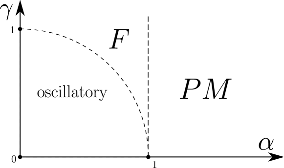
Figure 1: The phase diagram of the considered ferromagnetic XY chain. According to the character of the two-spin correlations, one can distinguish three phases, i.e. a ferromagnetic phase ($F$), which splits into oscillatory and non oscillatory regions, and a paramagnetic phase ($PM$). Parameters $\alpha$ and $\gamma$ are the anisotropy parameter and the magnetic field strength from equation (3).

The most interesting lines on the phase diagram are: i) the vertical line $\alpha=1$, ii) the ’isotropy’ line $\gamma=0$ and iii) the circle $\alpha^{2}+\gamma^{2}=1$. (Here $\alpha$ is magnetic field, and $\gamma$ – anisotropy parameter; proper definitions are given in Sec. 2.) The first line i) has been exhaustively examined; it corresponds to the transition between the paramagnetic and ferromagnetic phases. This transition is in the universality class of two-dimensional classical Ising model [2, 3]. The second line ii) corresponds to the change of the direction of magnetization and is in the universality class of two decoupled Ising models [3].

The third line corresponds to the transition between the ferromagnetic and oscillatory phases. In the literature, some rather vague assertions concerning the nature of this transition have been formulated: ’the thermodynamic functions do not exhibit singularities on this line’ [19], but no derivation has been given. The expression for the ground state energy allows one to deduce that it is infinitely differentiable on this line. In this aspect, the transition between ferromagnetic and oscillatory phases resembles the Kosterlitz-Thouless one, but other aspects of these two transitions turned out to be quite different.

The paper is organized as follows. In the Sec. 2 we define the Hamiltonian and briefly describe its diagonalization, which leads to an explicit expression for the ground-state energy. Its properties (differentiability and asymptotic forms of solution in the neighbourhoods of phase transition lines) are presented in the Sec. 3. The Sec. 4 contains summary of results obtained, comparison with existing results and perspectives for future work.

2 The Hamiltonian and its diagonalization

We consider a spin-$1/2$ chain consisting of $N$ sites. The spin sitting in a given site interacts only with its nearest neighbours. The Hamiltonian of such an interaction is given by $H_{i,j}=J_{x}S^{x}_{i}S^{x}_{j}+J_{y}S^{y}_{i}S^{y}_{j}$, where $i,j$ are the nearest neighbours; we denote it by writing $\langle i,j\rangle$. Moreover, the chain is placed in a transverse magnetic field $h$. Therefore, the Hamiltonian of the whole system is

$$H=\sum_{\langle i,j\rangle}(J_{x}S_{i}^{x}S_{j}^{x}+J_{y}S_{i}^{y}S_{j}^{y})-h\mu\sum_{i=1}^{N}S_{i}^{z}.$$ (1)

The spin operators, $S^{x}$, $S^{y}$ and $S^{z}$ are proportional to the Pauli matrices

$$S^{x}=\frac{1}{2}\begin{pmatrix}0&1\\ 1&0\\ \end{pmatrix},\ \ S^{y}=\frac{1}{2}\begin{pmatrix}0&-i\\ i&0\\ \end{pmatrix},\ \ S^{z}=\frac{1}{2}\begin{pmatrix}1&0\\ 0&-1\\ \end{pmatrix}.$$ (2)

We rewrite expression (1) introducing the anisotropy parameter $\gamma\in[-1,1]$, defined by: $\gamma=\frac{1}{2J}(J_{x}-J_{y})$, where $J=\frac{1}{2}(J_{x}+J_{y})$. Moreover, we denote $h\mu$ as $\alpha$. The Hamiltonian (1), expressed in terms of those parameters is given by

$$H=J\sum_{\langle i,j\rangle}\left[(1+\gamma)S_{i}^{x}S_{j}^{x}+(1-\gamma)S_{i}^{y}S_{j}^{y}\right]-\alpha\sum_{i=1}^{N}S_{i}^{z}.$$ (3)

For $\gamma=0$ Hamiltonian (3) describes fully isotropic interaction, whereas $\gamma=1$ corresponds to the Ising model. We consider the ferromagnetic case, i.e. $J_{x}<0$, $J_{y}<0$.

The Hamiltonian (3) can be rewritten in the language of free fermions. It is done by the so called Jordan-Wigner transformation [1], [20]. For the free-fermion Hamiltonian one can explicitely calculate all eigenvalues and in particular obtain the expression for the ground-state energy.

2.1 Jordan-Wigner transformation and diagonalization of the Hamiltonian

In thus section we give the main points of the Jordan-Wigner transformation. The details can be found for instance in [1], [20]. The first step is to write hamiltonian (3) with $J=-1$ in terms of spin-raising and spin-lowering operators

$$a_{i}^{\dagger}=S_{i}^{x}+iS_{i}^{y},\ \ a_{i}=S_{i}^{x}-iS_{i}^{y}.$$

The hamiltonian then reads

$$H=-\sum_{(i,j)}\frac{1}{2}\left(a_{i}^{\dagger}a_{j}+\gamma a_{i}^{\dagger}a_{j}^{\dagger}+\textrm{h.c.}\right)+\alpha\sum_{j=1}^{N}\left(a_{i}^{\dagger}a_{i}-\frac{1}{2}\right)$$ (4)

The algebraic properties of operators $(a_{i})$ are nonuniform, i.e. the raising and lowering operators from the same site anticommute, while operators from different sites commute. The solution of this problem is the Jordan-Wigner transformation, which introduces the set of $2N$ fermionic operators $\{c_{i}\}$, $\{c^{\dagger}_{i}\}$ given by

$$\begin{cases}c_{i}=\exp\left(\pi i\sum_{j=1}^{i-1}a_{j}^{\dagger}a_{j}\right)a_{i}\\ c_{i}^{\dagger}=a_{i}^{\dagger}\exp\left(-\pi i\sum_{j=1}^{i-1}a_{j}^{\dagger}a_{j}\right)\\ \end{cases}$$ (5)

The operators $c_{i}$ and $c_{i}^{\dagger}$ satisfy purely fermionic commutation rules, i.e.

$$\{c_{i},c_{j}^{\dagger}\}=\delta_{ij},\,\,\{c_{i}^{\dagger},c_{j}^{\dagger}\}=\{c_{i},c_{j}\}=0.$$ (6)

The Hamiltonian of the open chain then reads

$$H=-\frac{1}{2}N\alpha-\sum_{i=1}^{N}\left(\frac{1}{2}\left[c_{i}^{\dagger}c_{i+1}+\gamma c_{i}^{\dagger}c_{i+1}^{\dagger}+\textrm{h.c}\right]-\alpha c_{i}^{\dagger}c_{i}\right)$$ (7)

In calculating the ground state energy in the limit of large $N$, one can impose boundary conditions that are more convenient from the computational point of view, and therefore obtain the c-cyclic chain [1], [20]

$$H=-\frac{1}{2}N\alpha-\sum_{i=1}^{N}\left(\frac{1}{2}\left[c_{i}^{\dagger}c_{i+1}+\gamma c_{i}^{\dagger}c_{i+1}^{\dagger}+\textrm{h.c}\right]-\alpha c_{i}^{\dagger}c_{i}\right),\,\,N+1\equiv 1.$$ (8)

The hamiltonians (7), (8) are quadratic forms in fermion creation and annihilation operators and can be diagonalised, i.e. written in the following form

$$H=E_{g}+\sum_{k=1}^{N}\Lambda_{k}\eta^{\dagger}_{k}\eta_{k},$$ (9)

where $(\eta_{k})$ are some fermionic operators. Assume, we have found the eigenvalues $\Lambda_{k}$ of Hamiltonian (4). In order to find the ground state energy, $E_{g}$, let us calculate the trace of Hamiltonians (4) and (9)

$$\begin{array}[]{c}\mathrm{Tr}(H)=2^{N-1}\sum_{k}\Lambda_{k}+2^{N}E_{g}\\ \hskip 82.51282pt=\alpha\mathrm{Tr}\left\{\sum_{j=1}^{N}\left(a_{i}^{\dagger}a_{i}-\frac{1}{2}\right)\right\}=0.\end{array}$$ (10)

The formula for the ground state energy per spin in the thermodynamic limit does not depend on the boundary conditions, because the difference between the c-cyclic and open chain tend to zero in the thermodynamic limit.

Therefore, in all cases, the ground state energy can be calculated from equation (10), i.e.

$$E_{g}=-\frac{1}{2}\sum_{k}\Lambda_{k}.$$ (11)

The eigenvalues for the cyclic boundary conditions are given by

$$\Lambda_{k}^{2}=\left[\alpha-\cos(k)\right]^{2}+\gamma^{2}\sin^{2}(k),\ k=\frac{2\pi m}{N},\ m=0,1,\dots,N-1.$$ (12)

This expression was derived for the first time by Katsura in [21].

2.2 The formulae for ground state energy

Using fomulae (11) and (12) in the thermodynamic limit, one obtains the ground state energy in a form of the following integral

$$\frac{E_{g}}{N}=-\frac{1}{4\pi}\int_{0}^{2\pi}dt\sqrt{(\alpha-\cos t)^{2}+\gamma^{2}\sin^{2}t}=-\frac{1}{2\pi}\int_{0}^{\pi}dt\sqrt{(\alpha-\cos t)^{2}+\gamma^{2}\sin^{2}t}.$$ (13)

The procedure of calculation of this integral is lengthy and tedious but straightforward. We skip it and present the final result [13] : The ground state energy $\epsilon_{g}$ is given by formulas

$$\epsilon_{g}=\left\{\begin{array}[]{cc}-\frac{\sqrt{1-\alpha^{2}}}{\pi}\Bigg{[}E(k)-K(k)+\frac{1}{1-\alpha^{2}}\Pi\bigg{(}-\frac{\alpha^{2}}{1-\alpha^{2}};k\bigg{)}\Bigg{]}\;,\;\;\;k=\sqrt{\frac{1-\alpha^{2}-\gamma^{2}}{1-\alpha^{2}}},&\mathrm{for}\ \alpha^{2}+\gamma^{2}<1\\ -\frac{1-\alpha^{2}}{\pi\gamma}\Bigg{[}\Pi\big{(}\alpha^{2};k\big{)}-K(k)+\frac{\gamma^{2}}{1-\alpha^{2}}E(k)\Bigg{]}\;,\;\;\;k=\frac{\sqrt{\alpha^{2}+\gamma^{2}-1}}{\gamma},&\mathrm{for}\ \alpha^{2}+\gamma^{2}>1,\ \alpha<1\\ -\frac{\alpha^{2}-1}{\pi\sqrt{\alpha^{2}+\gamma^{2}-1}}\Bigg{[}\Pi\big{(}\frac{1}{\alpha^{2}};k\big{)}-K(k)+\frac{\alpha^{2}+\gamma^{2}-1}{\alpha^{2}-1}E(k)\Bigg{]}\;,\;\;\ k=\frac{\gamma}{\sqrt{\alpha^{2}+\gamma^{2}-1}}&\mathrm{for}\ \alpha^{2}+\gamma^{2}>1,\ \alpha>1.\end{array}\right.$$ (14)

The above results are formulated in terms of complete elliptic integrals [22]:

$$K(k)=\int_{0}^{1}\frac{dz}{\sqrt{(1-z^{2})(1-k^{2}z^{2})}},$$

$$E(k)=\int_{0}^{1}dz\sqrt{\frac{1-k^{2}z^{2}}{1-z^{2}}},$$ (15)

$$\Pi(n;k)=\int_{0}^{1}\frac{dz}{(1-nz^{2})\sqrt{(1-z^{2})(1-k^{2}z^{2})}}.$$

which are called complete elliptic integrals of the first, second and the third kind, respectively. To make the expression more transparent, we plot the function (14) on the Fig. 2.

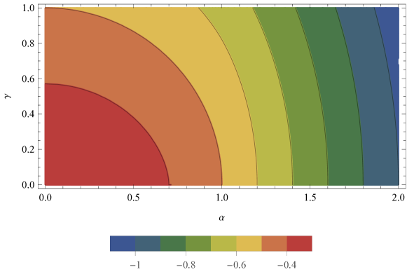
Figure 2: The ground state energy map. The ground state energy is a continuous function with one maximum at $(\alpha,\gamma)=(0,0)$. One characteristic circle-shaped level set can be seen. This is the circle $\alpha^{2}+\gamma^{2}=1$, where $E_{g}=-\frac{1}{2}$.

3 Thermodynamic functions near the phase transition lines

3.1 Magnetization and magnetic susceptibility

The free energy per particle of the system described by a Hamiltonian $H$ is of the form $f=-\frac{1}{N\beta}\ln Z$, where $Z=\mathrm{Tr}e^{-\beta H}$ and $\beta$ is the inverse temperature. When the system is in its ground state, one has to calculate the limit of $f$ as $\beta$ approaches infinity. Therefore

$$f_{g}=\lim_{\beta\rightarrow\infty}\frac{1}{N\beta}\ln Z=\frac{1}{N}\lim_{\beta\rightarrow\infty}\frac{1}{\beta}\mathrm{Tr}e^{-\beta H}=\epsilon_{g}.$$

Then the (transverse) magnetization and the magnetic susceptibility are simply given by

$$\langle M\rangle=-\frac{\partial\epsilon_{g}}{\partial\alpha},\ \ \ \chi=-\frac{\partial^{2}\epsilon_{g}}{\partial\alpha^{2}}.$$ (16)

Differentiating equations (14), one obtains

$$\langle M\rangle=\left\{\begin{array}[]{cc}\frac{1}{\pi\alpha\sqrt{1-\alpha^{2}}}\Big{[}\Pi\Big{(}-\frac{\alpha^{2}}{1-\alpha^{2}};k\Big{)}-(1-\alpha^{2})K(k)\Big{]}\;,\;\;\;k=\sqrt{\frac{1-\alpha^{2}-\gamma^{2}}{1-\alpha^{2}}},&\mathrm{for}\ \alpha^{2}+\gamma^{2}<1\\ \frac{1-\alpha^{2}}{\pi\alpha\gamma}\Big{[}\Pi\big{(}\alpha^{2};k\big{)}-K(k)\Big{]}\;,\;\;\;k=\frac{\sqrt{\alpha^{2}+\gamma^{2}-1}}{\gamma},&\mathrm{for}\ \alpha^{2}+\gamma^{2}>1,\ \alpha<1\\ \frac{\alpha^{2}-1}{\pi\alpha\sqrt{\alpha^{2}+\gamma^{2}-1}}\Pi\big{(}\frac{1}{\alpha^{2}};k\big{)}\;,\;\;\;k=\frac{\gamma}{\sqrt{\alpha^{2}+\gamma^{2}-1}}&\mathrm{for}\ \alpha^{2}+\gamma^{2}>1,\ \alpha>1.\end{array}\right.$$ (17)

and

$$\chi=\left\{\begin{array}[]{cc}\frac{(1-\alpha^{2})E(k)-\gamma^{2}K(k)}{\pi\sqrt{1-\alpha^{2}}(1-\alpha^{2}-\gamma^{2})}\;,\;\;\;k=\sqrt{\frac{1-\alpha^{2}-\gamma^{2}}{1-\alpha^{2}}},&\mathrm{for}\ \alpha^{2}+\gamma^{2}<1\\ \frac{\gamma[K(k)-E(k)]}{\pi(\alpha^{2}+\gamma^{2}-1)}\;,\;\;\;k=\frac{\sqrt{\alpha^{2}+\gamma^{2}-1}}{\gamma},&\mathrm{for}\ \alpha^{2}+\gamma^{2}>1,\ \alpha<1\\ -\frac{K(k)-E(k)}{\pi\sqrt{\alpha^{2}+\gamma^{2}-1}}\;,\;\;\;k=\frac{\gamma}{\sqrt{\alpha^{2}+\gamma^{2}-1}}&\mathrm{for}\ \alpha^{2}+\gamma^{2}>1,\ \alpha>1.\end{array}\right.$$ (18)

The exemplary plots are shown on Figure. 3

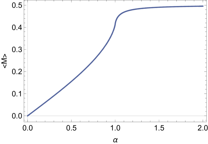
(a)

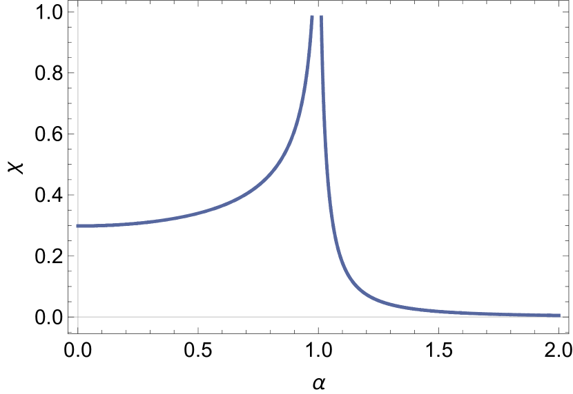
(b)

Figure 3: Magnetisation (a) and magnetic susceptibility (b) for $\gamma=1/3$.

As one can see in figure 3(b), the magnetic susceptibility approaches infinity near $\alpha=1$. Using the series expansions of the complete elliptic integrals near $k=1$ [24], one has that for $|1-\alpha|$ small

$$\chi=\frac{1}{\pi\gamma}\left[\log{\frac{1}{\sqrt{|1-\alpha|}}}+\log\left({2\sqrt{2}\gamma}\right)-1\right]+\frac{8-9\log 2-\gamma^{2}-6\log\gamma}{4\pi\gamma^{3}}|1-\alpha|+\$$

$$+\frac{3}{4\pi\gamma^{3}}|1-\alpha|\log|1-\alpha|+\mathcal{O}(|1-\alpha|^{2}).$$ (19)

Another singularity arises when the second derivative of the energy with respect to $\alpha$ is evaluated around $\gamma=0$ (line ii)). One may expect such a behaviour, because for $\gamma>0$ the x-coupling constant, $J_{x}$, is greater than the y-coupling constant, $J_{y}$ (see eqs. (1) and (3)), while for $\gamma<0$ we have $J_{x}<J_{y}$. This means that while crossing the line $\gamma=0$, the direction of magnetization changes from $x$ to $y$ direction. It turns out that such a transition occurs as an Ising–type singularity, i.e. as a logarithmic divergence of the second derivative. Using the expansions of the elliptic integrals around $1$, $\infty$ or $0$, depending on the value of $k$ for $\gamma$ close to $0$, one can see that this is the case for $\alpha<1$ and $|\gamma|$ small

$$\frac{\partial^{2}\epsilon_{g}}{\partial\gamma^{2}}=\frac{\sqrt{1-\alpha^{2}}}{\pi}\left[2-\frac{\alpha}{\sqrt{1-\alpha^{2}}}\arcsin\alpha+\log\left(\frac{|\gamma|}{4\sqrt{1-\alpha^{2}}}\right)\right]+\frac{1}{4\pi\sqrt{1-\alpha^{2}}}\Big{(}15-21\alpha^{2}+$$

$$-18\alpha\sqrt{1-\alpha^{2}}\arcsin\alpha\Big{)}\gamma^{2}+\frac{9(1-2\alpha^{2})}{8\pi\sqrt{1-\alpha^{2}}}\log\left[\frac{\gamma^{2}}{16(1-\alpha^{2})}\right]\gamma^{2}+\mathcal{O}(|\gamma|^{3}).$$ (20)

For $\alpha>1$ the ground state energy is smooth.

Remark. The transverse susceptibility diverges on both lines $\alpha=1$ and $\gamma=0$ in a logarithmic manner. But the behaviour of the correlation functions is different. The corresponding universality classes for these transitions are called ’Ising model’ and ’two decoupled Ising models’, respectively. They are governed by different correlation functions’ critical exponents [3]. These facts are well known. But using an exact solution, one can obtain the sub-leading exponents as well as amplitudes up to arbitrarily high order. Equations (19) and (20) present the first terms of the expansion.

3.2 Smoothness of the ground state energy on line $\alpha^{2}+\gamma^{2}=1$

In this section we will give the formula for all partial derivatives of function $\epsilon_{g}(\alpha,\gamma)$ (see equation (14)) with respect to parameter $\alpha$ in the limit $\alpha\rightarrow\sqrt{1-\gamma^{2}}^{\pm}$. As shown in section 3.1, the second derivatives of $\epsilon_{g}$ are given by

$$\frac{\partial^{2}\epsilon_{g}}{\partial\alpha^{2}}=\left\{\begin{array}[]{cc}\frac{(1-\alpha^{2})E(k)-\gamma^{2}K(k)}{\pi\sqrt{1-\alpha^{2}}(1-\alpha^{2}-\gamma^{2})}\;,\;\;\;k=\sqrt{\frac{1-\alpha^{2}-\gamma^{2}}{1-\alpha^{2}}},&\mathrm{for}\ \alpha^{2}+\gamma^{2}<1\\ -\frac{\gamma[E(k)-K(k)]}{\pi(\alpha^{2}+\gamma^{2}-1)}\;,\;\;\;k=\frac{\sqrt{\alpha^{2}+\gamma^{2}-1}}{\gamma},&\mathrm{for}\ \alpha^{2}+\gamma^{2}>1,\ \alpha<1.\end{array}\right.$$ (21)

We will next write the above formula in a more compact form, using identities

$$K(k)=\frac{1}{\sqrt{1-k^{2}}}K\left(\frac{ik}{\sqrt{1-k^{2}}}\right),\ \ E(k)=\sqrt{1-k^{2}}E\left(\frac{ik}{\sqrt{1-k^{2}}}\right)$$ (22)

which follow from equations 17.3.29 and 17.3.30 in [23]. For $k=\sqrt{\frac{1-\alpha^{2}-\gamma^{2}}{1-\alpha^{2}}}$, equations (22) read

$$K(k)=\frac{\sqrt{1-\alpha^{2}}}{\gamma}K\left(\tilde{k}\right),\ \ E(k)=\frac{\gamma}{\sqrt{1-\alpha^{2}}}E\left(\tilde{k}\right),$$

where $\tilde{k}=\frac{ik}{\sqrt{1-k^{2}}}=i\frac{1}{\gamma}\sqrt{1-\alpha^{2}-\gamma^{2}}$. Inserting this result to formula (21), one obtains that

$$\frac{\partial^{2}\epsilon_{g}}{\partial\alpha^{2}}=-\frac{\gamma\left[E\left(\tilde{k}\right)-K\left(\tilde{k}\right)\right]}{\pi(\alpha^{2}+\gamma^{2}-1)}=-\frac{1}{\pi\gamma}\frac{\left[E\left(\tilde{k}\right)-K\left(\tilde{k}\right)\right]}{\tilde{k}^{2}},\ \ \alpha<1.$$

We will next use the identity

$$2\frac{\partial E\left(k\right)}{\partial\left(k^{2}\right)}=\frac{\left[E\left(k\right)-K\left(k\right)\right]}{k^{2}},$$

which can be derived using definitions of complete elliptic integrals (equations (15)) simply by subtraction of the integrands on the right hand side and by differentiation under the integral sign on the left hand side. The second derivative of the ground state energy now reads

$$\frac{\partial^{2}\epsilon_{g}}{\partial\alpha^{2}}=-\frac{2}{\pi\gamma}\frac{\partial E\left(k\right)}{\partial\left(k^{2}\right)}\Bigg{|}_{k=\tilde{k}}.$$ (23)

Higher derivatives of the ground state energy can be therefore calculated as derivatives of the composite function $E\left(\tilde{k}^{2}(\alpha,\gamma)\right)$. To this end, we will use the following formula for the $n$th derivative of the composition of two functions [25]

$$\frac{d^{n}}{dx^{n}}f(g(x))=\sum\frac{n!}{k_{1}!k_{2}!\dots k_{n}!}f^{(k)}(g(x))\left(\frac{g^{\prime}(x)}{1!}\right)^{k_{1}}\left(\frac{g^{\prime\prime}(x)}{2!}\right)^{k_{n}}\dots\left(\frac{g^{(n)}(x)}{n!}\right)^{k_{n}},$$ (24)

where the sum runs through all positive integers $k_{1},\dots,k_{n}$ such that $k_{1}+2k_{2}+\dots+nk_{n}=n$ and $k:=k_{1}+k_{2}+\dots+k_{n}$. Note that in the case at hand, the third derivarive of $g(x)=\frac{\partial^{3}\left(\tilde{k}^{2}\right)}{\partial\alpha^{3}}$ vanishes, hence equation (24) simplifies. Namely,

$$\frac{d^{n}}{dx^{n}}f(g(x))=\sum_{k=0}^{\lfloor\frac{n}{2}\rfloor}\frac{n!}{k!(n-2k)!}f^{(n-k)}\left(g(x)\right)\left(g^{\prime}(x)\right)^{n-2k}\left(\frac{1}{2}g^{\prime\prime}(x)\right)^{k}.$$ (25)

Combining the above formula with equation (23), one obtains

$$\lim_{\alpha\rightarrow\sqrt{1-\gamma^{2}}^{\pm}}\frac{\partial^{n+2}\epsilon_{g}}{\partial\alpha^{n+2}}=-\frac{2}{\pi\gamma}\sum_{k=0}^{\lfloor\frac{n}{2}\rfloor}\frac{2^{n-2k}n!}{k!(n-2k)!}\left(\frac{1}{\gamma^{2}}\right)^{n-k}\alpha^{n-2k}\frac{\partial^{n+2}E\left(k\right)}{\partial\left(k^{2}\right)^{n+2}}\Bigg{|}_{k=0},$$ (26)

where the derivatives of function $E(k)$ are known from its series expansion [23]

$$\frac{\partial^{m}E\left(k\right)}{\partial\left(k^{2}\right)^{m}}\Bigg{|}_{k=0}=\frac{\pi}{2}\left[\frac{(2m)!}{2^{2m}(m!)^{2}}\right]^{2}\frac{1}{1-2m}$$ (27)

Both limits of derivatives: left and right ones are equal up to an arbitrary order, so the ground-state energy $\epsilon_{g}$ is infinitely differentiable on the circle $\alpha^{2}+\gamma^{2}=1$.

We have also checked the smoothness of the energy numerically, by plotting the derivatives of the ground state energy of order up to five along some sample curves passing transversally through the circle $\alpha^{2}+\gamma^{2}=1$. The results confirmed our calculations within numerical accuracy.

3.3 The gap energy near the line $\alpha^{2}+\gamma^{2}=1$

Because the character of correlations changes while crossing the line $\alpha^{2}+\gamma^{2}=1$, one could expect that it should result in some kind of singularity. However, as we have shown in previous paragraph, the ground state energy is smooth on the aforementioned circle. Such a behaviour resembles the Kosterlitz-Thouless transition, where certain thermodynamic quantities are smooth. So one can ask whether this transition is present in the considered XY spin chain. Let us shortly review the main properties of the K-T transition, necessary to verify this hypothesis.

The Kosterlitz-Thouless transition occurs in many two-dimensional classical models: Coulomb gas, sine-Gordon, XY and many others [26]. There is no spontaneous symmetry breaking and the free energy, although non-analytic, is infinitely differentiable during this transition. The singular part of the free energy behaves as:

$$f_{sing}\sim\exp\left(-\frac{C}{\sqrt{|T-T_{c}|}}\right)$$

near the critical temperature $T_{c}$ ($C$ is a positive constant). The Kosterlitz-Thouless transition occurs also in ground states of one-dimensional quantum chains under change of certain parameter $\lambda$ (for instance, an anisotropy parameter in the quantum XXZ chain [27]; the $O(2)$ quantum chain [28]; the Ashkin-Teller chain [29], [30]; spin-1 Heisenberg models [31]). In all cases, the ground-state energy is infinitely differentiable, and the energy gap $\Delta E$ over the ground state behaves near the critical value of parameter $\lambda_{c}$ as

$$\Delta E\sim\exp\left(-\frac{C}{\sqrt{|\lambda-\lambda_{c}|}}\right)$$ (28)

($C$ is a positive constant). The physical origin of the Kosterlitz-Thouless sometimes is clear [28], but sometimes is somewhat hidden [27], [30]. So we decided to check whether the K-T transition is present in the XY model. In the following paragraph, we will investigate the aforementioned gap energy i.e. the difference between the energy of the first excited state and the energy of the ground state. First, we will reproduce in an alternative way the well known result regarding the periodic chain. Then, we will show the results of the numerical calculations for an open chain, which reveal that the behaviour of the energy gap is qualitatively the same in both cases. While the energy gap for the cyclic chain is well-studied, the open chain, to our best knowledge, has not yet been investigated. The main reason for this is the lack of the translational symmetry, which makes the exact diagonalization far more difficult. From equation (9), one can easily see that the gap energy is given by the minimal eigenvalue of the Hamiltonian

$$\Delta_{N}(\alpha,\gamma)=\frac{1}{N}\min_{k}\Lambda_{k}.$$ (29)

Let us first reexamine the case of the $c$-cyclic boundary conditions. In order to find the minimal eigenvalue (equation (29)) in the limit of $N\rightarrow\infty$, one has to solve the equation $\frac{d}{dk}\Lambda_{k}=0$, i.e.

$$2\sin k\left(\alpha-\cos k+\gamma^{2}\cos k\right)=0.$$

The gap energy in then given by

$$\lim_{N\rightarrow\infty}N\Delta_{N}(\alpha,\gamma)=\begin{cases}\frac{\gamma}{\sqrt{1-\gamma^{2}}}\sqrt{1-\alpha^{2}-\gamma^{2}}\ \\ |\alpha-1|\ \end{cases}\begin{array}[]{c}\textrm{for }\alpha\leq\sqrt{1-\gamma^{2}},\\ \textrm{for }\alpha>\sqrt{1-\gamma^{2}}\end{array}$$

and it is clear that it does not describe the Kosterlitz-Thouless transition. This result is consistent with the first-order of the expansion for the energy gap, which was derived in [32].

Let us next switch our attention to the open boundary conditions. The hamiltonian of an open chain after the Jordan-Wigner transformation is given by (7). Because of the lack of the translational symmetry, the exact diagonalization of the fermionic Hamiltonian is more difficult, i.e. eigenvalues of one-particle problem are not analytically known for arbitrary $N$. However, one can do the numerical diagonalization. The numerical calculations show that also in the case of an open chain, the gap energy behaves like $1/N$ for sufficiently long chains. The exemplary plots depicting this phenomenon are shown in Figure 5, where the line

$$\Delta_{N}=\frac{a}{N}+\Delta_{\infty}$$ (30)

was fitted.

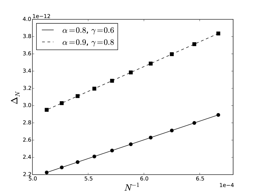
(a) Fitted parameters are: $a=4.33\cdotp 10^{-9},\ \Delta_{\infty}=(-1\pm 2)\cdotp 10^{-27}$ for $\alpha=0.8,\ \gamma=0.6$ and $a=5.75\cdotp 10^{-9},\ \Delta_{\infty}=(-2\pm 3)\cdotp 10^{-27}$ for $\alpha=0.9,\ \gamma=0.8$.

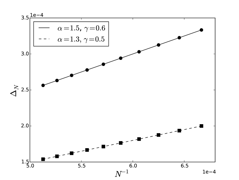
(b) Fitted parameters are: $a=0.5,\ \Delta_{\infty}=(3.43\pm 1.5)10^{-9}$ for $\alpha=1.5,\ \gamma=0.6$ and $a=0.3,\ \Delta_{\infty}=(3.65\pm 1.6)10^{-9}$ for $\alpha=1.3,\ \gamma=0.5$.

Figure 4: The energy gap versus the chain length in (a) weak and (b) strong field.

The fitted values of $\Delta_{\infty}$ are equal to zero within the accuracy of $10^{-27}$ and $10^{-9}$ respectively. The values of parameter $a$ are also fitted very accurately - up to the magnitude of $10^{-24}$ and $10^{-7}$ respectively.

Since $\Delta_{\infty}$ is zero in the whole range of parameters, there is no Kosterlitz-Thouless transition. However, the behaviour of $N\Delta_{N}$ in the limit or large $N$, i.e. parameter $a$ from equation (30), varies significantly on the choice of the boundary conditions. However, in the strong-field region, $\alpha>1$, plots on figure (5) suggest that $a=|\alpha-1|$ regardless on the choice of the boundary conditions.

It turns out that the behaviour of energy gap in the considered XY chain is not compatible with behaviour described by (28). It is so due to the following reasons.

• Consider the ordered phase, i.e. $\alpha>\sqrt{1-\gamma^{2}}$ (and $\alpha<1$). In this ordered phase, the system exhibits the $\mathbb{Z}_{2}$ symmetry [18] (corresponding to plus and minus sign of magnetization), which implies the (asymptotic) degeneracy of two ground states. So, the energy gap is zero in the ordered phase (in the thermodynamic limit).

• Consider the oscillating phase (i.e. $\alpha<\sqrt{1-\gamma^{2}}$) and take the line $\gamma=$const. It turns out that along this line, the gap oscillates. Such a behaviour has been observed in [18]; we illustrate it on Fig. 5. Moreover, for all values of $\alpha$, the gap tends to 0 in the thermodynamic limit.

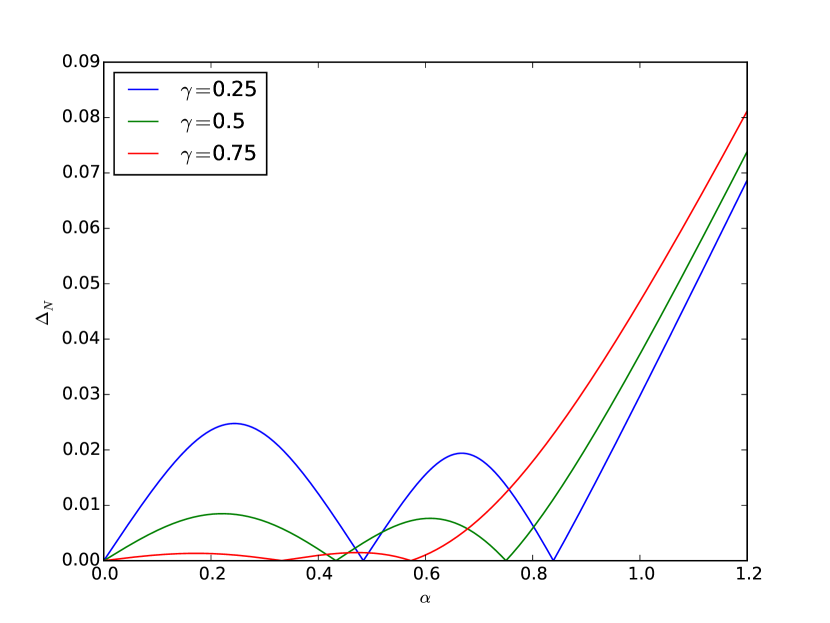
(a) Energy gap for $N=5$.

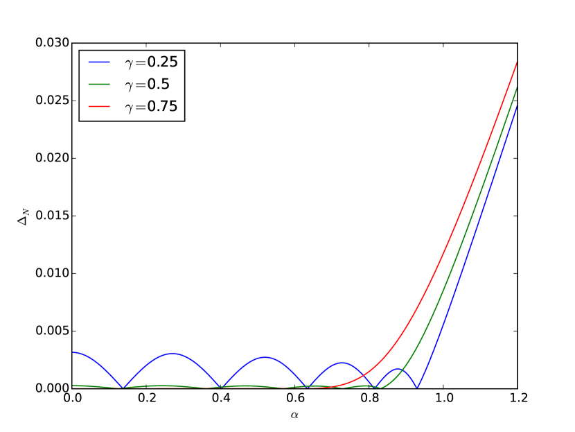
(b) Energy gap for $N=10$.

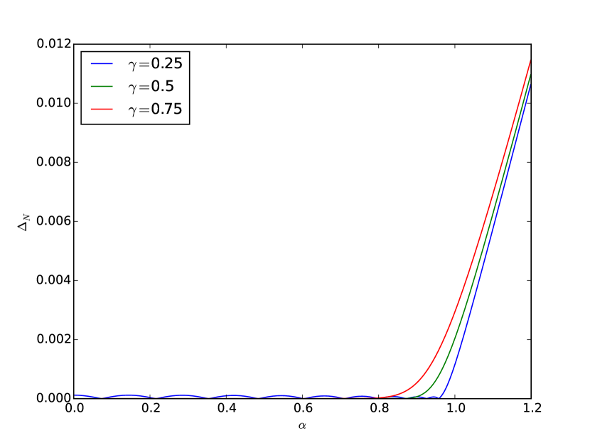
(c) Energy gap for $N=20$.

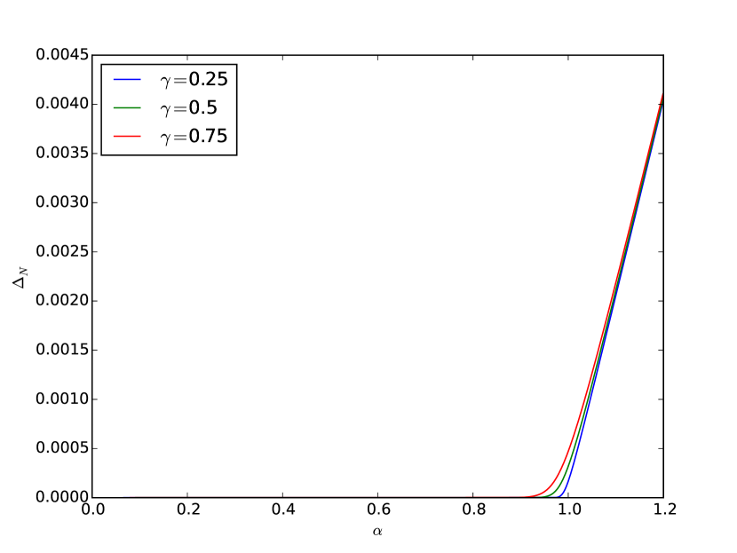
(d) Energy gap for $N=50$.

Figure 5: The energy gap of an open chain for different chain lengths. The oscillatory behaviour for $\alpha<\sqrt{1-\gamma^{2}}$ can be seen. Moreover, with the raise of the chain length the gap tends to zero and the oscillations are faster. For a detailed description, see [18].

We have confirmed numerically that the value of energy gap, extrapolated to $N\to\infty$, is zero. This observation precludes (in a numerical manner) the occurrence of the Kosterlitz-Thouless transition in the XY chain.

The distinguishing feature of K-T transition is the exponential closing of the gap together with the smoothness of ground-state energy at the transition point. In our case, energy gap is asymptotically zero in the neighbourhood of transition point, therefore the gap is not an appropriate object for testing analyticity of the ground-state energy. Intuitively, one could conjecture that the non-analyticity combined with the smoothness of ground-state energy should be somehow related to the structure of energy levels, but we are not able to specify such a relation. More precisely, we don’t know how to formulate asymptotic behaviour of energy levels in the neighbourhood of the circle $\alpha^{2}+\gamma^{2}=1$, and leave this as an open problem. We only conclude that the transition between oscillating and ferromagnetic phases is not of the Kosterlitz-Thouless type.

4 Summary, perspectives for future work

We have analysed the the formula for ground-state energy of the anisotropic XY model in transverse magnetic field. We have examined differentiability properties of the expression. It turned out that the second derivative of energy (i.e. the transverse susceptibility) is logarithmically divergent in the neighbourhood of the lines $\alpha=1$ and $\gamma=0$. This behaviour is characteristic for Ising-type phase transition. This fact has been known earlier (see for instance [3]), but here one can obtain sub-leading exponents and amplitudes up to arbitrary order. We have presented some of first terms of such an expansion.

An interesting open problem (as far as we know) is the question of universality of Ising-type critical behaviour near these lines. The universality principle has been formulated more than 40 years ago, but rigorous proofs are very rare. One of such results is the proof of universality for 2d Ising model due to Spencer [33]. It would be very interesting to adapt the technique used in [33] to quantum XY chain, for lines $\alpha=1$ and $\gamma=0$. On the physical grounds, such universality is expected, but – as far as we know – the rigorous proof is lacking.

We have also established that the energy is differentiable up to arbitrary order on the line $\alpha^{2}+\gamma^{2}=1$. Again, it is interesting to check whether this behaviour is stable (universal) against perturbations of Hamiltonian. Another aspect of the smoothness of energy on the line $\alpha^{2}+\gamma^{2}=1$, it is interesting to confront this result with paper [4], where differentiability property of Renyi entropy has been analysed. The result there is that derivative of Renyi entropy is discontinuous on the line $\alpha^{2}+\gamma^{2}=1$. Apparently, differentiability properties of energy and entropy are different. It seems strange and it would be interesting to take a closer look at this question.

Acknowledgments. We are grateful to Prof. J. Stolze for drawing our attention to paper [13]. Tomasz Maciążek is supported by Polish Ministry of Science and Higher Education “Diamentowy Grant” no. DI2013 016543 and ERC grant QOLAPS.

References

- [1] Lieb, E. H., Schulz, T., and Mattis, D. C.: Ann. Phys. (N. Y. ) 16, 406 (1961).
- [2] Henkel, M.: Conformal Invariance and Critical Phenomena Texts and Monographs in Physics. Springer Verlag, 1999.
- [3] Bunder, J. E. and McKenzie, R. H.: Phys. Rev. B 60, 344 (1999).
- [4] Franchini, F., Its, A. R., and Korepin, V. E.: J. Phys. A: Math. Theor. 41, 025302 (2008); arXiv 0707.2534 [quant-phys]
- [5] Franchini, F., Its, A. R., Jin, B.-Q., and Korepin, V. E.: J. Phys. A: Math. Theor. 40, 8467 (2007)
- [6] Batle, J. and Casas, M.: Phys. Rev. A 82, 062101 (2010)
- [7] Franchini, F., Its, A. R., Korepin, V. E., and Takhtajan, L. A.: Quantum Inf. Process 10, 325 (2011)
- [8] Eisler, V., Karevski, D., Platini, T. and Peschel, I.: J. Stat. Mech. P01023 (2008) arxiv:0711.0289
- [9] Wendenbaum, P. , Platini, T., Karevski, D.: Phys. Rev. A 91, 040303 (2015).
- [10] Pfeuty, P.: Ann. Phys. (N. Y. ) 57, 79 (1970).
- [11] Barouch, E., McCoy, B. M. and Dresden, M.: Phys. Rev. A 2, 1075 (1970)I
- [12] Barouch, E. and McCoy, B. M.: Phys. Rev. A 3, 786 (1971)
- [13] Taylor, J. H. and Müller, G.: Physica 130 A, 1 (1985).
- [14] Vaidya, H. G. and Tracy, C. A.: Physica 92 A, 1 (1978).
- [15] Jimbo, M., Miwa, T., Mori, Y., and Sato, M.: Physica 1 D, 80 (1980).
- [16] Karevski, D.: J. Phys. A33, L313 (2000) arXiv 0009038 [cond-mat]
- [17] Kurmann, J., Thomas, H. and Müller, G.: Physica 112 A, 235 (1982)
- [18] Hoeger, C., von Gehlen, G. and Rittenberg, V.: J. Phys. A 18, 1813 (1985)
- [19] den Nijs, M.: The Domain Wall Theory of Two-Dimensional Commensurate – Incommensurate Phase Transitions. In: Phase Transitions and Critical Phenomena vol. 12, ed. by C. Domb and J. L. Lebowitz, Academic Press, 1988.
- [20] Mattis, D. C.: The Theory of Magnetism II, Springer Series in Solid State Sciences v. 55, Springer Verlag, Berlin, Heidelberg 1985.
- [21] Katsura, S.: Phys. Rev. 127, 1508 (1962).
- [22] Fichtenholz, G. M.: Rachunek różniczkowy i całkowy (Differential and Integral Calculus), vol. 2. Wydawnictwo Naukowe PWN, Warszawa 2013
- [23] Abramowitz, M. and Stegun, I. A. (Eds.). Handbook of Mathematical Functions with Formulas, Graphs, and Mathematical Tables, 9th printing. New York: Dover, 1972
- [24] Whittaker, E. T. and Watson, G. N. A Course in Modern Analysis, 4th ed. Cambridge, England: Cambridge University Press, 1990
- [25] H.-N. Huang, S. A. M. Marcantognini and N. J. Young Chain Rules for Higher Derivatives, 2005 http://www1.maths.leeds.ac.uk/ nicholas/abstracts/FaadiBruno3.pdf
- [26] Kosterlitz J. M. and Thouless, D. J.: J. Phys. C 6, 1181 (1973)
- [27] Šamaj, L.: Acta Phys. Slovaca 60, 155 (2010)
- [28] Allton, C. R. and Hamer, C. J.: J. Phys. A 21, 2417 (1988)
- [29] Kohmoto, M., den Nijs, M., and Kadanoff, L.P.: Phys. Rev. B 24, 5229 (1981)
- [30] Baake, M., von Gehlen, G. and Rittenberg, V.: J. Phys. A 20, L479 and L487 (1987)
- [31] Neirotti, J., P., de Oliveira, M., J., Phys. Rev. B 59, 5 (1998)
- [32] Henkel, M.: J. Phys. A 20, 995 (1987)
- [33] Spencer, T.: Physica 279 A, 250 (2000)