Soft bounds on diffusion produce skewed distributions and Gompertz growth

Abstract

Constraints can affect dramatically the behavior of diffusion processes. Recently, we analyzed a natural and a technological system and reported that they perform diffusion-like discrete steps displaying a peculiar constraint, whereby the increments of the diffusing variable are subject to configuration-dependent bounds. This work explores theoretically some of the revealing landmarks of such phenomenology, termed “soft bound”. At long times, the system reaches a steady state irreversibly (i.e., violating detailed balance), characterized by a skewed “shoulder” in the density distribution, and by a net local probability flux, which has entropic origin. The largest point in the support of the distribution follows a saturating dynamics, expressed by the Gompertz law, in line with empirical observations. Finally, we propose a generic allometric scaling for the origin of soft bounds. These findings shed light on the impact on a system of such “scaling” constraint and on its possible generating mechanisms.

I Introduction

Random processes describe a wide spectrum of phenomena in complex systems Simon:1962 . Diffusion processes, for instance, are used to understand trajectories of one- or multi-dimensional fluctuating observables or order parameters in a great variety of contexts within and outside physics. The validity of such diffusive descriptions – often applicable with impressive precision to real-world systems – is based on the assumption that the probability of future events depends only on the present state of the system Risken:BOOK . Constraints have an influence on such processes, as they limit the phase space that can be reached from a given state.

In one-dimensional diffusion processes, constraints on diffusing quantities are typically embodied by hard bounds, i.e., by strict limits that the diffusing variable cannot overcome, irrespectively of how close or distant to the boundaries the variable already is. The presence of bounds can alter qualitatively the properties of a system. It is well known that absorbing or reflecting boundary conditions affect the basic properties or a random walk, e.g. creating steady-state distributions and affecting first-passage times. Additional more subtle and intriguing phenomena may emerge with hard bounds. For example, a random (diffusional) one-dimensional multiplicative process, in presence of a lower bound, can give rise to power-law distributions for the value of the variable at a given time SornetteCont:1997 ; SolomonLevy:1996 ; AitchisonBrown:BOOK .

However, one can imagine a system where the constraints are not embodied by hard bounds, but follow a different type of behavior. For example discrete diffusion steps may be limited differently depending on the configuration they start from. Recently, we found empirical evidence of precisely this behavior, which we termed soft bound Gherardi:2013PNAS . Note that while a classical physical example of constrained diffusion is a Brownian particle confined in a box, whose motion is continuous in time, in other (often less tangible) examples, such as stock prices MantegnaStanley:BOOK or the population of a city Batty:BOOK , the quantity of interest is naturally measured at discrete time intervals, and its evolution is best described by finite-sized discrete jumps. As we will see, the difference between hard and soft bounds is relevant for time-discrete diffusion processes and we will thus consider this case here.

The scope of this work is to explore some of the basic theoretical consequences of diffusion with soft bounds. It is important to stress that the precise definition of a soft bound — as we formulate it here — is motivated by compelling empirical evidence Gherardi:2013PNAS . The reasons for the emergence of such a behavior constitute a partially unsolved problem (see the Discussion section) and are not the main focus here. Instead, the motivation for the present study is an exploration of its effects. In particular, we present a description of the general features of the stationary state, aided by the analytical solution in a simple case, and we show that a soft upper bound on diffusion causes a slowly saturating dynamics for the maximum. Specifically, we show that detailed balance is broken, and a net local probability current of purely entropic origin is established (which suggests a novel rationalization of the “Cope’s law,” a much debated feature of body mass evolution). Additionally, the steady-state distribution under a soft bound cannot be obtained from a model with a hard bound and an effective drift, and thus has to be regarded as qualitatively distinct from previously known phenomenology. Finally, the dynamics of the maximum follows exactly the Gompertz function, a generalized logistic curve used in diverse contexts and observed empirically. These findings can be used to recognize soft bounds in real-world systems. Finally we argue how a generic allometric scaling mechanism can generate soft bounds.

II Background. Definition of soft bound and empirical evidence

We start by introducing the concept of soft bound through a brief review of the recent empirical evidence suggesting its existence. The first system where the phenomenon of a soft bound emerges from empirical data is the dynamics of software packages, the individual bundled pieces of software that make up an operating system, such as Linux Gherardi:2013PNAS . Packages change their sizes during their lifespan, as a result of development, maintenance, or repackaging. Thus, the scalar variable “size” recapitulates the result of a possibly long and complex series of operations and processes acting on a package. A natural time interval is set by the distance between consecutive package releases: the size $s$ (for instance in bytes) of a given package in a release can be compared to the size $s^{\prime}$ of that same package in the following release, defining a jump $\Delta=s^{\prime}/s$. For Ubuntu Linux packages, these jumps are distributed in a strikingly regular way. While the bulk of their distribution does not depend on time nor on the starting size $s$, its tails are cut-off in a size-dependent way. For jumps towards lower sizes, one expects that the size of a package cannot become smaller than some system-wide minimum $s_{\mathrm{min}}$, i.e. the lower bound is a hard bound. This implies that $\Delta\geq s_{\mathrm{min}}/s$ (the lower bound on the jumps is inversely proportional to the starting size) and this is indeed found in data. However, the same behavior has not been observed for the upper tail of the distribution. In fact, the cut-off for jumps to larger sizes is defined by $\Delta\leq\left(s_{\mathrm{max}}/s\right)^{\gamma}$, with exponent $\gamma\approx 0.5$. This means that the larger a package is, the larger it can become in one step, i.e., the maximum attainable size in one step moves further away for increasingly larger packages (Fig. 1).

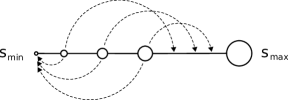
Figure 1: Illustration of the “soft bound” mechanism. In the drawing, the dashed lines stand for the extremal attainable size $s$ in either direction (represented by both circle size and position along the interval) in a single jump, from different initial conditions. Jumps within these limits follow an assigned jump-size distribution. The left-hand side of the interval is conditioned by a conventional hard bound: the minimal size $s_{\mathrm{min}}$ can be reached in a single step starting from any initial size. By contrast, the right-hand part of the interval is limited by a soft bound, as the maximum size attainable in one step depends on the starting size. As a consequence, the absolute maximum $s_{\mathrm{max}}$ cannot be reached in one step from any initial size, but it can only be approached asymptotically.

More formally, in a one-dimensional multiplicative discrete diffusion process limited by a lower hard bound and an upper soft bound, as motivated by the case of Linux package size, the bounds can be expressed by the formula

$$\frac{s_{\mathrm{min}}}{s}\leq\frac{s^{\prime}}{s}\leq\left(\frac{s_{\mathrm{max}}}{s}\right)^{\gamma},\quad\mathrm{with}\;0<\gamma<1.$$ (1)

Regardless of the probability distribution for the jumps $s^{\prime}/s$, such a multiplicative process can be written in an additive form by a logarithmic transformation. By setting $y=\log s$, $x=\log s^{\prime}$, $\Lambda_{\mathrm{min}}=\log s_{\mathrm{min}}$, and $\Lambda_{\mathrm{max}}=\log s_{\mathrm{max}}$, the hard and soft bounds (1) are then expressed by

$$\Lambda_{\mathrm{min}}\leq x\leq y+\gamma\left(\Lambda_{\mathrm{max}}-y\right),$$ (2)

which makes evident the fact that the lower bound $\Lambda_{\mathrm{min}}$ is a hard bound while the upper one depends on the starting point $y$. In the following, unless otherwise specified, we will refer to this additive version of the process.

A second empirical system that is consistent with the diffusion under soft bounds (although data are much sparser) is the evolution of body masses for mammalian species Gherardi:2013PNAS . Here, the time steps are fixed by the speciation events; the “jumps” are realized during cladogenesis between the mass $s$ (in kilograms) of a mother species, and the mass $s^{\prime}$ of the daughter species Clauset2008 ; ClausetRedner:2009 . A notable consequence of the assumption of a soft upper bound in this context is that evolution of mammalian species requires longer time (i.e., more speciation events) to attain large increases in body mass, than it does for large decreases. This macro-evolutionary asymmetry has been observed in fossil data: the tendency to extreme dwarfism, for instance on islands, is more common than the opposite trend EvansJones:2012 .

III Discrete diffusion between a hard and a soft bound

We now define more technically the diffusion process of interest. The formal framework is that of Markov chains. To fix the notation, let $\mathcal{P}_{y\to x}$ denote the transition kernel, i.e., the probability to jump from position $y$ to $x$, and let $\rho_{t}(x)$ be the state of the system, i.e., the density distribution of the diffusing particles at time $t$, e.g. the (logarithmic) package sizes or species masses. This is an inherently discrete process, hence $t$ takes only integer values. State space, instead, is continuous in general. The evolution is then given by

$$\rho_{t+1}(x)=\int_{\mathbb{R}}\mathrm{d}y\,\rho_{t}(y)\,\mathcal{P}_{y\to x}.$$ (3)

We will consider jump probabilities $\mathcal{P}_{y\to x}$ which are the superposition of two components: (i) an underlying transition probability $\pi(x-y)$, which is translationally invariant and does not necessarily have a bounded domain, and (ii) the bounding kernel $\beta(x,y)$, which can be written in terms of a characteristic function as

$$\beta(x,y)=\chi_{[\Lambda_{\mathrm{min}},y+\gamma\left(\Lambda_{\mathrm{max}}-y\right)]}(x).$$ (4)

$\mathcal{P}_{y\to x}$ is then obtained by normalizing the product of the two kernels:

$$\mathcal{P}_{y\to x}=\frac{1}{\mathcal{Z}(y)}\pi(x-y)\beta(x,y),$$ (5)

where $\mathcal{Z}(y)$ is the position-dependent normalization

$$\mathcal{Z}(y)=\int_{\Lambda_{\mathrm{min}}}^{y+\gamma\left(\Lambda_{\mathrm{max}}-y\right)}\!\!\!\pi(x-y)\,\mathrm{d}x.$$ (6)

The dependence of $\mathcal{Z}$ on $y$ makes it difficult in general to find analytic solutions to the evolution, even in the long-time limit.

IV Numerical and analytical characterization of the stationary state

The dynamics defined above has a stationary state, i.e., a distribution $\rho(x)$ that satisfies the following equation:

$$\rho(x)=\int_{\mathbb{R}}\mathrm{d}y\,\rho(y)\,\mathcal{P}_{y\to x}.$$ (7)

The existence of a solution $\rho(x)$ for the above equation will be proven later in this section for a flat underlying transition probability $\pi(x-y)$. Numerical evidence shows that a stationary state is reached also for more general forms of $\pi(x-y)$.

Note that the Markov chain given by the jump distribution $\mathcal{P}_{x\to y}$ in Eq. (5) is irreversible, i.e., the probability of a history $\left(x_{1},\,x_{2},\,\ldots,\,x_{m-1}\right)$ in general differs from that of $\left(x_{m-1},\,x_{m-2},\,\ldots,\,x_{1}\right)$ Kelly:BOOK . This is witnessed by the violation, at the stationary state $\rho(x)$, of the detailed balance condition,

$$\mathcal{P}_{x\to y}\,\rho(x)-\mathcal{P}_{y\to x}\,\rho(y)\equiv 0,$$ (8)

which imposes a vanishing probability flow between any two states $x$ and $y$. Indeed, let $x$ and $y$ be two states lying in the interval $[\Lambda_{min},\,\Lambda_{max})$ and such that $x>y+\gamma\left(\Lambda_{\mathrm{max}}-y\right)$. Since the condition in Eq. (2) is violated, the bounding kernel $\beta(x,y)$ vanishes and then a jump from $y$ to $x$ is suppressed by Eq. (5), i.e. $\mathcal{P}_{y\to x}=0$. However, $x>y$ implies $\mathcal{P}_{x\to y}\not=0$, due to the fact that backward jumps are always allowed by Eq. (2). Consequently, since $\rho(x)\not=0$ (as we will show later in this Section), the detailed balance condition in Eq. (8) can never be satisfied. A more detailed analysis based on entropy production, not relying on the vanishing of $\mathcal{P}$ and only involving two points for which $\beta(x,y)\neq 0$, will be given later in this section.

We explored the properties of the stationary state by analytical and numerical calculations as well as by computer simulations. An analytical approach is unfeasible in general, but it can be carried out in the special case where the transition probability $\pi(x-y)$ is flat between the hard lower bound and the soft upper bound. The salient qualitative features of the steady state realized in this special case do not change if a Gaussian distribution is chosen for $\pi(x-y)$ (see below). To investigate the cases where $\pi(x-y)$ is not flat, one has to take a numerical approach.

Numerical solutions.

We took two different numerical approaches to the solution of the problem: direct numerical integration and Monte Carlo simulations. A numerical approximation of the density distribution $\rho_{t}(x)$ at times $t=0,1,\ldots$ can be obtained by iterative integration, starting from an initial density distribution $\rho_{0}(x)$, by means of Eq. (3). As $\mathcal{P}_{y\to x}$ is different from zero only for $x\in\left[\Lambda_{\mathrm{min}},\,\Lambda_{\mathrm{max}}\right]$, so will be the density distribution $\rho_{t}(x)$, provided that $\rho_{0}(x)$ is supported on the same interval. We defined a spatial discretization of $\rho_{t}(x)$ as follows. Let $\delta x$ be a fixed and small integration step, and define $x_{k}=\Lambda_{min}+k\,\delta x$, with $k=0,1,\ldots,M$, where $M=\lfloor\left(\Lambda_{\mathrm{max}}-\Lambda_{\mathrm{min}}\right)/\delta y\rfloor$ is the largest value of $k$ for which $x_{k}\leq\Lambda_{\mathrm{max}}$. Then the discretized density distribution $\rho_{1}(x_{i})$ at time $t=1$ can be computed from the discretized version of Eq. (3), using the trapezoidal rule. The density distribution at successive time steps is then obtained by iterative application of this procedure.

The Monte Carlo method is based instead on an implementation of the microscopic processes that lead to the continuum description in Eq. (3). In practice, we used a pool of $N$ uncorrelated “particles,” whose positions $y_{i}$ ($i$ is now the particle index) evolve in discrete time steps by following the jump distribution $\mathcal{P}_{y\to x}$. In the following we will choose a delta-shaped initial condition, which translates, at time $t=0$, to all particles being displaced at the same position $x(0)$. At later times, the new position $x_{i}(t+1)=x_{i}(t)+\Delta$ for the $i$-th particle is randomly chosen according to the jump distribution $\mathcal{P}$:

$$\Delta\sim\mathcal{P}_{x_{i}(t)\to x_{i}(t)+\Delta}.$$ (9)

Note that the probability density for the variable $\Delta$ depends explicitly on the position $x_{i}(t)$ of the $i$-th particle at time $t$. If the number of particles $N$ is sufficiently large, the density distribution $\rho_{t}(x)$ can be sampled by a histogram, i.e. a count of the number of particles in the interval $\left[x,x+\delta x\right]$.

Although the two methods are different — numerical integration being deterministic, and Monte Carlo simulation (9) being intrinsically stochastic — they are expected to attain the same results in their “thermodynamic” limits $N\to\infty$ and $\delta y\to 0$. However, since extracting random numbers is computationally more demanding than computing the sum of real numbers, numerical integration results to be faster and more precise than the stochastic method in this situation (however, this is not always the case when different time scales compete, see e.g. Ref. GherardiJourdan ).

Analytical solution for flat transition probability.

Let us consider a flat transition probability $\pi(x-y)=\mathrm{const}$. This gives rise to the simplest possible form of $\mathcal{P}$ with a soft bound. Summing up the definitions given in Eqs. (4)–(6), we obtain the following piecewise continuous function, which for brevity we will term “box distribution”:

$$\mathcal{P}_{y\to x}=\begin{cases}\mathcal{Z}^{-1}\quad&\Lambda_{\mathrm{min}}<x<y+\gamma(\Lambda_{\mathrm{max}}-y)\\ 0&\text{otherwise},\end{cases}$$ (10)

where $\mathcal{Z}={y+\gamma(\Lambda_{\mathrm{max}}-y)-\Lambda_{\mathrm{min}}}$. The stationary distribution $\rho(x)$ satisfies the definition, Eq. (7), which then assumes the form

$$\rho(x)=\int_{y_{\mathrm{inf}}}^{\Lambda_{\mathrm{max}}}\frac{\rho(y)}{y+\gamma(\Lambda_{\mathrm{max}}-y)-\Lambda_{\mathrm{min}}}\,\mathrm{d}y\ ,$$ (11)

where the lower integration bound is

$$y_{\mathrm{inf}}=\max\left\{\Lambda_{\mathrm{min}},\,\frac{x-\gamma\Lambda_{\mathrm{max}}}{1-\gamma}\right\}\ ,$$ (12)

representing the smallest $y$ from where $x$ can be reached in a single jump; the second term in brackets is obtained by inverting the expression of the soft bound, Eq. (2), $x=y+\gamma\left(\Lambda_{\mathrm{max}}-y\right)$. Outside the interval $[\Lambda_{\mathrm{min}},\,\Lambda_{\mathrm{max}}]$, $\rho(x)$ is identically zero. In order to simplify the formulas, and without loss of generality, we can fix $\Lambda_{\mathrm{min}}=0$ and $\Lambda_{\mathrm{max}}=1$ (we will consistently use this convention in the remainder of this section). Hence, $\rho(x)$ becomes

$$\rho(x)=\int_{\max\left\{0,\,\frac{x-\gamma}{1-\gamma}\right\}}^{1}\frac{\rho(y)}{y+\gamma(1-y)}\,\mathrm{d}y,$$ (13)

or equivalently

$$\rho(x)=\rho_{0}-\int_{0}^{\max\left\{0,\,\frac{x-\gamma}{1-\gamma}\right\}}\frac{\rho(y)}{y+\gamma(1-y)}\,\mathrm{d}y\ ,$$ (14)

where $\rho_{0}\equiv\int_{0}^{1}\frac{\rho(y)}{y+\gamma(1-y)}\,\mathrm{d}y$. Note that in this case $\rho(x)$ depends on $x$ only through the boundaries of the definite integral in Eq. (14). Therefore, since the integral depends only on $0<y<\frac{x-\gamma}{1-\gamma}$ for any given $x$, Eq. (14) translates into an iterative procedure for computing the stationary distribution $\rho(x)$, yielding the piecewise analytical solution for adjacent intervals. In fact, for $x<\gamma$ (let us call it interval I), the density distribution is constant and its value is $\rho(x)=\rho_{0}$, because the upper integration bound in Eq. (14) is zero. Now, interval II is defined as the region for which $\rho(x)$ can be calculated from (14) solely in terms of $\rho\left(y\in\mathrm{interval}\;\mathrm{I}\right)$, namely $\gamma<x<1-(1-\gamma)^{2}$. Iterating this procedure, the $n$-th interval is found to be $1-(1-\gamma)^{n-1}<x<1-(1-\gamma)^{n}$, and the analytical form of $\rho(x)$ inside it can be calculated in terms of the $n-1$ solutions already obtained. A few steps are explicitly presented in the Appendix. Figure 2 shows the perfect accordance of the analytical solution with Monte Carlo simulation.

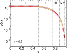
Figure 2: (Color online) The stationary state $\rho(x)$ can be computed analytically by iterative recursion in the case of an underlying flat transition probability. The $n$-th step in the calculation gives the analytical steady state (solid lines) in all intervals up to the $n$-th. (Operatively, one must resort to numerical integration after interval III, see the Appendix.) Circles indicate the results from numerical Monte Carlo simulations (with $10^{6}$ particles). Notice the logarithmic scale on the vertical axis.

It is important to stress here that the behavior of the steady state for a soft bound is qualitatively distinct from a hard bound. As noted before, the stationary state is constant for $0<x<\gamma$ (interval I) and then decreases quickly towards zero in the following intervals. Viewed in logarithmic scale, its shape displays a characteristic shoulder starting at $x=\gamma$, which would be absent if the upper bound were hard (in which case $\gamma=1$). A qualitative comparison of the slope of the shoulder as a function of $\gamma$ can be obtained if one collapses different plots, at different values of $\gamma$, by rescaling $x\mapsto x/\gamma$ and $\rho(x)\mapsto\rho(x)/\rho_{0}$. The result is shown in linear scale in Fig. 3.

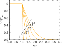
Figure 3: (Color online) The stationary state is flat in the region $(0,\gamma)$. The shoulder shrinks by increasing the parameter $\gamma$. The curves are the steady state distributions (computed by numerical integration) for the case of flat transition probability and soft bounds, plotted as a function of $x/\gamma$, for several values of $\gamma$. The probability density $\rho$ is rescaled by its value in the origin, in order to better compare the different curves. As expected, when the upper bound becomes a hard bound ($\gamma\to 1$), one recovers the usual constant solution for reflective boundary conditions Risken:BOOK .

Entropy production.

As observed above, the diffusion within a soft bound is irreversible; this is signaled by a non-zero entropy production. The entropy production per time step at stationarity Derrida:2007 can be defined for the transition between two states $x$ and $y$ as

$$\Delta S_{x,y}=k\ln\frac{\rho(x)\mathcal{P}_{x\to y}}{\rho(y)\mathcal{P}_{y\to x}},$$ (15)

where $k$ is Boltzmann’s constant. It can be evaluated easily for two states belonging to interval I in Fig. (2), where $\rho(x)/\rho(y)=1$; the difference between the transition probabilities comes from the normalization factor

$$\Delta S_{x,y\in\mathrm{I}}=k\ln\frac{y+\gamma(1-y)}{x+\gamma(1-x)}.$$ (16)

Since this expression is different from zero in general, Eq. (16) shows that the Markov chain is irreversible in a regime where neither $\mathcal{P}_{x\to y}$ nor $\mathcal{P}_{y\to x}$ are vanishing, thus complementing the argument given at the beginning of this Section. For small jumps $y=x+\epsilon$ , the entropy (16) at first order in $\epsilon$ results

$$\Delta S_{x,x+\epsilon}\approx k\epsilon\left(x+\frac{\gamma}{1-\gamma}\right)^{-1},$$ (17)

which is always positive. Consequently, there is a local net imbalance towards larger sizes, which is due solely to the different volumes of configuration space available to different states; in fact, the bulk of the transition probability, close to $x=y$, is symmetric. This tendency is largest for $x$ close to the lower bound, and decreases for larger values of the variable. We point out that a similar trend in the evolution of mammalian body masses (called Cope’s law in this context) has been long studied and debated Cope:1887 ; Gould:1997 ; Clauset2008 , although it is usually ascribed to an asymmetry or a drift in the bulk transition probability. In the soft-bound framework, this feature has entropic origins and emerges naturally.

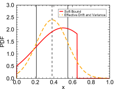
Figure 4: (Color online) Approximation of the soft bound by an effective Gaussian distribution with hard bounds. The Gaussian jump distribution $\mathcal{P^{\prime}}_{y\to x}$ (dashed curve) has mean $\tilde{\mu}$ (vertical dashed line) and variance $\tilde{\sigma}^{2}$ (represented by the vertical solid lines) computed from $\mathcal{P}_{y\to x}$ (solid curve), and is bounded in a size-independent way.

The stationary distribution is not simply the consequence of effective drift and variance.

We now explore in further depth the qualitative differences between a hard and a soft bound. The simple case of a flat $\pi(x-y)$ illustrates the fact that the transition kernel $\mathcal{P}_{y\to x}$ for a given position $y$ is asymmetric in $x$, and the asymmetry depends on $y$. It is then natural to ask whether the same form of the steady state could in principle be obtained by using a symmetric jump distribution $\mathcal{P}^{\prime}_{y\to x}$ with only hard bounds, but adding an effective position-dependent drift and a variance.

To illustrate this point, we consider the situation represented in Fig. 4. Here, the jump distribution $\mathcal{P}_{y\to x}$ (solid curve) is built as in Eq. (5), starting from a Gaussian underlying probability $\pi(x-y)$ with mean zero and variance $\sigma^{2}$. As a consequence of the bounding kernel $\beta(x,y)$, the mean and variance of $\mathcal{P}_{y\to x}$ will be different, and they will have a dependence on $y$ (and of course on the softness parameter $\gamma$). Let us call them $\tilde{\mu}(y,\gamma)$ and $\tilde{\sigma}^{2}(y,\gamma)$ respectively; they are defined as

$$\tilde{\mu}(y,\,\gamma)=\int_{0}^{1}\mathcal{P}_{y\to x}\,x\,\mathrm{d}x$$ (18)

and

$$\tilde{\sigma}^{2}(y,\,\gamma)=\int_{0}^{1}\,\mathcal{P}_{y\to x}\,x^{2}\,\mathrm{d}x-\tilde{\mu}^{2}(y,\gamma).$$ (19)

In Fig. 4, mean and variance are represented respectively by the vertical dashed line and the two vertical solid lines. Note that in general $\tilde{\mu}(y,\,\gamma)\not=0$ and $\tilde{\sigma}^{2}(y,\,\gamma)\not=\sigma^{2}$. The effective distribution $\mathcal{P^{\prime}}_{y\to x}$ (dashed curve in Fig. 4) is constructed as a Gaussian with mean $\tilde{\mu}$, variance $\tilde{\sigma}^{2}$ and lower and upper hard bounds:

$$\mathcal{P}^{\prime}_{y\to x}=\mathcal{Z}^{-1}\chi_{[0,\,1]}(x)\,\exp\left[-\frac{\left(y-\tilde{\mu}\right)^{2}}{2\tilde{\sigma}^{2}}\right].$$ (20)

Note that $\mathcal{P}^{\prime}_{y\to x}\not=\mathcal{P}_{y\to x}$ and, more importantly, $\mathcal{P}^{\prime}_{y\to x}$ does not have any soft bound.

In order to understand if the effects of a soft bound can be recovered by using effective drift and variance, we numerically studied the steady state using both $\mathcal{P}_{y\to x}$ and $\mathcal{P}^{\prime}_{y\to x}$ by varying the variance $\sigma^{2}$ and the soft bound $\gamma$, also in the limit when the soft bound becomes a hard bound. Figure 5 shows that the steady state of the effective jump distribution $\mathcal{P}^{\prime}_{y\to x}$ (green lines) is very different, for most choices of $\sigma$ and $\gamma$, from that obtained using the true soft bound $\mathcal{P}_{y\to x}$ (blue squares). Hence, the effective drift model is in general ineffective. It becomes an acceptable approximation only when $\sigma^{2}$ is small and $\gamma$ is large. In particular, the shoulder characteristic of the soft bound is never well reproduced by the effective process with hard bound and drift.

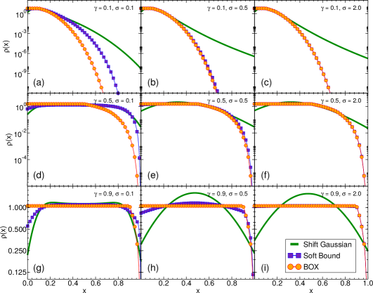
Figure 5: (Color online) The steady state produced by the soft bound (blue squares) is not realized by a discrete Gaussian diffusion with effective drift and variance (green lines). Large values of $\sigma$ give similar results to the analytical solution (orange disks) for a flat jump distribution. Lower values of $\gamma$ give rise to increasingly skewed distributions.

Figure 5 also shows the conditions for which the (analytically computable) steady-state distribution for a soft-bound process with flat transition probability (orange disks in figure) is a good approximation of the soft-bound jump process with a Gaussian transition probability. In brief, for fixed $\gamma<1$, the true steady state approaches (i) the results of the effective drift model when $\sigma\to 0$, and (ii) those for the box distribution when $\sigma\to\infty$. This behavior is easily rationalized by the two facts that (i) the soft bound affects the tail of the jump distribution, and (ii) the Gaussian kernel becomes effectively flat for large variance. The accord for intermediate values of $\sigma$ depends on $\gamma$, and improves for larger values of this parameter (i.e., for harder bounds).

V Dynamics of the maximum and Gompertz law

The nature of the soft bound also affects the relaxation to the steady state. Given an initial distribution $\rho_{0}(x)$, supported in a subinterval of $\left[\Lambda_{\mathrm{min}},\Lambda_{\mathrm{max}}\right)$, one can study the time dependence of the maximum $X_{t}$, i.e., of the largest $x$ on which $\rho_{t}(x)$ is non zero. This may serve as an easily accessible empirical observable, which often turns out to be relevant to characterize the system. For instance, in the evolution of software package sizes, the rightmost point in the support of $\rho_{t}(x)$ represents the evolution of (the logarithm of) the “largest package size” in the operating system. For mammalian body masses, this quantity represents the logarithm of the mass $M_{t}$ of the largest species at a given time $t$, which is the object of much attention in paleobiology, as it can hold information on macro-evolutionary patterns Smith:2010 . For mammals it has been observed, perhaps surprisingly, that this maximum is not dominated by a single taxon nor by a single continent. Different ecological and evolutionary approaches have been applied to the evolution of the maximum mammalian mass. In particular, an unconstrained multiplicative diffusion predicts Trammer:2005 that it grows indefinitely as $X_{t}=\log M_{t}\sim t^{1/2}$. Another model is based on the Gompertz law, a particular logistic function originally proposed as a phenomenological description of mortality in a population Gompertz:1825 (used also in the context of tumor growth Speer:1984 ; AlbanoGiorno:2006 ), and tries to capture in an empirical way the overall effects of constraints, and assumes the following saturating evolution (we use the notation of ref. Smith:2010 ):

$$\log M=\log K-\log\frac{K}{M_{0}}e^{-\alpha t},$$ (21)

where $M_{0}$ is the maximum mass at time 0, $K$ plays the role of a carrying capacity, and $\alpha$ is a characteristic exponent. We show in this section that a Gompertz law for the maximum emerges as a natural consequence of the soft-bound mechanism.

Since we are interested in the evolution of the maximum, the actual shape of $\pi(x-y)$ is not important, as long as its support contains that of $\beta(x,y)$, so that the soft upper bound is the only responsible for the dynamics of $X$. Let $X_{0}=\log M_{0}$ be the maximum at time $0$. Because $\mathcal{P}_{y\to x}$ is bounded by Eq. (2), the maximum $X_{1}$ that can be reach at time $t=1$ will be

$$X_{1}=\Lambda_{\mathrm{max}}+(1-\gamma)(X_{0}-\Lambda_{\mathrm{max}}).$$ (22)

At time $t=2$, the maximum position that can be reached is

$$X_{2} =\Lambda_{\mathrm{max}}+(1-\gamma)(X_{1}-\Lambda_{\mathrm{max}})$$

$$=\Lambda_{\mathrm{max}}+(1-\gamma)^{2}(X_{0}-\Lambda_{\mathrm{max}}).$$

Therefore, the maximum position at time $t$ will be

$$X_{t}=\Lambda_{\mathrm{max}}+(1-\gamma)^{t}(X_{0}-\Lambda_{\mathrm{max}}).$$ (23)

This equation is the logarithmic version of the Gompertz law, i.e., the corresponding law for additive diffusion. Indeed, writing Eq. (23) explicitly for $M_{t}$ yields

$$\log M_{t}=\Lambda_{\mathrm{max}}-\log\frac{M_{0}}{K}e^{\log(1-\gamma)t},$$ (24)

which is the Gompertz law Eq. (21) with $K=\exp(\Lambda_{\mathrm{max}})$ and $\alpha=-\log(1-\gamma)$. We stress that this result is valid independently of the underlying jump distribution $\pi(x-y)$: it is simply the consequence of the functional form of the soft bound, and thus it is very general. Quantitatively, the value $\gamma\approx 0.2$ measured from a compilation of $1109$ ancestor-descendant mass ratios for North American terrestrial mammals Alroy1998 ; Gherardi:2013PNAS yields an estimate $\alpha\approx 0.2$. This is in line with the results ($\alpha\approx 0.1$) obtained from fossil data on the evolution of the largest mammalian mass Smith:2010 .

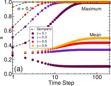
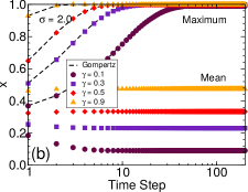
Figure 6: (Color online) The dynamics of the maximum follows precisely the Gompertz function, as is shown analytically in the text. The dynamics of the maximum is independent of the shape of the jump distribution, and only depends on $\gamma$. On the contrary, the dynamics and the stationary value of the mean depend on the details of the distribution; $\sigma=0.1$ in panel (a), $\sigma=2$ in panel (b). Dashed lines are Gompertz functions, symbols are simulations.

Figure 6 compares the analytical solution of Eq. (23) with numerical simulations. The accordance between the two is remarkable. Note that a finite population of $N$ particles does not in general attain exactly the predicted maximum, but finite-size deviations are expected for small $N$. In practice, we expect these errors to likely be negligible for both Ubuntu packages ($N\approx 40\,000$) and mammalian body masses ($N\approx 4000$ in the MOM dataset MOM , used in Ref. Gherardi:2013PNAS ). Also note that, contrary to the maximum, the mean size can either increase or decrease with time in this process, depending on the parameters and on the initial conditions.

VI Discussion and Conclusions

Having shown that the soft bound mechanism is qualitatively distinct from hard bounds, it will be important to determine whether other empirical systems show features that are compatible with the existence of soft bounds. We have analyzed here two main signatures of a soft bound. The first is the formation of a non-trivial shoulder in the steady-state distribution, and the second is the Gompertzian growth of the maximum. These two signatures can be used in practical applications as “smoking guns” for this kind of behavior. Importantly, the soft bound mechanism can be relevant only when the underlying diffusion process has intrinsically discrete nature. We speculate that the soft bound mechanism can occur in situations where the concerted action of many degrees of freedom is proxied by low- or one-dimensional variables (such as “size” or “mass”). In this view, a single jump in size can be seen as the result of a large number of changes in a high-dimensional parameter space, each subject to complex hard bounds (which are more natural to picture), which concur to give rise to the soft bound phenomenon.

Another remarkable feature of a discrete-time diffusion process with soft bounds is the non-reversibility (somewhat analogous to the asymmetry found in the kinetic proofreading BarZiv:2002 ), giving rise to a probability flux of entropic nature. Interestingly, this entropic unbalance, which is naturally present in our model, can provide an alternative (purely entropic) explanation of the Cope’s rule for mammalian evolution.

To conclude, we address a possible generic mechanism that could give rise to soft bounds. Let us consider a complex interacting system with many components or agents, where a scalar order parameter $s$, which we can term “size,” effectively follows a discrete diffusion process. This variable can be for instance the number of lines of a software project, or the mean mass of an animal species, the number of workers in a firm or the number of inhabitants in a city. We suppose that there exists a function, similar to a power in non-equilibrium thermodynamics, estimating the “effort” $E$ that is put into the system for a given span of time. For example the effort can be proxied by the total man-hours spent on the code by programmers, or the food intake of an animal, or the money spent by a firm or city administration. We further assume that a scaling relation

$$E\propto s^{\alpha}$$ (25)

holds between effort and size, where $\alpha$ is an exponent associated to $E$. This assumption can be seen as an instance of allometric scaling, a feature commonly found in complex systems, where some quantity has a power-law dependence on size. It is observed for instance in general ontogenetic growth and the metabolic rates of animals Brody:BOOK ; vonBartalanffy:1957 (albeit with some deviations Kolokotrones:2010 ), transportation networks BanavarMaritan:1999 , and city organization MarsiliZhang:1998 ; Bettencourt:2007 ; LoufBarthelemy:2013 . This relation expresses the principle that the total amount of effort available for the system per unit time can scale sub- or super-linearly with size, with respectively $\alpha<1$ and $\alpha>1$; for the case at hand we suppose $\alpha<1$. Note that Eq. (25), in a thermodynamic interpretation, is different from a Green-Kubo relation where $\alpha=1$ strictly.

We assume the underlying hypothesis that the effort flow is used both for maintaining the system and for increasing its size; the maximum increase, corresponding to exhausting all available effort, thus satisfies

$$s^{\alpha}=c_{\mathrm{m}}s+c_{\mathrm{d}}\left(s^{\prime}-s\right),$$ (26)

where the two constants $c_{\mathrm{m}}$ and $c_{\mathrm{d}}$ are the efforts per unit size needed for maintenance and development respectively. Therefore the maximum multiplicative size change attainable in a given time span is

$$\frac{s^{\prime}}{s}=\frac{s^{\alpha-1}}{c_{\mathrm{d}}}+\left(1-\frac{c_{\mathrm{m}}}{c_{\mathrm{d}}}\right).$$ (27)

If the two cost constants are similar ($c_{\mathrm{d}}\approx c_{\mathrm{m}}$), or when $s^{\prime}/s$ is large, Eq. (27) is just the soft bound Eq. (1), with $\gamma=1-\alpha$ and $s_{\mathrm{max}}=\left(c_{\mathrm{d}}\right)^{-1/\gamma}$. In brief, this argument shows that a scaling hypothesis on the relation between effort-rate and size implies a multiplicative soft bound (similar to the one suggested by both software and mammal mass). We anticipate that the “effort” is not necessarily an abstract quantity, but can be possibly measured in different systems. For example, data is available on the number, extent and frequency of updates of software packages. Thus, the above argument may be (in line of principle) testable, and opens a question for future work.

*

Appendix A

This appendix details some steps of the iterative procedure presented in Sec. IV, for computing the stationary state in the case of a flat jump probability distribution. Starting from Eq. (14), the solution in the interval $0<x<\gamma$ is the constant $\rho(x)=\rho_{0}$. For $\gamma<x<1-(1-\gamma)^{2}$ (interval II) one obtains

$$\rho(x) =\rho_{0}-\int_{0}^{\frac{x-\gamma}{1-\gamma}}\frac{\rho(y)}{y+\gamma(1-y)}\,\mathrm{d}y$$

$$=\rho_{0}\left[1-\int_{0}^{\frac{x-\gamma}{1-\gamma}}\frac{1}{y+\gamma(1-y)}\,\mathrm{d}y\right]$$

$$=\rho_{0}\left[1-\frac{\log(x/\gamma)}{1-\gamma}\right]=\rho_{0}\,\Bigg{[}1-\rho_{1}(x)\Bigg{]}.$$ (28)

The function $\rho_{1}(x)=\log(x/\gamma)/(1-\gamma)$ corresponds to the distribution at time $t=1$ obtained by starting from a constant initial distribution supported on interval I.

Interval III is defined by $1-(1-\gamma)^{2}<x<1-(1-\gamma)^{3}$, and in this region $\rho(x)$ can be calculated as

$$\rho(x) =\rho_{0}\left[1-\int_{0}^{\gamma}\frac{1}{y+\gamma(1-y)}\,\mathrm{d}y-\int_{\gamma}^{\frac{x-\gamma}{1-\gamma}}\frac{1-\rho_{1}(y)}{y+\gamma(1-y)}\,\mathrm{d}y\right]$$

$$=\rho_{0}\left[1-\int_{0}^{\frac{x-\gamma}{1-\gamma}}\frac{1}{y+\gamma(1-y)}\,\mathrm{d}y+\int_{\gamma}^{\frac{x-\gamma}{1-\gamma}}\frac{\rho_{1}(y)}{y+\gamma(1-y)}\,\mathrm{d}y\right]=\rho_{0}\,\Bigg{[}1-\rho_{1}(x)-\rho_{2}(x)\Bigg{]},$$ (29)

where

$$\rho_{2}(x) =-\int_{\gamma}^{\frac{x-\gamma}{1-\gamma}}\frac{\rho_{1}(y)}{y+\gamma(1-y)}\,dy=\frac{\log\left(\frac{x}{\gamma}\right)\log\left(\frac{\gamma(1-\gamma)}{x-\gamma}\right)}{(1-\gamma)^{2}}+\frac{\text{Li}_{2}(\gamma-1)-\text{Li}_{2}(1-\frac{x}{\gamma})}{(1-\gamma)^{2}},$$ (30)

which corresponds to the solution at time $t=2$. Unfortunately, due to the presence of dilogarithm functions $\text{Li}_{2}(\cdot)$ in Eq. (30), the full analytical tractability of $\rho(x)$ is broken for further intervals.

References

- (1) H.A. Simon. The architecture of complexity. Proc. Am. Phil. Soc., 106(6):467–482, 1962.
- (2) H. Risken. The Fokker-Planck equation. Springer, Berlin, 1996.
- (3) D. Sornette and R. Cont. Convergent multiplicative processes repelled from zero: power laws and truncated power laws. J. Phys. I France, 7:431–444, 1997.
- (4) S. Solomon and M. Levy. Spontaneous scaling emergence in generic stochastic systems. Int. J. Mod. Phys. C, 7:745–751, 1996.
- (5) J. Aitchison and J.A.C. Brown. The Lognormal Distribution with special reference to its uses in econometrics. Cambridge University Press, Cambridge, UK, 1957.
- (6) M. Gherardi, S. Mandrà, B. Bassetti, and M. Cosentino Lagomarsino. Evidence for soft bounds in Ubuntu package sizes and mammalian body masses. Proceedings of the National Academy of Sciences U.S.A., 110(52):21054–21058, 2013.
- (7) R.N. Mantegna and H.E. Stanley. An Introduction to Econophysics: Correlations and Complexity in Finance. Cambridge University Press, Cambridge, UK, 1999.
- (8) M. Batty. Cities and Complexity: Understanding Cities Through Cellular Automata, Agent-Based Models, and Fractals. MIT Press, Cambridge, MA, 2005.
- (9) A. Clauset and D.H. Erwin. The evolution and distribution of species body size. Science, 321(5887):399–401, 2008.
- (10) A. Clauset and S. Redner. Evolutionary model of species body mass diversification. Phys. Rev. Lett., 102:038103, 2009.
- (11) Alistair R. Evans, David Jones, Alison G. Boyer, James H. Brown, Daniel P. Costa, S. K. Morgan Ernest, Erich M. G. Fitzgerald, Mikael Fortelius, John L. Gittleman, Marcus J. Hamilton, Larisa E. Harding, Kari Lintulaakso, S. Kathleen Lyons, Jordan G. Okie, Juha J. Saarinen, Richard M. Sibly, Felisa A. Smith, Patrick R. Stephens, Jessica M. Theodor, and Mark D. Uhen. The maximum rate of mammal evolution. Proceedings of the National Academy of Sciences U.S.A., 109(11):4187–4190, 2012.
- (12) F.P. Kelly. Reversibility and Stochastic Networks. Cambridge University Press, 2011.
- (13) M. Gherardi, T. Jourdan, S. Le Bourdiec, and G. Bencteux. Hybrid deterministic/stochastic algorithm for large sets of rate equations. Comput. Phys. Commun., 183:1966–1973, 2012.
- (14) Bernard Derrida. Non-equilibrium steady states: fluctuations and large deviations of the density and of the current. Journal of Statistical Mechanics: Theory and Experiment, 2007(07):P07023, 2007.
- (15) E.D. Cope. The origin of the fittest. Appleton, New York, 1887.
- (16) S.J. Gould. Cope’s rule as psychological artefact. Nature, 385(6613):199–200, 1997.
- (17) F.A. Smith, A.G. Boyer, J.H. Brown, D.P. Costa, T. Dayan, S.K.M. Ernest, A.R. Evans, M. Fortelius, J.L. Gittleman, M.J. Hamilton, E. Larisa Harding, K. Lintulaakso, S.K. Lyons, C. McCain, J.G. Okie, J.J. Saarinen, R.M. Sibly, P.R. Stephens, J. Theodor, and M.D. Uhen. The evolution of maximum body size of terrestrial mammals. Science, 330(6008):1216–1219, 2010.
- (18) J. Trammer. Maximum body size in a radiating clade as a function of time. Evolution, 59(5):941–947, 2005.
- (19) B. Gompertz. On the nature of the function expressive of the law of human mortality, and on a new mode of determining the value of life contingencies. Trans. Royal Soc. London, 115:513–583, 1825.
- (20) J.F. Speer, V.E. Petrosky, M.W. Retsky, and R.H. Wardwell. A stochastic numerical model of breast cancer growth that simulates clinical data. Cancer Res., 44:4124–4130, 1984.
- (21) G. Albano and V. Giorno. A stochastic model in tumor growth. J. Theor. Biol., 242(2):329–336, 2006.
- (22) J. Alroy. Cope’s rule and the dynamics of body mass evolution in north american fossil mammals. Science, 280(5364):731–734, May 1998.
- (23) F.A. Smith, S.K. Lyons, S.K.M. Ernest, K.E. Jones, D.M. Kaufman, T. Dayan, P.A. Marquet, J.H. Brown, and J.P. Haskell. Body mass of late Quaternary mammals. Ecology, 84:3403, 2003.
- (24) R. Bar-Ziv, T. Tlusty, and A. Libchaber. Protein–DNA computation by stochastic assembly cascade. Proceedings of the National Academy of Sciences U.S.A., 99(18):11589–11592, 2002.
- (25) S. Brody. Bioenergetics and growth. Reinhold Pub. Corp., New York, 1945.
- (26) L. von Bartalanffy. Quantitative laws in metabolism and growth. Q. Rev. Biol., 32:217–231, 1957.
- (27) T. Kolokotrones, V. Savage, E.J. Deeds, and W. Fontana. Curvature in metabolic scaling. Nature, 464:753–756, 2010.
- (28) J.R. Banavar, A. Maritan, and A. Rinaldo. Size and form in efficient transportation networks. Nature, 399:130–131, 1999.
- (29) M. Marsili and Y-C. Zhang. Interacting individuals leading to Zipf’s law. Phys. Rev. Lett., 80(12):2741–2744, 1998.
- (30) L.M.A. Bettencourt, J. Lobo, D. Helbing, C. Kühnert, and G.B. West. Growth, innovation, scaling, and the pace of life in cities. Proceedings of the National Academy of Sciences U.S.A., 104(17):7301–7306, 2007.
- (31) R. Louf and M. Barthelemy. Modeling the polycentric transition of cities. Phys. Rev. Lett., 111:198702, 2013.