Estimation for ultra-high dimensional factor model: a pivotal variable detection-based approach

Abstract

For factor model, the involved covariance matrix often has no row sparse structure because the common factors may lead some variables to strongly associate with many others. Under the ultra-high dimensional paradigm, this feature causes existing methods for sparse covariance matrix in the literature not directly applicable. In this paper, for general covariance matrix, a novel approach to detect these variables that is called the pivotal variables is suggested. Then, two-stage estimation procedures are proposed to handle ultra-high dimensionality in factor model. In these procedures, pivotal variable detection is performed as a screening step and then existing approaches are applied to refine the working model. The estimation efficiency can be promoted under weaker assumptions on the model structure. Simulations are conducted to examine the performance of the new method and a real dataset is analysed for illustration.

Keywords: Covariance matrix estimation, factor model, principal component analysis, pivotal variable detection, row sparsity, ultra-high dimension.

1 Introduction

Consider the factor model in the form: for $k=1,\cdots,n$

$$\mathbf{X}_{k}=\mathbf{B}\mathbf{f}_{k}+\mathbf{u}_{k},$$ (1.1)

where $\mathbf{X}_{k}=(X_{k1},\cdots,X_{kp})^{T}\in R^{p}$ are $i.i.d.$ random vectors, $\mathbf{B}\in R^{p\times K}$ is the loading matrix of rank $K$ with $K$ being fixed and small, $\mathbf{f}_{k}\in R^{K\times 1}$ is the factor vector, and $\mathbf{u}_{k}\in R^{p\times 1}$. For identifiability, assume that $\mathrm{cov}(\mathbf{f}_{k},\mathbf{u}_{k})=0$, $\mathrm{cov}(\mathbf{f}_{k})=I_{K}$, $\mathbf{\Sigma}_{u}=\mathrm{cov}(\mathbf{u}_{k})$ is sparse and $\mathbf{B}^{T}\mathbf{B}$ is the $K\times K$ diagonal matrix. Then the covariance of $\mathbf{X}_{k}$ has the form $\mathbf{\Sigma}=\mathbf{B}\mathbf{B}^{T}+\mathbf{\Sigma}_{u}$. During the last decade, many works on the inference of the factor model has been developed, such as, Stock and Watson (1998, 2002), Bai and Ng (2002), Bai (2003), Bai and Li (2012), Fan (2011, 2013), Luo (2011) among others.

When $\mathbf{B}$ is nonsparse, the common factors $\mathbf{f}_{k}$ can affect many or even all $X_{kj},1\leq j\leq p$. Consequently, although $\mathbf{\Sigma}_{u}$ is sparse in this model, $\mathbf{\Sigma}$ is nonsparse in rows. See Luo (2011) and Fan, et al (2013) for example. Thus, existing approaches in the literature may not be feasible to estimate $\mathbf{\Sigma}$ and $\mathbf{B}$. To estimate $\mathbf{\Sigma}$, Luo (2011) suggested a LOw Rank and sparsE Covariance (LOREC) when $p/n\rightarrow 0$ as $n\to\infty$, and Fan, et al (2013) considered the conditional sparsity model and proposed a principal orthogonal complement thresholding method (POET) when $p/n^{2}\rightarrow 0$. Interestingly, because of the special structure of the factor model, in case $\mathbf{\Sigma}$ is sparse such that $n^{1/2}/p\rightarrow 0$ does not hold, the POET estimate cannot be consistent. Both of them cannot handle ultra-high dimension.

On the other hand, when $p$ is very large, it is more often the case that the common factors $\mathbf{f}_{k}$ affect $s_{0}(p)$ components of $\mathbf{X}_{k}$ where $s_{0}(p)$ can be large, but compared with $p$, is still relatively small. The matrix $\mathbf{\Sigma}$ is dense in these rows(columns) and is sparse in the others. Therefore, when we can efficiently detect these rows, the estimation will become much easier in ultra-high dimensional scenarios.

Therefore, we suggest a novel approach to detect the variables that makes the corresponding rows dense. The method is for general covariance matrix estimation. It is worthwhile to mention that for covariance matrix estimation, row sparsity is commonly assumed, see Bickel and Levina (2008), Rothman, Levina and Zhu (2009), Cai and Liu (2011) and Ravikumar et al (2011). However, in some applications, this assumption is restrictive. Variables may have significant differences in their behaviors. Some variables are correlated with many others, while the rest are only related to a few. Consequently, $\mathbf{\Sigma}$ can be dense in some rows and sparse in the others. Consider the personal relation as an example: if each person is treated as a variable and two people are related if they know each other. Then some people, e.g. the public figures, may be related with many others, while most of the others are related with only a few persons. Also in citation analysis with each article or book being viewed as a variable, some articles or books are cited by many others, while most are much less cited. In this paper, we consider another assumption to indicate pivotal variables. That is, there exists an index set $J\subset\{1,\cdots,p\}$ and $J^{c}=\{1,\cdots,p\}\backslash J$, the rows or columns of $\mathbf{\Sigma}$ with indices in $J$ may be nonsparse whereas those with indices in $J^{c}$ are sparse. The detail is given in Section 2. Variables corresponding to the rows that are nonsparse are called the pivotal variables whereas variables corresponding to the sparse rows are called the non-pivotal varibles. we investigate the estimation for the factor model (1.1) when $p$ is ultra-high. In Section 2, we give a method to detect the pivotal variables and a ridge ratio method is suggested to estimate the number of those variables.

In Section 3, the pivotal variable detection (PVD) to the factor model (1.1) is first performed to reduce the estimation difficulty. An algorithm to estimate the covariance matrix $\mathbf{\Sigma}$ is proposed in a generic structure. As POET (Fan, et al 2013) and LOw Rank and sparsE Covariance (LOREC, Luo 2011) are two promising estimation methods for the factor model with relatively high, but not ultra-high dimension $p$, we then in Sections 4 and 5 separately discuss the PVD-based POET and LOREC to show the importance of PVD for us to have more efficient estimation procedures for the factor models when $p$ can be ultra-high. Numerical studies are presented in Section 6.

Introduce some notations first. For matrix $A$ of dimension $p\times p$ and index sets $I_{1}$ and $I_{2}$, write respectively $A_{I_{1}I_{2}}$ as the sub-matrix of $A$ with rows $I_{1}$ and columns $I_{2}$; $A_{I_{1}\cdot},A_{\cdot I_{2}}$ as the sub-matrices consisting of $I_{1}$ rows and $I_{2}$ columns. In particular, the sub-matrix of matrix $\mathbf{\Sigma}_{u}$ is denoted as $\mathbf{\Sigma}_{u,I_{1}I_{2}}$, $\|A\|_{1}$, $\|A\|$ and $\|A\|_{F}$ respectively as the $\ell_{1}$ norm, operator norm, and Frobenius norm of $A$. For any set $I$, $|I|$ denotes the cardinality of $I$. For a square matrix $A$, $\lambda_{\min}(A)$ denotes the minimum eigenvalue of $A$. In addition, $c_{i}$ and $C_{i}$ stand for constants.

2 Pivotal variable detection in high dimensional covariance matrix estimation

2.1 Identification of pivotal variables

Consider the identification of pivotal variables first. Assume the following conditions to distinguish between pivotal and non-pivotal variables. Let $J$ be the index set of pivotal variables with cardinality $|J|=s_{0}(p)$. Let $r_{i}=\sum\limits_{j=1}^{p}\sigma_{ij}^{2}/p$, $1\leq i\leq p$ and $q_{n}=\sqrt{(\log p)^{5}/n}$.

(A1) For some constant $0<\kappa<\infty$, $\kappa^{-1}\leq r_{i}/c_{p}\leq\kappa$ uniformly for $i\in J$, and $\max\limits_{i\notin J}r_{i}=O(\delta_{p})$. Moreover, it holds that $q_{n}=O(c_{p}^{2})$ and $\delta_{p}=o(q_{n})$.

Remark 1.

Condition (A1) means that $q_{n}^{-1}c_{p}^{2}=O(1)$ or $\infty$ and $q_{n}^{-1}\delta_{p}=o(1)$. Since $q_{n}$ will be set to converge to 0, Condition (A1) includes the case of $c_{p}=O(1)$ or $c_{p}\rightarrow\infty$. It also allows $c_{p}\rightarrow 0$ but the rate should not be faster than $\sqrt{q_{n}}$. This condition is to distinguish between those $r_{i}$’s corresponding to pivotal variables and nonpivotal variables through different rates. For the approximate factor model where $\mathbf{\Sigma}=\mathbf{B}\mathbf{B}^{T}+\mathbf{\Sigma}_{u}$, Fan et al (2013) assumed that $p^{-1}\lambda_{\min}(\mathbf{B}^{T}\mathbf{B})>c>0$ for some constant $c$. In practice, this assumption may fail when the common factor $\mathbf{f}_{k}$ only affects part of variables. In Section 3, we show that (A1) can still hold though $p^{-1}\lambda_{\min}(\mathbf{B}^{T}\mathbf{B})>c>0$ fails. In this case, the pivotal variable detection is helpful to get good estimate. Details are referred to Section 3.

Recall that $\mathbf{X}_{k}=(X_{k1},\cdots X_{kp})^{T}\in R^{p},k=1,\cdots,n,$ are $i.i.d.$ observations of $\mathbf{X}$. Let

$$\hat{r}_{i}=\sum\limits_{j=1}^{p}\hat{\sigma}_{ij}^{2}/p,$$

where $\hat{\sigma}_{ij}=n^{-1}\sum\limits_{k=1}^{n}(X_{ki}-\bar{X}_{i})(X_{kj}-\bar{X}_{j})$ and $\bar{X}_{i}=n^{-1}\sum\limits_{k=1}^{n}X_{ki},1\leq i,j\leq p$. Two conditions are assumed below:

(A2)

$\log p=o(n^{1/5})$, $n^{\epsilon_{0}}=o(p)$ for some constant $\epsilon_{0}>0$ and there exists $T_{0}>0$, such that $\sup\limits_{1\leq j\leq p}E\exp(X_{kj}^{2}/t)\leq T_{1}<\infty$ for any $t>T_{0}^{2}$.

(A3)

Let $\theta_{ij}=\mathrm{var}(X_{ki}X_{kj})$. $\max\limits_{1\leq i,j\leq p}\theta_{ij}:=\theta_{0}<\infty$, and $\max\limits_{1\leq i\leq p}\sigma_{ii}<\sigma_{0}<\infty$.

Condition (A2) means that $p$ has order lower than $\exp(n^{1/5})$ but higher than $n^{\epsilon_{0}}$ for some $\epsilon_{0}>0$. In high dimensional setting where $p$ is usually significantly larger than $n$, $n^{\epsilon_{0}}=o(p)$ holds obviously with $\epsilon_{0}=1$. $p<n$ is also allowed when $\epsilon_{0}<1$. When $p$ is fixed, pivotal variable detection makes less sense, we will not discuss this scenario in this paper. The following theorem states the consistency of $\hat{r}_{i}$ of $r_{i}$.

Theorem 1.

Under Conditions (A2) and (A3), we have

$$P\left(\max_{1\leq i\leq p}|\hat{r}_{i}-r_{i}|>C_{0}q_{n}\right)=O(p^{-\delta_{0}})$$

where $M>1+\epsilon_{0}^{-1}+\delta_{0}$ with $\delta_{0}$ being sufficiently small and $C_{0}$ is a constant depending on $M$ and $T_{0}$.

Remark 2.

From the proof in the supplement, we see that $C_{0}>24M^{2}T_{2}^{2}$, where $T_{2}=\max\limits_{1\leq i\neq j\leq p}\|X_{ki}X_{kj}\|_{\psi_{1}}$ being a constant depending on $T_{0}$ and $\|\cdot\|_{\psi_{1}}$ is the $\psi_{1}$ norm (Vershynin, 2011). It can be shown that $T_{2}\leq 2T_{0}^{2}$. Note that the value of $C_{0}$ here is only an upper bound. Since $T_{0}$ is generally unknown, $C_{0}$ is also an unknown constant. Thus, this result is mainly for theoretical justification. However, in Subsection 2.2 below for estimating the number of pivotal variables by a ridge ratio method, we can recommend a value of ridge for practical use without involving this unknown $C_{0}$.

Combining this result with Theorem 1 and Condition (A1), we can shows that the maximum of $\hat{r}_{i}$ with $i\in J^{c}$ is significantly less than minimum of $\hat{r}_{i}$ with $i\in J$. This provides a foundation for the identification of pivotal variables.

Theorem 2.

Under Conditions (A1)-(A3) stated above, we have $\max\limits_{i\in J^{c}}\hat{r}_{i}/\min\limits_{i\in J}\hat{r}_{i}=o_{p}(1)$.

We can see from this proposition that, as $n$ being large, the indices with larger values of $\hat{r}_{i}$ are associated with pivotal variables and those with smaller values of $\hat{r}_{i}$ are associated with non-pivotal variables. Sort $\hat{r}_{i},1\leq i\leq p$ in decreasing order, denoted as $\hat{r}_{(1)}\geq\hat{r}_{(2)}\geq\cdots\geq\hat{r}_{(p)}$. Then the indices associated with $\hat{r}_{(1)},\cdots,\hat{r}_{(s_{0}(p))}$ can be the estimate of $J$, where $s_{0}(p)=|J|$. However, $s_{0}(p)$ is unknown. In the following subsection, we will develop an effective method to estimate $s_{0}(p)$.

2.2 Consistent estimate of the number of pivotal variables

In this section we consider estimating $s_{0}(p)$. A ratio estimate that is based on $\hat{r}_{i}$’s is suggested. It can be used a criterion to estimate $s_{0}(p)$ because of the following observation. Without loss of generality, assume that $J=\{1,\cdots,s_{0}(p)\}$ and that the values of $r_{i},i\in J$ have the decreasing order $r_{1}\geq r_{2}\geq\cdots\geq r_{s_{0}(p)}$. At the population level, $1\geq r_{i+1}/r_{i}>C>0$ for a positive constant $C$ when $1\leq i<s_{0}(p)$ and when $i=s_{0}(p)$, $r_{i+1}/r_{i}\approx 0$. In other words, at the value of $i=s_{0}(p)$, the ratio has a clear dropdown in value. Although when $i>s_{0}(p)$, some ratios may be close to $0/0$, we can add a ridge to make all the ratios well defined. That is, $(r_{i+1}+l)/(r_{i}+l)$ for a very small positive value $l$. Thus, we have, for $i<s_{0}(p)$ and $j>s_{0}(p)$, as long as $l$ is small enough (at the sample level, we let it go to zero at certain rate later),

$$(r_{i+1}+l)/(r_{i}+l)>l/(r_{s_{0}(p)}+l)<1=l/l\approx(r_{j+1}+l)/(r_{j}+l).$$

This means that $s_{0}(p)$ is the minimizer of the ratios over all $i$ with $1\leq i\leq p$. At the sample level, we can replace $r_{i}$ by the corresponding estimates. Recall that $\hat{r}_{(1)}\geq\hat{r}_{(2)}\geq\cdots\geq\hat{r}_{(p)}$ is the decreasing order of $\hat{r}_{i},i=1,\cdots,p$. The sample criterion is

$$R_{i}=\frac{\hat{r}_{(i+1)}+l_{n}}{\hat{r}_{(i)}+l_{n}},\ \ \ \ \ i=1,\cdots,p-1,$$

where $l_{n}\rightarrow 0$ to be specified below. The principle of choosing $l_{n}$ is as follows. First, $l_{n}$ goes to zero such that the minimum of $R_{i}$ can go to zero, and second, the convergence rate of $l_{n}$ to zero should be slower than $r_{s_{0}(p)+1}$ to zero such that $l_{n}$ can be a dominating factor such that $R_{i}$ for $i>s_{0}(p)$ converge to $1$. Then $s_{0}(p)$ and $J$ can respectively be estimated by

$$\hat{s}_{0}(p)=\arg\min\limits_{1\leq i\leq p}R_{i}\quad\mbox{and}\quad\hat{J}=\{i:\hat{r}_{i}\geq\hat{r}_{(\hat{s}_{0}(p))}\}$$ (2.1)

This criterion is in spirit similar to that in Xia, Xu and Zhu (2014). The consistency of $\hat{s}_{0}(p)$ and $\hat{J}$ is stated in the following.

Theorem 3.

Under Conditions (A1)-(A3) in Subsection 2.1, as $l_{n}=O([(\log p)^{5}/n]^{\delta_{1}})$, with $\delta_{1}\in(\frac{1}{4},\frac{1}{2})$, we have $P(\hat{s}_{0}(p)=s_{0}(p))\rightarrow 1$ and $P(\hat{J}=J)\rightarrow 1.$

Theorem 3 imposes a constraint on the order of $l_{n}$. A simple choice can be $l_{n}=[(\log p)^{5}/n]^{3/8}$, which is used in our simulations in Section 6.

3 Application to factor model

3.1 Factor model

Recall the factor model (1.1):

$$\mathbf{X}_{k}=\mathbf{B}\mathbf{f}_{k}+\mathbf{u}_{k},$$

where $\mathbf{u}_{k}\in R^{p\times 1},\mathbf{X}_{k}\in R^{p\times 1}$, $\mathbf{f}_{k}\in R^{K\times 1}$ and $\mathbf{B}$ is a matrix of dimension $p\times K$ and $K$ is an unknown small integer. In addition, assume that rank$(\mathbf{B})=K$, $\mathrm{cov}(\mathbf{f}_{k})=I_{K}$, $\mathrm{cov}(\mathbf{f}_{k},\mathbf{u}_{k})=0$, $\mathbf{B}^{T}\mathbf{B}$ is a diagonal matrix and $\mathbf{\Sigma}_{u}=\mathrm{cov}(\mathbf{u}_{k})$ is a sparse matrix.

Let $\mathbb{B}=\mathbf{B}\mathbf{B}^{T}$. It is easy to see that the covariance matrix of $\mathbf{X}_{k}$ for this model has the form:

$$\mathbf{\Sigma}=\mathbf{B}\mathbf{B}^{T}+\mathbf{\Sigma}_{u}=\mathbb{B}+\mathbf{\Sigma}_{u}.$$ (3.1)

In Fan, et al (2013) and Luo (2011), the rows of the loading matrix $\mathbf{B}$ are nonzero. Thus, the common factors $\mathbf{f}_{k}$ could have impact for many or even all the variables $X_{kj},1\leq j\leq p$. We call (1.1) the nonsparse factor model. A natural way to estimate the loading matrix $\mathbf{B}$ and the factors is through estimating $\mathbf{\Sigma}$. However, it is not easy unless the dimension $p$ is not ultra-high. As we pointed out in the introduction, Luo (2011) requires $p/n\rightarrow 0$ and Fan et al (2013) requires $p/n^{2}\rightarrow 0$ and $n^{1/2}/p\rightarrow 0$.

On the other hand, in factor analysis, it is often the case that many rows of the loading matrix $\mathbf{B}$ have very small or zero values. In other words, the factors can have impact for part of variables and thus although $\mathbf{B}$ is not sparse, the number of variable affected by the factors is not very large compared with the ultra-high dimension $p$. Therefore, a direct way to reduce dimensionality is to first identify those variables who are affected by the factors associated with $\mathbf{B}$. This way offers us a separation between two types of variables who respectively are affected and are not affected by the factors. We apply the pivotal variable detection for this purpose. When the number of pivotal variables $s_{0}(p)$ is much smaller than the original dimension $p$, we can then use either the method in Fan et al (2013) or that in Luo (2011) to estimate $\mathbf{f}_{k},\mathbf{B}$ and $\mathbf{\Sigma}_{u}$ in a dimension-reducing model.

Assume that there exists a subset $J\subseteq\{1,\cdots,p\}$ such that the rows of $\mathbf{B}$ with the index set $J^{c}=\{1,\cdots,p\}\setminus J$ are 0. That is, letting $\mathbf{B}=(\mathbf{b}_{1},\cdots\mathbf{b}_{p})^{T}=(b_{ij})$, then $\mathbf{b}_{j}=0$ for $j\in J^{c}$. Write $\mathbf{B}_{J\bullet}$ as the matrix consisting of the rows with the index set $J$ and $\mathbf{B}_{J^{c}\bullet}$ as the matrix with the rows associated with the index set $J^{c}$. By the definition of $\mathbb{B}$, the factor model can be rewritten as

$$\mathbf{X}_{kJ}=\mathbf{B}_{J\bullet}\mathbf{f}_{k}+\mathbf{u}_{kJ},\ \ \ \ \mathbf{X}_{kJ^{c}}=\mathbf{u}_{kJ^{c}}$$ (3.2)

where $\mathbf{X}_{kJ}$ is the sub-vector of $\mathbf{X}_{k}$ with the index $J$ and $\mathbf{u}_{kJ}$ is defined similarly. Since the factor loading $\mathbf{B}$ is sparse, this model is called the sparse factor model. For model (3.2), it is easy to see that $\mathbf{\Sigma}=\mathbb{B}+\mathbf{\Sigma}$ in which the submatrices $\mathbb{B}_{J^{c}J},\mathbb{B}_{JJ^{c}},\mathbb{B}_{J^{c}J^{c}}$ of $\mathbb{B}$ are zero matrices.

To estimate the corresponding $\mathbf{f}_{k}$, $\mathbf{B}_{J,\bullet}$ and $\mathbf{\Sigma}_{u,JJ}$ that is the submatrix of $\mathbf{\Sigma}_{u}$ with the index set $J$, we first identify the index set $J$. After that, sophisticated methods in the literature can be applied. For the matrix $\mathbf{\Sigma}_{u,J^{c}J^{c}}$ associated with $\mathbf{u}_{kJ^{c}}$, we can estimate it by existing methods. we will discuss it in detail later.

To accommodate the methodology development in this section, we first state the conditions and results in Fan et al (2013) for principal orthogonal complement thresholding (POET). Denote $\lambda_{p,\mathbf{B}}=p^{-1}\lambda_{\min}(\mathbf{B}^{T}\mathbf{B})$. The key condition for POET to work is the pervasive assumption (Assumption 1 in Fan et al (2013)):

$$\lambda_{p,\mathbf{B}}>c>0\ \ \ \mbox{and}\ \ \ p^{-1}\|\mathbf{\Sigma}_{u}\|\rightarrow 0.$$ (3.3)

Under this condition, $\mathbf{\Sigma}$ is a spike matrix, of which the first $K$ largest eigenvalues of $\mathbf{\Sigma}$ increases to infinity at the rate of order $O(p)$. This condition leads the principal component analysis (PCA) to work on constructing a consistent estimate of $\mathrm{span}(\mathbf{B})$. If this condition fails, the POET estimate may be inconsistent.

However, for the factor model (3.2) the pervasive assumption (3.3) may fail to hold. Recall that $\mathbf{B}=(b_{ij})$. Let $b_{\max}=\max\limits_{i,j}|b_{ij}|$ and suppose that $b_{\max}<\infty$. As $|J|/p\rightarrow 0$, then $\lambda_{p,\mathbf{B}}\rightarrow 0$ and (3.3) fails. As a result, POET may not guarantee the consistency of the estimates of $\mathrm{span}(\mathbf{B})$, $\mathbf{\Sigma}_{u}$ and $\mathbf{\Sigma}$. As pointed out by Fan et al (2013), the more variables the common factors can affect, the stronger their signals are and easier they can be detected. In other words, in the case of $|J|$ being small, such as $|J|/p\rightarrow 0$, the signals of the common factors are relatively weak and the detection for them becomes relatively difficult.

Note that the rows and columns of $\mathbf{\Sigma}$ with index $J$ are less sparse in model (3.2). Then our idea is first to estimate the index $J$ by the pivotal variable detection method. Afterwards, we can estimate $\mathbf{\Sigma}$ by separately treating $\mathbf{X}_{kJ}$ and $\mathbf{X}_{kJ^{c}}$. Details are presented in Section 3.2. To detect $J$ correctly, Condition (A1) in Section 2.1 is required. For model (3.2), it is easy to see that $r_{i}=p^{-1}\|\mathbf{B}_{i.}\mathbf{B}^{T}+\mathbf{\Sigma}_{u,i.}\|^{2}$ for $i\in J$ and $r_{i}=p^{-1}\|\mathbf{\Sigma}_{u,i.}\|^{2},i\in J^{c}$. Now, we give sufficient conditions for Condition (A1) by imposing an assumption on $\mathbf{B}$, such that $\|\mathbf{B}_{i.}\mathbf{B}\|^{2}$ dominates $\|\mathbf{\Sigma}_{u,i.}\|^{2}$. Clearly this condition is not the weakest but is easy to understand.

Proposition 1.

For model (3.2), suppose that $q_{n}=O(c_{p}^{2})$ and $\delta_{p}=o(q_{n})$, and

• $\frac{\lambda_{\max}(\mathbf{B}^{T}\mathbf{B})}{\lambda_{\min}(\mathbf{B}^{T}\mathbf{B})}=O(1)$, $\sqrt{p^{-1}c_{p}}/\lambda_{p,\mathbf{B}}=O(1)$,

• $\|\mathbf{\Sigma}_{u}\|=o(\sqrt{p\delta_{p}})$ or $\max_{i\in J^{c}}\|\mathbf{\Sigma}_{u,i.}\|=o(\sqrt{p\delta_{p}})$.

Then Condition (A1) in Subsection 2.1 holds.

Here the assumption $\frac{\lambda_{\max}(\mathbf{B}^{T}\mathbf{B})}{\lambda_{\min}(\mathbf{B}^{T}\mathbf{B})}=O(1)$ is used to guarantee that all $r_{i}$ with $i\in J$ have the same magnitude. Recall that $b_{\max}=\max\limits_{i,j}|b_{ij}|$. As $b_{\max}<\infty$, we can show that $\lambda_{p,\mathbf{B}}>c>0$ in Fan et al (2013) implies $\frac{\lambda_{\max}(\mathbf{B}^{T}\mathbf{B})}{\lambda_{\min}(\mathbf{B}^{T}\mathbf{B})}=O(1)$. Proposition 1 relaxes their assumption such that $\lambda_{p,\mathbf{B}}$ can be $O(1)$ or even tends to 0 at a rate slower than $\sqrt{c_{p}/p}$. In addition, note that for any $0<q\leq 1$, $\|\mathbf{\Sigma}_{u,i.}\|\leq\|\mathbf{\Sigma}_{u,i.}\|_{q}$. If $\mathbf{\Sigma}_{u}$ satisfies the row sparsity with $\max_{1\leq i\leq p}\|\mathbf{\Sigma}_{u,i.}\|_{q}=o(\sqrt{p\delta_{p}})$, condition (2) here holds naturally.

Recall that $\mathbf{\Sigma}_{u}=(\sigma_{u,ij})$, $\mathbf{B}=(b_{ij})$ and $\mathbf{u}_{k}=(u_{k1},\cdots,u_{kp})^{T}\in R^{p},1\leq k\leq n$. We give some conditions below such that $J$ can be consistently estimated.

Theorem 4.

Suppose that (i) Condition (A1) in Subsection 2.1 holds, $\log p=o(n^{1/5})$ and $\mathbf{f}_{k},u_{kj},1\leq j\leq p$ are subgaussian variables; (ii) for some constant $C>0$ such that $b_{\max}$, $\max\limits_{1\leq i,j\leq p}|\sigma_{u,ij}|$, $\|\mathbf{f}_{k}\|_{\psi_{2}}$ and $\max\limits_{1\leq j\leq p}\|u_{kj}\|_{\psi_{2}}$ are bounded above by $C$. Then we have

$$P(\hat{J}=J)\rightarrow 1,$$

where $\hat{J}$ is the estimate of $J$ obtained by the pivotal detection method in Section 2 and the definition of $\|\cdot\|_{\psi_{2}}$ is referred to Vershynin (2011).

3.2 Covariance matrix estimation

We are now in the position to investigate the covariance matrix estimation for model (3.2). Recall that the covariance matrix has the form $\mathbf{\Sigma}=\mathbb{B}+\mathbf{\Sigma}_{u}$ with $\mathbb{B}_{J^{c}J},\mathbb{B}_{JJ^{c}},\mathbb{B}_{J^{c}J^{c}}$ being zero matrices. The blocks of its covariance matrix have the following specific structures:

$$\mathbf{\Sigma}_{JJ^{c}} = \mathrm{cov}(\mathbf{X}_{iJ},\mathbf{X}_{iJ^{c}})=\mathrm{cov}(\mathbf{u}_{iJ},\mathbf{u}_{iJ^{c}})=\mathbf{\Sigma}_{u,JJ^{c}},$$

$$\mathbf{\Sigma}_{J^{c}J^{c}} = \mathrm{cov}(\mathbf{X}_{iJ^{c}})=\mathrm{cov}(\mathbf{u}_{iJ^{c}})=\mathbf{\Sigma}_{u,J^{c}J^{c}},$$ (3.4)

$$\mathbf{\Sigma}_{JJ} = \mathbf{B}_{J\cdot}\mathbf{B}_{J\cdot}^{T}+\mathbf{\Sigma}_{u,JJ}=\mathbb{B}_{JJ}+\mathbf{\Sigma}_{u,JJ},$$

where $\mathbf{\Sigma}_{u,JJ^{c}}$ is the submatrix of $\mathbf{\Sigma}_{u}$ with indices of row $J$ and column $J^{c}$; other quantities are defined similarly. Note that $\mathbf{\Sigma}_{u}$ and $\mathbf{\Sigma}$ have the same block matrices with indexes $(J,J^{c}),(J^{c},J)$ and $(J^{c},J^{c})$ respectively. Since $\mathbf{\Sigma}_{u}$ is sparse, the three block matrices $\mathbf{\Sigma}_{JJ^{c}},\mathbf{\Sigma}_{J^{c}J},\mathbf{\Sigma}_{J^{c}J^{c}}$ of $\mathbf{\Sigma}$ are also sparse. Note that the pivotal variable detection can be applied to identify and consistently estimate the index set $J$, we can then have an estimation strategy to separately estimate these four block matrices that are associated with the index sets $(J,J)$, $(J,J^{c})$, $(J^{c},J)$, and $(J^{c},J^{c})$. First, we can apply the existing thresholding penalty method (e.g. Rothman, Levina and Zhu (2009)) on the corresponding block matrices $\hat{\mathbf{\Sigma}}_{\hat{J}\hat{J}^{c}}$, $\hat{\mathbf{\Sigma}}_{\hat{J}^{c}\hat{J}}$ and $\hat{\mathbf{\Sigma}}_{\hat{J}^{c}\hat{J}^{c}}$ of the sample covariance matrix $\hat{\mathbf{\Sigma}}=n^{-1}\sum_{k=1}^{n}(\mathbf{X}_{k}-\bar{\mathbf{X}})(\mathbf{X}_{k}-\bar{\mathbf{X}})^{T}$ where $\bar{\mathbf{X}}=n^{-1}\sum_{k=1}^{n}\mathbf{X}_{k}$.

Second, we consider how to estimate the block matrix $\mathbf{\Sigma}_{JJ}$ which is the sum of a low rank matrix $\mathbb{B}_{JJ}$ and the sparse matrix $\mathbf{\Sigma}_{u,JJ}$. Note that $\mathbf{\Sigma}_{JJ}$ is the covariance matrix of the submodel $\mathbf{X}_{kJ}=\mathbf{B}_{J\cdot}\mathbf{f}_{k}+\mathbf{u}_{kJ}$, which is a nonsparse factor model. Therefore, existing methods developed for nonsparse factor model can be used to estimate $\mathbf{\Sigma}_{JJ}$ by the data $\mathbf{X}_{k\hat{J}},1\leq k\leq n$. Since the dimension of $\mathbf{X}_{k\hat{J}}$ is $s_{0}(p)$ much smaller than $p$, estimating this sub-model becomes a problem with small or moderate dimension.

The estimation procedure is then summarised to the following four steps.

Step 1. Apply the pivotal variable detection method in Section 2 to consistently estimate the index set $J$. The estimate is defined as $\hat{J}$;

Step 2. Apply an existing method to obtain estimates that are based on the data $\mathbf{X}_{k\hat{J}},k=1,\cdots,n$. In the following two sections, we will give the details about principal orthogonal complement thresholding ( POET, Fan, et al 2013), and low rank and sparse covariance (LOREC, Luo 2011), and the comparisons with these two methods when our method is combined with them.

Step 3. Together with the results in Step 2, use the thresholding method to define an estimate $\hat{\mathbf{\Sigma}}_{u}^{\tau}$ of $\mathbf{\Sigma}_{u}$, see Rothman, Levina and Zhu (2009) and Cai and Liu (2011).

Step 4. $\mathbf{\Sigma}$ is estimated by $\hat{\mathbf{\Sigma}}^{\tau}=\hat{\mathbb{B}}+\hat{\mathbf{\Sigma}}_{u}^{\tau}$, where $\hat{\mathbb{B}}_{\hat{J}^{c}\hat{J}}=0$, $\hat{\mathbb{B}}_{\hat{J}\hat{J}^{c}}=0$ and $\hat{\mathbb{B}}_{\hat{J}^{c}\hat{J}^{c}}=0$.

Now we give some discussions on Step 2. Many methods have been developed to estimate the covariance matrix in the model $\mathbf{X}_{k}=\mathbf{B}\mathbf{f}_{k}+\mathbf{u}_{k}$ without the sparse assumption $\mathbf{B}_{J^{c}\cdot}=0$. As was pointed out before, estimating this model requires strong assumptions, especially on $p$, e.g. $p/n\rightarrow 0$ in Luo (2011). However, our method avoids this difficulty because in Step 2, we consider the factor model (3.2) rather than the full model (1.1), which only involves $s_{0}(p)$ covariates rather than the original $p$ covariates. When $s_{0}(p)$ is small, and then estimation can be much easier and efficient.

In principle, many existing methods can be applied in Step 2. But to make estimation easier and more efficient, the method we use for this purpose highly depends on specific structure of covariance matrix. There are several proposals in the literature such as Chandrasekaran et al. (2010), Agarwal et al. (2011), Fan et al. (2013) and Luo (2011). In this paper, we adopt two methods in Step 2: POET (Fan et al, 2013) and LOREC (Luo, 2011). The pivotal variable detection based POET and LOREC are respectively denoted as PVD-based POET and PVD-based OREC. In Sections 4 and 5, we respectively compare PVD-based POET and POET; and PVD-based OREC and LOREC. Theoretical results in Sections 4 and 5 and numerical results in Section 6 show that our method can improve the performances of POET and LOREC significantly when $s_{0}(p)$ is relatively small compared with $p$.

4 PVD-based LOREC

4.1 A brief review of LOREC

LOw Rank and sparsE Covariance estimator (LOREC, Luo, 2011) deals with the following covariance matrix $\Sigma^{*}$ with the form $\Sigma^{*}=L^{*}+S^{*},$ where $L^{*}$ is a low rank matrix and $S^{*}$ is a sparse matrix. This includes the factor model (3.1) as a special case with $\Sigma^{*}=\mathbf{\Sigma}$, $L^{*}=\mathbf{B}\mathbf{B}^{T}=\mathbb{B}$ and $S^{*}=\mathbf{\Sigma}_{u}$. To get an estimate LOREC solves the following optimization problem:

$$\min_{L,S}\frac{1}{2}\|L+S-\hat{\mathbf{\Sigma}}\|_{F}^{2}+\lambda\|L\|_{*}+\rho\|S\|_{1}$$ (4.1)

where $\hat{\mathbf{\Sigma}}$ is the sample covariance matrix, $\|A\|_{*}$ is the nuclear (trace) norm of matrix $A$, $\lambda$ and $\rho$ are tuning parameters. Let $\hat{\mathbf{\Sigma}}_{L}$ denote the LOREC estimate of $\mathbf{\Sigma}$. This estimation procedure is general, and does not take care of the sparsity of $\mathbb{B}$.

We first give some notations that were introduced in Luo (2011). For any matrix $M\in R^{p\times p}$ with the SVD decomposition $M=UDV^{T}$ with $U\in R^{p\times r},V\in R^{p\times r}$, and a diagonal matrix $D\in R^{r\times r}$. Define the tangent spaces

$$\Omega(M)=\{N\in R^{p\times p}|\mbox{support}(N)\subseteq\mbox{support}(M)\},$$

$$T(M)=\{UY_{1}^{T}+Y_{2}V^{T}|Y_{1},Y_{2}\in R^{p\times r}\}.$$

Define respectively the coherence measures of $\Omega(M)$ and $T(M)$ by

$$\xi(T(M))=\max\limits_{\begin{subarray}{c}N\end{subarray}\in T(M),\|N\|_{2}\leq 1}\|N\|_{\infty},\ \ \ \ \mu(\Omega(M))=\max\limits_{N\in\Omega(M),\|N\|_{\infty}\leq 1}\|N\|_{2}.$$

Typically a matrix $M$ with incoherent row/column spaces would have $\xi(T(M))\leq 1$, and $\xi(T(M))=1$ if the row/column spaces of M contain a standard basis vector. Note that $\xi(T(M))$ can be as small as $O(\sqrt{r/p})$ for a rank-$r$ matrix $M\in R^{p\times p}$. Detailed discussions of the above quantities $\Omega(M),T(M),\xi(T(M))$ and $\mu((M))$ and their implications can be found in Chandrasekaran et al. (2012) and Luo (2011). Let $\mathcal{U}(\epsilon_{0})=\{M\in R^{p\times p}:0<\epsilon_{0}<\lambda_{i}(M)<\epsilon_{0}^{-1}<\infty\},$ where $\lambda_{1}\geq\lambda_{2}\geq\cdots\geq\lambda_{p}$ are the singular value of $M$.

Under certain regularity conditions, Corollary 2 of Luo (2011) shows that $\|\hat{\mathbf{\Sigma}}_{L}-\mathbf{\Sigma}\|=O_{p}(\tilde{v}_{1n})$, where

$$\tilde{v}_{1n}=[\tilde{s}\xi(T(\mathbb{B}))+1]\max\left\{\frac{1}{\xi(T(\mathbb{B}))}\sqrt{\frac{\log p}{n}},\sqrt{\frac{p}{n}}\right\}$$ (4.2)

with $\tilde{s}=\max\limits_{1\leq i\leq p}\sum\limits_{1\leq j\leq p}I(\sigma_{u,ij}\neq 0)$, and $\xi(T(\mathbb{B}))$ can be bounded by $1$ and in some cases, it can be as small as $O(\sqrt{r/p})$. The details can be found in Chandrasekaran et al. (2012). Therefore, $p/n\rightarrow 0$ is a necessary condition to guarantee the consistency of $\hat{\mathbf{\Sigma}}_{L}$. In other words, LOREC can not generate a consistent estimator when $p$ is much larger than $n$ even when $\mathbb{B}$ is sparse in the model (3.1).

4.2 PVD-based LOREC for model (3.2)

In contrast, for the sparse factor model, the pivotal variable detection in Step 1 is to reduce it to model (3.2) to make estimating easier. Let $\hat{J}$ be the estimate obtained by the pivotal variable detection. Then we use LOREC to estimate $\mathbf{\Sigma}_{JJ}=\mathbf{B}_{J}\mathbf{B}_{J}^{T}+\mathbf{\Sigma}_{u,JJ}=\mathbb{B}_{JJ}+\mathbf{\Sigma}_{u,JJ}$. Let $\hat{\mathbf{\Sigma}}_{\hat{J}\hat{J}}=n^{-1}\sum\limits_{k=1}^{n}(\mathbf{X}_{k\hat{J}}-\bar{\mathbf{X}}_{\hat{J}})(\mathbf{X}_{k\hat{J}}-\bar{\mathbf{X}}_{\hat{J}})^{T}$. Replacing $\hat{\mathbf{\Sigma}}$ with $\mathbf{\Sigma}_{\hat{J}\hat{J}}$ in (4.1), we respectively define the estimates $\hat{\mathbb{B}}_{\hat{J}\hat{J}}$ and $\hat{\mathbf{\Sigma}}_{u,\hat{J}\hat{J}}$ of $\mathbb{B}_{JJ}$ and $\mathbf{\Sigma}_{u,JJ}$.

To define the final estimate of $\mathbf{\Sigma}$, Step 4 tells us that what we need to do is to estimate the other elements in $\mathbf{\Sigma}_{u}$. Combining the above estimate of $\mathbf{\Sigma}_{u,JJ}$, we only need to estimate $\sigma_{u,ij}$ for either $i\notin J$ or $j\notin J$. Note that $\sigma_{u,ij}=\sigma_{ij}$ for either $i\notin J$ or $j\notin J$ by (3.2). Thus, we can use $\hat{\sigma}_{ij}=n^{-1}\sum\limits_{k=1}^{n}(X_{ki}-\bar{X}_{i})(X_{kj}-\bar{X}_{j})$ an estimate of $\sigma_{ij}$ for either $i\notin\hat{J}$ or $j\notin\hat{J}$. Since LOREC estimates $\mathbf{\Sigma}_{u}$ by $L_{1}$ penalty function, to make a fair comparison between the PVD-based LOREC and LOREC, we use the same method to estimate $\sigma_{u,ij}$ with $i\notin\hat{J}\ \mbox{or}\ j\notin\hat{J}$. As a result, the soft thresholding penalty function (Rothman, Levina and Zhu, 2009) is applied to $\hat{\sigma}_{ij}$ to define a sparse estimate of $\sigma_{ij}$. Let $\tau_{ij}=C\sqrt{(\log p)/n}$ for either $i\notin\hat{J}$ or $j\notin\hat{J}$. We then obtain an estimate $\hat{\mathbf{\Sigma}}_{u}^{\tau}$ that is related to the thresholding value $\tau_{ij}$. Together with Step 4, we obtain an estimate $\hat{\mathbf{\Sigma}}^{\tau}$ of $\mathbf{\Sigma}$.

To investigate the theoretical property of the estimate, the following condition is similar as that in Theorem 1 of Luo (2011).

(A4)

Let $\Omega_{J}=\Omega(\mathbf{\Sigma}_{u,JJ})$ and $T_{J}=T(\mathbb{B}_{JJ})$. Assume that $\mathbf{\Sigma}_{JJ}\in\mathcal{U}(\epsilon_{0})$, $\mu(\Omega_{J})\xi(T_{J})<1/54$, $s_{0}(p)<n$ and that $\lambda_{n}=\max(\xi(T_{J})^{-1}\sqrt{(\log s_{0}(p))/n},\sqrt{s_{0}(p)/n})$ and $\rho_{n}=\kappa\lambda_{n}$, where $\kappa\in[9\xi(T_{J}),1/(6\mu(\Omega_{J}))]$.

Let $v_{1n}=s\xi(T_{J})\max\left\{\frac{1}{\xi(T_{J})}\sqrt{\frac{\log s_{0}(p)}{n}},\sqrt{\frac{s_{0}(p)}{n}}\right\}$, $v_{2n}=m_{p}\left(n^{-1}\log p\right)^{(1-q)/2}$, where $m_{p}=\max\limits_{1\leq i\leq p}\sum\limits_{1\leq j\leq p}|\sigma_{u,ij}|^{q}$ and $0\leq q<1$, and $s=\max_{i\in J}\sum_{j\in J}I(\sigma_{u,ij}\neq 0)$. Then we have the following conclusion.

Theorem 5.

Under Conditions (A1)–(A3) in Subsection 2.1 and (A4) stated above, for the model (3.2)

$$\|\hat{\mathbf{\Sigma}}_{u}^{\tau}-\mathbf{\Sigma}_{u}\|=O_{p}(v_{1n}+v_{2n}),$$

$$\|\hat{\mathbf{\Sigma}}^{\tau}-\mathbf{\Sigma}\|=O_{p}(v_{1n}+v_{2n}+\lambda_{n}).$$

4.3 A comparison between PVD-based LOREC and LOREC

We now briefly make a comparison with LOREC described in Section 4.1. The comparison consists of two parts. The first part is about the practical implementation. We notice that LOREC is a computationally intensive algorithm. In the simulations in Section 6, we will see this. In the sparse factor model, using PVD to make an initial screening is very helpful in the computational aspect. The second part is about its theoretical properties. As was stated before, the LOREC estimate $\hat{\mathbf{\Sigma}}_{L}$ of $\mathbf{\Sigma}$ has the convergence rate $O_{p}(\tilde{v}_{1n})$, whereas our estimate has the rate of order $v_{1n}+v_{2n}+\lambda_{n}$. Note that

$$v_{1n}+\lambda_{n}=[s\xi(T_{J})+1]\max\left\{\frac{1}{\xi(T_{J})}\sqrt{\frac{\log s_{0}(p)}{n}},\sqrt{\frac{s_{0}(p)}{n}}\right\}.$$

As $\mathbf{B}_{J\cdot}=0$, by the definition of $\xi(T(\cdot))$, it is easy to see that $\xi(T_{J})=\xi(T(\mathbb{B}))\leq 1$ and has a lower bound $O(\sqrt{K/s_{0}(p)})$ (Chandrasekaran, et al, 2012). It is obvious that $s\leq\tilde{s}$. Therefore, it retains that $\lambda_{n}+v_{1n}\leq\tilde{v}_{1n}$. When $m_{p}$ is small, $v_{2n}$ can also be dominated by $v_{1n}+\lambda_{n}$ from the discussion below. These observations suggest that the PVD-based LOREC can generate an estimate with a convergence rate faster than or equal to that of the LOREC estimate.

Further, as was discussed, as $p/n\nrightarrow 0$, the LOREC estimate may be inconsistent. In contrast, when $s_{0}(p)$ is small, the consistency of the PVD-based LOREC estimate can be ensured. This can be observed below. Note that $\xi(T)\leq 1$. We have $v_{1n}\leq s\sqrt{\frac{s_{0}(p)}{n}}=:w_{1n}$ and

$$\lambda_{n} \leq O\left(\max\left\{\sqrt{\frac{s_{0}(p)\log s_{0}(p)}{nK}},\sqrt{\frac{s_{0}(p)}{n}}\right\}\right)=O\left(\sqrt{\frac{s_{0}(p)\log s_{0}(p)}{n}}\right)=:w_{2n},$$

where we have used the fact that $\xi(T(\mathbb{B}))$ has a lower bound $c\sqrt{K/s_{0}(p)}$ for some positive constant $c$. Therefore, as long as $s_{0}(p)$, $s$ and $m_{p}$ are small such that $\max\{w_{1n},w_{2n},v_{2n}\}\rightarrow 0$, where $v_{2n}=m_{p}\left(n^{-1}\log p\right)^{(1-q)/2}$, we have $\|\hat{\mathbf{\Sigma}}^{\tau}-\mathbf{\Sigma}\|\rightarrow_{p}0$. For example, if $\max(s,m_{p})<\infty$, and both $(\log p)/n\rightarrow 0$ and $\sqrt{[s_{0}(p)\log s_{0}(p)]/n}\rightarrow 0$, the PVD-based LOREC estimate is consistent.

5 PVD-based POET

5.1 A brief review of POET

For nonsparse factor model $\mathbf{X}_{k}=\mathbf{B}\mathbf{f}_{k}+\mathbf{u}_{k},1\leq k\leq n$, the covariance matrix has the form

$$\mathbf{\Sigma}=\mathbf{B}\mathbf{B}+\Sigma_{u}=\mathbb{B}+\mathbf{\Sigma}_{u}.$$

Under Assumption (3.3), $\mathbf{\Sigma}$ is a spike matrix with the first $K$ eigenvalue significantly larger than the others. The eigenvalue decomposition of $\hat{\mathbf{\Sigma}}$ is $\hat{\mathbf{\Sigma}}=\sum\limits_{i=1}^{p}\hat{\lambda}_{i}\hat{\eta}_{i}\hat{\eta}_{i}^{T}$, where $\hat{\lambda}_{1}\geq\hat{\lambda}_{2}\cdots\geq\hat{\lambda}_{p}$ are the eigenvalues and $\hat{\eta}_{i}$ are the corresponding eigenvectors. Fan, et al (2013) showed that the estimate $\hat{K}$ of $K$ can be consistent, and span$(\mathbf{B})$ can be consistently estimated by $\mathrm{span}(\hat{\eta}_{1},\cdots,\hat{\eta}_{\hat{K}})$. Moreover, $\mathbf{B}\mathbf{f}_{k}$ and consequently $\mathbf{u}_{k},k=1,\cdots,n$ can also be consistently estimated. As a result, $\hat{\mathbf{\Sigma}}_{u}^{\mathcal{T}}$ obtained by the thresholding method is an estimate of $\mathbf{\Sigma}_{u}$. Then $\mathbf{\Sigma}$ can be consistently estimated by

$$\hat{\mathbf{\Sigma}}^{\mathcal{T}}=\sum\limits_{i=1}^{\hat{K}}\hat{\lambda}_{i}\hat{\eta}_{i}\hat{\eta}_{i}^{T}+\hat{\mathbf{\Sigma}}_{u}^{\mathcal{T}}.$$

In the above procedure, the consistency of $\mathrm{span}(\hat{\eta}_{1},\cdots,\hat{\eta}_{\hat{K}})$ is the prerequisite for the final estimate to be consistent. Without Assumption (3.3), the consistency of $\mathrm{span}(\hat{\eta}_{1},\cdots,\hat{\eta}_{\hat{K}})$ and then of the final estimate $\hat{\mathbf{\Sigma}}^{\mathcal{T}}$ may be questionable. However, as was discussed in Section 3, Assumption (3.3) may fail in model (3.2).

5.2 PVD-based POET for model (3.2)

Again, $J$ is estimated by $\hat{J}$ that is obtained in Step 1. In Step 2, POET is applied to the data $\mathbf{X}_{k\hat{J}},k=1,\cdots,n$ to get an estimate $\hat{\mathbf{u}}_{k\hat{J}}$ of $\mathbf{u}_{kJ}$, for $k=1,\cdots,n$, and $\hat{\mathbf{B}}_{\hat{J}\bullet}$, whose column space is an estimate of span$(\mathbf{B}_{J\bullet})$ where $\mathbf{B}_{J\bullet}$ means the $J\times K$ matrix consisting of the corresponding rows of $\mathbf{B}$ to the index set $J$, and $\hat{\mathbf{B}}_{\hat{J}\bullet}$ is defined similarly. In other words, POET is applied to model (3.2).

Further, recall that $\hat{\sigma}_{ij}=n^{-1}\sum\limits_{k=1}^{n}(X_{ki}-\bar{X}_{i})(X_{kj}-\bar{X}_{j})$ and $\theta_{ij}=\mathrm{var}(X_{ki}X_{kj})$, $1\leq i,j\leq p$. Define an estimate of $\theta_{ij}$ as

$$\hat{\theta}_{ij}=n^{-1}\sum\limits_{k=1}^{n}[X_{ki}X_{kj}-\bar{X}_{i}\bar{X}_{j}-\hat{\sigma}_{ij}]^{2},\ \ 1\leq i,j\leq p.$$

Let $\omega_{n}=\sqrt{1/s_{0}(p)}+\sqrt{\log p/n}$ and define the thresholding values $\tau_{ij}=C\omega_{n}\sqrt{\hat{\theta}_{ij}}$ for $1\leq i,j\leq p$. Then Steps 3 and 4 of the algorithm can be reformulated as follows.

Step 3’. Define the vectors $\tilde{\mathbf{u}}_{k},k=1,\cdots,n$, such that $\tilde{\mathbf{u}}_{k\hat{J}}=\hat{\mathbf{u}}_{k\hat{J}}$ and $\tilde{\mathbf{u}}_{k\hat{J}^{c}}=\mathbf{X}_{k\hat{J}^{c}}$. Apply the adaptive thresholding estimate to data $\tilde{\mathbf{u}}_{k},k=1,\cdots,n$ to obtain the estimate $\hat{\mathbf{\Sigma}}_{u}^{\tau}$ of $\mathbf{\Sigma}_{u}$, using the thresholding value $\tau_{ij}$. The reader can refer to Fan, et al (2013) for details.

Step 4’. $\mathbf{\Sigma}$ is estimated by $\hat{\mathbf{\Sigma}}^{\tau}=\hat{\mathbf{B}}\hat{\mathbf{B}}^{T}+\hat{\mathbf{\Sigma}}_{u}^{\tau}$, where $\hat{\mathbf{B}}_{\hat{J}^{c}\bullet}=0$.

Since POET uses the adaptive thresholding method suggested by Cai and Liu (2011) to estimate $\mathbf{\Sigma}_{u}$, in Step 3’, we also use this method such that POET and PVD-based POET can be compared fairly. Again, as POET is used, we assume the following condition in which Part (iia-c) are the adapted versions of Assumptions 2 and 4 in Fan, et al (2013) in our setting.

(A5)

Assume that

(i) $s_{0}(p)^{-1}\lambda_{\min}(\mathbf{B}_{J\bullet}^{T}\mathbf{B}_{J\bullet})$ is bounded away from both 0 and $\infty$ as $p\rightarrow\infty$.

(iia) There are constants $c_{1}$ and $c_{2}>0$ such that $\lambda_{\min}(\mathbf{\Sigma}_{u})>c_{1},\|\mathbf{\Sigma}_{u}\|_{1}<c_{2}$ and $\min\limits_{i\leq p,j\leq p}\mathrm{var}(u_{it}u_{jt})>c_{1}.$

(iib) There are $b_{1}$ and $b_{2}>0$ such that for any $a>0,i\leq p$ and $j\leq K$,

$$P(|u_{it}|>a)\leq\exp(-(a/b_{1})^{2}),\ \ \ \ P(|f_{jt}|>a)\leq\exp(-(a/b_{2})^{2}).$$

(iic) There exists an $M>0$ such that for all $i\in J$ and $t=1,2$ all of the quantities $\|\mathbf{b}_{i}\|_{\max}$, $E[s_{0}(p)^{-1/2}\{\mathbf{u}_{1J}^{T}\mathbf{u}_{tJ}-E(\mathbf{u}_{1J}^{T}\mathbf{u}_{tJ})\}]^{4}$, and $E\|s_{0}(p)^{-1/2}\sum\limits_{i\in J}\mathbf{b}_{i}u_{i1}\|^{4}$ are smaller than $M$.

Recall that $\mathbf{B}_{J^{c}\bullet}=0$ in our setting. It is easy to see that part (i) of Condition (A5) is weaker than the pervasive assumption (3.3) (Assumption 1 in Fan et al (2013)), which requires that $p^{-1}\lambda_{\min}(\mathbf{B}^{T}\mathbf{B})>c>0$. Part (ii) are parallel to Assumptions 2 and 4 in Fan et al (2013). Condition (A5) ensures that when $(s_{0}(p))^{-1}\mathbf{B}_{J\bullet}^{T}\mathbf{B}_{J\bullet}>c>0$, but $p^{-1}\mathbf{B}^{T}\mathbf{B}\rightarrow 0$, our estimate can still be consistent. Let $\gamma=\frac{4}{13}$ and $m_{p}=\max\limits_{1\leq i\leq p}\sum\limits_{1\leq j\leq p}|\sigma_{u,ij}|^{q},$ for some $q\in[0,1]$, controlling the sparsity of $\mathbf{\Sigma}_{u}$.

Theorem 6.

Suppose that $\log p=o(n^{\gamma/6}),n=o(s_{0}(p)^{2})$ and Conditions (A1)-(A3) in Subsection 2.1 and Condition (A5) stated above hold. Then

$$\|\hat{\mathbf{\Sigma}}_{u}^{\tau}-\mathbf{\Sigma}_{u}\| = O_{p}(w_{n}^{1-q}m_{p}),$$

$$\|\hat{\mathbf{\Sigma}}^{\tau}-\mathbf{\Sigma}\|_{\mathbf{\Sigma}} = O_{p}\left(w_{n}^{1-q}m_{p}+p^{-1/2}s_{0}(p)\omega_{n}^{2}\right),$$

where $\|A\|_{\mathbf{\Sigma}}=p^{-1/2}\|\mathbf{\Sigma}^{-1/2}A\mathbf{\Sigma}^{-1/2}\|_{F}$ defined in Fan et al (2013).

5.3 A comparison between PVD-based POET and POET

Let $\hat{\mathbf{\Sigma}}_{P}$ denote the POET estimate of $\hat{\mathbf{\Sigma}}$. Theorem 3 of Fan, et al (2013) provides that

$$\|\hat{\mathbf{\Sigma}}_{P}-\mathbf{\Sigma}\|_{\mathbf{\Sigma}}=O_{p}\left(\tilde{w}_{n}^{1-q}m_{p}+n^{-1}p^{1/2}\log p\right),$$ (5.1)

where $\tilde{\omega}_{n}=\sqrt{(\log p)/n}+\sqrt{1/p}$. First, as $0<d_{1}<s_{0}(p)/p\leq d_{2}\leq 1$ for some constant $d_{1}$ and $d_{2}$, $\omega_{n}^{2}s_{0}(p)p^{-1/2}=O(p^{1/2}n^{-1}\log p)$ by Theorem 6 and PVD-based POET obtains exactly the same convergence rate for $\|\hat{\mathbf{\Sigma}}^{\tau}-\mathbf{\Sigma}\|_{\mathbf{\Sigma}}$ as POET. Second, when $s_{0}(p)/p\rightarrow 0$, the signals of common factor are weak. PVD-based POET can have better convergence rate than POET and latter may not be consistent. It is clear from (5.1) that, as $p$ is large such as $p^{1/2}n^{-1}\rightarrow\infty$, the relative error $\|\hat{\mathbf{\Sigma}}_{P}-\mathbf{\Sigma}\|_{\mathbf{\Sigma}}$ will not converge to zero, regardless of the rate of $m_{p}$. This inevitably requires a strong restriction on the rate of $p$. However, for PVD-based POET method, as long as $s_{0}(p)=o(p^{1/2}n/\log p)$ and $n=o(s_{0}(p)^{2})$ (the assumption required by Theorem 6), we have $\omega_{n}^{2}s_{0}(p)p^{-1/2}=o(1)$. In this case, the relative error $\|\hat{\mathbf{\Sigma}}^{\tau}-\mathbf{\Sigma}\|_{\mathbf{\Sigma}}=O_{p}(\omega_{n}^{1-q}m_{p})$ depends on the sparsity of $\mathbf{\Sigma}_{u}$. The consistency can hold when $m_{p}$ is small. For example, if $m_{p}=o(n^{(1-q)/4})$, then by the assumption that $n=o(s_{0}(p)^{2})$, $\log p=o(n^{1/5})$ and the definition of $\omega_{n}$, it is easy to verify that $\omega_{n}^{1-q}m_{p}\rightarrow 0$. The simulation results in Section 6 confirm the conclusions here.

6 Simulations and real data analysis

Let $\mathbf{\Sigma}=(\sigma_{ij})$ and $\mathbf{X}_{1},\cdots,\mathbf{X}_{n}$ are i.i.d. observations from $N_{p}(0,\mathbf{\Sigma})$. For simplicity, we take $J=\{1,\cdots,p_{1}\}$ and $J^{c}=\{p_{1}+1,\cdots,p\}$.

6.1 Pivotal variable detection

In this simualtion, the sample size is $n=100$ and the dimension is $p=1000$. The experiments are repeated $T$ times to get $\hat{J}_{t},t=1,\cdots,T$. Let Mean and SD respectively stand for the mean and standard deviation of the cardinality $|\hat{J}_{t}|$ of the set $\hat{J}_{t}$ with $t=1,\cdots,T$; let EQ denote the frequency of $\hat{J}_{t}$ being exactly equal to $J$; FP and FN respectively denote the false positive rate and false negative rate:

$$EQ=\frac{1}{T}\sum\limits_{t=1}^{T}\mathbf{1}_{\{\hat{J}_{t}=J\}},\ \ FP=\frac{1}{(p-p_{1})T}\sum\limits_{t=1}^{T}|\hat{J}_{t}\setminus J|,\ \ \ FN=\frac{1}{p_{1}T}\sum\limits_{t=1}^{T}|J\setminus\hat{J}_{t}|.$$

where $|\hat{J}\setminus J|$ denote the cardinality of the set $\hat{J}\setminus J$ and $|J\setminus\hat{J}|$ is defined similarly. In this simulation, $T=100$. We consider the following two examples.

Model 1. Let $\mathbf{\Sigma}=\Sigma_{0}^{2}$, where $\Sigma_{0}=(\sigma_{0,ij})$ with

$$\sigma_{0,ij}=\left\{\begin{array}[]{ll}\rho^{2\min\{i,j\}/p_{1}},&(i,j)\in J\times J,\\ \rho^{\min\{i,j\}/p_{1}}0.1^{2\max\{i,j\}/p},&(i,j)\in J^{c}\times J\ \mbox{or}\ (i,j)\in J\times J^{c},\\ \rho I(i\in\tilde{J},j\in\tilde{J}),&(i,j)\in J^{c}\times J^{c}.\end{array}\right.$$

where $\tilde{J}\subset\{p_{1}+1,\cdots,p\}$ are selected at random and $|\tilde{J}|=30$. Here $\Sigma_{0}$ may not be positive definite, but $\mathbf{\Sigma}$ is positive semidefinite.

Model 2. Let $\mathbf{\Sigma}=\mathbf{B}\mathbf{B}^{T}+\mathbf{\Sigma}_{u}$, where $\mathbf{B}=(\tilde{B}^{T},0)^{T}\in R^{p\times 4}$ and $\tilde{B}=(\tilde{b}_{ij})\in R^{p_{1}\times 4}$ with $\tilde{b}_{ij}$ independent from $N(1+\rho,0.5)$. $\mathbf{\Sigma}_{u}=(\sigma_{u,ij})$ where $\sigma_{u,ij}=\rho^{|i-j|/9}I(|i-j|<9)$.

For these two models, it is easy to see that for the true covariance matrix $\mathbf{\Sigma}$, values of $\sigma_{ij}$ in the first $p_{1}$ rows and columns can be distinguished clearly from the other rows and columns. The first $p_{1}$ rows and columns with large values of $r_{i}$ are much denser than the others. Therefore the number of pivotal variable is $p_{1}$. We take different values of $\rho$ and report the simulation results in Table 1. The results in this table suggest that, as $\rho$ increases from 0.1 to 0.9, the signals become stronger and PVD can then more effectively identify the dense rows and columns in the matrix.

Table 1 about here

6.2 Estimation for the factor model

Let $\mathbf{X}_{i}\sim N_{p}(0,\mathbf{\Sigma})$ where $\mathbf{\Sigma}=\mathbf{B}\mathbf{B}^{T}+\mathbf{\Sigma}_{u}$. Take $J=\{1,\cdots,p_{1}\}$ and $\mathbf{B}=(B_{1}^{T},0)^{T}\in R^{p\times 2}$, where $B_{1}=(b_{1},\cdots,b_{p_{1}})^{T}\in R^{p_{1}\times 2}$ and $b_{i}\in R^{2},i=1,\cdots,p_{1},$ are generated which are independent and uniformly distributed on the unit circle. Let $\mathbf{\Sigma}_{u}=(\sigma_{u,ij})$, where $\sigma_{u,ij}=r\cdot 0.3^{|i-j|}I(|i-j|>5)$, for $1\leq i,j\leq p_{1}$; $\sigma_{u,ij}=0.3^{|i-j|}I(|i-j|>5)$, for $p_{1}+1\leq i,j\leq p$ and $\sigma_{u,ij}=0$ otherwise. Here we use $r$ to control the significance of $B_{1}B_{1}^{T}$ relative to the block matrix $\mathbf{\Sigma}_{u,JJ}$. Larger $r$ means the clearer differences between low rank matrix and sparse one and consequently easier to separate them. Let $\hat{\mathbf{\Sigma}}^{\tau}$ and $\hat{\mathbf{\Sigma}}_{u}^{\tau}$ respectively denote the estimates of $\mathbf{\Sigma}$ and $\mathbf{\Sigma}_{u}$. To simplify the comparison, we report the relative error $\mathrm{RE}=p^{-1/2}\|\mathbf{\Sigma}^{-1/2}\hat{\mathbf{\Sigma}}^{\tau}\mathbf{\Sigma}^{-1/2}-I_{p}\|_{F}$ (see, Fan et al, 2013) and $\mathrm{EU}=\|\hat{\mathbf{\Sigma}}_{u}^{\tau}-\mathbf{\Sigma}_{u}\|$ for all the competitors. Set $r=0.1,0.5,1$ respectively.

6.2.1 Comparison between LOREC and PVD-based LOREC

Consider several configurations of $p$ and $p_{1}$. The performance of PVD is similar to that with Model 2 in the previous subsection and thus the results are not reported here for conciseness. We repeat replica 100 times to compute the RE and EU. The simulation results of LOREC and PVD-based LOREC are presented in Table 2. Besides, we also report the average CPU time in seconds for one experiment in the replications, denoted by TM, in a working station with Intel(R) Xeon(R) CPU E5 2603 1.80GHz.

Table 2 about here

From Table 2, we have several observations. First, the simulation results obviously show that, compared with PVD-based LOREC, the computation of LOREC is very intensive even when $p_{1}$ ($p_{1}=20$ say) is much smaller than $p$. This is because LOREC is actually a general method and thus has no advantage for sparse factor model. This is also the reason that LOREC cannot handle large $p$ cases in practice and theory. In this case, the computational efficiency of PVD-based LOREC is very significant because the PVD step can make the working dimension much smaller than the original $p$ such that PVD-based LOREC works efficiently in computation. For example, when $p=300,p_{1}=20$, PVD-based LOREC uses less than 9 seconds per experiment on average whereas LOREC uses more than 2700 seconds that is 300 times more than that of PVD-based LOREC. When $p_{1}$ is large, such as $p_{1}=90$ or 120, PVD-based LOREC uses much more time, in other words, PVD can reduce the original dimension $p$ less. But even though PVD is still helpful. This means that the computational time of the PVD step is negligible compared with the LOREC step. Second, PVD-based LOREC performs much better than LOREC, especially when $r$ is small such as $0.1$. We note that in this case, the signal of sparse matrix $\mathbf{\Sigma}_{u,JJ}$ is weaker and it is difficult to separate it from the low rank matrix. Thus, LOREC cannot work well. Moreover, given $p_{1}$, the performance of PVD-based LOREC are stable for different $p$ whereas, as $p$ increases, LOREC becomes worse as expected. This further suggests the usefulness of the PVD step. Finally, under the large $p_{1}$ cases such as $90$ or $120$, LOREC can work better than that under the small $p_{1}$ cases such as $p_{1}=20$. This is because of the increase of the signal of low rank matrix.

6.2.2 Comparison between POET and PVD-based POET

As POET can handle large $p$ cases, therefore, in this comparison, we consider larger $p$ than those in the previous subsection. Furthermore, the values of $p=300+100\times i$ for $i=0,\cdots,7$ are taken to check the dimensionality influence on the estimation efficiency. We then do not report the detail of the average CPU time here. Also, by theory, POET works when $p_{1}$ is not too small. Thus, to compare with POET and PVD-based POET, we set $p_{1}=120$, $n=150$. The performance of the PVD step is similar to that under Model 2 in the previous subsection and again the results are not reported here. First, we find that PVD-based POET uses about 70% of the workload that POET uses. In other words, POET is much more computational efficient than LOREC when we compare the results under the cases with $p=200$ and $300$. Figure 1 presents the mean of relative error $\mathrm{RE}$ (in plots (a)–(c)) and $\mathrm{EU}$ (in plots (d)–(f)) over 100 replicas. In Step (3) of PVD-based POET in Section 5, the thresholding values $0.5\hat{\theta}_{ij}^{1/2}[(\log p/n)^{1/2}+s_{0}(p)^{-1/2}]$ are used (see Fan et al (2013)).

Figure 1 about here

The results indicate that when $p$ is relatively small $p\leq 500$, PVD-based POET performs similarly as POET for all $r$. However, when $p$ is large ($p\geq 500$), PVD-based POET is clearly the winner. When $p$ gets larger, the impact from the common factors significantly decreases. The space spanned by the larger eigenvectors of $\hat{\mathbf{\Sigma}}$ does not converge to that spanned by the columns of $\mathbf{B}$. Consequently, for nonsparse factor model, span$(\mathbf{B})$ cannot be estimated well by the space spanned by the eigenvectors of the sample covariance matrix $\hat{\mathbf{\Sigma}}$ obtained by POET. As a result, $\mathbf{u}_{i}$ cannot be consistently estimated. This causes the poor performance of the POET-based estimates of $\mathbf{\Sigma}_{u}$ and $\mathbf{\Sigma}$. From Figure 1, we can see that the POET estimates have much larger RE and EU than the PVD-based POET estimates under the large $p$ cases.

Further, it is observed that as $r$ decreases, POET causes larger RE. The main reason is that for small $r$, $\mathbf{\Sigma}$ is close to singular, that is, the condition number of $\mathbf{\Sigma}$ is large. Since the POET-based estimate $\hat{\mathbf{\Sigma}}$ is inconsistent to $\mathbf{\Sigma}$. the relative error(RE) that involves $\mathbf{\Sigma}^{-1}$ is amplified in small $r$ cases. However, for the sparse factor model in the simulations, we see that the relative error of the PVD-based POET estimate is stable to both $r$ and $p$. Therefore, PVD-based POET performs well in the case of $\mathbf{\Sigma}$ being close to singular. On the other hand, we see that for all $r$, the average EU values of POET retain much larger than those of PVD-based POET when $p$ is large.

Finally, in the case of $p_{1}=120,p=300$, we can compare the simulation results of POET and PVD-based POET here with those of LOREC and PVD-based LORE in Table 2. In terms of EU, it is easy to see that LOREC and PVD-based LOREC are much worse than POET and PVD-based POET accordingly. Note that LOREC uses $L_{1}$ penalty in estimating $\mathbf{\Sigma}_{u}$, while POET uses an adaptive estimate of $\mathbf{\Sigma}_{u}$ (Cai and Liu, 2011; Fan et al, 2013). This could be a main reason. Further, LOREC causes larger RE than the other three competitors when $r=0.1$. When $r=0.5$, all the methods are similar, and for $r=1$ LOREC and PVD-based LOREC are slightly better than POET and PVD-based POET accordingly and PVD-based LOREC is the best.

6.3 Real data analysis

The purpose of this analysis is to examine how PVD can efficiently help on a sparse factor modelling and estimation. We consider a Gliobastoma microarray gene expression data set from the Cancer Genome Atlas Project (https://tcga-data.nci.nih.gov/tcga/). The level 3 summarized data were downloaded, and then batch effects were corrected with combat (Johnson et al., 2007). This data set was used in the joint analysis of micro-RNA and RNA data in Chen et al. (2013). It contains 12042 genes and 484 observations. Our purpose of using this data set is to examine whether PVD can effectively detect pivotal variables such that the LOREC- and POET-based estimate can work better. To this end, we first select genes with the standard deviations(SD) between 1 and 1.5. There are 4544 genes retained. To check whether PVD can perform stable for this data set, we select 250 observations at random each time and run PVD to select the pivotal genes. The process is repeated $T=50$ times. The average number of pivotal variables and the corresponding standard deviation are 10.16 and 7.56, respectively. The numbers of the genes selected in 50 times are presented in Figure 2. It can be inferred that the number of selected pivotal genes is relatively stable.

Figure 2 about here

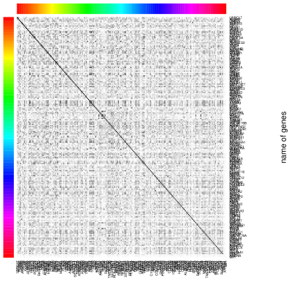
Figure 3: Sample covariance matrix

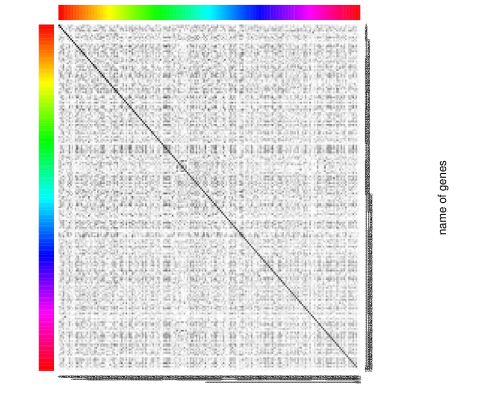
Figure 4: Estimated covariance matrix by LOREC

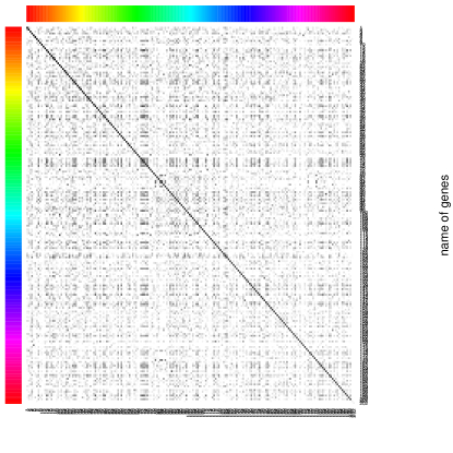
Figure 5: Estimated covariance matrix by PVD-based LOREC

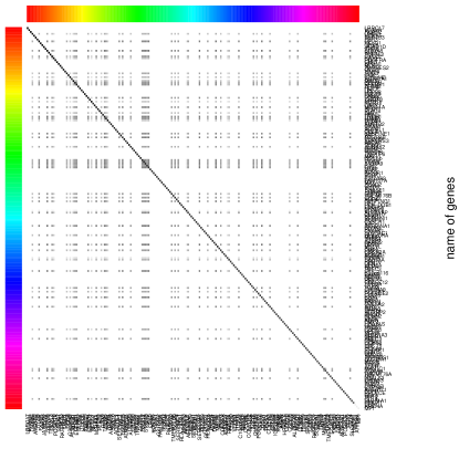
Figure 7: Estimated covariance matrix by PVD-based POET

Therefore, we start to perform PVD. First, we further consider genes with the first 200($p=200$) largest standard deviations from those genes whose SD is smaller than 1.5. The four methods: LOREC, PVD-based LOREC, POET and PVD-based POET are performed. When considering factor modelling, LOREC finds 10 common factors and the corresponding covariance matrix is similar to but slightly sparser than the ordinary sample covariance. When PVD is used, 47 pivotal genes are detected from these 200 genes, and then PVD-based LOREC finds 3 common factors. The corresponding covariance matrix is reasonably sparser than that obtained by LOREC. For both POET and PVD-based POET, only one common factor is considered and the corresponding covariance matrices are sparser than LOREC and PVD-based LOREC find. The corresponding heatmaps of the sample covariance matrix, and the estimated covariance matrices by LOREC, PVD-based LOREC, POET and PVD-based POET are respectively presented in Figures 3-7. It is clear that PVD helps on estimation and PVD-based POET can get sparser solution than all the competitors.

Figures 3-7 about here

7 Appendix

This subsection contains the proofs of the theorems 2 and 3 and proofs of other theorems are provided in Supplementary materia.

Proof of Theorem 2     Theorem 1 shows that under Condition (A2) and (A3), $\max\limits_{1\leq i\leq p}|\hat{r}_{i}-r_{i}|\leq C_{0}q_{n}$, with a probability $1-O(p^{-\delta_{0}})$. Therefore, as $n\to\infty$ , with a probability tending to 1, we have $\max\limits_{j\in J^{c}}\hat{r}_{i}<\delta_{p}+C_{0}q_{n}$ and $\min\limits_{j\in J}\hat{r}_{i}\geq c_{p}-C_{0}q_{n}$. As $q_{n}\rightarrow 0$, it holds that $\delta_{p}/q_{n}\rightarrow 0$ and $c_{p}/q_{n}\rightarrow\infty$ by Conditions (A1). Consequently, we have $\max\limits_{j\in J^{c}}\hat{r}_{i}/\min\limits_{j\in J}\hat{r}_{i}=o_{p}(1)$. This completes the proof. $\blacksquare$

Proof of Theorem 3     Under Conditions (A1)-(A3), Theorem 1 shows that, with probability tending to 1,

$$\max_{1\leq i\leq p}|\hat{r}_{i}-r_{i}|<C_{0}q_{n}.$$ (7.1)

Suppose that $J=\{1,\cdots,s_{0}(p)\}=\cup_{m=1}^{M}J_{m}$, such that for each $J_{m}$, $r_{i}$ with $i\in J_{m}$ takes the same value. Noting that $r_{i}$’s are arranged in the descending order, we assume $J_{m}=\{j_{m-1}+1,\cdots,j_{m}\}$ where $0=j_{0}<j_{1}<\cdots<j_{M}=s_{0}(p)$. For $1\leq i\leq p$, let $(i)$ denote the index $i_{0}$ such that $\hat{r}_{i_{0}}=\hat{r}_{(i)}$. Then define the sets $\hat{J}_{m}=\{(j_{m-1}+1),\cdots,(j_{m})\}$, $m=1,\cdots,M$. By Condition (A1), $\max\limits_{i\in J}r_{i}/\min\limits_{i\in J}r_{i}=O(1)$ and $r_{i}=O(c_{p}),i\in J$ uniformly. Then we have for some $0<m_{1}<m_{2}<\infty$, such that $m_{1}<r_{i}/c_{p}<m_{2}$ or $m_{1}c_{p}<r_{i}<m_{2}c_{p}$ for any $1\leq i\leq s_{0}(p)$. Then together with (7.1), we have $P(m_{1}c_{p}-C_{0}q_{n}<\hat{r}_{i}\leq m_{2}c_{p}+C_{0}q_{n},1\leq i\leq s_{0}(p))\rightarrow 1.$ By Condition (A1), we have $\max\limits_{i\in J^{c}}r_{i}\leq m_{3}\delta_{p}$ for some $0<m_{3}<\infty$. Then (7.1) yields that $P(\max_{i>s_{0}(p)}\hat{r}_{i}\leq m_{3}\delta_{p}+C_{0}q_{n})\rightarrow 1.$ Let $A_{n}=\{\cup_{m=1}^{M}\hat{J}_{m}=\cup_{m=1}^{M}J_{m}\}$. Combing the two formulas above with the fact that $\max(\delta_{p},q_{n})=o(c_{p})$, we have $P(A_{n})\rightarrow 1$, that is, the index set $\{(i),1\leq i\leq s_{0}(p)\}$ are consistent estimate of $J$.

Next we estimate $s_{0}(p)$. By the definitions of $l_{n}$ in Theorem 3, $c_{p}$ and $q_{n}$ in Condition (A1) and the fact that $\hat{r}_{(i)}>0$, as $n\rightarrow\infty$, it follows that with a probability tending to 1

$$\min\limits_{1\leq i<s_{0}(p)}R_{i}=\min\limits_{1\leq i<s_{0}(p)}\frac{\hat{r}_{(i+1)}+l_{n}}{\hat{r}_{(i)}+l_{n}}\geq\frac{m_{1}c_{p}-C_{0}q_{n}+l_{n}}{m_{2}c_{p}+C_{0}q_{n}+l_{n}}\rightarrow m_{1}/m_{2}>0,$$

$$R_{s_{0}(p)}=\frac{\hat{r}_{(s_{0}(p)+1)}+l_{n}}{\hat{r}_{(s_{0}(p))}+l_{n}}<\frac{m_{3}\delta_{p}+C_{0}q_{n}+l_{n}}{m_{2}c_{p}+C_{0}q_{n}+l_{n}}\rightarrow 0,$$

$$\min\limits_{i>s_{0}(p)}R_{i}=\min\limits_{i>s_{0}(p)}\frac{\hat{r}_{(i+1)}+l_{n}}{\hat{r}_{(i)}+l_{n}}\geq\frac{l_{n}}{m_{3}\delta_{p}+C_{0}q_{n}+l_{n}}\rightarrow 1,$$

where we have used the fact $\max(\delta_{p},q_{n})=o(l_{n})$ and $l_{n}=o(c_{p})$. Combining the above results with the definition of $\hat{s}_{0}(p)$ in (2.1), we have $P(\hat{s}_{0}(p)=s_{0}(p))\rightarrow 1.$ Further, recall that $P(A_{n})\rightarrow 1$ and that $\hat{J}=\{i:\hat{r}_{i}\geq\hat{r}_{(\hat{s}_{0}(p))}\}=\{(i):1\leq i\leq\hat{s}_{0}(p)\}$. Thus, we have $P(\hat{J}=J)\rightarrow 1$. This completes the proof. $\blacksquare$

References

12012Agarwal et al.Agarwal et al. (2012)Agarwal:2012 Agarwal, A., Negahban, S., and Wainwright, M. J. (2012). Noisy matrix decomposition via convex relaxation: Optimal rates in high dimensions. Annals of Statistics, 40, 1171-1197. 21993Bai and YinBai and Yin (1993)Bai:1993 Bai, Z. D., and Yin, Y. Q. (1993). Limit of the smallest eigenvalue of a large dimensional sample covariance matrix. Annals of Probability, 21, 1275–1294. 32002Bai and NgBai and Ng (2002)Bai:2002 Bai, J., and Ng, S. (2002). Determining the number of factors in approximate factor models. Econometrica, 70, 191-221. 42003BaiBai (2003)Bai:2003 Bai, J. (2003). Inferential theory for factor models of large dimensions. Econometrica, 71, 135-171. 52012Bai and LiBai and Li (2012)Bai:2012 Bai, J., and Li, K. (2012). Statistical analysis of factor models of high dimension. The Annals of Statistics, 40, 436-465. 62008Bickel and Levina Bickel and Levina (2008)Bickel:2008 Bickel, P. and Levina, E. (2008). Covariance regularization by thresholding. Annals of Statistics 36, 2577–2604. 72011Cai and LiuCai and Liu (2011)Cai:zhou:2012 Cai, T. T. and Liu, W. D. (2011). Adaptive thresholding for sparse covariance matrix estimation. Journal of the American Statistical Association, 106, 672–684. 82012Cai and Zhou Cai and Zhou (2012)Cai:zhou:2012 Cai, T. T. and Zhou, H. H. (2012). Optimal rates of convergence for sparse covariance matrix estimation. The Annals of Statistics, 40, 2389–2420. 92012Chandrasekaran et alChandrasekaran et al (2012)Chandrasekaran:2012 Chandrasekaran, V., Parrilo, P. A., nad Willsky, A. S. (2012). Latent Variable Graphical Model Selection via Convex Optimization. The Annals of Statistics, 40, 1935-1967. 102013Chen et al. Chen et al. (2013)Chen:etal:2013 Chen, X., Slack, F. J. and Zhao, H. (2013). Joint analysis of expression profiles from multiple cancers improves the identification of microRNA-gene interactions. Bioinformatics, 29, 2137–2145. 112008Fan et al Fan et al (2008)Fan:2008 Fan, J., Fan, Y., and Lv, J. (2008). High dimensional covariance matrix estimation using a factor model. Journal of Econometrics, 147, 186–197. 122011Fan et al. Fan et al. (2011)Fan:etal:2011 Fan, J., Liao, Y., and Mincheva, M. (2011). High-dimensional covariance matrix estimation in approximate factor models. The Annals of Statistics, 39, 3320–3356. 132013Fan et al Fan et al (2013)Fan:etal:2013 Fan, J., Liao, Y., and Mincheva, M. (2013). Large covariance estimation by thresholding principal orthogonal complements Journal of Royal Statistic Socociation, Series B, 75, 1–44. 142007Johnson et al. Johnson et al. (2007)Johnson:etal:2007 Johnson, W. E., Li, C., and Rabinovic, A. (2007). Adjusting batch effects in microarray expression data using empirical Bayes methods. Biostatistics, 8, 118–127. 152001Johnstone Johnstone (2001)Johnstone:2001 Johnstone, I. M. (2001). On the distribution of the largest eigenvalue in principal components analysis. The Annals of Statistics, 29, 295–327. 162011LuoLuo (2011)Luo:2011 Luo, X. (2011). High Dimensional Low Rank and Sparse Covariance Matrix Estimation via Convex Minimization. arXiv 1111.1133. 172011Ravikumar et al Ravikumar et al (2011)Ravikumar:2011 Ravikumar, P., Wainwright, M. J., Raskutti, G., and Yu, B. (2011). High-dimensional covariance estimation by minimizing ℓ1subscriptℓ1\ell_{1}-penalized log-determinant divergence. Electronic Journal of Statistics, 5, 935–980. 182009Rothman et al Rothman et al (2009)Rothman:2009 Rothman, A. J., Levina, E., and Zhu, J. (2009). Generalized thresholding of large covariance matrices. Journal of the American Statistical Association, 104, 177–186. 191980Serfling Serfling (1980)Serfling:1980 Serfling, R. J. (1980). Approximation theorems of mathematical statistics. Wiley series in probability and mathematical statistics. 201998Stock and WatsonStock and Watson (1998)Stock:1998 Stock, J. H., and Watson, M. W. (1998). Diffusion indexes Working Paper 6702. National Bureau of Economic Research, Cambridge. 212002Stock and WatsonStock and Watson (2002)Stock:2002 Stock, J. H., and Watson, M. W. (2002). Forecasting using principal components from a large number of predictors. Journal of the American statistical association, 97, 1167-1179. 222011VershyninVershynin (2011)Vershynin:2011 Vershynin, R. (2011). Introduction to the non-asymptotic analysis of random matrices. arXiv:1011.3027v5. 232013Xia et alXia et al (2013)Xia:2013 Xia, Q., Xu, W. L., and Zhu, L. X. (2014). Consistently determining the number of factors in multivariate volatility modelling. Statistica Sinica, accepted.

Table 1: Simulation results for $p=1000$

model	$p_{1}$	$\rho$	Mean	SD	FP	FN	EQ
		0.1	42.00	15.08	0.00	0.16	0.40
		0.3	50.07	0.30	0.00	0.01	0.94
	50	0.5	50.01	0.10	0.00	0.00	0.99
		0.7	50.01	0.10	0.00	0.00	0.99
		0.9	50.01	0.10	0.00	0.00	0.99
		0.1	65.42	44.92	0.00	0.35	0.19
		0.3	99.26	10.00	0.00	0.01	0.78
(1)	100	0.5	100.02	0.31	0.00	0.00	0.93
		0.7	100.10	0.48	0.00	0.00	0.94
		0.9	100.03	0.26	0.00	0.00	0.95
		0.1	117.51	109.73	0.01	0.45	0.02
		0.3	172.49	69.40	0.00	0.13	0.53
	200	0.5	198.38	10.95	0.00	0.01	0.78
		0.7	199.56	1.05	0.00	0.01	0.94
		0.9	200.10	0.30	0.00	0.00	0.98
		0.1	40.69	19.31	0.00	0.18	0.81
		0.3	48.35	8.34	0.00	0.03	0.90
	50	0.5	50.00	0.00	0.00	0.00	1.00
		0.7	50.00	0.00	0.00	0.00	1.00
		0.9	50.00	0.00	0.00	0.00	1.00
		0.1	82.75	37.18	0.00	0.17	0.41
		0.3	98.95	9.79	0.00	0.01	0.94
(2)	100	0.5	100.00	0.00	0.00	0.00	1.00
		0.7	100.00	0.00	0.00	0.00	1.00
		0.9	100.00	0.00	0.00	0.00	1.00
		0.1	122.12	96.28	0.00	0.38	0.24
		0.3	199.38	0.48	0.00	0.00	0.38
	200	0.5	200.00	0.00	0.00	0.00	1.00
		0.7	200.00	0.00	0.00	0.00	1.00
		0.9	200.00	0.00	0.00	0.00	1.00

Table 2: LOREC and PVD-based LOREC with the sample size $n=150$

			LOREC			PVD-based LOREC
$p$	$p_{1}$		$r$			$r$
			0.1	0.5	1	0.1	0.5	1
	20	EU	25.739	21.885	18.744	15.651	10.879	8.653
		RE	1.141	0.570	0.482	0.847	0.506	0.469
		TM	357.175	339.088	342.725	8.092	8.070	7.899
100	90	EU	18.632	13.669	11.908	6.452	4.335	1.533
		RE	1.053	0.502	0.450	0.801	0.479	0.448
		TM	317.930	347.613	365.470	234.173	248.974	267.590
	20	EU	32.825	25.356	21.172	15.935	10.298	7.772
		RE	1.463	0.607	0.534	0.772	0.516	0.490
		TM	1899.971	1759.109	2273.945	8.717	7.919	7.853
200	120	EU	30.485	10.238	5.651	9.189	4.033	3.534
		RE	1.242	0.571	0.514	0.811	0.429	0.411
		TM	1770.551	1766.879	1896.734	443.369	446.668	486.941
	20	EU	35.565	25.956	22.166	14.773	9.121	8.057
		RE	1.591	0.627	0.572	0.709	0.522	0.483
		TM	2750.761	2744.443	2894.143	8.842	8.742	8.537
300	120	EU	32.152	11.040	6.036	8.709	3.847	3.605
		RE	1.368	0.597	0.551	0.673	0.463	0.454
		TM	5238.465	5430.726	6050.430	457.111	511.934	509.842

Figure 1: Plots (a)–(c) present the average RE and plot (d)–(f) present the average EU for different values of $r$. In each plot, the solid line represents the results for POET and the dotted line for PVD-based POET.

Figure 2: The number of pivotal genes selected in T=50 replicas

Figure 6: Estimated covariance matrix by POET