Rotating Taylor-Green Flow

Abstract

The steady state of a forced Taylor-Green flow is investigated in a rotating frame of reference. The investigation involves the results of 184 numerical simulations for different Reynolds number $\mathrm{Re}_{{}_{F}}$ and Rossby number $\mathrm{Ro}_{{}_{F}}$. The large number of examined runs allows a systematic study that enables the mapping of the different behaviors observed to the parameter space ($\mathrm{{Re}}_{{}_{F}},\mathrm{{Ro}}_{{}_{F}}$), and the examination of different limiting procedures for approaching the large $\mathrm{Re}_{{}_{F}}$ small $\mathrm{Ro}_{{}_{F}}$ limit. Four distinctly different states were identified: laminar, intermittent bursts, quasi-2D condensates, and weakly rotating turbulence. These four different states are separated by power-law boundaries $\mathrm{Ro}_{{}_{F}}\propto\mathrm{Re}_{{}_{F}}^{-\gamma}$ in the small $\mathrm{Ro}_{{}_{F}}$ limit. In this limit, the predictions of asymptotic expansions can be directly compared to the results of the direct numerical simulations. While the first order expansion is in good agreement with the results of the linear stability theory, it fails to reproduce the dynamical behavior of the quasi-2D part of the flow in the nonlinear regime, indicating that higher order terms in the expansion need to be taken in to account. The large number of simulations allows also to investigate the scaling that relates the amplitude of the fluctuations with the energy dissipation rate and the control parameters of the system for the different states of the flow. Different scaling was observed for different states of the flow, that are discussed in detail. The present results clearly demonstrate that the limits small Rossby and large Reynolds do not commute and it is important to specify the order in which they are taken.

1 Introduction

An incompressible flow under rotation will experience the effect of the Coriolis force altering its dynamical behavior (Greenspan, 1968). At sufficiently high rotation rates it will suppress the velocity gradients along the direction of rotation bringing the flow in a quasi-2D state in which the flow varies only along two dimensions. This behavior is due to the Taylor-Proudman theorem obtained for flows which the eddy turn over time is much longer than the rotation period. In addition to rendering the flow quasi-2D a fast rotating system supports inertial waves whose frequency increases linearly with the rotation rate. Their fast dispersive dynamics weaken the nonlinear interactions allowing for some analytical treatment in the framework of weak wave turbulence theory (Nazarenko, 2011; Galtier, 2003). The interplay of the two phenomena quasi-2D and wave-turbulence can lead to a plethora of phenomena, often observed in natural flows.

Many different situations can be considered for rotating fluids that can lead to distinct results depending on the forcing mechanism, and the value of the involved control parameters. For example, different results can be envisioned for forced turbulence if the forcing mechanism injects energy exclusively to the quasi-2D component of the flow or if the forcing injects energy solely to the inertial waves. Differences are also expected if the domain size is increased and more dynamical wavenumbers are introduced in the system. The presence of helicity has also been shown to affect the behavior of the forward cascade (Teitelbaum & Mininni, 2009).

The large number of different possibilities has led to the emergence of numerous experimental and numerical studies. These studies of rotating turbulence although numerous, they have to face among other challenges this wide parameter space and different experimental setups have been considered. First experiments in rotating tanks date back to Hopfinger et al. (1982). Since then, numerous experiments have been constructed expanding the range of parameter space covered (Boubnov & Golitsyn, 1986; Sugihara et al., 2005; Ruppert-Felsot et al., 2005; Morize et al., 2005; Morize & Moisy, 2006; Davidson et al., 2006; Bewley et al., 2007; Staplehurst et al., 2008; van Bokhoven et al., 2009; Kolvin et al., 2009; Lamriben et al., 2011; Yarom et al., 2013). The increase of computational power has also allowed the study of rotating flows by simulations. Most numerical investigations have focused in decaying turbulence (Bardina et al., 1985; Mansour et al., 1992; Hossain, 1994; Bartello et al., 1994; Squires et al., 1994; Godeferd & Lollini, 1999; Smith & Waleffe, 1999; Morinishi et al., 2001; Müller & Thiele, 2007; Thiele & Müller, 2009; Teitelbaum & Mininni, 2010; Yoshimatsu et al., 2011), with more recent investigations of forced rotating turbulence both at large scales (Yeung & Zhou, 1998; Mininni et al., 2009; Mininni & Pouquet, 2009, 2010; Mininni et al., 2012) and at small scales in order to observe a development of an inverse cascade (Smith & Waleffe, 1999; Teitelbaum & Mininni, 2009; Mininni & Pouquet, 2009). Computational cost however did not allow for an exhaustive coverage of the parameter space. Small viscosity fluids (large Reynolds numbers) and high rotation rates (small Rossby numbers) put strong restrictions to simulations. Thus typically either moderate Reynolds numbers and small Rossby numbers are reached or moderate Rossby numbers and large Reynolds. Additionally, these runs have not reached a steady state that requires long integration times.

The present work attempts to overcome some of these limitations by focusing in one particular forcing mechanism and varying systematically the rotation rate and the viscosity. The aim is to understand and map the parameter space of a forced rotating flow. Thus the focus here is on a large number of simulations at moderate resolutions rather than a few high resolution runs. The object of the study is the steady state of a flow in a triple periodic square box of side $2\pi L$ forced by a body force ${\bf F}=F_{0}{\bf f}$ of forcing amplitude $F_{0}$ in the presence of rotation $\Omega$ in the ${\bf z}$-direction. To the authors knowledge this is the first study of forced rotating flows in the steady state. In this setup the Navier-Stokes equations for a unit density fluid with viscosity $\nu$ non-dimensionalized by the forcing amplitude $F_{0}$ and the box size $L$ are:

$$\partial_{t}{\bf u}=\mathbb{P}\left[{\bf u\times w}\right]+\mathrm{{Ro}}_{{}_{F}}^{-1}\mathbb{P}\left[{\bf u\times e_{z}}\right]+\mathrm{{Re}}_{{}_{F}}^{-1}\Delta{\bf u}+{\bf f},$$ (1)

${\bf u}$ is the velocity field (measured in units of $\sqrt{F_{0}L}$) satisfying $\nabla\cdot{\bf u}=0$. The vorticity field is given by ${\bf w=\nabla\times u}$. The unit vector in the $z$-direction is ${\bf e_{z}}$ and $\mathbb{P}$ is the projection operator to solenoidal fields that in the examined triple periodic domain can be written as

$$\mathbb{P}[{\bf g}]\equiv-\Delta^{-1}\nabla\times\nabla\times{\bf g}={\bf g}-\nabla\Delta^{-1}(\nabla\cdot{\bf g})$$ (2)

with $\Delta^{-1}$ being the inverse Laplace operator. The term $\nabla\Delta^{-1}(\nabla\cdot{\bf g})$ in 2 is equivalent to a pressure gradient term $\nabla P$ that guaranties incompressibility. The two control parameters in equation 1 are given by $\mathrm{{Re}}_{{}_{F}}\equiv\sqrt{F_{0}L}/\nu$ a Reynolds number based on the forcing amplitude, and $\mathrm{{Ro}}_{{}_{F}}\equiv\sqrt{F_{0}}/2\Omega\sqrt{L}$ a Rossby number based on the forcing amplitude. A more common choice for non-dimensionalization is the space time averaged squared velocity $U=\langle\langle{\bf u\cdot u}\rangle_{{}_{V}}\rangle_{{}_{T}}^{1/2}$, where here the angular brackets stand for space and time average.

$$\langle f\rangle_{{}_{V}}\equiv\frac{1}{(2\pi)^{3}}\int_{0}^{2\pi}\int_{0}^{2\pi}\int_{0}^{2\pi}f\,\,dxdydz,\qquad\langle f\rangle_{{}_{T}}\equiv\lim_{T\to\infty}\frac{1}{T}\int_{0}^{T}f\,\,dt.$$ (3)

Using $U$ we can obtain the usual definitions of the Reynolds $\mathrm{{Re}}_{{}_{U}}$ and Rossby $\mathrm{{Ro}}_{{}_{U}}$ number as $\mathrm{{Re}}_{{}_{U}}=\mathrm{{Re}}_{{}_{F}}U$ and $\mathrm{{Ro}}_{{}_{U}}=\mathrm{{Ro}}_{{}_{F}}U$. We note however that $\mathrm{Re_{{}_{U}}}$ and $\mathrm{Ro_{{}_{U}}}$ are not true control parameters of the examined dynamical system, since they are measured a posteriori. They are connected to the true control parameters $\mathrm{{Re}}_{{}_{F}},\mathrm{{Ro}}_{{}_{F}}$ by a map that needs however to be determined. As it turns out the map from the pair ($\mathrm{{Re}}_{{}_{F}},\mathrm{{Ro}}_{{}_{F}}$) to ($\mathrm{{Re}}_{{}_{U}},\mathrm{{Ro}}_{{}_{U}}$) is neither unique (for the same ($\mathrm{{Re}}_{{}_{F}},\mathrm{{Ro}}_{{}_{F}}$) two different states with different ($\mathrm{{Re}}_{{}_{U}},\mathrm{{Ro}}_{{}_{U}}$) exist) nor onto ( not all pairs of ($\mathrm{{Re}}_{{}_{U}},\mathrm{{Ro}}_{{}_{U}}$) can be obtained by a suitable choice of ($\mathrm{{Re}}_{{}_{F}},\mathrm{{Ro}}_{{}_{F}}$).)

A third choice for non-dimensionalization is the energy dissipation rate $\epsilon$ that is defined as

$$\epsilon\equiv\mathrm{{Re}}_{{}_{F}}^{-1}\langle\langle{\bf w\cdot w}\rangle_{{}_{V}}\rangle_{{}_{T}}=\langle\langle{\bf f\cdot u}\rangle_{{}_{V}}\rangle_{{}_{T}}.$$ (4)

The last equality is due to the energy conservation property of the nonlinear and the rotation term. The new parameters that can be defined are $\mathrm{Re_{{}_{D}}}=\mathrm{Re_{{}_{F}}}\epsilon^{1/3}$ and $\mathrm{Ro_{{}_{D}}}=\mathrm{Ro_{{}_{F}}}\epsilon^{1/3}$. This choice of control parameters is mostly met in theoretical investigations (like weak wave turbulence theory). As with the case of ($\mathrm{{Re}}_{{}_{U}},\mathrm{{Ro}}_{{}_{U}}$), the parameters based on the energy dissipation ($\mathrm{{Re}}_{{}_{D}},\mathrm{{Ro}}_{{}_{D}}$), can only be determined a posteriori and are not true control parameters. They do provide however a better measure of the strength of turbulence than the other two definitions. The three choices of control parameter pairs can be summarized as $Re=\mathcal{U}L/\nu$, $Ro=\mathcal{U}/(2\Omega L)$ where the dimensional velocity $\mathcal{U}$ corresponds to the choice $\mathcal{U}=\sqrt{F_{0}L}$ for ($\mathrm{{Re}}_{{}_{F}},\mathrm{{Ro}}_{{}_{F}}$), $\mathcal{U}=\langle\tilde{u}^{2}\rangle_{{}_{V}}^{1/2}$ for ($\mathrm{{Re}}_{{}_{U}},\mathrm{{Ro}}_{{}_{U}}$) and $\mathcal{U}=(\tilde{\epsilon}L)^{1/3}$ for ($\mathrm{{Re}}_{{}_{D}},\mathrm{{Ro}}_{{}_{D}}$), where $\tilde{u}$ and $\tilde{\epsilon}$ the dimensional velocity and energy dissipation rate respectively.

The flow in this study is forced by the Taylor-Green (TG) vortex at wavenumber $q$:

$${\bf f}=2\left\{\begin{array}[]{ll}&{\bf e_{x}}\,\,\sin(qx)\cos(qy)\sin(qz)\\ -&{\bf e_{y}}\,\,\cos(qx)\sin(qy)\sin(qz)\\ &{\bf e_{z}}\,\,0\end{array}\right..$$ (5)

It is normalized so that $\langle{\bf f\cdot f}\rangle_{{}_{V}}^{1/2}=1$. Taylor-Green is a archetypal example of a nonhelical flow that leads to a fast generation of small scale structures and has been one of the first examples to study as a candidate for finite time singularity of the Euler equations (Brachet et al., 1992). Due to its simplicity it has served as a model of many laboratory flows (Maurer & Tabeling, 1998; Monchaux et al., 2007, 2009; Cortet et al., 2010; Salort et al., 2010). It has also been used as forcing in simulations for the study of non-helical hydrodynamic turbulent flows (Mininni et al., 2006) and rotating flows (Mininni et al., 2009; Mininni & Pouquet, 2009; Teitelbaum & Mininni, 2009). Finally it has been studied for its magnetic dynamo properties due to its similarities with laboratory dynamo experiments (Ponty et al., 2008).

This study investigates the properties of a TG forced flow, varying both the rotation rate and the Reynolds number, covering the two dimensional parameter space.

2 Parameter space - Phase diagram

The numerical part of our study consists of 184 direct numerical simulations of the Navier-Stokes equations 1 varying the values of the control parameters $\mathrm{{Re}}_{{}_{F}}$ and $\mathrm{{Ro}}_{{}_{F}}$. For all runs the forcing wave-number was kept fixed to $q=2$. All runs were performed using a standard pseudo-spectral code, where each component of $\bm{u}$ and $\bm{b}$ is represented as truncated Galerkin expansion in terms of the Fourier basis. The nonlinear terms are initially computed in physical space and then transformed to spectral space using fast-Fourier transforms. Aliasing errors are removed using the 2/3 de-aliasing rule. The temporal integration was performed using a fourth-order Runge-Kutta method. Further details on the code can be found in (Gómez et al., 2005). The grid size varied depending on the value of $\mathrm{{Re}}_{{}_{F}}$ and $\mathrm{{Ro}}_{{}_{F}}$ from to $64^{3}$ to $512^{3}$. A run was considered well resolved if the value of enstrophy spectrum at the cut-off wavenumber was more than an order of magnitude smaller than its value at its peak. Each run started from random multi-mode initial conditions and was continued for sufficiently long time so that long time averages in the steady state were be obtained.

Figure 1: Left panel: The parameter space $(\mathrm{{Ro}}_{{}_{F}},\mathrm{{Re}}_{{}_{F}}$). Each point in this plane indicates a numerical simulation with this choice of parameters ($\mathrm{{Re}}_{{}_{F}},\mathrm{{Ro}}_{{}_{F}}$). Different symbols indicate different behavior: laminar flows are indicated by squares, intermittent bursts are indicated by triangles, quasi-2D condensates are indicated by circles, weakly rotating flows are indicated by diamonds. The different shades of gray (colors online) used are indicative of the magnitude of $\mathrm{{Ro}}_{{}_{F}}$. Large symbols imply larger value of $\mathrm{{Re}}_{{}_{F}}$. Right panel: Energy evolution for four representative cases.

The location of all the performed runs in the ($\mathrm{{Re}}_{{}_{F}},\mathrm{{Ro}}_{{}_{F}}$) parameter space are shown in the first panel of figure 1. The set of data with the largest value of $\mathrm{{Ro}}_{{}_{F}}$ are in reality non-rotating runs ($\mathrm{{Ro}}_{{}_{F}}=\infty$) that have been shifted to the finite value $\mathrm{{Ro}}_{{}_{F}}=8$ so that they can appear in a logarithmic diagram. The different shades of gray (colors online) used are indicative of the magnitude of $\mathrm{{Ro}}_{{}_{F}}$ (thus light colors (red online) imply slow rotation while dark colors (violet online) imply fast rotation. Large symbols imply larger value of $\mathrm{{Re}}_{{}_{F}}$. The same symbols, sizes and shades (colors online) are used in all subsequent figures and thus the reader can always refer to figure 1 to estimate the value of $\mathrm{{Re}}_{{}_{F}}$ and $\mathrm{{Ro}}_{{}_{F}}$. The different symbols indicate the four different behaviors that were observed in the numerical runs. Four representative cases of these behaviors are shown in the right panel of figure 1. All cases have the same value of $\mathrm{{Re}}_{{}_{F}}$ but different values of $\mathrm{{Ro}}_{{}_{F}}$. Note the differences in values in $y$-axis that indicate the different range of amplitude reached and the differences in values in $x$-axis that indicate the different time scales involved. The top sub-figure displays the evolution of energy from a run that displayed laminar behavior: after some transient period all energy is concentrated in the forcing scales and no fluctuations in the temporal behavior are observed. This behavior is observed in runs that occupy the lower and the left part of the shown parameter space and are indicated by squares $\Box$. The second from the top sub-figure displays a run for which the energy evolution displayed intermittent bursts. It consists of sudden bursts of energy followed by long relaxation periods reaching very small values of kinetic energy. In the left panel they are marked by triangles $\bigtriangleup$. They are found for low values of $\mathrm{{Ro}}_{{}_{F}}$ and high $\mathrm{{Re}}_{{}_{F}}$. Note that triangles and squares sometimes overlap indicating a bimodal behavior of the flow. The third from the top sub-figure shows the energy evolution from a run that formed quasi-2D condensates. The energy in these cases reaches very high values and it is concentrated in a few large scale 2D-modes (ie $k_{z}=0$, $k_{x}\sim k_{y}\sim 1$). They a represented in the left panel by circles $\bigcirc$. They appear for intermediate values of $\mathrm{{Ro}}_{{}_{F}}$ and for large $\mathrm{{Re}}_{{}_{F}}$. Finally the bottom sub-figure in 1 displays the results from a weakly rotating flow. The behavior of these flows as the name suggests weakly deviates from the non-rotating ones: energy saturates at order one values and only weak anisotropy is observed. They are represented by diamonds $\Diamond$ in the left panel and occupy the higher and right part of the parameter space.

The dashed lines in the left panel of figure 1 separate the parameter space to the different phases that are observed. The parameter space is then split in 5 different regions: laminar, laminar and bursts, bursts, quasi 2D condensates, and weakly rotating flow. For large values of $\mathrm{{Re}}_{{}_{F}}$ and $\mathrm{{Ro}}_{{}_{F}}$ these boundaries are expected to take the form of power laws. Indeed this assumption seems reasonable given the data. The scaling $\mathrm{{Ro}}_{{}_{F}}\propto\mathrm{{Re}}_{{}_{F}}^{-1}$ seems to determine the boundary that separates laminar region from the bursts and laminar bimodal behavior. The region that exhibits quasi-2D condensates is bounded from below by a weak power law $\mathrm{{Ro}}_{{}_{F}}\propto\mathrm{{Re}}_{{}_{F}}^{-\alpha}$. The value of $\alpha$ however cannot be determined by the present data. The difficulty in resolving both high $\mathrm{{Re}}_{{}_{F}}$ and high $\mathrm{{Ro}}_{{}_{F}}$ limits us only to a qualitative estimate of this lower boundary and prohibits us from measuring precisely $\alpha$. We will attempt however to argue the origin of these power laws in the following sections using scaling arguments and asymptotic expansions. From above the quasi 2D condensates appear to be bounded by the value $\mathrm{{Ro}}_{{}_{F}}\simeq 0.4$ and appear only for $\mathrm{{Re}}_{{}_{F}}>240$. For larger values of $\mathrm{{Ro}}_{{}_{F}}$ weakly rotating flows are observed.

Figure 2: The Parameter Space $(\mathrm{{Ro}}_{{}_{U}},\mathrm{{Re}}_{{}_{U}}$) in the left and $(\mathrm{{Ro}}_{{}_{D}},\mathrm{{Re}}_{{}_{D}}$) in the right. Each point in this plane indicates a numerical simulation that resulted in that value of $(\mathrm{{Ro}}_{{}_{U}},\mathrm{{Re}}_{{}_{U}})$ and $(\mathrm{{Ro}}_{{}_{D}},\mathrm{{Re}}_{{}_{D}}$). Same symbols are used for the same runs as in figure 1.

As mentioned in the previous section the definition of the Reynolds and Rossby number is more than just a conventional formality in rotating turbulence. In figure 2 we show the data in the parameter space $(\mathrm{{Re}}_{{}_{U}},\mathrm{{Ro}}_{{}_{U}})$ in the left panel and in the paramater space $(\mathrm{{Re}}_{{}_{D}},\mathrm{{Ro}}_{{}_{D}})$ in the right panel. The presence of large scale condensates and the suppression of turbulence by rotation drastically alters the range covered by the simulations for the different parameter choice. In the ($Re_{{}_{U}}$, $Ro_{{}_{U}}$) parameter space the data appear more scattered. In particular the subcritical transition from laminar to intermittent bursts has lead to the to a region vacant of points around $\mathrm{{Ro}}_{{}_{U}}=10^{-2},\mathrm{{Re}}_{{}_{U}}=100$ and $\mathrm{{Ro}}_{{}_{D}}=10^{-2},\mathrm{{Re}}_{{}_{D}}=30$. The quasi 2D condensates also have lead extremely large values of $Re_{{}_{U}}$ to be reached. On the other hand in the ($Re_{{}_{D}}$, $Ro_{{}_{D}}$), the data seem to be much more concentrated and bounded on the right by $Re_{{}_{D}}\simeq 1000$. This only reflects the maximum grid size used $N=512^{3}$. Thus $Re_{{}_{D}}$ provides the best measure for the range of scales excited and therefor on how turbulent is the flow is. In the following sections however the data will be presented based on the parameters ($Re_{{}_{F}}$, $Ro_{{}_{F}}$) since these are the ones that are controlled in the numerical experiments.

3 Stationary solutions in the $\mathrm{{Ro}}_{{}_{F}}\to 0$ limit

The complex phase space observed can be disentangled by looking at the fast rotating limit in which the smallness of $\mathrm{{Ro}}_{{}_{F}}$ can be used to find asymptotic solutions. For $\mathrm{{Ro}}_{{}_{F}}\ll 1$ the first order term in 1 is linear and a solution can be obtained in terms of an expansion series treating the nonlinearity in a perturbative manner. We thus write ${\bf u}=\mathrm{{Ro}}_{{}_{F}}{\bf v}$ and expand ${\bf v}$ as

$${\bf v}={\bf v}^{(0)}+\mathrm{{Ro}}_{{}_{F}}^{2}\,\,{\bf v}^{(1)}+\mathrm{{Ro}}_{{}_{F}}^{4}\,\,{\bf v}^{(2)}+\dots$$ (6)

(The upper indices in parenthesis indicate order of the expansion and not powers.) As a first step we look for stationary solutions to the problem and thus assume no time dependence. It is further assumed the following scaling for the Reynolds number $\mathrm{{Re}}_{{}_{F}}^{-1}=\lambda_{n}\mathrm{{Ro}}_{{}_{F}}^{2n-1}$ where now $\lambda_{n}$ is an order one number and $n$ an integer to be specified. It determines the order at which the viscous term will appear in the expansion and thus it will be referred to as the ordering index. After substitution equation 1 becomes

$$\mathbb{L}\left[{\bf v}\right]={\bf f}+\mathrm{{Ro}}_{{}_{F}}^{2}\,\,\mathbb{P}\left[{\bf v\times w}\right]+\lambda_{n}\mathrm{{Ro}}_{{}_{F}}^{2n}\Delta{\bf u}.$$ (7)

where now ${\bf w=\nabla\times v}$. The linear operator $\mathbb{L}$ on the left hand side expresses the effect of rotation and is defined as

$$\mathbb{L}\left[{\bf v}\right]\equiv\mathbb{P}\left[{\bf e_{z}}\times{\bf v}\right].$$ (8)

In the triple periodic domain $\mathbb{L}$ can be written as:

$$\mathbb{L}[{\bf f}]=\Delta^{-1}\partial_{z}\nabla\times{\bf f}$$ (9)

Its kernel is composed of all solenoidal vector fields ${\bf g}$ such that $\partial_{z}{\bf g}=0$. These vector fields are going to be referred to as two-dimensional-three-components (2D3C) fields as they depend only on two coordinates but involve all three components. The projection to the 2D3C-fields is just the vertical average that is denoted as

$$\overline{\bf g}\equiv\frac{1}{2\pi}\int_{0}^{2\pi}{\bf g}\,\,\,dz$$ (10)

For any ${\bf f}$ that has zero projection in this set ($ie$ $\overline{\bf f}=0$) the general solution to the equation $\mathbb{L}{\bf g}={\bf f}$ is:

$${\bf g}=\mathbb{L}^{-1}{\bf f}+{\bf g}_{{}_{2D}}=-\partial_{z}^{-1}\nabla\times{\bf f}+{\bf g}_{{}_{2D}}$$ (11)

where ${\bf g}_{{}_{2D}}$ is an arbitrary (2D3C) field. If however $\overline{\bf f}\neq 0$ no solution exists.

Equation 7 can be treated perturbatively and a stationary ${\bf v}$ can in principle be found as a series expansion in $\mathrm{{Ro}}_{{}_{F}}^{2}$. Since the Taylor-Green flow is not a solution of the Euler equations at each order new wavenumbers will be excited. This procedure will terminate by viscosity that will introduce an exponential cutoff. It is not a surprise then that the ordering parameter $n$ that controls the relation between $\mathrm{{Re}}_{{}_{F}}$ and $\mathrm{{Ro}}_{{}_{F}}$ also controls the convergence of the expansion. Thus the investigation begins by examining different possible values of the ordering parameter $n$.

3.1 $n=0$, $\mathrm{{Re}}_{{}_{F}}^{-1}=\lambda_{0}\mathrm{{Ro}}_{{}_{F}}^{-1}$

For $n=0$ the viscous term is of the same order with the rotation term and the operator that needs to be inverted to obtain the first order term in ${\bf v}$ is $(\mathbb{L}-\lambda_{0}\Delta)$. This operator is positive definite and can always be inverted to obtain the zeroth order solution. In detail for the Taylor-Green forcing eq. (5) it is obtained that

$${\bf v^{(0)}}=\frac{2}{1+27\lambda_{0}^{2}q^{4}}\left\{\begin{array}[]{lcl}{\bf e_{x}}(-\cos(qx)\sin(qy)\sin(qz)&+9\lambda_{0}q^{2}\sin(qx)\cos(qy)\sin(qz)&)\\ {\bf e_{y}}(-\sin(qx)\cos(qy)\sin(qz)&-9\lambda_{0}q^{2}\cos(qx)\sin(qy)\sin(qz)&)\\ {\bf e_{z}}(\,2\,\sin(qx)\sin(qy)\cos(qz)&&)\end{array}\right..$$ (12)

The next order correction follows in a similar manner without a qualitative change the of the flow behavior. We note that the stationary solution in this limit follows the scaling $\langle{\bf u\cdot u}\rangle_{{}_{V}}=\mathrm{{Ro}}_{{}_{F}}^{2}\langle{\bf v\cdot v}\rangle_{{}_{V}}=3\mathrm{{Ro}}_{{}_{F}}^{2}(1+27\lambda_{0}^{2}q^{4})^{-1}$. That implies that the relation between $(\mathrm{{Re}}_{{}_{U}},\mathrm{{Ro}}_{{}_{U}})$ and $(\mathrm{{Re}}_{{}_{F}},\mathrm{{Ro}}_{{}_{F}})$ for the laminar flow is given by

$$\mathrm{{Re}}_{{}_{U}}=\frac{\sqrt{3}\,\mathrm{{Re}}_{{}_{F}}^{2}\mathrm{{Ro}}_{{}_{F}}}{\sqrt{\mathrm{{Re}}_{{}_{F}}^{2}+27\mathrm{{Ro}}_{{}_{F}}^{2}q^{4}}},\qquad\mathrm{{Ro}}_{{}_{U}}=\frac{\sqrt{3}\,\mathrm{{Ro}}_{{}_{F}}^{2}\mathrm{{Re}}_{{}_{F}}}{\sqrt{\mathrm{{Re}}_{{}_{F}}^{2}+27\mathrm{{Ro}}_{{}_{F}}^{2}q^{4}}},$$ (13)

Furthermore, $\langle{\bf u\cdot f}\rangle=9q^{2}\mathrm{{Ro}}_{{}_{F}}\lambda_{0}(1+27\lambda_{0}^{2}q^{4})^{-1}$ and thus

$$\mathrm{{Re}}_{{}_{D}}=\frac{3^{2/3}\,\mathrm{{Re}}_{{}_{F}}^{4/3}\mathrm{{Ro}}_{{}_{F}}^{1/3}}{(\mathrm{{Re}}_{{}_{F}}^{2}+27\mathrm{{Ro}}_{{}_{F}}^{2}q^{4})^{1/3}},\qquad\mathrm{{Ro}}_{{}_{D}}=\frac{3^{2/3}\,\mathrm{{Ro}}_{{}_{F}}^{4/3}\mathrm{{Re}}_{{}_{F}}^{1/3}}{(\mathrm{{Re}}_{{}_{F}}^{2}+27\mathrm{{Ro}}_{{}_{F}}^{2}q^{4})^{1/3}},$$ (14)

These results 13,14 provide the map from the $(\mathrm{{Re}}_{{}_{U}},\mathrm{{Ro}}_{{}_{U}})$ space (left panel of figure 1) to the $(\mathrm{{Re}}_{{}_{U}},\mathrm{{Ro}}_{{}_{U}})$ and $(\mathrm{{Re}}_{{}_{D}},\mathrm{{Ro}}_{{}_{D}})$ space shown in figure 2 but only for the laminar solutions.

3.2 $n=1$, $\mathrm{{Re}}_{{}_{F}}^{-1}=\lambda_{1}\mathrm{{Ro}}_{{}_{F}}^{1}$

For this value of the ordering index, equation 7 becomes

$$\mathbb{L}\left[{\bf v}\right]={\bf f}+\mathrm{{Ro}}_{{}_{F}}^{2}\,\,(\mathbb{P}\left[{\bf v\times w}\right]+\lambda_{1}\Delta{\bf u}).$$ (15)

Since $\overline{\bf f}=0$ the zeroth order solution can be written as ${\bf v}^{(0)}={\bf v}^{(0)}_{\bf f}+{\bf v}_{{}_{2D}}^{(0)}$ where

$${\bf v}^{(0)}_{\bf f}=\mathbb{L}^{-1}{\bf f}=2\left\{\begin{array}[]{lcl}-&{\bf e_{x}}&\cos(qx)\sin(qy)\sin(qz)\\ -&{\bf e_{y}}&\sin(qx)\cos(qy)\sin(qz)\\ 2&{\bf e_{z}}&\sin(qx)\sin(qy)\cos(qz)\end{array}\right.,$$ (16)

and ${\bf v}_{{}_{2D}}^{(0)}$ is an arbitrary 2D3C field. The velocity field in eq.16 is the same as the one in 12 with $\lambda_{0}=0$. The 2D3C field is determined at next order for which we have

$$\mathbb{L}[{\bf v}^{(1)}]=\mathbb{P}\left[{\bf v}^{(0)}\times{\bf w}^{(0)}\right]+\lambda_{1}\Delta{\bf v}^{(0)}.$$ (17)

Averaging over the $z$ direction we obtain by detailed calculation that:

$$\overline{\mathbb{P}\left[{\bf v}^{(0)}_{f}\times{\bf w}_{{}_{2D}}^{(0)}\right]}=\overline{\mathbb{P}\left[{\bf v}_{{}_{2D}}^{(0)}\times{\bf w}_{f}^{(0)}\right]}=\overline{\mathbb{P}\left[{\bf v}^{(0)}_{f}\times{\bf w}^{(0)}_{f}\right]}=0$$ (18)

where ${\bf w}_{{}_{2D}}^{(0)}=\nabla\times{\bf v}_{{}_{2D}}^{(0)}$ and ${\bf w}^{(0)}_{\bf f}=\nabla\times{\bf v}^{(0)}_{\bf f}$. We are thus left with:

$$0=\mathbb{P}\left[{\bf v}_{{}_{2D}}^{(0)}\times{\bf w}^{(0)}_{{}_{2D}}\right]+\lambda_{1}\Delta{\bf v}_{{}_{2D}}^{(0)}.$$ (19)

Multiplying by ${\bf v}_{{}_{2D}}^{(0)}$ and horizontal averaging we get $\langle{(\nabla{\bf v}_{{}_{2D}}^{(0)})}^{2}\rangle_{{}_{V}}=0$ and thus the undetermined 2D3C field at first order becomes ${\bf v}_{{}_{2D}}^{(0)}=0$. A 2D3C flow can possibly appear at higher order but we will proceed no further than obtaining ${\bf v}^{(0)}$.

The relations given in 13 simplify (by setting $\lambda_{0}=0$) to

$$\mathrm{{Re}}_{{}_{U}}=\sqrt{3}\,\mathrm{{Re}}_{{}_{F}}\mathrm{{Ro}}_{{}_{F}}\quad\mathrm{and}\quad\mathrm{{Ro}}_{{}_{U}}=\sqrt{3}\,\mathrm{{Ro}}_{{}_{F}}^{2}$$ (20)

for the Reynolds numbers based on the root mean square velocity. Similarly 14 simplify to $\mathrm{{Re}}_{{}_{D}}=3^{2/3}\,\mathrm{{Re}}_{{}_{F}}^{1/3}\mathrm{{Ro}}_{{}_{F}}^{2/3}$ and $\mathrm{{Ro}}_{{}_{D}}=3^{2/3}\,\mathrm{{Re}}_{{}_{F}}^{-1/3}\mathrm{{Ro}}_{{}_{F}}^{4/3}$ for the Reynolds numbers based on the energy injection rate.

3.3 $n=2$, $\mathrm{{Re}}_{{}_{F}}^{-1}=\lambda_{2}\mathrm{{Ro}}_{{}_{F}}^{3}$

For this ordering index the expansion follows as before but viscosity is not present at first order and the solvability condition obtained in 17 only restricts ${\bf v}_{{}_{2D}}$ at being a solution of the Euler equations $\mathbb{P}\left[{\bf v}_{{}_{2D}}^{(0)}\times{\bf w}_{{}_{2D}}^{(0)}\right]=0$. The first order correction is then

$${\bf v}^{(1)}=\mathbb{L}^{-1}[{\bf v^{(0)}\times w^{(0)}}]+{\bf v}_{{}_{2D}}^{(1)}.$$ (21)

To proceed at second order and simplify the mathematical complexity that increases rapidly with the order of the expansion we will assume at this point that ${\bf v}_{{}_{2D}}=0$ and verify a posteriori the validity of this assumption. To the next order the we obtain

$$\mathbb{L}[{\bf v}^{(2)}]=\mathbb{P}\left[{\bf v}^{(1)}\times{\bf w}^{(0)}+{\bf v}^{(0)}\times{\bf w}^{(1)}\right]+\lambda_{2}\Delta{\bf v}^{(0)}.$$ (22)

Averaging over $z$ the nonlinear term drops to zero. This can be realized by noticing that the 0-th order components (${\bf v}^{(0)},{\bf w}^{(0)}$) only contain wavenumbers $\pm q$ in the $z$-direction while the first order component (${\bf v}^{(1)},{\bf w}^{(1)}$) has only $\pm 2q$ wavenumbers. Their product will thus have only $\pm q$ and $\pm 3q$ wave numbers and will thus average to zero. We obtain thus $\overline{\nabla^{2}\bf v^{(0)}}=0$ in agreement with our original assumption that ${\bf v}_{{}_{2D}}=0$. Up to this scaling therefore the stationary solution obtained has zero projection to the 2D3C fields.

3.4 $n=3$, $\mathrm{{Re}}_{{}_{F}}^{-1}=\lambda_{3}\mathrm{{Ro}}_{{}_{F}}^{5}$

The assumption that ${\bf v}_{{}_{2D}}=0$ ceases to be true for this ordering. If we assume that ${\bf v}^{0}_{{}_{2D}}=0$ then at third order where the dissipation term is present we will obtain

$$\mathbb{L}[{\bf v}^{(3)}]=\mathbb{P}\left[{\bf v}^{(2)}\times{\bf w}^{(0)}+{\bf v}^{(0)}\times{\bf w}^{(2)}+{\bf v}^{(1)}\times{\bf w}^{(1)}\right]+\lambda_{3}\Delta{\bf v^{(0)}}.$$ (23)

where ${\bf v}^{(0)},{\bf v}^{(1)}$ and ${\bf v}^{(2)}$ are obtained from eq. 16, 21 and 22 respectably with $\lambda_{2}=0$. Averaging over $z$ the nonlinear term will not become zero and thus will need to be balanced by the viscosity.

$$\lambda_{3}\nabla^{2}{\bf v_{{}_{2D}}}=\lambda_{3}\nabla^{2}\overline{\bf v^{(0)}}=-\overline{\mathbb{P}\left[{\bf v}^{(2)}\times{\bf w}^{(0)}+{\bf v}^{(0)}\times{\bf w}^{(2)}+{\bf v}^{(1)}\times{\bf w}^{(1)}\right]}\neq 0$$ (24)

Thus ${\bf v_{{}_{2D}}=0}$ is no longer an acceptable solution. Calculation of the nonlinear term 24 leads to

$$\overline{\mathbb{P}\left[{\bf v}^{(2)}\times{\bf w}^{(0)}+{\bf v}^{(0)}\times{\bf w}^{(2)}+{\bf v}^{(1)}\times{\bf w}^{(1)}\right]}=\left\{\begin{array}[]{r}\partial_{y}\Psi\\ -\partial_{x}\Psi\\ 0\end{array}\right\}$$ (25)

with

$$\Psi=\frac{9q}{2}[\cos(2qx)-\cos(2qy)]\sin(2qx)\sin(2qy)$$ (26)

Thus even if the initial data have a zero projection to the 2D3C fields the nonlinearity at third order will force a 2D3C component to grow to zeroth order amplitude.

3.5 $n>4$, $\mathcal{O}(\mathrm{{Re}}_{{}_{F}}^{-1})<\mathcal{O}(\mathrm{{Ro}}_{{}_{F}}^{5})$

At higher values of $n$ the nonlinearity at the 4th order term has non-zero projection to the 2D3C fields and viscosity is not present to provide a balance. Thus no solution can be obtained by the expansion. Physically this would imply that even if initial conditions were prepared carefully to avoid any instabilities the 2D3C component of the flow would grow with time to values where the original scaling ${\bf u}=\mathrm{{Ro}}_{{}_{F}}{\bf v}\ll 1$ would not be valid and the expansion would fail. This also indicates that the quasi-2D condensates that were shown in 1 will show up at this order. This gives a lower bound on the unknown exponent $\alpha\geq\frac{1}{5}$ since at this order there is direct injection of energy in the 2D3C flow.

4 Time evolution and stability in the $Ro_{{}_{F}}\to 0$ limit

The results in the previous section only imply the presence of stationary solutions. Their realizability however is not guarantied since it can be unstable to infinitesimal or finite amplitude perturbations that can lead the system to different time dependent solutions. It is thus also important to investigate the stability of the calculated solutions. To follow the evolution of the flow we need to keep the time derivative term in eq. 1. Since in rapidly rotating systems two distinct time scales exist one given by the rotation rate and one by the nonlinearity we introduce $\tau=\mathrm{{Ro}}_{{}_{F}}t$ as the slow eddie turn over time and $t^{\prime}=\mathrm{{Ro}}_{{}_{F}}^{-1}t$ as the fast time scale. Equation 1 then becomes

$$\partial_{t^{\prime}}{\bf v}+\mathbb{L}\left[{\bf v}\right]={\bf f}+\mathrm{{Ro}}_{{}_{F}}^{2}\,\,\mathbb{P}\left[-\partial_{\tau}{\bf v+v\times w}\right]+\lambda_{n}\mathrm{{Ro}}_{{}_{F}}^{2n}\Delta{\bf v}.$$ (27)

In principle this expansion remains valid only on the timescale $\tau$ and could fail at longer time scales (Newell, 1969; Babin et al., 1969; Chen et al., 2005). In practical terms however such expansions are expected to capture the long time dynamics (eg saturation amplitude, dissipation rates ect) if slower time scale processes in the system do not become important. If such a third timescale exist the expansion should be carried out at the next order and a new timescale to be defined.

In addition to the stationary solution that was found in the previous section, the time dependence allows for the existence of traveling inertial waves that propagate on the fast time scale $t^{\prime}$ and vary in amplitude on the slow dynamical time scale $\tau$. The presence of the inertial waves (since they are not directly forced) depends on their stability properties. Similar the 2D3C flows that are absent in the stationary solution for $\mathrm{{Re}}_{{}_{F}}\leq\mathcal{O}(\mathrm{{Ro}}_{{}_{F}}^{-3})$ can still be present as time dependent solutions evolving on slow time scale $\tau$ if an instability is present.

4.1 Energy stability

The energy stability method provides a sufficient criterion for stability of a stationary flow subject to perturbations of arbitrary amplitude. It is based on the energy evolution equation of the perturbation. Denoting the stationary solution as ${\bf u}_{f}$ and without taking any asymptotic limit yet we can write the velocity field ${\bf u}$ as the sum of the stationary solution ${\bf u}_{f}$ and a fluctuating part ${\bf u}_{p}$. Multiplying equation 1 by the fluctuating part ${\bf u}_{p}$ and space averaging leads to the equation

$$\frac{d}{dt}\left\langle\frac{1}{2}|{\bf u}_{p}|^{2}\right\rangle_{{}_{V}}=\left\langle{\bf u}_{p}\cdot\left(\nabla{\bf u}_{f}\right){\bf u}_{p}\right\rangle_{{}_{V}}-\mathrm{{Re}}_{{}_{F}}^{-1}\left\langle|\nabla{\bf u}_{p}|^{2}\right\rangle_{{}_{V}}.$$ (28)

The stationary solution is then called energy stable if the right hand side is negative definite for all incompressible fields ${\bf u}_{p}$. Note that the Coriolis term is absent in eq.28 and the same equation is obtained if $\mathrm{{Ro}}_{{}_{F}}=\infty$. However there is dependence on $\mathrm{{Ro}}_{{}_{F}}$ through the functional form of ${\bf u}_{f}$. Stability of the stationary solution is then guarantied if

$$\mu(\mathrm{{Re}}_{{}_{F}},\mathrm{{Ro}}_{{}_{F}})=\sup_{{\bf u}_{p}}\frac{\left\langle{\bf u}_{p}\cdot\left(\nabla{\bf u}_{f}\right){\bf u}_{p}\right\rangle_{{}_{V}}-\mathrm{{Re}}_{{}_{F}}^{-1}\left\langle|\nabla{\bf u}_{p}|^{2}\right\rangle_{{}_{V}}}{\left\langle|{\bf u}_{p}|^{2}\right\rangle_{{}_{V}}}\leq 0$$ (29)

in which case the energy of the perturbation ${\bf u}_{p}$ is bounded by

$$\frac{1}{2}\langle|{\bf u}_{p}(t)|^{2}\rangle_{{}_{V}}\leq\frac{1}{2}\langle|{\bf u}_{p}(0)|^{2}\rangle_{{}_{V}}e^{2\mu t}$$ (30)

by Gronwall’s inequality. The energy stability analysis then reduces to solving the involved Euler-Lagrange equations and determining $\mu(\mathrm{{Re}}_{{}_{F}},\mathrm{{Ro}}_{{}_{F}})$. The energy stability boundary is then determined by the $\mu(\mathrm{{Re}}_{{}_{F}},\mathrm{{Ro}}_{{}_{F}})=0$ curve in the parameter space. Here it is not attempted to solve the Euler-Lagrange equations that are beyond the point of this work but estimates are given based on simple inequalities and the previous approximations of steady state flow.

We begin by noting that Poincare’s inequality indicates that $\langle|\nabla{\bf u}_{p}|^{2}\rangle_{{}_{V}}\geq\langle|{\bf u}_{p}|^{2}\rangle_{{}_{V}}$ (where the fact that the flow is defined in a periodic box of non-dimensional size $2\pi$ has been used). Hölder’s inequality also indicates that

$$\left\langle{\bf u}_{p}\cdot\left(\nabla{\bf u}_{f}\right){\bf u}_{p}\right\rangle_{{}_{V}}\leq\|\nabla{\bf u}_{f}\|_{\infty}\langle|{\bf u}_{p}|^{2}\rangle_{{}_{V}}$$ (31)

where by $\|\nabla{\bf u}_{f}\|_{\infty}$ we indicate the maximum of the modulus of the strain tensor $\nabla{\bf u}_{f}$ over space. These estimates together with the condition 29 indicate that stability of the flow ${\bf u}_{f}$ is guarantied if $\|\nabla{\bf u}_{f}\|_{\infty}\leq\mathrm{{Re}}_{{}_{F}}^{-1}$.

This criterion for stability can be calculated using the asymptotic solution we obtained in the previous section. The expression 12 gives ${\bf u}_{f}$ up to an order $\mathrm{{Ro}}_{{}_{F}}^{-2}$ correction. For $\lambda_{0}=0$ equation 12 reduces to the same zeroth-order solution as in the $n=1$ and $n=2$ case (see 16) thus this choice is valid for all cases for which $\mathrm{{Re}}_{{}_{F}}^{-1}\leq\mathcal{O}(\mathrm{{Ro}}_{{}_{F}}^{3})$. For higher ordering the zeroth order 2D3C field $\mathrm{{Ro}}_{{}_{F}}^{-1}{\bf v}_{{}_{2D}}$ should also be included. Substituting thus 12 it is obtained

$$\|\nabla{\bf u}_{f}\|_{\infty}=\mathrm{{Ro}}_{{}_{F}}q\frac{4+18\lambda_{0}q^{2}}{1+27\lambda_{0}^{2}q^{4}}+\mathcal{O}(\mathrm{{Ro}}_{{}_{F}}^{3}).$$ (32)

Substituting in $\|\nabla{\bf u}_{f}\|_{\infty}\leq\mathrm{{Re}}_{{}_{F}}^{-1}$ the stability of the flow calculated for the approximate solution 12 is guarantied if

$$\mathrm{{Ro}}_{{}_{F}}^{-2}-4q\mathrm{{Re}}_{{}_{F}}\mathrm{{Ro}}_{{}_{F}}^{-1}-(18q^{3}-27q^{4}\mathrm{{Re}}_{{}_{F}}^{-2})\geq 0$$ (33)

This leads to the following estimates that guarantee stability. The flow is stable if

$$\begin{array}[]{rl}\mathrm{{Ro}}_{{}_{F}}^{-1}\geq&2q\mathrm{{Re}}_{{}_{F}}+q\sqrt{4\mathrm{{Re}}_{{}_{F}}^{2}+18q-27q^{2}\mathrm{{Re}}_{{}_{F}}^{-2}}\qquad\mathrm{or}\\ \mathrm{{Ro}}_{{}_{F}}^{-1}\leq&2q\mathrm{{Re}}_{{}_{F}}-q\sqrt{4\mathrm{{Re}}_{{}_{F}}^{2}+18q-27q^{2}\mathrm{{Re}}_{{}_{F}}^{-2}}\end{array}$$ (34)

and for any value of $\mathrm{{Ro}}_{{}_{F}}$ stability is guarantied if

$$\mathrm{{Re}}_{{}_{F}}\leq\frac{\sqrt{q}}{2}\sqrt{(\sqrt{189}-9)}\simeq 1.08\dots\,\sqrt{q}.$$ (35)

These conservatives estimates of the energy stability boundaries are shown in figure 1 with a solid grey (orange online) line. For $\mathrm{{Ro}}_{{}_{F}}\gg 1$ the estimate for stability is given by $\mathrm{{Re}}_{{}_{F}}\leq\sqrt{3q/2}$ while the numerical simulations indicate a critical value for $\mathrm{{Re}}_{{}_{F}}=14.0$ which is considerable larger than the value obtained in eq. 35. For $\mathrm{{Ro}}_{{}_{F}}\ll 1$ equation 34 leads to the condition for stability $\mathrm{{Re}}_{{}_{F}}\leq(4q\mathrm{{Ro}}_{{}_{F}})^{-1}$ while from the numerical simulations stability is shown in the same limit for q=2 if $\mathrm{{Re}}_{{}_{F}}\lesssim 10\mathrm{{Ro}}_{{}_{F}}^{-1}$. The analytical estimates for the stability boundaries 34 and 35 are thus very conservative which is expected for the rough estimates used here. These estimates however do not aim at obtaining the exact values but rather to give an understanding of the shape of the stability boundary that they clearly capture. They also prove that for any value of $\mathrm{{Re}}_{{}_{F}}$, no mater how large, at sufficiently large $\mathrm{{Ro}}_{{}_{F}}$ the flow will re-laminarize.

4.2 Linear stability

For $\mathrm{{Ro}}_{{}_{F}}\to 0$ the energy stability indicates that stability is determined at $\mathrm{{Re}}_{{}_{F}}=\mathcal{O}(\mathrm{{Ro}}_{{}_{F}}^{-1})$. We thus begin the investigation of linear stability for this ordering. Linear stability investigates the evolution of infinitesimal perturbations. Contrary to energy stability, linear stability does not guaranties stability but linear instability guaranties instability. The two methods are thus complementary. The linear equation for an infinitesimal fluctuation ${\bf v}_{p}$ on the basic stationary state ${\bf v}_{f}$ (given at this order by eq. 16) reads

$$\partial_{t^{\prime}}{\bf v}_{p}+\mathbb{L}\left[{\bf v}_{p}\right]=\mathrm{{Ro}}_{{}_{F}}^{2}\,\,\left(\mathbb{P}\left[-\partial_{\tau}{\bf v}_{p}+{\bf v}_{p}\times{\bf w}_{f}+{\bf v}_{f}\times{\bf w}_{p}\right]+\lambda_{1}\Delta{\bf v}_{p}.\right)$$ (36)

Unlike in the energy stability method, in linear stability the effect of rotation is not removed and the smallness of $\mathrm{{Ro}}_{{}_{F}}$ can be used to find the growth rate of the perturbations in an asymptotic way. Like before we write ${\bf v}_{p}={\bf v}_{p}^{(0)}+\mathrm{{Ro}}_{{}_{F}}^{2}{\bf v}_{p}^{(1)}+\dots$. At zeroth order we obtain

$$\partial_{t^{\prime}}{\bf v}_{p}^{(0)}+\mathbb{L}[{\bf v}_{p}^{(0)}]=0$$ (37)

The general solution of eq.37 is then given by

$${\bf v}_{p}^{(0)}={\bf v}_{{}_{2D}}^{(0)}(\tau,x,y)+{\bf v}_{w}^{(0)}(\tau,t^{\prime},x,y,z)$$ (38)

${\bf v}_{{}_{2D}}$ is a 2D3C velocity field that depends only on the ($x,y$) coordinates and on the slow dynamical time $\tau$. ${\bf v}_{w}^{(0)}$ are inertial waves whose amplitudes also vary on the long time scale. The general expression for the inertial waves in triple periodic boxes is given by:

$${\bf v}_{w}^{(0)}=\sum_{s,{\bf k},k_{z}>0} \left[H_{\bf k}^{s}(\tau){\bf h}^{s}_{\bf k}e^{(i{\bf kx}+i\omega^{s}_{\bf k}t^{\prime})}+c.c.\right]$$ (39)

where $s=\pm 1$, $c.c.$ stands for complex conjugate and represents the wave numbers with negative $k_{z}$. ${\bf h}^{s}_{\bf k}$ are the helical basis in Fourier space described in Cambon & Jacquin (1989); Waleffe (1992, 1993). ${\bf h}^{s}_{\bf k}$ are eigenfunctions of the curl operator with $i{\bf k}\times{\bf h}^{s}_{\bf k}=s|{\bf k}|{\bf h}^{s}_{\bf k}$ and thus the index $s$ determines the sign of the helicity of the mode. According to eq. 9 then

$$\mathbb{L}[{\bf h^{s}_{k}}e^{i{\bf kx}}]=-i\omega_{\bf k}^{s}{\bf h^{s}_{k}}e^{i{\bf kx}}\qquad\qquad\mathrm{with}\qquad\qquad\omega_{\bf k}^{s}=s\frac{k_{z}}{|{\bf k}|}.$$

On the periodic box used here for any wavevector ${\bf k}=[k_{x},k_{y},k_{z}]$ with $k_{\perp}=\sqrt{k_{x}^{2}+k_{y}^{2}}\neq 0$, ${\bf h}^{s}_{\bf k}$ is defined as

$$h_{\bf k}^{s}=\frac{1}{\sqrt{2}\,|k|k_{\perp}}\left[\begin{array}[]{r}k_{x}k_{z}\\ k_{y}k_{z}\\ -k_{\perp}^{2}\end{array}\right]+\frac{is}{\sqrt{2}\,k_{\perp}}\left[\begin{array}[]{r}-k_{y}\\ \,k_{x}\\ 0\end{array}\right],\,\,\mathrm{while}\,\,h_{\bf k}^{s}=\frac{1}{\sqrt{2}}\left[\begin{array}[]{r}1\\ is\\ 0\end{array}\right]$$ (40)

for the $k_{\perp}=0$ case.

On the fast time-scale no instability exists since rotation cannot transfer energy to the perturbation field. The slow time scale evolution of the two fields ${\bf v}_{{}_{2D}}^{(0)}$ and ${\bf v}_{w}^{(0)}$ is obtained by a solvability condition at the next order

$$\partial_{t^{\prime}}{\bf v}^{(1)}+\mathbb{L}[{\bf v}^{(1)}]=-\partial_{\tau}{\bf v}_{p}^{(0)}+\mathbb{P}[{\bf v}_{p}^{(0)}\times{\bf w}_{f}+{\bf v}_{f}\times{\bf w}_{p}^{(0)}]+\lambda_{1}\Delta{\bf v}_{p}^{(0)}.$$ (41)

At this point we need to define the short time average $\langle g\rangle_{\tau}$ as:

$$\langle g(t)\rangle_{\tau}\,\equiv\,\frac{\mathrm{{Ro}}_{{}_{F}}^{\sigma}}{2}\int_{-1/\mathrm{{Ro}}_{{}_{F}}^{\sigma}}^{+1/\mathrm{{Ro}}_{{}_{F}}^{\sigma}}g\,\,dt.$$ (42)

with $-1\leq\sigma<1$ (ie the time average is over a timescale much smaller than $\tau$ and much bigger than $t^{\prime}$). With this definition the short time average of a fast oscillating function $g(t)=e^{it^{\prime}}=e^{it/\mathrm{{Ro}}_{{}_{F}}}$ becomes $\langle g\rangle_{\tau}=\mathcal{O}(\mathrm{{Ro}}_{{}_{F}}^{1+\sigma})\ll 1$ and the short time average of a slow oscillating function $g(t)=e^{i\tau}=e^{it\mathrm{{Ro}}_{{}_{F}}}$ becomes the identity $\langle g\rangle_{\tau}=1$. Note that the result is independent of the choice of $\sigma$.

To obtain then the evolution of ${\bf v}_{{}_{2D}}^{(0)}$ we perform a short time average and an average over the $z$-direction. The left hand side, and the advection term on the right averages to zero. The vorticity advection term also averages to zero because the vertical average will eliminate all Fourier modes of ${\bf v}_{p}$ with $k_{z}$ different from that of the forcing $k_{z}\neq q$. The remaining terms oscillate with frequency $\pm k_{z}/|{\bf k}|\neq 0$ and will be eliminated by the time average. We are thus left with:

$$\partial_{\tau}{\bf v}_{{}_{2D}}^{(0)}=\lambda_{1}\Delta{\bf v}_{{}_{2D}}^{(0)}$$ (43)

which is a diffusion equation and thus any 2D3C perturbation will decay. Therefore at this order the stationary flow is linearly stable to two dimensional perturbations.

To obtain the evolution of ${\bf v}_{w}^{(0)}$ we multiply equation 41 with ${\bf h}^{-s_{k}}_{\bf k}e^{-i({\bf kx}+\omega_{\bf k}t^{\prime})}$ space average and short time average over to obtain the evolution equation for complex amplitude $H_{\bf k}^{s_{k}}$:

$$\partial_{\tau}H_{\bf k}^{s_{k}}(\tau)=2\sum_{\tiny\begin{array}[]{c}{s_{q},s_{p},\bf q,p}\\ {\bf q+p=k}\end{array}}\left\langle e^{i(\omega_{p}-\omega_{k})t^{\prime}}\right\rangle_{\tau}\mathcal{C}^{s_{k},s_{q},s_{p}}_{\bf k,q,p}V_{\bf q}^{s_{q}}H_{\bf p}^{s_{p}}(\tau)-\lambda_{1}|{\bf k}|^{2}H_{\bf k}^{s_{k}}(\tau).$$ (44)

$V_{\bf q}^{s_{q}}$ is the complex amplitude of the helical modes of the stationary flow 16. It is defined as $V_{\bf q}^{s_{q}}=\langle e^{-i{\bf qx}}{\bf h}^{-s_{q}}_{\bf q}{\bf v}_{f}\rangle_{{}_{V}}$ where ${\bf q}=(\pm q,\pm q,\pm q)$ is one of the eight forcing wavenumbers. The summation is over all wavenumber ${\bf p}\in\mathbb{Z}^{3}$ and ${\bf q}$ such that ${\bf k=q+p}$. The coupling tensor $\mathcal{C}^{s_{k},s_{q},s_{p}}_{\bf k,p,q}$ is given by

$$\mathcal{C}^{s_{k},s_{q},s_{p}}_{\bf k,q,p}=\frac{1}{2}(s_{q}|{\bf q}|-s_{p}|{\bf p}|)\bf[{\bf h}_{\bf k}^{-s_{k}}\cdot({\bf h}_{\bf q}^{s_{q}}\times{\bf h}_{\bf p}^{s_{p}})].$$ (45)

The short time average leads to different possibilities that we discuss here in some detail. First if $|\omega_{p}-\omega_{k}|=\mathcal{O}(1)$ then the averaged term $\langle e^{i(\omega_{p}-\omega_{k})t^{\prime}}\rangle_{\tau}$, becomes of smaller order and thus can be neglected. We refer to these terms as non-resonant terms. If $|\omega_{p}-\omega_{k}|=0$ then the averaged term leads to an order one contribution $\langle e^{i(\omega_{p}-\omega_{k})t^{\prime}}\rangle_{\tau}=1$ and needs to be taken into account.

The third intermediate option is when the frequency difference is very small but non-zero. For $\Delta\omega=|\omega_{p}-\omega_{k}|=\mathcal{O}(\mathrm{{Ro}}_{{}_{F}}^{2})$ then the average $\langle e^{i(\omega_{p}-\omega_{k})t^{\prime}}\rangle_{\tau}$ still remains an order one quantity. Here two conflicting arguments can be put forward for the role of these quasi resonances. On the one hand since the value of $\Delta\omega$ for any two wavenumbers ${\bf p,q}$ is fixed and independent of $\mathrm{{Ro}}_{{}_{F}}$ in the limit $\mathrm{{Ro}}_{{}_{F}}\to 0$ the quasi-resonances can be neglected. On the other hand from the infinity of possible pairs ${(\bf k,p)}\in\mathbb{Z}^{6}$ one can always find a a pair of wavenumbers ${\bf k,p}$ such that $\Delta\omega=\mathcal{O}(\mathrm{{Ro}}_{{}_{F}}^{2})$ for any value of $\mathrm{{Ro}}_{{}_{F}}$. Thus there are always wave numbers for which quasi resonances are important. The resolution of course comes from the fact that not all wave numbers are available. Any finite value of $\lambda_{1}$ will introduce a cut-off wavenumber $k_{{}_{\lambda}}$ such that all wavenumbers ${\bf k}$ with $|{\bf k}|>k_{\lambda}$ will be damped by viscosity. Thus pairs from all remaining wavenumbers $|{\bf k}|\leq k_{\lambda}$ will have finite quasi-resonance frequency $\Delta\omega$ and in the limit $\mathrm{{Ro}}_{{}_{F}}\to 0$ can be neglected. Note the importance in this argument that $\lambda_{1}$ is finite. If the viscous term appeared at next order (ie $\mathrm{{Re}}_{{}_{F}}=\mathcal{O}(\mathrm{{Ro}}_{{}_{F}})^{-3}$) this argument would break down and quasi resonances that appear for large enough $|{\bf k}|$ would need to be taken in to account.

The cut-off wavenumber $k_{{}_{\lambda}}$ can be estimated by the balance of the shear of the basic flow $\langle(\nabla{\bf v}_{f})^{2}\rangle_{{}_{V}}^{1/2}\propto q$ with the viscous damping $\lambda_{1}k_{{}_{\lambda}}^{2}$ that leads to the estimate

$${k_{{}_{\lambda}}}\propto\sqrt{\frac{q}{\lambda_{1}}}\propto\sqrt{\mathrm{{Re}}_{{}_{F}}\mathrm{{Ro}}_{{}_{F}}q}.$$ (46)

Thus for small values of $\mathrm{{Ro}}_{{}_{F}}$ quasi-resonances can be neglected if $\Delta\omega\gg\mathcal{O}(\mathrm{{Ro}}_{{}_{F}}^{2})$ for all Fourier wavenumbers in a sphere of radius $k_{{}_{\lambda}}$. In what follows we give estimates for $\Delta\omega$ and the density of the quasi resonances as well as solutions for the exact resonances to estimate the validity of these assumptions in our simulations.

For exact resonances of eq.44 the following resonance conditions need to be satisfied for the wave numbers ${\bf k,p,q}$:

$$(a)\quad{\bf k=p+q}\qquad\mathrm{and}\quad(b)\qquad\frac{k_{z}}{|\bf k|}=s\frac{p_{z}}{|\bf p|}.$$ (47)

where $\bf q$ is one of the 8 forcing wave vectors $(\pm q,\pm q,\pm q)$ that are located at the corners of a $2q$-length cube centered at the origin. The sign $s=s_{p}s_{k}=\pm 1$ in 47b indicates whether the coupling is between waves traveling in the same direction ($s=+1$) or opposite direction ($s=-1$). Waves traveling in the same direction implies that the two wavenumbers lie in the same cone ${\bf k,p}$ of opening angle $\theta$ such that $\tan(\theta)=k_{z}/|k|=p_{z}/|p|=\omega$ while for opposite traveling waves the coupling is between wavenumbers ${\bf k,p}$ that are on opposite cones. The left panel of figure 3 indicates two such couplings.

Figure 3: Left panel shows two possible couplings of the wave vectors ${\bf k,p}$ (red online) with the forcing wave number ${\bf q}$ (blue online).Right panel shows the $(k_{x},k_{y})$-plane where two circles of radius $|{\bf p_{\perp}}|$ and $|{\bf q_{\perp}}|$ have been drawn. In order for the forcing wave vector ${\bf q}_{\perp}=(q,q,0)$ to be able to form a triangle with two wave numbers ${\bf p_{\perp}}$ and ${\bf k_{\perp}}$ its two ends need to be placed at the edges of the two circles as shown by the blue arrow. Thus ${\bf q_{\perp}}$ needs to be longer than the distance $|p_{\perp}-k_{\perp}|$ and shorter than the distance $|p_{\perp}+k_{\perp}|$

In the right panel of figure 3 the projection of the three vectors ${\bf k,q,p}$ in the plane perpendicular to the rotation axis is shown. It is obvious that the three projected vectors ${\bf k_{\perp},q_{\perp},p_{\perp}}$ can satisfy eq.47$a$ if the following triangle inequalities hold ${\bf\big{|}|p_{\perp}|-|k_{\perp}|\big{|}\leq|q_{\perp}|\leq|k_{\perp}|+|p_{\perp}|}$. The extreme cases being when ${\bf k_{\perp},p_{\perp}}$ are parallel or anti-parallel to ${\bf q_{\perp}}$. Using eq.47b we then end up with the following bounds for the allowed wavenumbers lying on the same cone:

$$\frac{\sqrt{2}q|k_{z}|}{q+2|k_{z}|}\leq k_{\perp}\leq{\sqrt{2}}|k_{z}|,$$ (48)

while for opposite cones the bounds are:

$$\sqrt{2}|k_{z}|\leq k_{\perp}\quad\mathrm{and}\quad\frac{qk_{\perp}}{2k_{\perp}+\sqrt{2}q}\leq|k_{z}|\leq\frac{qk_{\perp}}{2k_{\perp}-\sqrt{2}q}$$ (49)

The triangle inequalities however do not guarantee the existence of resonances because the wave numbers ${\bf,k,q,p}$ are discrete and the equations 47 need to be solved on a discrete lattice. General solutions of such problems however are nontrivial and have been solved but for very few cases (Bustamante & Hayat, 2013). However there are two simple solutions that can be found by simple inspection. The first is simply when ${\bf p}=m{\bf q}/q$ for any integer $m\in\mathbb{Z}$. Then ${\bf k}$ lies in the same cone as ${\bf p}$ and is given by ${\bf k}=(m\pm 1){\bf q}/q$ and the resonance condition 47b is satisfied exactly. This condition however leads to zero nonlinearity as it corresponds to coupling of parallel shear layers that are exact solutions of the Euler equations. The second type of exact resonances is obtained for

$${\bf k}=\left[\begin{array}[]{c}-s_{x}\,m\,q\\ s_{y}\,(m+1)\,q\\ s_{z}\,q/2\end{array}\right],\,\,\mathrm{and}\,\,{\bf p}=\left[\begin{array}[]{c}-s_{x}\,(m+1)\,q\\ s_{y}\,m\,q\\ -s_{z}q/2\end{array}\right],\,\,\mathrm{for}\,\,{\bf q}=\left[\begin{array}[]{c}s_{x}q\\ s_{y}q\\ s_{z}q\end{array}\right],$$ (50)

true for every $s_{x},s_{y},s_{z}=\pm 1$ and $m\in\mathbb{Z}$ . This solution couples modes in opposite cones and results in non zero coupling. Note that these modes only exist when $q$ is even since $q/2$ that appears in 50 has to be an integer. For $q=2$, that is examined here, these two solutions were the only exact solutions found by numerically solving 47. For larger values of $q$ more exact solutions were found but not a simple analytical formula for them. The left panel of figure 4 shows in the plane $k_{z},k_{\perp}=\sqrt{k_{x}^{2}+k_{y}^{2}}$ and for $q=2$ the location of the exact resonances of the first type ${\bf k}=m{\bf q}/q$ by red squares and of the second type (eq.50) by red triangles. The dashed lines indicate the bounds 48 and 49.

The modes with the smallest value of $|{\bf k}|$ and $|{\bf p}|$ that fall in the set 50 for $q=2$ are obtained for $m=0$ and $m=-1$. For example, a simple pair of coupled modes is given by ${\bf k}=(2,0,1)$ and ${\bf p}=(0,-2,-1)$ for ${\bf q}=(2,2,2)$. Keeping only these modes we can write a minimal model for their linear evolution:

$$\begin{array}[]{lccc}\partial_{\tau}H_{\bf k}^{+}&=&\mathcal{M}_{k}H_{\bf p}^{-}&-|{\bf p}|^{2}\lambda_{1}H_{\bf k}^{+}\\ \partial_{\tau}H_{\bf p}^{-}&=&\mathcal{M}_{p}H_{\bf k}^{+}&-|{\bf k}|^{2}\lambda_{1}H_{\bf p}^{+}\end{array}$$ (51)

where $\mathcal{M}_{k}=\mathcal{C}^{+,+,-}_{\bf k,q,p}V_{\bf q}^{+}+\mathcal{C}^{+,-,-}_{\bf k,q,p}V_{\bf q}^{-}$ and $\mathcal{M}_{p}=\mathcal{C}^{-,+,+}_{\bf p,q,k}V_{\bf q}^{+}+\mathcal{C}^{-,-,+}_{\bf p,q,k}V_{\bf q}^{-}$. It predicts instability when $\lambda_{1}$ is smaller than a critical value $\lambda_{1c}=3/20\sqrt{5}\simeq 0.065\dots$ implying instability for $\mathrm{{Re}}_{{}_{F}}\geq 14.9\dots\mathrm{{Ro}}_{{}_{F}}^{-1}$. The stability from the numerical was estimated closer to $\mathrm{{Re}}_{{}_{F}}\geq 20\mathrm{{Ro}}_{{}_{F}}^{-1}$ indicating that ignoring the higher exact resonances underestimated the stability boundary and/or that sufficiently large $\mathrm{{Ro}}_{{}_{F}}$ (so that quasi-resonances can be neglected) has not be reached yet in our simulations.

As discussed before in the $\mathrm{{Ro}}_{{}_{F}}\to 0$ limit only the exact resonances need to be retained. However since numerical simulations always operate on finite values of $\mathrm{{Ro}}_{{}_{F}}$ beside the exact resonances we also need to consider quasi resonances for which 47b is satisfied up to an $\Delta\omega=\mathcal{O}(\mathrm{{Ro}}_{{}_{F}}^{2})$ accuracy. The resonance conditions 47 define a surface embedded in the $\mathbb{R}^{3}$ space of ${\bf k}$ where they are satisfied. Allowing for a $\Delta\omega$ ambiguity implies that modes within a distance $\Delta k$ normal to the resonance surface should also be considered. Here $\Delta k$ is estimated by Taylor expansion $\Delta\omega\simeq(\Delta{\bf k})\cdot\nabla_{\bf k}(\omega_{\bf k}-\omega_{\bf k+q})\propto(\Delta k)q/k^{2}$, where the last relation is valid in the $q\ll|{\bf k}|$ limit. The volume $V_{k}$ in Fourier space occupied by these allowed wavenumbers inside a sphere of radius $k$ is then proportional the area of the resonance surface times the thickness $\Delta k$ thus $V_{k}\propto k^{2}\Delta k$. The total number of quasi-resonances on a spherical shell of radius $k$ and width $\delta k=1$ will scale as $N_{\Delta\omega}(k)=n_{k}\partial_{k}V_{k}$ thus:

$$N_{\Delta\omega}(k)\propto k\Delta k\propto k^{3}\Delta\omega.$$ (52)

This scaling is valid provided that $\Delta k\simeq\Delta\omega k^{2}/q$ remains small. For large values of $k$ however, $\Delta k$ becomes so large that all the modes inside the spherical shell satisfy the resonance conditions 47. The scaling will thus transition to $N_{\Delta\omega}(k)=4\pi k^{2}$. Quasi-resonances were sought for numerically and the results are shown in figure 4.

Figure 4: Left panel: T he location of the exact resonances ${\bf k}=m{\bf q}/q$ by red squares, the exact resonances (eq.50) by red triangles, quasi-resonances by blue circles for a frequency tolerance $\Delta\omega=10^{-3}$ in the plane $k_{z},k_{\perp}=\sqrt{k_{x}^{2}+k_{y}^{2}}$. The dashed lines indicate the bounds 48 and 49. Right panel: Number of modes $N_{\Delta\omega}(k)$ that satisfy the quasi-resonance conditions up to a a frequency ambiguity $\Delta\omega$ on the spherical shell $k<|{\bf k}|\leq k+1$.

The left panel of figure 4 shows the location of the quasi-resonances by blue circles for a frequency tolerance $\Delta\omega=10^{-3}$. The right panel of the same figure indicates number of modes that satisfy the quasi-resonance conditions up to a a frequency ambiguity $\Delta\omega$ on the spherical shell $k<|{\bf k}|\leq k+1$. The notation $\Delta\omega=\infty$ implies all pairs of modes in this spherical shell are counted independent of resonances. The scalings $k^{2}$ and $k^{3}$ predicted in the previous paragraph are shown as a reference. It is clear that quasi-resonances increase very rapidly and unless the viscous cut-off wavenumber $k_{{}_{\lambda}}$ is sufficiently small, very high rotation rates will be required to justify their neglection.

5 Nonlinear behavior

5.1 Reduced equations

The previous section determined the values of the parameters for which a dynamical behavior will be observed in the fast rotating limit. The properties of this dynamical behavior however can only be determined when nonlinearities are taken in to account. To understand the nonlinear behavior the asymptotic expansion in the fast rotating limit is examined including the nonlinear terms. Following the same steps as we did in the previous section we begin from eq.27 with $n$=1 and expand ${\bf v}={\bf v}^{(0)}+\mathrm{{Ro}}_{{}_{F}}^{2}{\bf v}^{(1)}+\dots$. At zeroth order we obtain the same linear equation for ${\bf v}$ as we did for ${\bf v}_{p}$ in 37. The general solution of which is then given by

$${\bf v}^{(0)}={\bf v}_{f}^{(0)}(x,y,z)+{\bf v}_{{}_{2D}}^{(0)}(\tau,x,y)+{\bf v}_{w}^{(0)}(\tau,t,x,y,z).$$ (53)

As before ${\bf v}_{f}^{(0)}$ is the zeroth order stationary solution 16, ${\bf v}_{{}_{2D}}^{(0)}$ is a velocity field that depends only on the ($x,y$) coordinates and on the slow dynamical time $\tau$, ${\bf v}_{w}^{(0)}$ are inertial waves whose amplitude also varies on the long time scale and their exact form is given by 39.

To next order we then have

$$\partial_{t}{\bf v}^{(1)}+\mathbb{L}[{\bf v}^{(1)}]=-\partial_{\tau}{\bf v}^{(0)}+\mathbb{P}[{\bf v}^{(0)}\times{\bf w}^{(0)}]+\lambda_{1}\Delta{\bf v}^{(0)}$$ (54)

To obtain then the evolution of ${\bf v}_{{}_{2D}}^{(0)}$ we perform a short time average and an average over the $z$-direction. The left hand side averages to zero and we are left with:

$$\begin{array}[]{cll}\partial_{\tau}{\bf v}_{{}_{2D}}^{(0)}&=&\left\langle\overline{\mathbb{P}[{\bf v}^{(0)}\times{\bf w}^{(0)}]}\right\rangle_{\tau}+\lambda_{1}\Delta{\bf v}_{{}_{2D}}^{(0)}\\ &=&\left\langle\overline{\mathbb{P}[{\bf v}_{f}^{(0)}\times{\bf w}_{f}^{(0)}]}\right\rangle_{\tau}+\left\langle\overline{\mathbb{P}[{\bf v}_{f}^{(0)}\times{\bf w}_{w}^{(0)}]}\right\rangle_{\tau}+\left\langle\overline{\mathbb{P}[{\bf v}_{f}^{(0)}\times{\bf w}_{{}_{2D}}^{(0)}]}\right\rangle_{\tau}\\ &+&\left\langle\overline{\mathbb{P}[{\bf v}_{w}^{(0)}\times{\bf w}_{f}^{(0)}]}\right\rangle_{\tau}+\left\langle\overline{\mathbb{P}[{\bf v}_{w}^{(0)}\times{\bf w}_{w}^{(0)}]}\right\rangle_{\tau}+\left\langle\overline{\mathbb{P}[{\bf v}_{w}^{(0)}\times{\bf w}_{{}_{2D}}^{(0)}]}\right\rangle_{\tau}\\ &+&\left\langle\overline{\mathbb{P}[{\bf v}_{{}_{2D}}^{(0)}\times{\bf w}_{f}^{(0)}]}\right\rangle_{\tau}+\left\langle\overline{\mathbb{P}[{\bf v}_{{}_{2D}}^{(0)}\times{\bf w}_{w}^{(0)}]}\right\rangle_{\tau}+\left\langle\overline{\mathbb{P}[{\bf v}_{{}_{2D}}^{(0)}\times{\bf w}_{{}_{2D}}^{(0)}]}\right\rangle_{\tau}\\ &+&\lambda_{1}\Delta{\bf v}_{{}_{2D}}^{(0)}\\ \end{array}$$ (55)

The only quadratic terms that remain non-zero after the vertical average are

$$\left\langle\overline{\mathbb{P}[{\bf v}_{f}^{(0)}\times{\bf w}_{w}^{(0)}]}\right\rangle_{\tau},\left\langle\overline{\mathbb{P}[{\bf v}_{w}^{(0)}\times{\bf w}_{f}^{(0)}]}\right\rangle_{\tau},\left\langle\overline{\mathbb{P}[{\bf v}_{w}^{(0)}\times{\bf w}_{w}^{(0)}]}\right\rangle_{\tau}\,\,\mathrm{and}\,\,\left\langle\overline{\mathbb{P}[{\bf v}_{{}_{2D}}^{(0)}\times{\bf w}_{{}_{2D}}^{(0)}]}\right\rangle_{\tau}.$$

The first two correspond to the terms that appear in linear theory and we have already showed that lead to zero contribution after the short time average. The third term can be written using the helical mode expansion (eq. 39) as

$$\left\langle\overline{\mathbb{P}[{\bf v}_{w}^{(0)}\times{\bf w}_{w}^{(0)}]}\right\rangle_{\tau}=\sum_{\tiny\begin{array}[]{c}{s_{k},s_{p},\bf k,p}\\ {k_{z}+p_{z}=0}\end{array}}\left(\left\langle e^{i(\omega_{k}+\omega_{p})t}\right\rangle_{\tau}e^{i({\bm{k}}+\bm{p})\cdot\bm{x}}\mathcal{D}^{s_{k},s_{p}}_{\bf k,p}H_{\bf k}^{s_{k}}H_{\bf q}^{s_{q}}\right).$$ (56)

The vector $\mathcal{D}^{s_{k},s_{p}}_{\bf k,p}$ is given by

$$\mathcal{D}^{s_{k},s_{p}}_{\bf k,p}=\frac{1}{2}(s_{k}|{\bf k}|-s_{p}|{\bf p}|)\mathbb{P}_{\bf r}\bf[{\bf h}_{\bf k}^{s_{k}}\times{\bf h}_{\bf p}^{s_{p}}]=\mathcal{C}^{s_{r},s_{k},s_{p}}_{\bf r,k,p}h^{s_{r}}_{\bf r}$$ (57)

(where ${\bf r=k+p}$ and $\mathbb{P}_{\bf k}[{\bf g_{k}}]={\bf k\times k\times g_{k}}/|{\bf k}^{2}|$ is the projection operator $\mathbb{P}$ in Fourier space). A remarkable result of Waleffe (1993) was that for exact resonances $\omega_{k}+\omega_{p}=0$ this term 56 also averages to zero. This can be realized by noting that $k_{z}+p_{z}=0$ and $\omega_{k}+\omega_{p}=0$ implies that $|{\bf k}|=|{\bf p}|$ and $s_{p}=s_{k}$ and therefore the vector $\mathcal{D}^{s_{k},s_{p}}_{\bf k,p}$ in 57 becomes zero and does not effect the 2D3C flow. At this order then the only nonlinear term left for the evolution of the 2D3C flow is the coupling with itself, that leads to

$$\partial_{\tau}{\bf v}_{{}_{2D}}^{(0)}=\mathbb{P}[{\bf v}_{{}_{2D}}^{(0)}\times{\bf w}_{{}_{2D}}^{(0)}]+\lambda_{1}\nabla^{2}{\bf v}_{{}_{2D}}^{(0)}$$ (58)

which is the unforced 2D Navier-Stokes Equation. As result at this order the nonlinear evolution equation for the 2D3C flow completely decouples from the rest of the flow, and since there is no forcing term in 58, ${\bf v}_{{}_{2D}}^{(0)}$ will decay to zero at long times.

In the simulations however for all dynamical regimes a 2D3C flow was present. In order to explain the presence of a 2D3C flow in the simulation we have to evoke either quasi-resonances and higher order terms in the expansion or a break-down of the fast rotating limit.

Figure 5: Left panel: The location of resonances for the modes ${\bf k,p}$. Exact resonances are shown by red squares, and the quasi-resonances by blue circles ($k_{z}=-p_{z}=4$) and purple triangles ($k_{z}=-p_{z}=1$) for a frequency tolerance $\Delta\omega=10^{-2}$. Right panel: Number of modes $N_{\Delta\omega}(r)$ that satisfy the quasi-resonance conditions up to a a frequency ambiguity $\Delta\omega$ on the spherical shell $r<\sqrt{k_{\perp}^{2}+p_{\perp}^{2}}|\leq r+1$.

We consider then quasi-resonances that could lead to the generation of a quasi-2D flow and allow for a frequency tolerance $\Delta\omega\ll 1$ over which a violation of the resonance condition is allowed. For fixed $k_{z}=-p_{z}$ the coupling triads reside in the four dimensional space defined by $(k_{x},k_{y},p_{x},p_{y})$. In this space a 4-spherical shell of unit thickness and of radius $r=(k_{\perp}^{2}+p_{\perp}^{2})^{1/2}$, has $N\propto r^{3}$ triads out of which the quasi-resonance condition confines the allowed triads to reside in a subspace of thickness $\Delta k_{\perp}$ that limits their number to $N_{\Delta\omega}\propto r^{2}\Delta k$. The thickness $\Delta k$ is obtained from the dispersion relation $\Delta\omega\simeq\Delta k_{\perp}\partial_{k_{\perp}}\omega=-\Delta k_{\perp}k_{z}k_{\perp}/k^{3}$. Thus $\Delta k_{\perp}\propto\Delta\omega k^{3}/k_{z}k_{\perp}\simeq\Delta\omega r^{2}/k_{z}$ for $k_{\perp}\gg k_{z}$. The number of these allowed modes then will scale as $N_{\Delta\omega}(r)\propto r^{2}\Delta k\propto r^{4}/k_{z}\Delta\omega$ (where locality between the modes $k_{\perp}\sim p_{\perp}\sim r$ has been assumed). The number of quasi-resonances therefore grows with $k$ even faster than the quasi resonances of the linear term in the previous section. An other point that worths notice is that the smallest values of $k_{z}$ have the largest number quasi-resonances ($k_{z}=1$ for our case).

At figure 5 we plot on the left panel the exact resonances, and the quasi resonances for $k_{z}=1,4$ and $\Delta\omega=0.01$ on the $k_{\perp},p_{\perp}$ plane. Due to their large number only one in 100 points has been plotted. The right panel of the same figure shows the density $N_{\Delta\omega}(r)$ for for different values of $k_{z}$. These modes however will contribute to the 2D3C dynamics with coupling coefficients of the order $\mathcal{D}^{s_{k},s_{p}}_{\bf k,p}=\mathcal{O}(\Delta k)=\mathcal{O}(\Delta\omega)$. Their contribution to the ${\bf v}_{{}_{2D}}^{(0)}$ evolution will be of the order $N_{\Delta\omega}\mathcal{D}^{s_{k},s_{p}}_{\bf k,p}=\mathcal{O}(\Delta\omega^{2})$, and thus the same order as the next order term in the expansion.

In order thus to capture this contribution the expansion will need to be carried at next order introducing a second slow time scale and increasing $\mathrm{{Re}}_{{}_{F}}$ to the scaling $\mathrm{{Re}}_{{}_{F}}=\lambda_{2}\mathrm{{Ro}}_{{}_{F}}^{3}$. The process that “lives” on this second time scale although slower, on the long time limit that we investigate here could be dominant and explain the 2D3C dynamics observed in the simulations.

To obtain the evolution equation for the amplitude $H_{\bf k}^{s_{k}}$of the inertial waves we multiply equation 54 with ${\bf h_{k}}^{-s_{k}}e^{-i({\bf k\cdot x}+\omega_{k}t)}$ and space time average. The right hand side will then drop out and we are going to be left with the evolution equation for the complex amplitude:

$$\begin{array}[]{ccl}\partial_{\tau}H_{\bf k}^{s_{k}}(\tau)&=&\left\langle\left\langle{\bf h_{k}}^{-s_{k}}e^{-i({\bf k\cdot x}+\omega_{k}t)}{\mathbb{P}[{\bf v}^{(0)}\times{\bf w}^{(0)}]}\right\rangle_{{}_{V}}\right\rangle_{\tau}-\lambda_{1}|{\bf k}|^{2}H_{\bf k}^{s_{k}}(\tau)\\ &=&\left\langle\left\langle{\bf h_{k}}^{-s_{k}}e^{-i({\bf k\cdot x}+\omega_{k}t)}{\mathbb{P}[{\bf v}_{f}^{(0)}\times{\bf w}_{w}^{(0)}+{\bf v}_{w}^{(0)}\times{\bf w}_{f}^{(0)}]}\right\rangle_{{}_{V}}\right\rangle_{\tau}\\ &+&\left\langle\left\langle{\bf h_{k}}^{-s_{k}}e^{-i({\bf k\cdot x}+\omega_{k}t)}{\mathbb{P}[{\bf v}_{{}_{2D}}^{(0)}\times{\bf w}_{w}^{(0)}+{\bf v}_{w}^{(0)}\times{\bf w}_{{}_{2D}}^{(0)}]}\right\rangle_{{}_{V}}\right\rangle_{\tau}\\ &+&\left\langle\left\langle{\bf h_{k}}^{-s_{k}}e^{-i({\bf k\cdot x}+\omega_{k}t)}{\mathbb{P}[{\bf v}_{w}^{(0)}\times{\bf w}_{w}^{(0)}]}\right\rangle_{{}_{V}}\right\rangle_{\tau}\\ &-&\lambda_{1}|{\bf k}|^{2}H_{\bf k}^{s_{k}}(\tau).\end{array}$$ (59)

The first term couples the inertial waves to the stationary flow. It is the same term that was studied in the linear stability section and is the term that injects energy to inertial waves. The second term corresponds to the term that couples the 2D3C flow to the inertial waves. This coupling term does not exchange energy with the 2D3C part of the flow as was discussed before. It can however redistribute the energy among the inertial wave modes modes ${\bf k,p}$ with $k_{z}=p_{z}$ and $k_{\perp}=p_{\perp}$ (see Waleffe (1993)). The third term couples all the inertial waves with each other. In the fast rotating limit only exact resonances with will survive at this order after the short time average. For the wave numbers ${\bf k_{1},k_{2},k_{3}}$ the following resonance conditions hold:

$$(a)\quad{\bf k_{3}=k_{1}+k_{2}}\qquad\mathrm{and}\quad(b)\qquad s_{3}\frac{k_{3z}}{|\bf k_{3}|}=s_{1}\frac{k_{1z}}{|\bf k_{1}|}+s_{2}\frac{k_{2z}}{|\bf k_{2}|}.$$ (60)

Analyzing the statistical properties of the flow through these exact resonances is the subject of weak wave turbulence theory that has been discussed in Galtier (2003) and leads to the prediction for the energy spectrum $E(k_{\perp})\propto k_{\perp}^{-5/2}$.

5.2 Intermittent bursts

Given the theoretical background discussed in the previous section we can try to interpret the observed results in the simulations. As discussed in section 2 the striking feature of the flow close to the linear stability boundary is bursts of energy followed by a slow decay. The flow during this slow decay phase is dominated by a large 2D3C component. The top left panel of figure 6 shows a series of such burst for a typical run in this range ($\mathrm{{Re}}_{{}_{F}}=1000,\mathrm{{Ro}}_{{}_{F}}=0.125$). The dark (blue online) curve shows the evolution of the total energy and the light gray (red online) line shows the evolution of the energy of the 2D3C component of the flow. The right panel of figure 6 shows the same signal focused on a single burst that has been shifted to t=0. It can be seen that at the birth of the burst the inertial waves (the non-2D3C component of the flow) become unstable and increase to a high amplitude. The inertial waves then drive the increase of the 2D3C component that follows after. After the burst the 2D3C flow dominates and slowly decays exponentially by a rate proportional to the viscosity. As a result for large value of $\mathrm{{Re}}_{{}_{F}}$ the decay is slow. Thus in order to get well converged averages, runs of long durations are needed.

Figure 6: Left panel: A series of bursts for ($\mathrm{{Re}}_{{}_{F}}=1000,\mathrm{{Ro}}_{{}_{F}}=0.125$). The dark (blue online) curve shows the evolution of the total energy and the light gray (red online) line shows the evolution of the energy of the 2D3C component of the flow. Right panel: The same signal focused on a single burst that has been shifted to t=0.

Figure 7: Gray-scale (color online) images of the energy spectrum on the $k_{\perp},k_{z}$ plane. The four images correspond to the four times indicated by the vertical dashed lines in the right panel of figure 6.

More detail on the energy distribution during a burst can be seen in figure 7 where a gray-scale (color online) image of the energy spectrum on the $k_{\perp},k_{z}$ plane is shown. The four images correspond to the four times indicated by the vertical dashed lines in the right panel of figure 6. The forcing wave number on theses plots ($k_{z}=2,k_{\perp}=2\sqrt{2}\simeq 3$) is indicated by a square while the first unstable mode predicted by the linear theory ($k_{z}=1,k_{x}=2,k_{y}=0,\to k_{\perp}=2$, see eq.51) is denoted by the diamond. The evolution of the burst then can be described as follows: during the decay phase most of the energy is in the $k_{z}=0$ plane (2D3C-flow) and a small part on the forcing wavenumber. As the amplitude of the 2D3C flow decays the amplitude of the forcing mode increases approaching the solution 16. As this solution is approached a point is reached that the (2,0,1), (0,-2,-1) modes becomes unstable and start to grow. When their amplitude becomes large enough (peak of the burst) the system becomes strongly nonlinear and allows for the violation of the resonant conditions. It thus couples to a large number of modes including modes with $k_{z}=0$. The energy of the unstable mode is transfered in all these modes and cascades to the dissipation scales. This is true for all but the 2D3C modes that due to their quasi-two-dimensionality do not cascade their energy to the small scales but in the large scales. They thus form a large scale condensate at $k_{z}=0,k_{\perp}=1$ that suppresses the instability. Afterwards it decays on the slow diffusive time scale since there is no further injection of energy to sustain it. This process is then repeated.

Figure 8: Phase-space trajectories of the model 61 (right panel), and time evolution of a particular solution of the same model.

This behavior of a fast increase followed by a slow decay is typical in dynamical systems that pass through a hyperbolic point for which the rate of attraction at the attracting manifold is small. The simplest version perhaps of such a model is written as:

$$\begin{array}[]{ccr}\dot{x}&=&x-y^{2}x\\ \dot{y}&=&-\epsilon y+x^{2}y\end{array}$$ (61)

where $\epsilon\ll 1$. This model has closed flow lines given by $C=\ln(yx^{\epsilon})-\frac{1}{2}(x^{2}+y^{2})$ shown in figure 8, with $x=y=0$ being a hyperbolic unstable point and $x=\sqrt{\epsilon}$ and $y=1$ a neutrally stable point. Trajectories passing near the unstable point (0,0) slowly approach it along the $y$-axis, until the $x$-mode becomes unstable leading a sudden increase of energy followed again by the slow decay. This procedure leads to the bursts shown in the right panel of 8.

A more realistic model can perhaps be written taking in to account the dynamically most relevant modes in the system. Based on the results of the linear study we consider two complex amplitudes $x,y$ that represent the two unstable modes $(2,0,1)$ and $(0,-2,-1)$ respectively with frequency $\omega_{x}=\omega_{y}$ one complex amplitude $z$ for the forcing mode $(2,2,2)$ with frequency $\omega_{z}$ and one real amplitude $u$ representing the 2D3C field not affected by rotation.

$$\begin{array}[]{rcllrll}\dot{x}&=&\frac{i\omega_{x}}{\epsilon}x&+&&z\,\,y-\epsilon|u|^{2}x&-\lambda x\\ \dot{y}&=&\frac{i\omega_{y}}{\epsilon}y&+&&z^{*}x-\epsilon|u|^{2}y&-\lambda y\\ \dot{z}&=&\frac{i\omega_{z}}{\epsilon}z&-&2&y^{*}x&-\lambda z+\frac{1}{\epsilon}\\ \dot{u}&=&&+&\epsilon&u(|x|^{2}+|y^{2}|)&-\lambda u\end{array}$$ (62)

The coupling of the modes $x,y,z$ follows the coupling of the $(2,0,1)$,$(0,-2,-1)$,$(2,2,2)$ modes from the Navier-Stokes equation while the coupling with 2D3C mode $u$ that is through strong multi mode interaction is modeled as a higher order nonlinearity. The nonlinear term conserves the energy $|z|^{2}+|x|^{2}+|y|^{2}+|u|^{2}$. Just like the rotating Navier Stokes in the fast rotating limit $\epsilon\to 0$ the non resonant modes decouple.

Figure 9: The evolution of different components of the energy of the model 62.

In the absence of $U$ the unstable modes would saturate at large amplitude $\mathcal{O}(1/\sqrt{\epsilon})$. However before this amplitude is reached $u$ becomes unstable and absorbs all energy. It then decays exponentially on a timescale $1/\lambda$.

A comparison of the results of the model with the direct numerical simulations can be seen by comparing figure 9 that shows the evolution of the energy of the model with figure 6 that shows the results from direct numerical simulations. Although the full complexity of the DNS is not recovered due to the simplicity of the coupling to the 2D3C modes in the model, the basic features are reproduced.

5.3 2D condensates and fully turbulent flows

As discussed in Section 2 in the parameter space for $\mathrm{{Re}}_{{}_{F}}>300$ and $1\geq\mathrm{{Ro}}_{{}_{F}}\geq\mathrm{{Re}}_{{}_{F}}^{-\alpha}$ the flow forms 2D3C-condensates. This class of flows describes the ultimate fate of rotating turbulence that is obtained in the limit $\mathrm{{Re}}_{{}_{F}}\to\infty$ for any fixed value of $\mathrm{{Ro}}_{{}_{F}}$ with $\mathrm{{Ro}}_{{}_{F}}<0.4$. The value of $\alpha$ depends at which order an injection of energy to the 2D3C flow first appears. $\alpha$ is less than one (ie $n=1$) for in which case the bursts are observed. If second order terms couple inertial waves with the 2D3C flow and inject to it energy then $\alpha=1/3$ (ie $n=2$). If not, $\alpha=1/5$ (ie $n=3$) in which case the stationary flow alone injects energy to the 2D3C component.

Flows in this state are characterized by large values of energy that is concentrated in the largest scales with $k_{z}=0$. The evolution of the total energy and of the 2D3C component of the energy for the run with $\mathrm{{Ro}}_{{}_{F}}=0.25$ and $\mathrm{{Re}}_{{}_{F}}=500$ is shown in the left panel of figure 10. After a short time ($t<100$) during which the energy appears to saturate at a value close to unity the 2D3C flow starts to grow linearly until saturation is reached at very large values of energy. The non-2D3C part of the energy that consist of the energy of the inertial waves and the forced modes comprises only a small part of the energy. This behavior was observed for all runs that showed a quasi-2D condensate behavior.

The saturation amplitude is much larger than unity. The right panel of figure 10 shows the saturation level of the $U^{2}$ as a function of the Rossby $\mathrm{{Ro}}_{{}_{F}}$ for a fixed value of the Reynolds number $\mathrm{{Re}}_{{}_{F}}=333$. $U^{2}$ varies discontinuously as $\mathrm{{Ro}}_{{}_{F}}$ is increased, both at the critical value that it transitions from isotropic turbulence to the condensate state at $\mathrm{{Ro}}_{{}_{F}}=0.39$ and at the critical value that it transitions from the condensate state to the intermittent bursts behavior at $\mathrm{{Ro}}_{{}_{F}}=0.22$. Thus the transition from the isotropic turbulent state to this condensate state is found to be sub-critical.

Figure 10: Left panel: The evolution of the total energy and of the 2D3C component of the energy for the run with $\mathrm{{Ro}}_{{}_{F}}=0.25$ and $\mathrm{{Re}}_{{}_{F}}=500$. Right panel: The saturation level of the $U^{2}$ as a function of the Rossby $\mathrm{{Ro}}_{{}_{F}}$ for a fixed value of the Reynolds number $\mathrm{{Re}}_{{}_{F}}=333$.

The quasi-2D3C behavior of the flow can also be seen by looking at the energy spectra. In figure 11 we show the two-dimensional energy spectrum $E_{{}_{2D}}(k_{z},k_{\perp})$ (left panel) and the 1D energy spectrum $E_{{}_{1D}}$ (right panel) compensated by $k^{5/3}$ defined as:

$$E_{{}_{2D}}(k_{z},k_{\perp})=\sum_{\scriptsize\begin{array}[]{c}{k_{z}\leq p_{z}<k_{z}+1}\\ {k_{\perp}\leq p_{\perp}<k_{\perp}+1}\end{array}}|{\bf u_{p}}|^{2},\qquad\quad E_{{}_{1D}}(k_{z},k_{\perp})=\sum_{k\leq|{\bf p}|<k+1}|{\bf u_{p}}|^{2}$$

of the run with $\mathrm{{Ro}}_{{}_{F}}=0.20$ and $\mathrm{{Re}}_{{}_{F}}=2000$ that corresponds to the run with the largest $\mathrm{{Re}}_{{}_{F}}$ and smallest $\mathrm{{Ro}}_{{}_{F}}$ that displayed the quasi-2D3C condensate behavior.

Figure 11: The two-dimensional energy spectrum $E_{{}_{2D}}(k_{z},k_{\perp})$ (left panel) and the 1D energy spectrum $E_{{}_{1D}}$ (right panel)

The square in the left panel indicates the location of the forcing. The dashed lines indicate the location of the circles $k_{z}^{2}+k_{\perp}^{2}=10,20,40,80$. An isotropic spectrum would be constant along these lines. In the large scales the $k_{z}=0$ modes have significantly larger amplitude and energy is concentrated in the in $k_{\perp}=\sqrt{2}$. The small scales appear more isotropic with the exception of the $k_{z}\gg k_{\perp}$ modes that appear to be quenched and deviate stronger from isotropy. The dominance of the large scale modes can be observed in the 1D energy spectrum. A large amount of energy is concentrated at small wave-numbers followed by steep drop. The small scales on the other hand display a power law behavior with an index slightly smaller than the Kolmogorov prediction $-5/3$, and much bigger than the wave turbulence prediction $-5/2$. It is expected that at even higher values of $\mathrm{{Ro}}_{{}_{F}}$ the isotropic Kolmogorov spectrum will be even better established in the small scales.

A visualization of the flow in the condensate state is depicted in figure 12 where the $z$-component of the vorticity is shown. The panel on the left shows the computational box viewed from the top, while the same result is shown viewed from the side on the right panel where the opacity has been reduced so that the structures inside the computational box can be seen. The blue color indicates that vorticity is parallel to the rotation (the flow co-rotates) while the red color indicates that the vorticity is anti-parallel to the rotation. Clearly both large and small scales coexist in the flow. A large scale, 2D co-rotating columnar structure can be seen. Opposite to this columnar structure a second columnar structure rotating in the opposite direction can be seen. This second structure (best seen in the right panel of figure 12) is fluctuating strongly having more small scales. The persistence of co-rotating structures in rotating turbulence has been observed in experiments Hopfinger et al. (1982); Morize et al. (2005); Gallet et al. (2014) and has been discussed in various works Bartello et al. (1994); Hopfinger & van Heijst (1993); Gence & Frick (2001); Staplehurst et al. (2008); Sreenivasan & Davidson (2008); Gallet et al. (2014). Perhaps it is not surprising that structures with vorticity anti-aligned to rotation are more responsive to 3D perturbations. Following (Bartello et al., 1994) the local Rossby number $\mathrm{Ro}_{loc}({\bf x})$ (defined by the local rotation rate $2\Omega_{local}={2\bf\Omega+w}({\bf x},t)$) will be increased and thus are less likely to show a quasi-2D3C behavior.

         

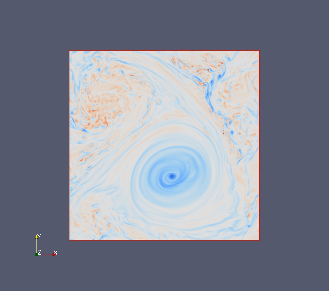
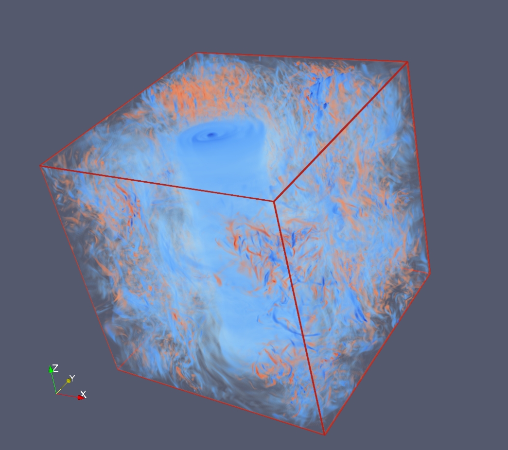
Figure 12: A visualization of the flow where the $z$-component of the vorticity is shown. The panel on the left shows the computational box viewed from the top, while the same flow is shown viewed from the side on the right panel where the opacity has been reduced so that the structures inside the computational box can be seen.

With this observation one can easily understand how saturation is reached in the large scales. The fast rotation leads to a quasi-two-dimensionalization of the system that leads to an inverse cascade of energy. As energy of the 2D3C part of the flow increases it reaches the largest scale of the system where it forms two counter rotating vortexes. As the amplitude of these two vortexes is increased a point is reached that the vertical vorticity of the counter rotating vortex will cancel the effect of rotation locally leading to an order one value of the local Rossby number. Then the quasi-2D constrain that leads to the inverse cascade and the pile-up of energy to the large scales is broken and energy starts to flow back to the small scales. Such a mechanism of course implies that saturation is reached when the eddy turn-over-time of the condensate is the same order with the rotation period or more simply $\mathrm{{Ro}}_{{}_{U}}\sim 1$. Indeed in figure 13 we plot $\mathrm{{Ro}}_{{}_{U}}$ from all the runs that showed a condensate behavior as a function of $\mathrm{{Ro}}_{{}_{F}}$ (left panel) and as a function of $\mathrm{{Re}}_{{}_{F}}$ (right panel)

Figure 13: $\mathrm{{Ro}}_{{}_{U}}$ as a function of $\mathrm{{Ro}}_{{}_{F}}$ (left panel) and $\mathrm{{Re}}_{{}_{F}}$ (right panel) for all the runs that lead to a quasi-2ED condensate. The $\mathrm{{Ro}}_{{}_{U}}=1$ behavior shown here can also be seen in the left panel of figure 2.

The value of $\mathrm{{Ro}}_{{}_{U}}$ appears to be independent of both $\mathrm{{Ro}}_{{}_{F}}$ and $\mathrm{{Re}}_{{}_{F}}$ thus the scaling $\mathrm{{Ro}}_{{}_{U}}\sim 1$ is verified. This result implies that this state in unlikely to be described by an $\mathrm{{Ro}}_{{}_{U}}\to 0$ expansion as the eddy turn-over time is the same order with the rotation period. It also implies that condensates saturate by reaching a state of marginal inverse cascade (Seshasayanan et al., 2014).

6 Large $\mathrm{{Re}}_{{}_{F}}$, small $\mathrm{{Ro}}_{{}_{F}}$ asymptotic behavior of turbulence

The results so far have shown that different behaviors are present for large $\mathrm{{Re}}_{{}_{F}}$ and small $\mathrm{{Ro}}_{{}_{F}}$ depending on the ordering of these parameters. It is thus also expected that the basic energy balance relations ) that link the the forcing amplitude and the velocity amplitude with the energy injection/dissipation rate) will differ for the different states of the system. Knowledge of the relation of these quantities allows to determine the map between the control parameter pairs $(\mathrm{{Ro}}_{{}_{F}},\mathrm{{Re}}_{{}_{F}})$, $(\mathrm{{Ro}}_{{}_{U}},\mathrm{{Re}}_{{}_{U}})$ and $(\mathrm{{Ro}}_{{}_{D}},\mathrm{{Re}}_{{}_{D}})$.

In non-rotating turbulence in the high $\mathrm{{Re}}_{{}_{F}}$ limit it is expected that the role of viscosity is unimportant in the large scales. With this assumption the relation between the forcing amplitude, the velocity fluctuations amplitude $U$ and the energy dissipation rate can be derived by dimensional analysis. It results in the following two relations:

$$U\propto C_{{}_{U}}^{{}^{T}},\qquad\epsilon\propto C_{{}_{D}}^{{}^{T}}U^{3}q,$$ (63)

where the proportionality coefficients $C_{{}_{U}}^{{}^{T}},C_{{}_{D}}^{{}^{T}}$ are order one numbers. (Here it is reminded to the reader that $U$ stands for the root mean square velocity non-dimentionalized by $\sqrt{F_{0}L}$. Thus the first part of equation 63 simply implies the dimensional velocity amplitude is proportional to $\sqrt{F_{0}L}$). In the other limit for which $\mathrm{{Re}}_{{}_{F}}$ is very small then the nonlinearity can be neglected and obtain the laminar scaling

$$U\propto C_{{}_{U}}^{{}^{L}}\mathrm{{Re}}_{{}_{F}}q^{-2},\qquad\epsilon\propto C_{{}_{U}}^{{}^{L}}\mathrm{{Re}}_{{}_{U}}^{-1}{U}^{3}q\propto\mathrm{{Re}}_{{}_{F}}^{-1}q^{-2}$$ (64)

by balancing the forcing with the viscous term. These scalings are expected to be valid for weakly rotating flows $\mathrm{{Ro}}_{{}_{F}}\gg 1$ where the effect of rotation can be neglected.

For $\mathrm{{Ro}}_{{}_{F}}\lesssim 1$ however the rotation can not be neglected and this makes the energy balance relations for the high $\mathrm{{Re}}_{{}_{F}}$ limit less straight forward. The increase in complexity stems from the fact that: first even if $\mathrm{{Re}}_{{}_{F}}$ is large we cannot conclude independence on the viscosity with out also specifying the value of $\mathrm{{Ro}}_{{}_{F}}$. This limitation exists because in general rotation diminishes the energy cascade thus for any value of $\mathrm{{Re}}_{{}_{U}}$ there would exist a value of $\mathrm{{Ro}}_{{}_{U}}$ small enough so that energy cascade flux is comparable to the dissipation. Second even if viscosity is neglected in the large $\mathrm{{Re}}_{{}_{F}}$ limit we are still left with on non-dimensional parameter the Rossby number, making the derivation of scaling laws by simple dimensional analysis to require further physically motivated arguments.

For the Taylor-Green flow we have already showed that the flow is guaranteed to be laminar when the relations 34,35 hold. Thus in this range the desired relations can be directly be obtained from the laminar solutions that for $\mathrm{{Ro}}_{{}_{F}}\ll 1\,\,\&\,\,\mathrm{{Re}}_{{}_{F}}\propto\mathrm{{Ro}}_{{}_{F}}^{-1}$ become:

$$U\simeq\sqrt{3}\mathrm{{Ro}}_{{}_{F}},\qquad\epsilon\simeq 3q^{2}U^{3}\mathrm{{Re}}_{{}_{U}}^{-1}\simeq 9q^{2}\mathrm{{Ro}}_{{}_{F}}^{2}/\mathrm{{Re}}_{{}_{F}}$$ (65)

For large $\mathrm{{Re}}_{{}_{F}}$ and fast rotation rate wave-turbulence arguments based on three wave-interactions (see chapter 3 of Nazarenko (2011)) suggest that energy cascade rate to the small scales will be decreased by a factor $\mathrm{{Ro}}_{{}_{U}}$. This reasoning leads to the relations

$$U\propto C_{{}_{U}}^{{}^{WT}}\mathrm{{Ro}}_{{}_{F}},\qquad\epsilon\propto C_{{}_{D}}^{{}^{WT}}\mathrm{{Ro}}_{{}_{U}}U^{3}q$$ (66)

will hold. The first relation comes from a balance of the Coriolis term in the Navier Stokes equation with the forcing while the second relation is a weak turbulence estimate that is derived assuming an ensemble of random traveling waves whose fast de-correlation time leads to the reduction in the energy cascade rate by a factor proportional to their inverse speed (here $\mathrm{{Ro}}_{{}_{F}}$). These arguments however assume uniform and isotropic forcing and do not take into account the formation of condensates. Thus are not necessarily expected to hold for a structured forcing like the Taylor-Green.

Figure 14: $U^{2}$ (left panel) and $\epsilon$ (right panel) as a function of $\mathrm{{Ro}}_{{}_{F}}$ for all runs. Same symbols,colors,sizes are used as in figure 1.

In figure 14 we plot the basic quantities $U^{2}$ (left panel) and $\epsilon$ (right panel). as a function of $\mathrm{{Ro}}_{{}_{F}}$. We remind the reader that the same symbols were used as in figure 1 thus large symbols imply larger $\mathrm{{Re}}_{{}_{F}}$ while dark (violet online) symbols imply small $\mathrm{{Ro}}_{{}_{F}}$. Clearly different phases in the flow follow different scaling laws. For large $\mathrm{{Ro}}_{{}_{F}}$ the effect of rotation is not felt and thus the turbulent scaling 63 is recovered with both $U^{2}$ and $\epsilon$ being independent from $\mathrm{{Ro}}_{{}_{F}}\geq 1$ and independent from $\mathrm{{Re}}_{{}_{F}}$ for sufficiently large $\mathrm{{Re}}_{{}_{F}}$. As $\mathrm{{Ro}}_{{}_{F}}$ is decreased different behaviors are observed. The laminar runs reproduce the relation 65 with a clear scaling $U^{2}\propto\mathrm{{Ro}}_{{}_{F}}^{2}$. Since most of the laminar states examined are close to the stability boundary $\mathrm{{Ro}}_{{}_{F}}\propto\mathrm{{Re}}_{{}_{F}}^{-1}$, the $\epsilon\propto\mathrm{{Ro}}_{{}_{F}}^{2}/\mathrm{{Re}}_{{}_{F}}$ scaling appears as $\epsilon\propto\mathrm{{Ro}}_{{}_{F}}^{3}$ This however provides only an upper limit for the dissipation of the laminar states. The quasi-2D condensate states result in the scaling $U^{2}\propto\mathrm{{Ro}}_{{}_{F}}^{-2}$ in accordance with the results shown in figure 13. Note also the discontinuous change in $U^{2}$ that is a direct result of the sub-critical behavior of the condensate modes. The energy dissipation rate for these runs decreases initially as $\mathrm{{Ro}}_{{}_{F}}$ is decreased but then it seems to saturate at the smallest values of $\mathrm{{Ro}}_{{}_{F}}$ attained. This however will need to be verified at smaller $\mathrm{{Ro}}_{{}_{F}}$. A similar behavior is also observed for the runs that displayed a bursting behavior. The scaling $U^{2}\propto\mathrm{{Ro}}_{{}_{F}}^{-2}$ and $\epsilon\propto\mathrm{{Ro}}_{{}_{F}}^{0}$ is also observed for these modes for some range of $\mathrm{{Ro}}_{{}_{F}}$. This behavior however transitions to a laminar behavior at even smaller $\mathrm{{Ro}}_{{}_{F}}$ propably because not large enough $\mathrm{{Re}}_{{}_{F}}$ has been reached for these runs.

Figure 15: $\epsilon L/U^{3}$ as a function of $\mathrm{{Re}}_{{}_{U}}$ (left panel) and $\mathrm{{Ro}}_{{}_{U}}$ (right panel) for all runs. Same symbols,colors,sizes are used as in figure 1.

This section is concluded by discussing the properties of the energy dissipation rate as a function of the more commonly used control parameters $\mathrm{{Re}}_{{}_{U}}$ and $\mathrm{{Ro}}_{{}_{U}}$. Figure 15 displays $\epsilon L/U^{3}$ as a function of $\mathrm{{Re}}_{{}_{U}}$ (left panel) and $\mathrm{{Ro}}_{{}_{U}}$ (right panel). The right panel serves mostly to demonstrate that although some of the data points are grouped together in the left panel they correspond to different processes as can be realised by the different values of $\mathrm{{Ro}}_{{}_{U}}$ they occupy in the parameter space. The ratio $\epsilon L/U^{3}$ for non-rotating turbulence based on eq.63 is expected to scale like $\mathrm{{Re}}_{{}_{U}}^{-1}$ for small values of $\mathrm{{Re}}_{{}_{U}}$ while an asymptotic value (independent of $\mathrm{{Re}}_{{}_{U}}$) is expected to be reached at large enough $\mathrm{{Re}}_{{}_{U}}$. Reaching this asymptotic value indicates that the systems has reached a turbulent state for which large scale properties do not depend on viscosity and energy injection is balanced only by the energy flux to the small scales due to the nonlinearity (Kaneda et al., 2003). Indeed such a state is reached for our weakly rotating runs for $\mathrm{{Re}}_{{}_{U}}\gtrsim 800$ and $\mathrm{{Ro}}_{{}_{F}}\geq 0.4$ (ie diammond runs). For the fast rotating runs however (including both bursts and condensates) such a state is not reached and the ratio $\epsilon L/U^{3}$ continues to decrease as $\mathrm{{Re}}_{{}_{U}}^{-1}$ even at $\mathrm{{Re}}_{{}_{U}}\sim 10^{4}$. For these states most of the energy (and vorticity) is concentrated in a few large scales modes and thus they have a laminar scaling. However, since the saturation amplitude at the large scale is viscosity independent but depends only on $\Omega$, it is expected that at even larger $\mathrm{{Re}}_{{}_{U}}$ the vorticity at small scales will grow enough so that despite the large energy concentration in the large scale modes, vorticity will be dominated by the small scales and not the large and a viscosity free scaling will be obtained. This can be explained best by looking at the 1D energy spectrum in the right panel of figure 11. As $\mathrm{{Re}}_{{}_{F}}$ is increased the amplitude of energy in the large scales will remain fixed (so that $\mathrm{{Ro}}_{{}_{U}}=1$) but the large wavenumber viscous cut-off $k_{c}$ will extend to larger wavenumbers. Since the spectrum is sufficiently flat (less flat than $k^{-3}$) at large $\mathrm{{Re}}_{{}_{F}}$ the dissipation ($\propto\mathrm{{Re}}_{{}_{F}}^{-1}\int k^{2}E_{{}_{1D}}dk$) will be dominated by the small scales provided $k_{c}$ is sufficiently large. Thus a viscosity independent scaling is expected to be obtained in the $\mathrm{{Re}}_{{}_{F}}\to\infty$ limit. This however would require resolutions not attainable in the present study.

7 Summary and conclusions

Perhaps the most intriguing result of the present work is the demonstration that a simple two parameter system like the one under study can display such richness and complexity of behavior. Depending on the location in the parameter space the system can display laminar behavior, intermittent bursts, quasi-2D condensate states, and weakly rotating turbulence. All these behaviors can be obtained in the $\mathrm{{Re}}_{{}_{F}}\to\infty$ limit provided the appropriate scaling of $\mathrm{{Ro}}_{{}_{F}}$ with $\mathrm{{Re}}_{{}_{F}}$ is considered.

For high rotation rates laminar solution can be found in terms of an asymptotic expansion. Up to the ordering $\mathrm{{Ro}}_{{}_{F}}\propto\mathrm{{Re}}_{{}_{F}}^{-1/3}$ the laminar solution has no zeroth order projection to the 2D3C-flows. For $\mathrm{{Ro}}_{{}_{F}}\propto\mathrm{{Re}}_{{}_{F}}^{-1/5}$ the flow has an order one projection to 2D3C-flows and for even larger values of $\mathrm{{Re}}_{{}_{F}}$ no laminar solution that can be captured by the expansion exists. The realizability of the laminar flows is determined by their stability properties.

When $\mathrm{{Re}}_{{}_{F}}$ is increased and the conditions for stability are violated the system transitions sub-critically to a time dependent flow that exhibits intermittent bursts. The unstable modes involved can be predicted by an asymptotic theory, that takes in to account exact resonances and is valid in the limit $\mathrm{{Ro}}_{{}_{F}}\to 0$. The existence of exact resonances at the first order of the expansion that can drive the system unstable implies that the linear instability boundary is along the $\mathrm{{Ro}}_{{}_{F}}\propto\mathrm{{Re}}_{{}_{F}}^{-1}$ line. These modes drive the system on the dynamical time scale to high levels of energy where the asymptotic expansion fails and the resonance conditions are violated. After the burst the remaining energy is concentrated in a 2D3C flow that condensates in the largest available scale and decays on the viscous time scale. These bursts can be described of a low dimensional dynamical system, and thus do not describe a truly turbulent state.

As $\mathrm{{Re}}_{{}_{F}}$ is increased with respect to $\mathrm{{Ro}}_{{}_{F}}^{-1}$ and a relation $\mathrm{{Ro}}_{{}_{F}}\leq c\mathrm{{Re}}_{{}_{F}}^{-\alpha}$ is satisfied the system transitions again subcritically to a quasi-2D condensate. This state represents the rotating turbulence regime for the Taylor-Green flow as it the one obtained in the limit $\mathrm{{Re}}_{{}_{F}}\to\infty$ for any value of $\mathrm{{Ro}}_{{}_{F}}\leq 0.4$. The flow at this state is composed of a quasi2D condensate of vertical vorticity at the large scales and only weakly anisotropic small scale turbulence. Saturation of the large scale condensate comes from reaching values of $\mathrm{{Ro}}_{{}_{U}}=1$ at which point the counter-rotating vortex from the pair of vortexes that formed becomes unstable and cascades the energy to the small scales. The value of the exponent $\alpha$ is either $1/3$ or $1/5$. If energy injection is achieved by the coupling of inertial waves at second order then $\alpha=1/3$. If not then at third order it has already been shown that the forcing alone is capable at injecting energy to the flow and $\alpha=1/5$. The numerical simulations give more support to the scaling $\mathrm{{Ro}}_{{}_{F}}^{-1}\propto\mathrm{{Re}}_{{}_{F}}^{1/3}$ without however being decisive. Finally, the energy dissipation rate has not reached the viscosity independent scaling in this regime due to the large amplitude of the condensates, but it is expected to be reached at higher values of $\mathrm{{Re}}_{{}_{F}}$.

From these results there are a few points that worth being pointed out. First of all the first order expansion fails to describe the evolution of the 2D3C part of the flow. The small $\mathrm{{Ro}}_{{}_{F}}$ expansion that predicts independence of the 2D3C part of the flow can not predict the increase of the 2D3C flow that was observed both during the intermittent bursts stage and during to the quasi-2D state. Thus to describe the flow higher terms in the expansion need to be kept.

It was also found that for any value of the parameters examined ($\mathrm{{Re}}_{{}_{F}},\mathrm{{Ro}}_{{}_{F}}$) a phase that could be described as weak wave turbulence was not met. Fast rotating flows were either dominated by condensates or intermittent bursts. Possibly this is the case because only the value $q=2$ was used. For larger values of $q$ both the number of exact resonances and quasi-resonances would increase and the system would come closer to a continuous Fourier space where the assumptions of the weak-wave-turbulence theory better hold. However, it is noted that fully turbulent flows displayed the formation of quasi-2D condensates that reduced all flows to $\mathrm{{Ro}}_{{}_{U}}=1$. Thus in the steady state there is no guaranty that the prerequisite condition for weak turbulence $\mathrm{{Ro}}_{{}_{U}}\ll 1$ will be met at the steady state for this choice of forcing and for $\mathrm{{Ro}}_{{}_{F}}\ll 1$ even at larger $q$.

This last point also raises an interesting aspect of systems with inverse cascade. In the absence of a large scale dissipative mechanisms, the need to saturate the inverse cascade drove the system to marginality of the inverse cascade by reaching in the present case $\mathrm{{Ro}}_{{}_{U}}=1$. At this state there is a very weak inverse energy transfer just sufficient to sustain the large scale flow against viscosity. Aspects of such marginal states of inverse cascades have been recently investigated in more simplified models (Seshasayanan et al., 2014).

A further point worth pointed out by the present work is that referring to the large-Reynolds-small-Rossby limit without specifically prescribing the limiting procedure is meaningless, since different behaviors can be obtained for different scaling of the Reynolds number with the Rossby number. Different ordering of $\mathrm{{Re}}_{{}_{F}}$ with $\mathrm{{Ro}}_{{}_{F}}$ leads to different behaviors and scalings. Also the velocity amplitude used in the definition of the Reynolds and Rossby number is more than just a conventional formality in rotating turbulence. Thus one needs to be precise on the definitions used and the limiting procedure considered. From the present results the $\mathrm{{Ro}}_{{}_{D}},\mathrm{{Re}}_{{}_{D}}$ were shown to best describe the level of turbulence with respect to the rotation rate and the viscosity.

Finally, it is pointed out the necessity of numerical studies to cover systematically the parameter space in order to draw any general conclusions.