High-gain weakly nonlinear flux-modulated Josephson parametric amplifier using a SQUID-array

Abstract

We have developed and measured a high-gain quantum-limited microwave parametric amplifier based on a superconducting lumped LC resonator with the inductor L including an array of 8 superconducting quantum interference devices (SQUIDs). This amplifier is parametrically pumped by modulating the flux threading the SQUIDs at twice the resonator frequency. Around 5 GHz, a maximum gain of 31 dB, a product amplitude-gain $\times$ bandwidth above 60 MHz, and a 1 dB compression point of -123 dBm at 20 dB gain are obtained in the non-degenerate mode of operation. Phase sensitive amplification-deamplification is also measured in the degenerate mode and yields a maximum gain of 37 dB. The compression point obtained is 18 dB above what would be obtained with a single SQUID of the same inductance, due to the smaller nonlinearity of the SQUID array.

Although superconducting parametric amplifiers based on Josephson junctions are known and understood for decades Barone ; Yurke and Buks , they have recently received an increased attention Lenhert because of their ability to measure single quantum objects and engineer quantum fluctuations of a microwave field. They are extensively used to readout superconducting quantum bits Devoret JPC ; ParamFluxQ ; quantum trajectories or mechanical resonators Teufel at or near the quantum limit, i.e with minimum back-action imposed by quantum mechanics for the given amount of information taken on the system. They permitted for instance the measurement of quantum trajectories quantum trajectories and the implementation of quantum feedback schemes Siddiqi Quantuum Feedback ; Reversing quantum trajectories . In the field of quantum microwaves, they are also used to squeeze quantum noise and produce itinerant squeezed states for encoding quantum information Squeezed noise Mallet ; Gross squeezing or demonstrating fundamental effects like the reduction of the radiative decay of an artificial atom Siddiqi atom relaxation in squeezed .

Compared to the noisier high electron mobility transistor (HEMT) based amplifiers, these Josephson parametric amplifiers (JPA) suffer from limited bandwidth and from gain saturation at extremely low input power. A strong effort is thus made to increase the bandwidth and to mitigate saturation of JPAs by varying their design and mode of operation siddiqi PRB ; highdynamc ; JohnMartinis ; wifi paramp . In all cases, parametric amplification of a signal at angular frequency $\omega_{S}$ occurs by transfer of energy from a pump at frequency $\omega_{P}$ to the signal and to a complementary idler frequency $\omega_{I}$. For amplifiers based on resonators, one distinguishes the case of intrinsically nonlinear resonators with bare frequency $\omega_{R}$ that are pumped at $\omega_{P}\simeq\omega_{S}\simeq\omega_{R}$ directly on their signal line, from the (possibly linear) resonators whose frequency $\omega_{R}$ is parametrically modulated with a pump tone at $\omega_{P}\simeq 2\omega_{S}\simeq 2\omega_{R}$ on a dedicated line separated from the signal port. In the first case the intrinsic nonlinearity of the resonator is usually obtained by implementing all or part of its inductance by Josephson junctions (or superconducting weak links). The pumping at $\omega_{P}$ at sufficiently high amplitude modulates this nonlinear inductance at $2\omega_{P}$, and is responsible for a 4-wave mixing such that $2\omega_{P}=\omega_{S}+\omega_{I}$. In the present work, we are interested in the second case Wilson parametric oscillator ; Paramp NEC , for which the nonlinearity is due to an externally imposed parametric modulation of the frequency and is responsible for a 3-wave mixing such that $\omega_{P}=\omega_{S}+\omega_{I}$. The interest of this 3 wave mixing is that no pump mode propagates along the input and output signal lines and can blind a detector or spoil a squeezed field, at a close frequency. In practice, the true parametric modulation is usually obtained by embedding in the resonator inductance one or several SQUIDs, the Josephson inductance of which is modulated by an ac magnetic flux. The nonlinearity of the resonator inherited from the SQUID(s) is in this case an unwanted feature, which leads to saturation of amplification, and should thus be kept low. So besides the advantage of getting rid of the pump along the signal lines, a truly parametrically pumped amplifier can also be made more robust against saturation by reducing its nonlinearity without having to pump it more strongly. In this work, we test this idea and demonstrate a weakly nonlinear JPA with high gain, made of a lumped LC resonator with the inductor $L$ terminated by a SQUID array. The manuscript first summarizes the theoretical description of such a JPA, then describes the device implemented and its characterization setup, and finally presents the experimental data and a comparison between measured and calculated gain, bandwidth, and saturation.

I Theoretical summary and design choices

The specificity of the JPA presented here (pure 3 wave-mixing with spurious nonlinearity) makes the standard classical description of parametric amplifiers Yurke and Buks not directly applicable to it. This is why a comprehensive theoretical summary is given here, based on the theoretical work Paramp Vitaly (note that a similar theoretical treatment can be found in Eichler-Wallraff ). The equivalent circuit of the JPA is shown in the bottom-right corner of Fig. 1b. For a DC flux bias $\Phi_{DC}$, a parametric modulation $\delta L_{A}\cos(\omega_{P}t)$ of its array inductance $L_{A}$, and a microwave input signal $V_{S}\cos(\omega_{S}t+\chi)$, the JPA equation of motion at the lowest nonlinear order in phase $\varphi=1/\varphi_{0}\int Vdt$ across the total inductance $L=L_{g}+L_{A}(\Phi_{DC})$ or the capacitance $C_{R}$ is

$$\varphi^{\prime\prime}+2\Gamma_{a}\varphi^{\prime}+\omega_{R}^{2}[1+a_{P}(\Phi_{AC})\cos(\omega_{P}t)]\varphi+\alpha_{1}\varphi^{3}=\varphi_{S}\cos(\omega_{S}t+\chi),$$ (1)

where $\varphi_{0}=\hbar/2e=\Phi_{0}/2\pi$ is the reduced flux quantum, $\omega_{R}=2\pi f_{R}=1/\sqrt{L(C_{R}+C_{c})}$ the frequency of the resonator, $\omega_{P}=2\pi f_{P}$ the pumping frequency, $\Gamma_{a}=\omega_{R}/2Q$ its amplitude decay rate, $a_{P}=\delta L_{A}(\Phi_{AC})/L$ the relative pumping amplitude, $\alpha_{1}=-\omega_{R}^{2}p^{3}/2N^{2}$ the Josephson nonlinearity coefficient with $N$ the number of SQUIDs and $p=L_{J}/L$ the so-called participation ratio of the total Josephson inductance $L_{J}$ to the total inductance $L$; $\varphi_{S}$ is the drive amplitude proportional to $V_{S}$. Taking into account the finite ratio $\beta$ of each SQUID loop inductance to the inductance $L_{J1}$ of a single junction, the SQUID array inductance is $L_{A}=NL_{J1}\beta/4+L_{J}$ with $L_{J}=NL_{J1}/\left\{2\left[\cos\left(x\right)+\beta/2\sin^{2}\left(x\right)\right]\right\}$ Agustin Squid inductance and $x=\pi\Phi/\Phi_{0}$.

Equation (1) contains the parametric nonlinearity $\cos(\omega_{P}t)\varphi$ and the intrinsic Josephson nonlinearity $\alpha_{1}\varphi^{3}$ mentioned in the introduction. We rewrite it in the frame rotating at $\omega_{P}/2$ using the slow complex internal amplitude $A(t)$ defined by $\varphi(t)=A(t)\sqrt{Z_{R}}\mathrm{\mathrm{e}^{-i\omega_{P}t/2}}+\mathrm{cc}$, as well as the constant complex amplitude $B_{S}$ of the input signal and the slow output amplitude $C(t)$ related to the input and output voltages $V_{in,out}$ by $V_{in}(t)=i\varphi_{0}\sqrt{Z_{0}\omega_{S}}B_{S}\mathrm{\mathrm{e}^{-i\omega_{S}t}}/2+\mathrm{cc}$ and $V_{out}(t)=i\varphi_{0}\sqrt{Z_{0}\omega_{S}}C(t)\mathrm{\mathrm{e}^{-i\omega_{S}t}}/2+\mathrm{cc}$. Here, $Z_{0}$ is the impedance of the line, $Z_{R}=\sqrt{L/(C_{R}+C_{c})}$ the characteristic impedance of the resonator, and $\mathrm{cc}$ stands for the complex conjugate of the previous term. Neglecting fast oscillating terms (rotating wave approximation), one obtains Paramp Vitaly

$$\begin{cases}iA^{\prime}+(i\Gamma_{a}+\delta+\alpha\left|A^{2}\right|)A+\epsilon A^{*}=\sqrt{2\Gamma_{a}}B_{S}\mathrm{\mathrm{e}^{-i\Delta t}}\\ C=-i\sqrt{2\Gamma_{a}}A+B_{S}\end{cases},$$ (2)

where $\delta=\omega_{P}/2-\omega_{R}$ is the pump to resonator detuning, $\Delta=\omega_{S}-\omega_{P}/2$ the signal to pump detuning, $\alpha=-p^{3}Z_{R}\omega_{R}/16N^{2}$ the new nonlinear coefficient, and $\epsilon=\omega_{R}a_{P}=2\omega_{R}\kappa\Phi_{AC}/\Phi_{0}$ the pumping strength with $\kappa\propto pQ$ the relative frequency change per flux quantum deduced from the slope of the modulation curve $\omega_{R}(\Phi_{DC})$.

Although the most general stationary solution of Eq. (2) is a sum $\sum_{k\in\mathbb{Z}}\mathrm{A_{k}e}^{-ik\Delta t}$ of all harmonics at frequencies $\omega_{P}/2+k\Delta$, only the signal $A_{S}=A_{1}$ and the idler $A_{I}=A_{-1}$ contributions happen to be non negligible at not too high pumping strength. In this case, they obey

$$\begin{cases}\left\{\left[\delta_{r}+\alpha_{r}\left(\left|A_{S}\right|^{2}+2\left|A_{I}\right|^{2}\right)\right]+\Delta_{r}+i\right\}A_{S}+\epsilon_{r}A_{I}^{*}=\sqrt{2/\Gamma_{a}}B_{S}\\ \left\{\left[\delta_{r}+\alpha_{r}\left(2\left|A_{S}\right|^{2}+\left|A_{I}\right|^{2}\right)\right]-\Delta_{r}+i\right\}A_{I}+\epsilon_{r}A_{S}^{*}=0\\ C_{S}=-i\sqrt{2\Gamma_{a}}A_{S}+B_{S}\\ C_{I}=-i\sqrt{2\Gamma_{a}}A_{I}\end{cases}$$ (3)

with $\delta_{r}=\delta/\Gamma_{a}$, $\Delta_{r}=\Delta/\Gamma_{a}$, $\alpha_{r}=\alpha/\Gamma_{a}=-p^{3}Z_{R}Q/8N^{2}$ and $\epsilon_{r}=\epsilon/\Gamma_{a}$ the dimensionless detunings, nonlinear coefficient, and pumping strength, respectively.

Our goal is to make the nonlinearity $\alpha_{r}$ as small as possible and benefit from the linear signal and idler complex gains given by system (3) when $\alpha_{r}=0$, i.e.

$$\begin{cases}G_{S}=\frac{C_{S}}{B_{S}}=\frac{\delta_{r}^{2}-\Delta_{r}^{2}-1-\epsilon_{r}^{2}-2i\delta_{r}}{\delta_{r}^{2}-\Delta_{r}^{2}+1-\epsilon_{r}^{2}-2i\Delta_{r}}\\ G_{I}=\frac{C_{I}}{B_{S}}=\frac{2i\epsilon_{r}}{\delta_{r}^{2}-\Delta_{r}^{2}+1-\epsilon_{r}^{2}+2i\Delta_{r}}\mathrm{e}^{i2\chi}\end{cases},$$ (4)

yielding the power gains

$$\left|G_{S}\right|^{2}=1+\left|G_{I}\right|^{2}=1+\frac{4\epsilon_{r}^{2}}{\left[1-\epsilon_{r}^{2}+\delta_{r}^{2}-\Delta_{r}^{2}\right]^{2}+4\Delta_{r}^{2}}.$$ (5)

In the degenerate case corresponding to $\Delta=0$, the signal power gain becomes phase $\chi$ dependent and is given by

$$\left|G_{S,deg}\right|^{2}(\chi)=1+4\epsilon_{r}\frac{2\left[\epsilon_{r}-\delta_{r}\cos(2\chi)\right]+(1+\epsilon_{r}^{2}-\delta_{r}^{2})\sin(2\chi)}{\left(1-\epsilon_{r}^{2}+\delta_{r}^{2}\right){}^{2}}.$$ (6)

Equations (4-6) are valid only below the onset of parametric oscillations, that is of pump-induced auto-oscillations at zero signal $B_{S}$ for $\epsilon_{r}>1+$$\delta_{r}^{2}$. For sufficiently large pumping strength $\epsilon_{r}>0.42$ the power gain $\left|G_{S}\right|^{2}$ is larger than 2 at small $\Delta_{r}$ and $\delta_{r}$, and a gain bandwidth $\Delta\omega=2\pi\Delta f$ at $-3\,\mathrm{dB}$ can be defined. For the optimal pumping frequency $\delta_{r}=0$ we find

$$\frac{\Delta\omega}{2\Gamma_{a}}=\sqrt{\left(1+\epsilon_{r}^{2}\right)\left(\frac{2\epsilon_{r}}{\sqrt{\epsilon_{r}^{4}-6\epsilon_{r}^{2}-1}}-1\right)},$$ (7)

which yields a gain bandwidth product

$$\left|G_{S}\right|\Delta\omega/2\Gamma_{a}\simeq 1$$ (8)

that is constant within 10% above $7\,\mathrm{dB}$ gain. Then, saturation can be evaluated approximately in an easy way by noticing that as the internal amplitudes of oscillation $A_{S}$ and $A_{I}$ increase with the pumping strength and gain, they tend to the same value when $\left|G_{S}\right|^{2}\simeq\left|G_{I}\right|^{2}\gg 1$ (see Eq. (5)). Consequently, the terms in $\alpha_{r}$ in the first two equations of system (3) also converge to close values and play the very same role as the pump to resonator detuning $\delta_{r}$, which is itself responsible for a gain drop given by Eq. (6). Equating $\alpha_{r}\left|A_{S}^{2}+2A_{I}^{2}\right|$ at $\delta_{r}=0$ to the value $\delta_{r,sat}=0.35\sqrt{1-\epsilon_{r}^{2}}$ that produces a $-1\,\mathrm{dB}$ drop of $\left|G_{S}\right|^{2}-1$, leads to the following equivalent values for $A_{S}$ and $B_{S}$ (so called $1\,\mathrm{dB}$ compression point):

$$\begin{cases}A_{S,sat}^{2}\simeq\frac{0.35}{\left|\alpha_{R}\right|}\frac{\sqrt{1-\epsilon_{r}^{2}}}{1+2\epsilon_{r}^{2}}\\ \frac{B_{S,sat}^{2}}{\Gamma_{a}}\simeq\frac{0.17}{\left|\alpha_{R}\right|}\frac{\left(1-\epsilon_{r}^{2}\right)^{5/2}}{1+2\epsilon_{r}^{2}}\end{cases}$$ (9)

In addition, saturation at large gain $\left|G_{S}\right|$ has to occur when the peak current $i$ in the junctions is still well below their critical current $i_{c}$. Since at $\delta_{r}\sim 0$, $i/i_{c}=(1+\epsilon_{r})\left|A_{S}\right|p\sqrt{Z_{r}}/N$, keeping $i/i_{c}<0.5$ yields the design rule

$$pQ>21/\sqrt{\left|G_{S,max}\right|+1},$$ (10)

which imposes a minimum $p$ for low $Q$ and wide bandwidth JPAs.

In this work, we choose to implement a tunable amplifier in the 5-6 GHz range with a quality factor $Q$ of order 100, which should have a product gain$\times$bandwidth of $\sim 50\,\mathrm{MHz}$ according to Eq. (8). To reduce the maximum microwave pumping power corresponding to $\epsilon_{r}=Qa_{P}/2=1$, i.e. to a modulation $a_{P}\sim 1\%$ of the total inductance, a high participation ratio $p\simeq 0.5$ is chosen. On the other hand, in order to keep the nonlinearity $\alpha_{r}$ weak and to increase the $1\,\mathrm{dB}$ compression point $B_{S,sat}$, the tunable inductance is implemented with $N=8$ SQUIDs. In this case, the saturation power is increased by $N^{2}$ or $18\,\mathrm{dB}$, compared to the case of a single SQUID with the same total Josephson inductance. Finally, as $Z_{r}$ plays only a minor role in the nonlinearity$\alpha_{r}$ (in comparison with $p^{3}$and $N^{-2}$), its value will be simply chosen at the best convenience for implementing the lumped element resonator.

II Sample and measurement setup

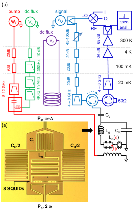
Figure 1: Experimental setup. (a) Optical micrograph of the tested parametric amplifier showing its $50\,\Omega$ coplanar waveguide (CPW) signal input port (top), its coupling capacitor $C_{c}$, its capacitor $C_{R}$ (left and right), its inductor $L_{g}$ (middle) terminated by an 8-SQUID arrays with total inductance $L_{A}\left(\Phi\right)$, and its split magnetic flux line coupled to a $50\,\Omega$ CPW (bottom). The DC current in the flux line sets the dc flux $\Phi_{DC}$ and the resonance frequency $f_{R}$ of the resonator, whereas the ac current parametrically pumps the resonator at $\omega_{P}\simeq 2\omega_{R}$. The black arrow points to the equivalent circuit. (b) Electrical circuit diagram showing (from left to right) the pump line, the dc flux line added to the pump with a bias tee, an additional flux line feeding a coil for compensating any flux offsets, the signal line, a circulator routing the reflected and amplified signal to a measurement line through an isolator protecting the sample from the noise of the first amplifier placed at 4 K. Feeding lines are attenuated and filtered. The output signal is split after amplification and analyzed both with a spectrum analyzer and by homodyne demodulation.

An optical micrograph of the JPA and its equivalent circuit are shown in Fig. 1a. This JPA is made of an interdigitated coplanar capacitor to ground (split in two parts) with capacitance $C_{R}=0.40\,\mathrm{pF}$ , in parallel with an inductance to ground $L$ combining in series a meander of inductance $L_{g}=0.80\,\mathrm{nH}$ with an array of 8 SQUIDs of total Josephson inductance$L_{J}=0.88\,\mathrm{nH}$ at zero magnetic flux $\Phi$. Being designed to be operated in reflection, this LC circuit is coupled to a single input-output signal line ($50\,\Omega$ coplanar waveguide - CPW ) through a $C_{c}=55\,\mathrm{fF}$ capacitance yielding a characteristic impedance $Z_{r}\backsimeq 65\,\Omega$ and a quality factor $Q\simeq 70$ at $\Phi=0$. On the other side of the device a $50\,\Omega$ CPW line shorted to ground by two loops coupled inductively to 4 SQUIDS each, serves both for their DC flux biasing and for parametric pumping. Note that after compensation of any global DC flux offset, the magnetic fluxes $\Phi$ are exactly opposite in the left and right 4 SQUID sub-arrays, which yields the same inductance modulation.

The device was fabricated on a thermally oxidized Si chip by sputtering $170\,\mathrm{nm}$ of niobium and patterning the whole structure (except the SQUID array) by optical lithography and $\mathrm{CF_{4}-Ar}$ reactive ion etching. The SQUID array was then fabricated by e-beam lithography and double-angle evaporation of aluminum with oxidation of the first Al layer. Each SQUID has a loop area of $8\,\mathrm{\mu m}\times 15\,\mathrm{\mu m}$ and two junctions with nominal area $2.2\,\mathrm{\mu m}\times 0.7\,\mathrm{\mu m}$ and tunnel resistance $141\,\Omega$, yielding $\beta\simeq 0.1$. The active antenna wires of the pump line are positioned $16\mathrm{\,\mu m}$ away from the SQUID centers.

The measurement set-up is schematized in Fig. 1b. A small superconducting coil is used to compensate the global DC flux offset. DC flux biasing and AC pumping of the SQUIDs are obtained by two attenuated and filtered lines combined with a bias-tee. The input line includes attenuators at various temperatures and a $4-8\,\mathrm{GHz}$ bandpass filter. The $-71.5\,\mathrm{dB}$ and $-51\,\mathrm{dB}$ transmissions of the input and pumping lines are calibrated with a $\pm 1\,\mathrm{dB}$ uncertainty. The reflected and amplified signal is routed to the output line by a cryogenic circulator with $-18\,\mathrm{dB}$ isolation. This output line includes an isolator for protecting the sample from higher temperature noise, a $4-8\,\mathrm{GHz}$ filter, a cryogenic high electron mobility transistor (HEMT) amplifier at 4K with $38\,\mathrm{dB}$ gain and a calibrated noise temperature of $3.8\,\mathrm{K}$, as well as additional room temperature amplifiers. The output signal is finally analyzed using a spectrum analyzer or a homodyne demodulator followed by a digitizer. Microwave generators for the input signal and pump are precisely phase locked.

III Experimental results

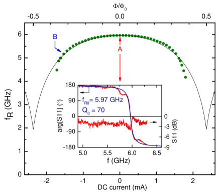
Figure 2: DC flux modulation. Experimental (dots) and calculated (line) resonator frequency $f_{R}$ as a function of the DC current in the on-chip flux line (see Fig.1a) measured by fitting the phase of a weak signal reflected on the resonator in absence of parametric pumping, as shown in the inset for zero flux bias (point A). We attribute the two shoulders on the sides of the measured resonance to multiple wave interferences due to an imperfect impedance matching somewhere in the setup. Parameters used for calculation of the modulation curve are $f_{R0}$, $p=0.45$, and $\beta=0.1$ . Full characterization in the next figures are done at working point B.

Measurements were performed in a dilution refrigerator at the temperature of $30-40\,\mathrm{mK}$. As a preliminary characterization, the resonance was measured with a vectorial network analyzer by recording the phase of the reflected signal at zero pumping and at a nominal input power $P_{S,n}=-126\,\mathrm{dBm}$ small enough to avoid any nonlinear effects (all nominal powers mentioned here and below refer to powers at the sample ports given the calibration of the lines). Inset of Fig. 2 shows this resonance at zero flux with a fit of the curve yielding a maximum frequency of $f_{R0}=5.97\,\mathrm{GHz}$. The comparison with the $f_{R1}=8.06\,\mathrm{GHz}$ resonance frequency of a similar resonator with shorted junctions yields $p=1-(f_{R0}/f_{R1})^{2}=0.45$, close to the $0.42$ design value. Fitting the expression $-2\arctan[2Q(f_{S}/f_{R}-1)]$ to the measured resonance curve also gives the quality factor $Q_{0}\simeq 70$, with however limited accuracy due to a setup imperfection yielding spurious multiple wave interferences (see shoulders in inset of Fig. 2). The main graph of Fig. 2 shows the variation of $f_{R}$ as a function of the applied flux $\Phi$ and its comparison with the theoretical prediction from section I. The agreement is only qualitative especially above $0.35\,\Phi_{0}$ where $f_{R}$ decreases faster than predicted by our simple model that does not include either the flux inhomogeneity in the different SQUIDs or the possible penetration of the flux through the junctions.

For characterizing amplification, the input and output lines are then connected as shown in Fig. 1. The signal and idler gains are measured with the spectrum analyzer by comparing the output powers of the signal and idler without and with parametric pumping at $f_{P}=2f_{R}$. The gains increase with $\left|\Phi_{DC}\right|$ and the slope of the modulation curve at fixed absolute pumping power. In the following measurement, signal amplification is fully characterized at the working point ($\Phi_{1}/\Phi_{0}=-0.32$, $f_{R1}=5.17\,\mathrm{GHz}$), i.e. point B on Fig. 2, where the slope $\kappa_{1}=1.62$ is at the same time large and in agreement with the predicted value. At this point the SQUID array model predicts a participation ratio $p_{1}=0.59$ and a quality factor $Q_{1}=81$.

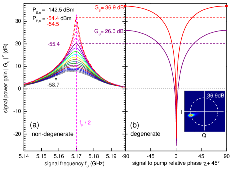
Figure 3: Signal power gain $\left|G_{S}\right|^{2}$ at working point B of Fig. 2 for a nominal input power $P_{S,n}=-142.5\,\mathrm{dBm}$. (left) Non-degenerate gain as a function of the signal frequency $f_{S}$ at different nominal pumping powers $P_{P,n}$ between $-58.7\,\mathrm{dBm}$ and $-54.4\,\mathrm{\mathrm{dB}m}$ (top dashed curve just before the onset of parametric oscillation in the absence of incident signal). (b) Phase sensitive degenerate gain for $P_{P,n}=-54.4\,\mathrm{dBm}$ and $-55.4\mathrm{\,dBm}$. (inset) Demodulated signal in the IQ plane at maximum gain ($P_{P,n}=-54.4\,\mathrm{dBm}$) filtered at 1 MHz. I and Q voltages are digitized at 1 MSample/s during 2 s, and the color encodes the density of samples from 0 (dark blue) to maximum (red).

The non-degenerate ($\Delta\neq 0$) signal power gain $\left|G_{S}\right|^{2}$ is measured with the pump frequency $f_{P}=2f_{R}$ ($\delta=0$) as a function of the signal frequency $f_{S}$ for increasing nominal pump power $P_{P,n}$, at an input power $P_{S,n}=-142.5\,\mathrm{dBm}$ sufficiently low to avoid the saturation at the highest gain. Close to the resonance, a minimum detuning $\delta/2\pi=5\,\mathrm{kHz}$ is used to avoid operation in the degenerate mode. Figure 3a shows the gain increase up to $31.8\,\mathrm{dB}$ (dashed top curve, for which parametric oscillations are about to start) and the corresponding bandwidth decrease. The maximum power gain $\left|G_{S}\right|^{2}$ and the corresponding $-3\,\mathrm{dB}$ bandwidth $\Delta f$ deduced from Fig. 3 are plotted on Fig. 4b together with the amplitude-gain $\times$ bandwidth product $\left|G_{S}\right|\Delta f$. This product happens to be almost constant around $61\,\mathrm{MHz}$ over the whole $7\,\mathrm{dB}-30\,\mathrm{dB}$ gain range. Besides, the idler gain (data not shown) approaches the signal gain at large values.

In order to check that the amplifier operates close to the quantum limit, i.e. with a noise temperature of order $T_{N}=hf_{R}/2k_{B}\simeq 125\,\mathrm{mK}$ noise review Clerk devoret , the variation of the signal and noise powers are compared when switching on and off the pump: from the $2.9\,\mathrm{dB}$ increase of the noise when switching on a $18.4\,\mathrm{dB}$ gain, from the calibrated $3.8\pm 0.3\,\mathrm{K}$ noise temperature of the HEMT amplifier alone in a separate run, and from the $1.7\pm 0.2\,\mathrm{dB}$ attenuation of elements placed below 250 mK between the sample and the HEMT amplifier, we deduce an apparent noise temperature of only $80\pm 10\,\mathrm{m\mathrm{K}}$. This value is smaller than the expected quantum limit of $125\,\mathrm{mK}$, a discrepancy that shows that modeling the line by a simple attenuator is not sufficient, as supported by our observation of the setup imperfection already mentioned. This result nevertheless indicates that our JPA is not far from the quantum limit. A more precise determination of $T_{N}$ would require a much more precise control and calibration of the low temperature part of the measurement line, as well as a switch to connect the detection chain either to the JPA or to a low temperature reference noise source Squeezed noise Mallet .

The phase dependent gain in the degenerate case ($\delta=0$ ) was then measured with $f_{S}=5.17\,\mathrm{GHz}$ by varying the phase $\chi$ of the signal with respect to the pump; it is shown on Fig. 3b for the two values of the pump power that correspond to a $20\,\mathrm{dB}$ gain and to the maximum gain in the non-degenerate mode. As expected the maximum degenerate gain is $6\,\mathrm{dB}$ larger than the non-degenerate gain at almost the same frequency. At the highest degenerate gain of $36.9\,\mathrm{dB}$, it was checked using the IQ demodulator (see inset of Fig. 3b) that the phase of the amplified signal is stable over minutes and that the output signal drops down to zero (no parametric oscillation) when the input signal is switched off. As the phase $\chi$ is varied, the measured degenerate gain varies as expected, the lowest value of $-25\,\mathrm{dB}$ resulting from the uncontrolled interference between the deamplified signal and the $\sim-18\,\mathrm{dB}$ leak of input signal through the circulator (see Fig. 1). This strong deamplification and the low noise temperature indicate that our JPA could also be used as a vacuum squeezer. In the inset of Fig. 3 the elongation of the Gaussian spot along the amplified quadrature shows that after parametric amplification the noise coming from the sample at $f_{S}=5.17\,\mathrm{GHz}$ overcomes the noise of the cryogenic amplifier placed at $4\,\mathrm{K}$, the size of which is given by the spot size in the perpendicular direction. In this latter direction we observe that the spot size is reduced by 1.1% when switching on the parametric pumping. This reduction is twice as small as the 2.2% expected from deamplification of vacuum noise, which is again related to the difficulty to determine the noise temperature of the whole setup.

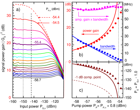
Figure 4: Amplifier characterization at the working point B of Fig. 2 for non-degenerate pumping. (a) Signal power gain as a function of the nominal input power $P_{S,n}$ showing the saturation at the same nominal pumping powers $P_{P,n}$ as in Fig. 3a (top dashed line corresponds again to the onset of parametric oscillation). Vertical dashed and dotted line correspond to the input powers where gain was measured in Fig. 3 and where reference gain for saturation was defined, respectively. (b) Power gain $\left|G_{S}\right|^{2}$, bandwidth $BW$, and product $\left|G_{S}\right|\times BW$ deduced from measurements (dots) of Fig. 3a at $P_{S,n}=-142.0\,\mathrm{dBm}$, and calculated (solid lines) from the model with the parameters indicated in the text. (c) 1 dB compression point deduced from (a) (dots), calculated from the model (solid line), and calculated with the sames parameters but only one SQUID (dashed line). Note that given the $\pm 1\,\mathrm{dB}$ precision on the calibration of the pumping and signal lines, $+0.8\,\mathrm{dB}$ and $-1.0\,\mathrm{dB}$ were added to the nominal $P_{P,n}$ and $P_{S,n}$ values to match the data to the theoretical curves at low pumping strength. The vertical dotted line indicates the frontier between parametric amplification and parametric oscillation (infinite gain) for the linear model.

Finally, the saturation of the JPA is measured by recording the non-degenerate signal power gain as a function of the signal input power $P_{S,n}$ for the same series of pump powers $P_{P,n}$ as before (see Fig. 4a). The signal gain is almost constant at low input power and then decreases above a $P_{P,n}$ dependent threshold in $P_{S,n}$ (however with a small bump of up to $1\,\mathrm{dB}$ just before saturation possibly due to higher orders in non-linearity). In practice, the $1\,\mathrm{dB}$ compression point is defined as the input power $P_{S,sat}$ at which the gain is $1\,\mathrm{dB}$ lower than at $P_{S,n}=-150\mathrm{\,dBm}$; it is plotted on Fig. 4c. The set of measurements of Figs. 4b-c is then compared to the linear model of section I: the power gain, bandwidth, product amplitude-gain $\times$ bandwidth, as well as the $1\,\mathrm{dB}$ compression point of Eqs. (6-9) are calculated by using the values of $f_{R1}$, $p_{1}$, $\kappa_{1}$ and $Q_{1}$ indicated above and are plotted on Fig. 4. Given the $\pm 1\,\mathrm{dB}$ uncertainty on the calibration of the signal and pump lines, the nominal input and pump powers were shifted by $+0.8\,\mathrm{dB}$ and $-1.0\,\mathrm{dB}$ to match the theory at the lowest pumping power. The agreement between the overall measured data and the model is surprisingly good given the crudeness of the linear model. This fair agreement validates the idea of increasing the number $N$ of SQUIDs to increase the saturation power that scales with $N^{2}$. With a single SQUID having the same total inductance as the array implemented here (about $1.7\,\mathrm{nH}$), the saturation would have been $N^{2}=18\,\mathrm{dB}$ lower, as indicated by the dashed line of Fig. 4c. The discrepancy between experimental data and the model increases with $P_{p}$ as the nonlinearity plays a more important role, and the actual parametric amplification region extends a bit over the theoretical parametric oscillation region of the linear model (dotted line of Fig. 4).

The performances of the present device are comparable to those of other truly parametric amplifiers recently made. Due to our choice of a rather large $Q\thicksim 70$, the gain bandwidth product is smaller than what was obtained for instance in Hartridge-Siddiqi with $Q\thicksim 10$. In JohnMartinis , the direct coupling of the resonator to a cleverly engineered frequency dependent external impedance yielded an even lower Q and a bandwidth above 500 MHz. Despite the use of $N=8$ SQUIDs, the 1dB compression point obtained here is not very high due to its scaling as $N^{2}Q^{-2}p^{-3}$ and to the large participation ratio and quality factors chosen to minimize the pump power: it is however about 12 dB above a similar amplifier made of a single SQUID with about the same critical current Paramp NEC and only a few dB below another one Hartridge-Siddiqi with smaller participation ratio $p$ (three times larger critical current Ic) and Q.

In terms of perspectives, equations (8-10) predict that with a similar geometry N$\sim 10$, a smaller $Q\sim 10$, and higher critical currents yielding $p\sim 0.25$, a bandwidth of $\sim 50\,\mathrm{MHz}$, and a compression point $\sim-100\,\mathrm{dBm}$ should be obtained at $20\,\mathrm{dB}$ gain. This would require a larger pump power, i.e. a larger flux modulation $\Phi_{AC}\varpropto 1/pQ$ at constant gain, which would reach $0.1\Phi_{0}$. Such a large modulation could be technically difficult to achieve. Increasing the number of SQUIDs is also an obvious optimization axis: If theoretically the array length has just to be kept much smaller than the pump wavelength so that all SQUIDS are pumped in phase, the practical difficulty is to DC flux bias and homogeneously modulate all the SQUIDs.

In summary, a lumped element truly parametric Josephson amplifier has been designed and characterized. Its inductance is implemented by a SQUID array to limit its nonlinearity and increase the maximum allowed input power. With a quality factor of 70 - 80, this simple device provides a gain of up to $30\,\mathrm{dB}$, a product amplitude-gain$\times$bandwidth of $61\,\mathrm{MHz}$, and a $1\,\mathrm{dB}$ compression point of $-123\,\mathrm{dBm}$ at $20\,\mathrm{dB}$ gain. Although its behavior is in agreement with theory and demonstrates the advantage of using a SQUID array, it can still be optimized by reducing both its quality factor and its Josephson participation ratio to the inductance and/or by increasing the number of SQUIDs in the array. Operated close to the quantum limit, this truly parametric amplifier could also be used as a quiet and strong squeezer in degenerate mode or as the first stage of amplification in a superconducting quantum bit readout.

References

- (1) A. Barone and G. Paterno, Physics and applications of the Josephson effect (Wiley, New York, 1982), chap. 11.
- (2) B. Yurke, L. R. Corruccini, P. G. Kaminsky, L. W. Rupp, A. D. Smith, A. H. Silver, R. W. Simon, and E. A. Whittaker, Phys. Rev. A 39, 2519 (1989).
- (3) M. A. Castellanos-Beltran and K. W. Lehnert, Appl. Phys. Lett. 91, 083509 (2007).
- (4) K. W. Murch, S. J. Weber, C. Macklin, and I. Siddiqi, Nature 502, 211–214 (2013).
- (5) R. Vijay, C. Macklin, D. H. Slichter, S. J. Weber, K. W. Murch, R. Naik, A. N. Korotkov, and I. Siddiqi, Nature 490, 77-80 (2012) .
- (6) B. Abdo, F. Schackert, M. Hatridge, C. Rigetti, and M. Devoret, Appl. Phys. Lett. 99, 162506 (2011).
- (7) Z. R. Lin, K. Inomata1, W. D. Oliver, K. Koshino, Y. Nakamura, J. S. Tsai, and T. Yamamoto, Appl. Phys. Lett. 103, 132602 (2013).
- (8) J. D. Teufel, T. Donner, Dale Li, J. W. Harlow, M. S. Allman, K. Cicak, A. J. Sirois, J. D. Whittaker, K. W. Lehnert, and R. W. Simmonds, Nature 475, 359–363 (2011).
- (9) G. de Lange, D. Ristè, M. J. Tiggelman, C. Eichler, L. Tornberg, G. Johansson, A. Wallraff, R. N. Schouten, and L. DiCarlo , Phys. Rev. Lett. 112, 080501 (2014).
- (10) F. Mallet, M. A. Castellanos-Beltran, H. S. Ku, S. Glancy, E. Knill,3 K. D. Irwin, G. C. Hilton, L. R. Vale, and K.W. Lehnert, Phys. Rev. Lett. 106, 220502 (2011).
- (11) E. P. Menzell, R. Di Candia, F. Deppel, P. Eder, L. Zhong, M. Ihmig, M. Haeberlein, A. Baust, E. Hoffmannl, D. Ballester, K. Inomata, T. Yamamoto, Y. Nakamura, E. Solano, A. Marx, and R. Gross, Phys. Rev. Lett. 109, 250502 (2012).
- (12) K. W. Murch, S. J. Weber, K. M. Beck, E. Ginossar, and I. Siddiqi. Nature 499, 62 (2013).
- (13) O. Yaakobi, L. Friedland, C. Macklin, and I. Siddiqi. Phys. Rev. B 87, 144301 (2013).
- (14) B. H. Eom, P. K. Day, H. G. LeDuc and J. Zmuidzinas, Nature Phys. 8, 623 (2012).
- (15) Josh Mutus, Ted White, Rami Barends, Yu Chen, Zijun Chen, Ben Chiaro, Andrew Dunsworth, Evan Jeffrey, Julian Kelly, Anthony Megrant, Charles Neill, Peter O’Malley, Pedram Roushan, Daniel Sank, Amit Vainsencher, James Wenner, Kyle Sundqvist, Andrew Cleland, and John Martinis, arXiv:1401.3799.
- (16) A. Narla, K.M. Sliwa, M. Hatridge, S. Shankar, L. Frunzio, R. J. Schoelkopf, M.H. Devoret, arXiv:1404.4979v1 (2014).
- (17) C. M. Wilson, T. Duty, M. Sandberg, F. Persson, V. Shumeiko, and P. Delsing, Phys. Rev. Lett. 105, 233907 (2012).
- (18) T. Yamamoto, K. Inomata, M. Watanabe, K. Matsuba, T. Miyazaki, W. D. Oliver, Y. Nakamura, and J. S. Tsai, Appl. Phys. Lett. 93, 042510 (2008).
- (19) C. Eichler and A. Wallraff, EPJ Quantum Technology (2014).
- (20) A. Palacios-Laloy, PhD thesis p.187, UPMC (2010).
- (21) W. Wustmann and V. Shumeiko, Phys. Rev. B 87, 184501 (2013).
- (22) A. A. Clerk, S. M. Girvin, Florian Marquardt, and R. J. Schoelkopf, Rev. Mod. Phys. 82, (2010).
- (23) M. Hatridge, R. Vijay, D. H. Slichter, John Clarke, and I. Siddiqi, Phys. Rev. B 83, 134501, (2011).