Spectral and Timing Analysis of the

Prompt Emission of Gamma Ray Bursts

A Thesis

Submitted to the

Tata Institute of Fundamental Research, Mumbai

for the degree of Doctor of Philosophy

in Physics

by

Rupal Basak

School of Natural Sciences

Tata Institute of Fundamental Research

Mumbai

Final Submission: Aug, 2014

To my Parents

Chapter 0 List of Publication

Publications in Refereed Journals

1. “Time-resolved Spectral Study of Fermi GRBs Having Single Pulses”, Basak, R. & Rao, A. R. (2014), MNRAS, 442, 419

2. “Time Resolved Spectral Analysis of the Prompt Emission of Long Gamma ray Bursts with GeV Emission”, Rao, A. R., Basak, R., Bhattacharya, J., Chanda, S., Maheshwari, N., Choudhury, M., Misra, R. (2014), RAA, 14, 35

3. “Pulse-wise Amati Correlation in Fermi Gamma-ray Bursts”, Basak, R. & Rao, A. R. (2013a), MNRAS 436, 3082

4. “A Lingering Non-thermal Component in the Gamma-ray Burst Prompt Emission: Predicting GeV Emission from the MeV Emission”, Basak, R. & Rao, A. R. (2013b), ApJ 775, 31

5. “A New Method of Pulse-wise Spectral Analysis of Gamma Ray Bursts”, Basak, R. & Rao, A. R. (2013c), ApJ 768, 187

6. “Correlation Between the Isotropic Energy and the Peak Energy at Zero Fluence for the Individual Pulses of Gamma-Ray Bursts: Toward a Universal Physical Correlation for the Prompt Emission”, Basak, R. & Rao, A. R. (2012a), ApJ 749, 132

7. “Measuring the Pulse of GRB 090618: A Simultaneous Spectral and Timing Analysis of the Prompt Emission”, Basak, R. & Rao, A. R. (2012b), ApJ 745, 76

Publications in Conference Proceedings

1. “GRB as luminosity indicator”, Basak, R. & Rao, A. R. (2014), Proceedings of IAU Vol 9, symposium No. 296, pp 356-357

2. “A new pulse-wise correlation of GRB prompt emission: a possible cosmological probe”, Basak, R. & Rao, A. R. (2013b), 39th COSPAR Scientific Assembly, Mysore, India, 2012cosp, 39, 106.

3. “Pulse spectral evolution of GRBs: implication as standard candle”, Basak, R. & Rao, A. R. (2013b) Gamma-Ray Bursts 2012, Munich, Germany, PoS (GRB 2012) [081]

Chapter 1 GRBs: The Extreme Transients

“… probably hotter, more violent, but what are they? .. We are aware of something we call a hypernova … we got supernova. Bigger, better — hypernova … these flashes are the brightest things in the gamma-ray sky …”

— Prof. Jocelyn Bell Burnell

(“Star glitter - the story of gold”, Public lecture, TIFR, January 16, 2014)

1 Overview

Gamma-ray Bursts (GRBs) are fascinating astrophysical objects in many aspects. They are believed to be catastrophic events marking the formation of compact objects, most probably stellar mass blackholes (BHs). A class of GRBs are associated with the explosive death of a very special kind of massive star (“collapsar”; Woosley 1993, or “hypernova”; Iwamoto et al. 1998), while another class is suggested to occur via merging of two compact objects, such as a binary neutron star (NS), or a NS and a BH. Frequently attributed with superlatives, GRBs are truly the most extreme transient phenomenon:

• (i) They are the most efficient astrophysical power house known to mankind (typical luminosity, $L_{\rm GRB}\sim 10^{52}~{}\rm erg~{}s^{-1}$). Their luminosity is many times higher than supernovae, which release the same amount of energy over a much longer period.

• (ii) More remarkably, most of this energy is released during a very brief episode (a few milliseconds to hundreds of seconds in observer frame), termed as the prompt emission phase. During this brief period a GRB radiates mostly in the form of $\gamma$-rays — a few keV to tens of MeV, and its intensity outshines all other $\gamma$-ray objects combined. The burst proper is followed by a longer lasting afterglow phase (observed over a few tens of days to months) in longer wavelengths ranging from x-rays to optical and radio. Even during the first day of x-ray and optical afterglow a GRB is about ten thousand times brighter than the brightest quasars, which in turn are hundred to thousand times brighter than their underlying galaxies.

• (iii) Due to the high luminosity a GRB is visible over a very large distance, corresponding to a very early epoch in cosmic history. The highest known redshift ($z$) is 9.4 (Cucchiara et al. 2011) which corresponds to only $\sim$ 5% of the present age of the universe. For this reason, GRBs are suggested as the best possible high-$z$ luminosity indicators.

• (iv) GRBs achieve their high luminosity by means of relativistic bulk motion with a Lorentz factor ($\Gamma$) reaching $\sim 100-1000$. The second most relativistic objects are BL Lacertae with $\Gamma\sim 10-20$, maximally $\Gamma\sim 50$ (Lister et al. 2009).

There are two broad aspects of GRB research — a. understanding the event itself, and b. using GRBs as tools e.g., studying cosmic star formation history, and using GRBs as luminosity indicators at high $z$. The prompt and afterglow phase are the most important observables for understanding the physics of GRBs, while $z$ measurement, chemical study of the burst environment etc. are essential for using GRBs as tools. During the prompt emission, a GRB generally has a rapid time variability, while the afterglow has a smooth time profile (see Section 1.4 for details). It is generally believed that the prompt emission of a GRB has an “internal” origin, and the time variability directly reflects the activity of the central object. The afterglow phase is more or less related to the “external” circumburst medium (Section 1.5). The afterglow phase is well studied and the data generally shows excellent agreement with a standard model, known as the “fireball shock” model (e.g., Mészáros & Rees 1997, Reichart 1997, Waxman 1997, Vietri 1997, Tavani 1997, Wijers et al. 1997). It is the prompt emission phase which remains a puzzle. There is no scarcity in the number of working models (e.g., Meszaros et al. 1994, Rees & Meszaros 1994, Thompson 1994, Daigne & Mochkovitch 1998, Pilla & Loeb 1998, Medvedev & Loeb 1999, Piran 1999, Lloyd & Petrosian 2000, Ghisellini et al. 2000, Panaitescu & Mészáros 2000, Spruit et al. 2001, Zhang & Mészáros 2002, Pe’er & Waxman 2004a, Ryde 2004, 2005, Rees & Mészáros 2005, Pe’er et al. 2005, 2006), but the unavoidable poor spectral quality of the $\gamma$-ray detectors challenges the correct identification of the fundamental model. As GRBs are very brief, single episode events coming from unpredictable directions of the sky, the detectors must have large field of view (and in many cases all-sky) to detect them. This severely affects the spectral quality as well as source localization. With the advent of Swift (Gehrels et al. 2004) and Fermi (Meegan et al. 2009) satellites, launched in 2004 and 2008 respectively, GRB research has entered a new era. The Swift has enabled many order better and quicker localization leading to $z$ measurement. The Fermi acquires data in a wide band, with good time resolution. With the current good quality data and large set of GRBs with known $z$, it is high time for extensive study of the prompt emission, identification of the underlying physics, and study GRBs as luminosity indicators. The aims of this thesis are (i) developing the most judicial way(s) for using the valuable data to describe the prompt emission, (ii) using prompt emission properties in favour of GRBs as luminosity indicators, (iii) developing a method to compare the spectral models of the prompt emission, and (iv) predicting interesting behaviours of the prompt and early afterglow phase.

2 Thesis Organization

The organization of the thesis is as follows. In this chapter, we shall briefly discuss the history and classification scheme, various observables e.g., lightcurve and spectrum, and the working model of GRBs. The next chapter (chapter 2) deals with the current instruments used for GRB prompt emission analysis. We shall focus on the Swift and the Fermi, the two main workhorses of modern GRB research. We shall point out the essential features of the satellites and detectors which make them superior compared to the other GRB experiments. The data analysis technique of these detectors will be described, and the issues with the joint Swift-Fermi fitting will be discussed. The prompt emission data provided by these satellites have very good spectral and timing resolution. However, it is important to use these information simultaneously in order to fully utilize the data. Hence, we need a new technique that judiciously describes the flux of a GRB as a simultaneous function of time and energy. The third chapter is entirely devoted for the new technique, which is developed using the existing empirical models in the literature. We shall see its versatile applications e.g., in deriving certain properties of GRBs, and studying GRBs as luminosity indicators. For these analyses, we shall choose all Fermi GRBs with known redshift (a total of 19 after sample selection). It is worthwhile to mention that though this model is very promising, the fact that it is based on empirical functions puts a limitation on its applicability. Hence, in the next chapters (fourth, and fifth), we shall discuss various alternative prompt emission models. These alternative models are applied on 5 bright GRBs, and 9 GRBs with single pulses. In order to test the merits of these different models, a new technique is developed. The analyses show that one of the alternative models is indeed a better description of the prompt emission. In Chapter 6, we will see some important predictive powers of this model. We shall choose 17 GRBs with very high energy photons to predict the high energy features. In chapter 7, we shall summarize the results, draw conclusions and describe the future extension of the work presented here.

3 History And Classification

1 Discovery, Afterglow and Distance Scale

The history of GRB research is full of observational and intellectual struggle, development of new techniques, exciting turnovers, and outstanding discoveries. Possibly the most important among these is the unambiguous discovery of the distance scale, which alone took nearly 30 years. In this section, we shall mention some brief historical facts, and refer the reader to the book by Katz (2002) for this exciting story. We shall also briefly discuss the classification scheme which is important in order to understand the progenitor of GRBs.

The GRB research began with the serendipitous discovery by Vela satellites on July 2, 1967 (Klebesadel et al. 1973; the burst is named as GRB 670702 following YYMMDD format). These satellites were launched by the U.S. Department of Defence to monitor nuclear explosions forbidden by the Nuclear Test Ban Treaty. With widely separated four independent satellites, Vela team discovered 16 bursts during 1969-1972, with duration of less than 0.1 s to $\sim 30$s, and time-integrated flux $\approx 10^{-5}$-$\sim 2\times 10^{-4}$ erg cm^-2 in 0.2-1.5 MeV band (Klebesadel et al. 1973). From the pulse arrival delay in different satellites, the approximate direction could be found, which excluded earth and sun as the possible source. As for distance of the sources, only lower limits (several earth-moon distance) could be put from the delay analysis.

For the next 25 years, several bursts were detected without any clue of their distance. The main obstacles for the distance measurement were poor localization of the $\gamma$-ray detectors (a few degree radius), and too brief a duration to look for the signature in other wavelengths. For a long time the distance remained highly debated even to the extent of whether the sources are Galactic or extra-galactic. By this time, Inter-Planetary Network (IPN; e.g., Cline & Desai 1976) provided a few to hundreds of sq. arcmin localization using several widely spaced spacecraft, but unfortunately with a considerable delay (days to months). Hence, no counterpart could be found.

The failure of direct localization triggered the use of statistical methods to infer the distance. If a large set of GRBs can be detected with a few degree of position accuracy, it is good enough to put the sources in the galactic coordinate. If the sources are extra-galactic, they should have an isotropic distribution. Various statistical tests are available to test the anisotropy e.g., dipole and quadrupole of the distribution (Hartmann & Epstein 1989; Briggs 1995). For perfect isotropic distribution and isotropic sampling, $\langle$cos $\theta\rangle$=0 and $\langle$sin${}^{2}\beta\rangle$=1/3, where $\theta$ is the angle between the direction of the burst and the Galactic centre, and $\beta$ is the Galactic latitude. Hartmann & Epstein (1989), using 88 IPN GRBs, showed that the bursts are isotropic within the statistical limits (also see Mazets & Golenetskii 1981). Another information comes from the tests of the uniformity of space distribution of the bursts e.g., log$N$/log$S$ test (Usov & Chibisov 1975, Fishman 1979), $V/V_{\rm max}$ test (Schmidt et al. 1988). Here, $N$ is the cumulative number of bursts with flux greater than $S$, and $V$ is the volume contained within the burst’s radial distance. The first test would give a constant slope of -3/2 if the bursts have uniform distribution on the Euclidean space. A different slope is expected for fainter bursts if the sources have cosmological distance. The $V/V_{\rm max}$ test takes the ratio of the actual (unknown) volume and the maximum allowed volume in which the burst could have been detected. In doing this it cancels the actual distance and depends only on the ratio of the peak ($C_{\rm p}$) and limiting ($C_{\rm lim}$) flux: $V/V_{\rm max}=(C_{\rm p}/C_{\rm lim})^{-3/2}$. For a uniform space distribution $\langle V/V_{\rm max}\rangle=1/2$. The $V/V_{\rm max}$ test is preferred over the log$N$/log$S$ test as it is independent of instrumental sensitivity. For a limited number of bursts from various experiments, deviations were reported from $\langle V/V_{\rm max}\rangle=1/2$ (Ogasaka et al. 1991: $0.35\pm 0.035$; Higdon et al. 1992: $0.400\pm 0.025$). A Galactic model could not reconcile the apparent isotropy and the inhomogeneity of the source distribution. However, a large group of researchers generally disbelieved the inferences drawn from a limited number of sources.

The sample size was not the only reason to generally disbelieve the extra-galactic origin, and stick to the Galactic model. A few attempts to calculate the prompt emission characteristics assuming a cosmological distance could not match observations (see Section 1.5). Moreover, a few earlier discoveries during late 1970’s and early 1980’s were already pointing towards a nearby origin. By this time, several models of GRBs were proposed (more than 100; Ruderman 1975; see Nemiroff 1994 for a later review), some of which were related to NSs. The Galactic NS model had strong observational evidences — (i) The burst of March 5, 1979 (Mazets et al. 1979) could be associated with a supernova remnant (SNR) of the nearby Large Magellanic Cloud (LMC). This burst had a steep spectrum, and a lightcurve with a strong initial $\sim 120$ millisecond pulse followed by very soft pulses. Though the spectrum and lightcurve of this burst was quite unusual for a GRB, it was generally attributed towards the diversity of GRBs. However, due to the detection of 16 more burst from the same source, it was later classified as a soft gamma repeater (SGR) coming from a highly magnetized neutron star (magnetar; e.g., Kouveliotou et al. 1987, Laros et al. 1987). Several other such sources were found later (Kouveliotou et al. 1992, Paczynski 1992; see Harding 2001 for a review). SNRs are known to harbour NSs, and the comparatively nearby distance of the burst made the Galactic NS origin plausible. (ii) In a few cases, cyclotron lines were reported (e.g., Murakami et al. 1988, Fenimore et al. 1988; also see Mazets et al. 1980), which corresponded to $\sim$ a few $\times 10^{12}$ G, typical for a NS. (iii) Finally, in order to account for the isotropy, the “nearby origin” could be pushed to the extended Galactic halo. In fact, extended halo origin was strongly supported by the discovery of high transverse velocity of neutron stars (NSs) which could populate the extended halo (Frail et al. 1994; cf. Bloom et al. 1999). If GRBs are indeed related to NSs, their isotropic distribution supports both the extended halo origin and the NS progenitor. The cosmological origin was supported only by Usov & Chibisov (1975), and later by Goodman (1986), and Paczynski (1986), based on the isotropic source distribution.

In the year 1991, NASA launched Compton Gamma Ray Observatory (CGRO), which along with three other instruments, carried specialized GRB instrument — Burst And Transient Source Experiment (BATSE; Fishman & Meegan 1995). The BATSE was designed to detect as many burst as possible, and thereby to rule out statistical bias from the inferences. It contained 8 NaI (Tl) scintillation detector modules in different directions. Each module consisted of one spectroscopic detector (SD), and one large area detector (LAD). The SD was sensitive in 20 keV-10 MeV band (with maximum effective area 126 cm²), while the LAD gave a very high effective area (maximum 2025 cm²) in a narrower band (20 keV-2 MeV). All the detectors were surrounded by plastic scintillators in active anti-coincidence to reduce the cosmic ray background. The BATSE had essentially an all-sky viewing so that the GRBs occurring at unpredictable directions could be located with some coarse position accuracy. The burst localization was done by comparing relative flux in the modules, and lay in the range 4^∘-10^∘. Though this is not an impressive accuracy, the success of the BATSE lies in the huge number of bursts detected over its lifetime (1991-2000). The final catalogue contained over 2500 bursts. For the first 1005 BATSE GRBs $\langle$cos $\theta\rangle=0.017\pm 0.018$, and $\langle$sin${}^{2}\beta-1/3\rangle=-0.003\pm 0.009$, which are respectively only $0.9\sigma$ and $0.3\sigma$ away from perfect isotropy (Briggs 1995). For 520 bursts $\langle V/V_{\rm max}\rangle=0.32\pm 0.01$ (Meegan et al. 1994) which confirmed the inhomogeneity. With the BATSE results the evidence of cosmological distance became stronger. However, the extended Galactic halo origin remained an option (Li & Dermer 1992). The lower limit on the size of the halo ($>20$ kpc) can be obtained by the requirement of the observed isotropy. With strong evidences in both sides, the famous “great debate” (Lamb 1995, Paczynski 1995) on whether the sources have extended Galactic halo or a cosmological origin, led to no final consensus.

The direct distance measurement was crucial, but it seemed difficult solely from $\gamma$-ray observation, unless by some lucky chance like the burst of March 5, 1979 (which was found in a SNR). The breakthrough came with the launch of Italian-Dutch satellite — Beppo-SAX (Boella et al. 1997). It contained 2 Wide Field Camera (WFC), several Narrow Field Instruments (NFIs), and 4 GRB monitors (GRBMs). The detector modules of the WFCs were position sensitive proportional counters (bandwidth: 2-30 keV) with a similar size of coded aperture mask (CAM) that provided a very good angular resolution (5 arcmin) and source localization (1 arcmin). With a field of view of $20^{\circ}\times 20^{\circ}$ (much lower compared to all-sky BATSE), it could detect reasonable number of bursts, essentially with a much better accuracy than the BATSE (a few degree radius). There were several type of NFIs (including focusing x-ray instruments) having narrow field of view, and very good angular resolution (less than 100 arcsec). The GRBMs were open detectors operating in 40-700 keV. A burst detected both in a GRBM and a WFC could be localized accurately enough to be seen by the NFIs after some delay. The Beppo-SAX succeeded because of the better localization capability of the WFCs, and quicker implementation of the high resolution x-ray instruments (NFIs) within hours. This relayed improved position could be used by ground based telescopes to observe the burst in optical wavelengths with a much shorter observational delay, an opportunity never provided by the previous satellites. On Feb 28, 1997, a burst (GRB 970228) localized by the WFC (within 3 arcmin), could be observed in the NFIs (after $\sim 8$ hours delay) as a fading x-ray source (Costa et al. 1997), within 50 arcsec error circle. This position accuracy was enough to observe a fading optical source with 4.2-m William Herschel Telescope (WHT), about 21 hours after the burst, at 23.7 $V$-band and 21.4 $I$-band magnitude (van Paradijs et al. 1997). Later observation using Hubble Space Telescope (HST) and 10-m Keck telescope revealed a galaxy within the error circle, with a spectroscopic redshift of $z=0.695$. Of course, inferring the $z$ of the GRB from the galaxy association could be doubtful as the space coincidence might be a projection effect. However, the detection of an absorption spectrum for the next burst (GRB 970508) eliminated this doubt. A direct measurement required at least a redshift of $z=0.835$ (Metzger et al. 1997) for this GRB. Later observation of GRBs with good localization always revealed underlying host galaxies, with some exceptions for another class of GRBs (see below).

2 Classification of GRBs

With the direct redshift measurement, there remained no doubt about the cosmological origin of GRBs. With the observed high flux and cosmological distance, a typical burst releases $\sim 10^{53}-10^{54}$ erg energy (assuming an isotropic explosion). The “central engine”, which liberates this prodigious energy, remains hidden from a direct observation. However, from the requirement of a variable temporal structure during the prompt emission (see Section 1.5), the inner engine is suggested to be a compact object, most likely a blackhole (BH). In order to produce this energy, a BH requires to accrete $\sim 0.01-0.1M_{\odot}$ (solar mass), and convert it to pure energy. There are two popular models to form the central engine — (i) collapse of a rapidly rotating, massive Wolf-Rayet star, named collasper model (e.g., Woosley 1993, MacFadyen & Woosley 1999), and (ii) coalescence of two NSs, or a NS and a BH (Eichler et al. 1989, Narayan et al. 1992). Hence, there are possibly two classes of GRBs. The first phenomenological indication of these two classes came from duration-hardness distribution of the bursts. The duration of a GRB is defined as the time span to accumulate 5% to 95% of the total $\gamma$-ray fluence — $T_{90}$ (cf. Koshut et al. 1996). Kouveliotou et al. (1993) have found that the $T_{90}$ distribution has a bimodal structure. GRBs with $T_{90}>2$ s are called long GRBs (LGRBs) and those with $T_{90}<2$ s are called short GRBs (SGRBs). Note that the demarcation of 2 s is chosen as phenomenological tool. In addition to the difference in the duration, the LGRBs are found to have softer spectrum than the SGRBs (Golenetskii et al. 1983, Fishman et al. 1994, Mallozzi et al. 1995, Dezalay et al. 1997, Belli 1999, Fishman 1999, Qin et al. 2000, Ghirlanda et al. 2004a, Cui et al. 2005, Qin & Dong 2005, Shahmoradi 2013). However, the difference of the prompt emission properties of the two classes are sometimes debated. For example, the temporal and spectral shapes of a SGRB are broadly similar to those of the first 2 s of a LGRB (Nakar & Piran 2002, Ghirlanda et al. 2004a). The spectrum of a LGRB in the first 2 s is as hard as a SGRB. Liang et al. (2002), however, have found some differences, e.g., much shorter variability in SGRBs. Also, LGRBs have higher spectral lag (arrival delay between the hard and soft band) than SGRBs (Yi et al. 2006, Norris & Bonnell 2006, Gehrels et al. 2006). In Table 1, we have summarized the main differences between these two classes.

Apart from the differences in the prompt emission properties, various other evidences also point towards different population of these two classes. These are: (i) supernova connection with only the LGRB class, and (ii) difference between the host galaxy, and location of the burst in the host. A classification based on these properties provides important clues for the different progenitors. The current belief is that LGRBs occur due to the collapse of massive stars, and SGRBs are probably the outcome of mergers. It is worthwhile to mention that the detection of afterglow and host galaxy of SGRBs proved even more difficult than LGRBs. If SGRBs are indeed produced by merging NSs, which preferentially reside in the outskirts of the host galaxies (low density medium), the afterglow is expected to be dimmer than LGRBs, at least by an order of magnitude (Panaitescu et al. 2001, Perna & Belczynski 2002). The afterglow and host identification of SGRBs is made possible by the Swift (Gehrels et al. 2004) and the HETE-2 (Ricker et al. 2003). The general information from these extensive studies are: SGRBs are also cosmological events, and they produce dimmer afterglow than LGRBs (see Berger 2013 for a review).

Table 1: Classification of GRBs

	Long GRBs (Type II)	Short GRBs (Type I)
	Long duration($T_{90}>2$ s)	Short duration ($T_{90}<2$ s)
Prompt	Soft spectrum	Hard spectrum
properties	High spectral lag	Low spectral lag
	Lower variability	Higher variability
Afterglow	Brighter afterglow	Fainter afterglow
	Associated with	No supernova association
	Type Ic-BL supernova	One association of ‘kilonova’
Other	Star forming, low metallicity	All types of host
Clues	irregular host galaxy	including ellipticals
	Burst location: very near	Burst location: away from star
	to the star forming region	forming region (sometimes in halo)
Progenitor	Massive Wolf-Rayet star collapse	Compact object merger

A. The Supernova Connection

The most direct evidence that at least some GRBs are associated with the collapse of massive stars was provided by the watershed discovery of SN 1998bw in space and time coincidence with LGRB 980425 at $z=0.0085$ (Galama et al. 1998, Kulkarni et al. 1998). SN 1998bw was a broad-lined Type Ic SN (Ic-BL), with a very fast photospheric expansion ($\sim 30000$ km s^-1) and unusually high isotropic energy ($5\pm 0.5\times 10^{52}$ erg, about 10 times higher than a typical core collapse SN). This highly energetic SN was termed as a “hypernova” (Iwamoto et al. 1998, Paczyński 1998b). However, the associated GRB had a much lower energy (isotropic energy, $E_{\gamma,\rm iso}\sim 10^{48}$ erg) than a typical GRB, and the proximity of the event raised a doubt — was it a cosmological GRB at all? Moreover, the identification of the x-ray counterpart of the GRB was controversial (Pian et al. 2000). After about five years, the discovery of another LGRB (031329) in association with SN 2003dh at $z=0.1685$ cleared any doubt about the association (Stanek et al. 2003, Hjorth et al. 2003). This event had similar SN properties as the SN 1998bw, and had a typical bright GRB ($E_{\gamma,\rm iso}\sim 1.3\times 10^{52}$ erg). The spectrum of both the SNe had remarkable similarity, proving that the 1998 event was in fact a real SN-GRB (Hjorth et al. 2003). Subsequently, a few more such events were found with strong spectroscopic evidences. These are: GRB 031203/SN 2003lw at $z=0.105$ (Malesani et al. 2004), GRB 060218/SN 2006aj at $z=0.0331$ (Modjaz et al. 2006, Pian et al. 2006, Sollerman et al. 2006, Mirabal et al. 2006, Cobb et al. 2006), GRB 100316D/SN 2010bh at $z=0.0.0591$ (Chornock et al. 2010), GRB 120422A/SN 2012bz at $z=0.28$ (Wiersema et al. 2012, Malesani et al. 2012). It is worth mentioning that the SN observation in association with LGRBs have some observational challenges e.g., unfavourable observation condition of sky region, the amount of dust along the line of sight, redshift of the event, and the luminosity of the underlying host galaxy (Woosley & Bloom 2006). Hence, the number of events with secured spectroscopy is only handful, and all lie below $z=0.28$. Other than the secured spectroscopy, some SNe are detected (up to $z=1.058$, till date) as optical bumps in the afterglow lightcurve, and a few with some spectroscopic evidences (see Hjorth & Bloom 2012 for a list of all events). In all cases found so far, the associated GRB is either a LGRB, or a x-ray flash (XRF), a softer version of a GRB. With these definite associations, the collapsar model of LGRBs seems reasonable. As the spectrum of the associated SN have no H and He (a feature of Ib/c), the progenitor is most likely a massive Wolf-Rayet star (Smith & Owocki 2006). It is interesting to note that not all Type Ib/c SNe produce LGRBs. In fact, the average estimated rate of cosmological LGRBs ($\sim 1.1~{}\rm Gpc^{-3}~{}yr^{-1}$, Guetta & Della Valle 2007) is much lower than the SN Ib/c rate ($2.58_{-0.42}^{+0.44}\times 10^{4}~{}\rm Gpc^{-3}~{}yr^{-1}$; Li et al. 2011). If GRBs are jetted events then the event rate may increase. However, radio observations of a few SN Ic revealed no signature of off-axis jet (Soderberg et al. 2006a). In a comparative study, Modjaz et al. (2008) have found a clear difference of metallicity between the hosts of SN Ic with and without GRB. Hosts of SN Ic with GRB preferentially occur in low metallicity environments, which can be one of the reasons for the lower event rate.

On the other hand, deep search of SN in the optical afterglow of SGRBs with low $z$ have found no connection down to at least 4 mag lower peak flux (Hjorth et al. 2005a, b, Fox et al. 2005, Bloom et al. 2006). A recent discovery of a “kilonova” (Li & Paczyński 1998, Metzger et al. 2010, Barnes & Kasen 2013) associated with a SGRB (130603B) is advocated as the “smoking gun” signature of the merging of compact objects scenario (Berger et al. 2013, Tanvir et al. 2013). A kilonova is a near-infrared (IR) transient powered by r-process radioactive elements which are believed to be produced in the neutron-rich environment of a merger. The remarkable agreement of the observation with the predicted band (near-IR), time scale ($\sim$ 1 week) as well as the flux ($M_{J}\sim-15$ mag) makes this a strong case in favour of merging model of SGRBs.

B. Differences In The Host Galaxy

Apart from the supernova connection, the extensive studies of the host galaxies of these two classes provide further clues for their origin. This has become possible because of the afterglow observations facilitated by the Swift satellite. LGRBs are always found in blue, sub-luminous, irregular, low metallicity dwarf galaxies, which are undergoing active star formation (Paczyński 1998a, Hogg & Fruchter 1999, Berger et al. 2003a, Le Floc’h et al. 2003, Christensen et al. 2004, Fruchter et al. 2006, Stanek et al. 2006, Savaglio et al. 2006). On the other hand, SGRBs are found in all types of galaxies including elliptical galaxies (Berger et al. 2005, Fox et al. 2005, Gehrels et al. 2005, Bloom et al. 2006), which are much older systems. A significant fraction of SGRBs are found in star forming galaxies. But, we know that a large fraction of type Ia SNe are also found in star forming spiral galaxies. Hence, one cannot expect that SGRBs should be exclusively populated in old systems (Prochaska et al. 2006). In fact, the star-forming hosts of SGRBs have different properties than the LGRB hosts (Fong et al. 2010). Important differences between the two classes can be drawn by comparing the host luminosity, star formation rate, metallicity, and age. Berger (2009) have shown the following distinctions. In the same redshift range ($z\lesssim 1.1$), (i) the LGRB hosts are sub-luminous with a median value of $M_{B}\sim 1.1$ mag fainter than the SGRB hosts. (ii) The star formation rate (SFR) of the LGRB hosts $\approx 0.2-50M_{\odot}\rm yr^{-1}$, with specific SFR (SSFR=SFR/L) $\approx 3-40M_{\odot}\rm yr^{-1}L_{*}^{-1}$ and a median SSFR $10M_{\odot}\rm yr^{-1}L_{*}^{-1}$. The SFR of SGRB hosts $\approx 0.2-6M_{\odot}\rm yr^{-1}$, with a median value of SSFR one order lower than the LGRB hosts. (iii) The metallicity of the SGRB hosts (12+log(O/H) $\approx$ 8.5-8.9; $Z\approx 0.6-1.6Z_{\odot}$) are higher than LGRB hosts by $\sim 0.6$ dex. (iv) Leibler & Berger (2010), using single stellar population models, have shown that the median SGRB host mass ($\langle{\rm log~{}}(M_{*}/M_{\odot})\rangle\approx 10.1$) and age ($\langle\tau_{*}\rangle\approx$ 0.3 Gyr) are higher than those of the LGRB hosts ($\langle{\rm log~{}}(M_{*}/M_{\odot})\rangle\approx 9.1$, and $\langle\tau_{*}\rangle\approx$ 0.06 Gyr). All these evidences point towards massive star progenitor for LGRBs, while merging scenario is more reasonable for SGRBs.

The location of a GRB in its host is also important for the classification scheme. LGRBs are always found near the star forming location (projected) of the host (Bloom et al. 2002, Fruchter et al. 2006). Some of the SGRBs are found in the outskirts of their elliptical hosts (Gehrels et al. 2005, Barthelmy et al. 2005a, Berger et al. 2005, Bloom et al. 2006). Though some SGRBs are found in star forming galaxies, their locations have large physical offsets (Fox et al. 2005, Soderberg et al. 2006c). NSs generally receive large “natal kicks” (Bloom et al. 1999), which is consistent with the SGRB locations. Recently, Fong et al. (2010) have suggested that the host-normalized offsets (which are advocated to be better measurements of the host-GRB distances than the physical offsets) of SGRBs are similar to those of LGRBs, owing to the larger size of SGRB hosts. However, they also suggest that the median of the offsets of SGRBs ($\sim$ 5 kpc) is consistent with the binary NS distribution. Moreover, analysis of the brightness distribution of the two classes of GRBs show opposite behaviour. While the concentration of LGRBs is biased towards the brightest location, SGRBs under-represent the host light distribution (Fong et al. 2010).

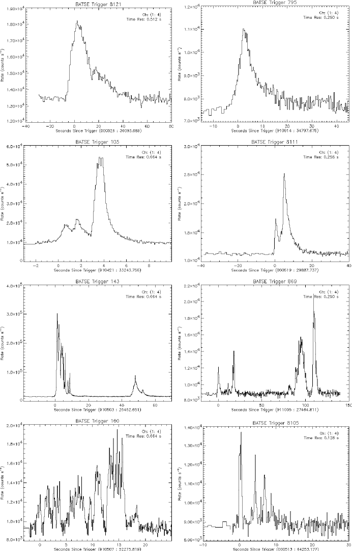
Figure 1: Lightcurve of a few GRBs during prompt emission (Compiled from BATSE catalogue: http://www.batse.msfc.nasa.gov/batse/grb/lightcurve/)

C. Controversial Cases: A New Classification Scheme

The classification scheme as described above got serious challenges from a few observations.

(i) The observation of extended emission in nearly 1/3 rd of the SGRB sample (Lazzati et al. 2001, Connaughton 2002, Norris & Bonnell 2006) renders the definition of $T_{90}$ uncertain. The general feature of extended emission is an initial hard spike, followed by softer emission. The extended emission can last for tens of sec, and thus blurring the demarcation of $T_{90}$ between the LGRB and SGRB class.

(ii) Discovery of two nearby LGRBs (060505, 060614) and one XRF (040701; Soderberg et al. 2005) with no SN association made the matter even more complicated. GRB 060505 (Fynbo et al. 2006) was classified as a nearby ($z=0.089$) LGRB (duration: $4-5$ s, spectral lag: 0.36 s, host: star forming galaxy), but without an observable SN down to deep limit (similar to SGRBs). GRB 060614 (Gehrels et al. 2006) was also a nearby ($z=0.125$) LGRB (duration $\sim 100$ s), without a SN (Fynbo et al. 2006, Della Valle et al. 2006, Gal-Yam et al. 2006). Hjorth & Bloom (2012) suggests that this GRB may be a “failed SN” (Woosley 1993). Alternatively, this can be a short GRB with extended emission (Zhang et al. 2007a). This GRB, except for a longer duration, showed all the characteristics of a short GRB, e.g., negligible delay (Gehrels et al. 2006), low star forming host (Fynbo et al. 2006, Della Valle et al. 2006, Gal-Yam et al. 2006), offset position (Gal-Yam et al. 2006). In fact, Zhang et al. (2007a) have generated a “pseudo-burst” with 8 times lower energy and showed that the synthetic burst is remarkably similar to a short GRB (050724) with extended emission.

(iii) Observation of very distant LGRBs are also puzzling. For example, the LGRB 090423 (Tanvir et al. 2009, Salvaterra et al. 2009) have a spectroscopic $z=8.2$. At this high redshift the cosmological $T_{90}=T_{90}/(1+z)$ would make this a SGRB. However, one should be careful that the classification is based on the observed $T_{90}$, which is a purely phenomenological scheme.

In view of these issues Zhang et al. (2007a) have suggested a new classification scheme. The classical short-hard GRBs are termed as Type I, while the long-soft GRBs are termed Type II. This classification roughly follows the standard SN classification scheme. However, one cannot rule out the possibility of a third category of objects. Incidentally, based on the properties like non-repetition and harder spectrum, GRBs are possibly a different class from SGRs. However, some of the SGRBs may be giant SGR flares from relatively nearby galaxies (Palmer et al. 2005, Tanvir et al. 2005, Abbott et al. 2008, Ofek et al. 2008).

4 Observables

Though there are two classes of GRBs, the radiation properties of them are remarkably similar. Of course, the SGRBs are shorter, harder, and they show dimmer afterglow emission than the LGRBs, which are in fact the distinguishing feature of SGRBs. But, the emission mechanisms are probably similar, and the differences in the observed emission arise due to different environments. Both of them have an initial prompt emission (keV-MeV) phase, followed by softer afterglow in x-rays to optical and radio wavelengths. The prompt and afterglow data of LGRBs have certain advantages over SGRBs: (i) the LGRB sample is much larger than SGRB sample (about 3:1), (ii) LGRBs are brighter and provides better statistics for data analysis, and (iii) due to the longer duration and higher flux, LGRBs are better suited for time-resolved spectroscopy, which is more important than a time-integrated study. Moreover, the analysis done on LGRBs are also applicable for SGRBs, because the emergent spectral and timing properties are likely to be similar. Hence, we shall discuss about LGRBs when analyzing the data. It is worth mentioning that some of the prompt emission properties of these two classes differ, e.g., the spectral lag of SGRBs are much smaller compared to LGRBs (Yi et al. 2006, Norris & Bonnell 2006, Gehrels et al. 2006). Also, SGRBs do not follow the “lag-luminosity” correlation of LGRBs (Norris et al. 2000). These differences may provide useful insight, and can be used for the classification scheme (Gehrels et al. 2006).

1 Prompt Emission Characteristics

A. Lightcurve

During the prompt emission a GRB has a variable lightcurve (LC). Figure 1 shows some LCs compiled from the BATSE website (full BATSE band). Each burst is different from the other. This is in direct contrast with SNe, which have broad similarity of LCs in a class. Close inspection of the LCs in Figure 1 shows multiple pulses in each of them. Following Fishman & Meegan (1995), we can broadly classify the bursts based on their underlying pulse structure as follows.

1. single pulse (or sometimes a spike) events (see the upper most panels)

2. bursts with smoothly overlapping pulses (second panels from the top)

3. bursts with widely separated episodic emission (third panels)

4. bursts with very rapid variability (bottom panels)

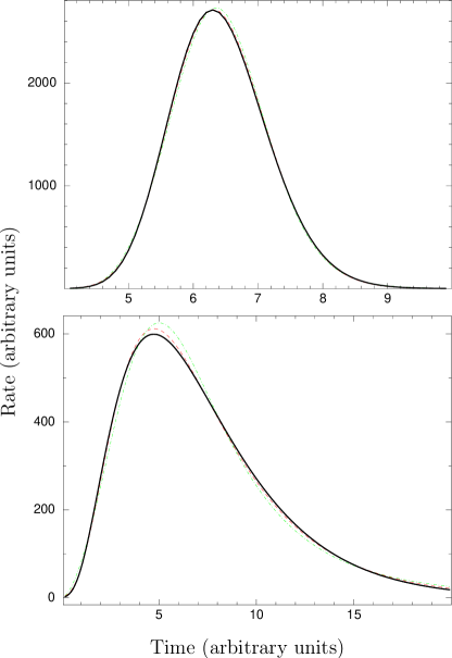
Figure 2: Comparison of FRED (green dot-dashed line), Exponential (black solid line) and lognormal (red dashed line) functions. Upper Panel: Pulse with higher symmetry, Lower Panel: Pulse with higher asymmetry.

It is clear from the LCs that there are broadly two variability scales: slowly varying component, and fast varying component on top of the individual broad variability. Except for the single pulse GRBs, the broad variability time scale is smaller than the total duration of a burst ($T_{\rm GRB}$). The definitions of the variability timescales are rather empirical. A rough estimate of the fast variability can be found by dividing $T_{\rm GRB}$ by the number of peaks in a burst (Piran 1999, cf. Li & Fenimore 1996). This variability timescale has important implication for the working model of a GRB (Kobayashi et al. 1997). In our description of GRBs, we generally assume the rapid variability as “weather” on top of the broad pulse. In a recent study, Xu & Li (2014) have simulated LC for both single variability of Lorentz factor ($\Gamma$) and two-component variability (see Chapter 3 for detail). They have concluded that the latter is preferred to explain the observation of GRB 080319B in both $\gamma$-ray and optical band. The LC in both these bands can be consider as a superposition of a slow varying and a fast varying component. These components are possibly related to the refreshed activity, and the dynamical time scale of the central engine, respectively.

The LC of GRBs are so diverse that no general description is possible. This situation can be simplified by considering the broad constituent pulses. It is suggested that pulses are the basic building blocks of a GRB (Norris et al. 2005, Hakkila et al. 2008). These pulses are (possibly) independently generated in a broad energy band (Norris et al. 2005), and have self-similar shape (Nemiroff 2000). More importantly, GRB pulses have some universal features (Golenetskii et al. 1983, Norris et al. 1986, 1996, Pendleton et al. 1994, Ramirez-Ruiz & Fenimore 2000, Norris 2002, Kocevski & Liang 2003, Norris et al. 2005, Ryde 2005, Hakkila et al. 2008) e.g., the pulses are generally asymmetric, with a sharp rise and slow decay (Kocevski & Liang 2003). Spectrum in a pulse generally exhibit a “hard-to-soft” evolution (e.g., Pendleton et al. 1994). An alternative description of the same behaviour is a negative spectral lag of the hard band with respect to the soft band (i.e., a soft delay). GRB pulses also follow “lag-luminosity” correlation (Norris et al. 2000; see below). In view of these properties, the description of a GRB is equivalent to the description of the constituent pulses. A few empirical functions are available to describe the individual pulses. These are:

• (i) Fast Rise Exponential Decay model (FRED; Kocevski et al. 2003): This pulse shape signifies the phenomenological pulse asymmetry.

  $$F(t)=F_{m}\left(\frac{t}{t_{m}}\right)^{r}\left[\frac{d}{d+r}+\frac{r}{d+r}\left(\frac{t}{t_{m}}\right)^{r+1}\right]^{-\frac{(r+d)}{(r+1)}}$$ (1)

  Here $F_{m}$ is the maximum flux at time, $t_{m}$; $r$ and $d$ are the characteristic indices of the rising and decaying phase, respectively .

• (ii) Exponential model (Norris et al. 2005):

  $$F(t)=A_{n}\lambda{\rm exp}\{-\tau_{1}/(t-t_{s})-(t-t_{s})/\tau_{2}\}$$ (2)

  for $t>t_{s}$. Here $\mu=\left(\tau_{1}/\tau_{2}\right)^{\frac{1}{2}}$ and $\lambda=exp\left(2\mu\right)$. $A_{n}$ is defined as the pulse amplitude, $t_{s}$ is the start time, while $\tau_{1}$, $\tau_{2}$ characteristic times or the rising and falling part of a pulse. One can derive various parameters from these model parameters, e.g., the peak position ($\tau_{\rm peak}$), pulse width ($w$), which is measured as the interval between the two times where the intensity falls to e^-1, and asymmetry of the pulse ($\kappa$).

• (iii) Lognormal distribution (Bhat et al. 2012):

  $$F(t)=\frac{A_{\rm L}}{\sqrt{2\pi}(t-t_{\rm L})\sigma}{\rm exp}\left[-\frac{({\rm log}(t-t_{\rm L})-\mu)^{2}}{2\sigma^{2}}\right]$$ (3)

  for $t>t_{\rm L}$, where $t_{\rm L}$ is the threshold of the lognormal function. Here, $A_{\rm L}$ is the pulse amplitude, $\mu$ and $\sigma$ are respectively the sample mean and standard deviation of log$(t-t_{\rm L})$. The pulse rise time and decay time can be derived from these quantities. The lognormal distribution is motivated by the fact that a parameter, in general, tend to follow a lognormal function if it can be written as a product of $\geq 3$ random variables. It is shown that various GRB parameters follow a lognormal distribution e.g., successive pulse separation (McBreen et al. 1994, Li & Fenimore 1996), break energies of spectra (Preece et al. 2000), and duration of pulses (Nakar & Piran 2002).

In Figure 2, the functions are plotted with arbitrary time axis for a roughly symmetric (upper panel) and an asymmetric pulse (lower panel). Note that though for asymmetric pulse, the FRED profile (green dot-dashed line) tends to have lower width than the other functions, the three models are generally very similar both for a symmetric and asymmetric pulse profile. For asymmetric pulse, the FRED pulse is deliberately drawn with a slightly higher normalization to show its marginal deviation at different parts. However, the deviation is much lower compared to rapid variability of a GRB pulse. Hence, any model can be used as an empirical pulse description. We have chosen Norris model (shown by solid black line) for our later analysis. This function is very similar to the lognormal function.

B. Spectrum

A GRB produces high energy $\gamma$-ray photons in a broad band ($\approx$ 10 keV-10 MeV, with a $\nu F_{\nu}$ peak $\sim 250$ keV). The prompt emission spectrum has a non-thermal shape, or more precisely, the spectrum is not a blackbody (BB). This is generally described by a decaying power-law with photon index $\sim-1$ ($N(\nu)\sim\nu^{\alpha}$, with $\alpha\sim-1$). The spectrum at higher energy can be modelled either as an exponential break or a steeper photon index ($\beta\sim-2.5$) than at the lower energies. Though a GRB has a universal spectral shape, the spectral parameters have a wide range of values.

• The simplest function to describe a GRB spectrum is a power-law (PL; e.g., Fishman & Meegan 1995). Though this can fit a data with a low value of flux, it is generally inapplicable for a spectrum with a high flux. A first order correction to this model is a cut-off power-law (CPL) which has an exponential cut-off at $E_{0}$.

  $$N(E)={\rm cons}\times E^{\alpha}{\rm exp}(-E/E_{0})$$ (4)

• Band function (Band et al. 1993): It is shown that a large number of BATSE GRBs (with high flux) generally require another power-law at higher energy. Band et al. (1993) provides a universal empirical function as:

  $$N(E)=\left\{\begin{array}[]{ll}A_{b}\left[\frac{E}{100}\right]^{\alpha}exp\left[\frac{-(2+\alpha)E}{E_{peak}}\right]\\ $\rm if$~{}~{}E\leq[(\alpha-\beta)/(2+\alpha)]E_{peak}\\ \\ A_{b}\left[\frac{E}{100}\right]^{\beta}exp\left[\beta-\alpha\right]\left[\frac{\left(\alpha-\beta\right)E_{peak}}{100\left(2+\alpha\right)}\right]^{(\alpha-\beta)}\\ {\rm otherwise\par}\end{array}\right.$$ (5)

  This function has two PL indices $\alpha$ and $\beta$ for the lower and higher energies, respectively. The two PL join smoothly (with an exponential roll-over) at a spectral break energy, $E_{\rm break}=[(\alpha-\beta)/(2+\alpha)]E_{peak}$. Apart from the normalization $A_{b}$ and the two photon indices, the break energy or equivalently, the peak energy of $\nu F_{\nu}$ representation is the fourth parameter of the model. Band function is the most discussed spectral function, and it is extensively used to fit GRB spectrum, whether it is time-integrated or time-resolved (e.g., Kaneko et al. 2006, Nava et al. 2011). In Figure 3, we have shown a typical time-resolved (20-23 s bin) spectrum of a GRB (081221), fitted with the Band function (blue line). The $\nu F_{\nu}$ representation (black line) shows the peak of the spectrum ($E_{\rm peak}$). The Band function has some interesting properties: (i) in the limit $\beta\rightarrow-\infty$, the spectrum approaches a CPL function, (ii) as $\alpha\rightarrow\beta$, the spectrum approaches a PL, and (iii) the value of $\alpha$ can be directly used to interpret the possible radiation mechanism.

• Other than these functions, a few more functions are discussed in the literature. For example, a broken PL (Schaefer et al. 1992), lognormal (Pendleton et al. 1994), optically thin bremsstrahlung spectrum with a PL, and smoothly broken PL (SBPL; Preece et al. 1996). However, the Band function is regarded as the most appropriate standard function of GRBs.

In recent years, a few new functions are suggested for the spectral description, e.g., a BB with a PL (BBPL; Ryde 2004), multicolour BB with a PL (mBBPL; Pe’er 2008), BB+Band (Guiriec et al. 2011), two BB with a PL (2BBPL; Basak & Rao 2013b). The general feature of these models is that the spectrum is decomposed into a thermal (either one BB, or mBB, or two BBs) and a non-thermal (PL, Band etc.) component. The aim of these models is obtaining a physical insight of the spectrum, which is not provided by an empirical Band function. We shall discuss more about the alternative models in chapter 4.

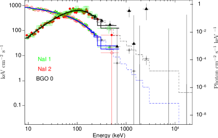
Figure 3: Time-resolved spectrum (20-23 s post trigger) of GRB 081221. Both the photon spectrum (shown by blue histogram fitting) and the corresponding $\nu F_{\nu}$ representation (shown by black histogram fitting) are shown. This spectrum is extracted from Fermi data. The different detectors are shown by different colours. The data is fitted using Band function (Band et al. 1993) with $\alpha=-0.32^{+0.08}_{-0.08}$, $\beta=-3.65^{+0.40}_{-1.2}$ and $E_{\rm peak}=106^{+4.3}_{-4.0}$ keV. The errors quoted are at nominal 90% confidence.

C. Spectral evolution

It is found that a GRB spectrum rapidly evolves during the prompt emission. Hence, time-resolved spectral study is more important than the time-integrated study. Within the individual pulses of most of the bursts, $E_{\rm peak}$ evolves from high to low values, commonly described as a “hard-to-soft” (HTS) evolution (e.g., Pendleton et al. 1994, Bhat et al. 1994, Ford et al. 1995, Liang & Kargatis 1996, Kocevski & Liang 2003, Hakkila et al. 2008; see Hakkila & Preece 2014 for a recent discussion). It is suggested that the HTS spectral evolution is a pulse property. However, this feature is questioned in a few studies. For example, Lu et al. (2012) have studied $E_{\rm peak}$ evolution in a set of 51 long and 11 short GRBs. Though they have found HTS pulses, a substantial number of GRBs also show a “intensity tracking” (IT) behaviour. They have found that the first pulses are generally HTS, but later pulses tend to follow an IT behaviour rather than a HTS evolution. They have suggested that some of these IT pulses might have contamination effect from an earlier HTS pulse. However, the fact that some of the single pulse GRBs also show IT behaviour cannot be explained by an overlapping effect. Note that IT evolution can be considered as a “soft-to-hard-to-soft” evolution. These issues will be discussed in Chapter 4, when we will deal with alternative spectral models and their evolution.

2 Generic Features Of Afterglows

The prompt emission is followed by an afterglow phase, which progressively becomes visible in x-ray, optical and some times in radio wavelengths. These emissions last on time scales of days to months, with longer duration in the longer wavelengths. Unlike the prompt emission, which has rapid variability in the LC, the afterglow is a smooth function of time, decreasing as a PL ($F_{\nu}(t)=t^{\alpha_{A}}\nu^{\beta_{A}}$, with $\alpha_{A}=-1.1$ to $-1.5$ and $\beta_{A}=-0.7$ to $-1.0$; Mészáros 2006). A wealth of x-ray afterglow data is provided by the Swift/XRT (Burrows et al. 2005b; also see Evans et al. 2007, 2009). One of the most important discoveries of the XRT is finding a canonical behaviour for all bursts, from as early as 100 s till a few days (Chincarini et al. 2005, Nousek et al. 2006, Zhang et al. 2006, O’Brien et al. 2006), which consists of three phases (see Zhang 2007a, b for detail): a steep decay ($10^{2}-10^{3}$ s with an index $\gtrsim-3;~{}F_{X}(t)\sim t^{\alpha_{XA}}$), followed by shallow decay ($10^{3}-10^{4}$, with an index -0.5), and then a normal decay phase ($\alpha_{XA}\sim-1.2$). Other than these phases, an occasional “post jet break phase”, and in nearly 50% cases, one or more x-ray flares are seen (Burrows et al. 2005a). Kann et al. (2010) have compiled a list of optical afterglow data and have shown that the data is consistent with the standard model. Chandra & Frail (2012) have reported a total of 304 bursts which were observed with very large array (VLA). They found $\sim$ 31% having radio, $\sim$ 65% having optical and $\sim$ 73% having detected x-ray afterglow. The reason that many GRBs do not show radio afterglow is attributed to synchrotron self absorption in the initial phase of the radio afterglow.

An important feature of the afterglow lightcurve is an achromatic break (Fruchter et al. 1999, Kulkarni et al. 1999, Stanek et al. 1999, Harrison et al. 1999, Frail et al. 2001). This break is claimed as the smoking gun signature of a jet. In other words, a GRB is probably a collimated event rather than a fully isotropic emission, and they are detected only when the jet points towards the observer. Note that, this assumption reduces the energy requirement, and increases the population of GRBs, both by a factor of $\approx 100$.

3 GeV Emission

Apart from the keV-MeV emission and later x-ray, optical and radio emission, GRBs are also accompanied by very high energy (GeV) emission (Hurley et al. 1994). GeV emission appears during the prompt phase, generally starting with a delay with respect to the keV-MeV emission, and lasts longer than the prompt emission phase. The later evolution of GeV flux resembles an afterglow behaviour. In fact, Kumar & Barniol Duran (2010) have shown that the evolution of GeV flux can correctly predict the later x-ray and optical afterglow flux. However, the origin of this emission is debatable (Meszaros & Rees 1994, Waxman 1997, Fan & Piran 2008, Panaitescu 2008, Zhang & Pe’er 2009, Mészáros & Rees 2011), and remains unknown during the prompt emission phase.

The spectrum containing the full MeV-GeV band has either an overall Band functional shape (Dingus et al. 1998), or sometimes an additional PL is required to fit the spectrum (e.g., González et al. 2003) For the last 5 years, a great amount of GeV data is being provided by Fermi/LAT (Atwood et al. 2009). The LAT detects high energy (GeV) emission in a wide band of 30 MeV to 300 GeV (see Chapter 2 for details). More than 35 GRBs with GeV photons have been detected by the LAT so far (Abdo et al. 2009d, Ackermann et al. 2013). The broadband data of the Fermi/GBM and the Fermi/LAT has provided various clues both in the GRB science and in basic physics, e.g., (i) detection of distinct spectral components and their evolution (Abdo et al. 2009c, b), (ii) detection of $\gamma$-ray photons of energy of up to 30 GeV constraining the bulk Lorentz factor ($\Gamma$) to be greater than $\sim 1000$ (Abdo et al. 2009c, Ghirlanda et al. 2010a), and (iii) discovery of GeV photons in the SGRB 090510 which helps to put a stringent limit on the possible violation of Lorentz invariance (Abdo et al. 2009a).

4 GRB Correlations

One of the most important, and promising ingredients in understanding the physics of a GRB is empirical correlations during the prompt emission. Though the underlying physical reason of the correlations are not always clear, any prompt emission model should successfully reproduce the data driven empirical correlations. Hence, correlation study can put some constraint on the possible models. Another more ambitious goal of the correlation study is using GRBs as cosmological luminosity indicators. One of the greatest discovery in modern cosmology is the finding of the accelerated expansion of the universe, using high-$z$ type Ia SN (SN Ia) as standard candle (Schmidt et al. 1998, Riess et al. 1998, Perlmutter et al. 1999; 2011 Nobel Prize in Physics). From the theoretical absolute luminosity and the observed luminosity the luminosity distance is derived to measure the acceleration, the amount of dark and baryonic matter ($\Omega_{m}$), and dark energy ($\Omega_{\Lambda}$) in $\Lambda$ cold dark matter cosmology model ($\Lambda$-CDM). However, due to the absorption of optical light, SN cannot be seen at high $z$ (maximum $z\leqslant 1.755$; Riess et al. 2007). On the other hand, GRBs being very luminous in $\gamma$-rays, are visible from very large distances. Hence, they are considered as potential luminosity indicators beyond this redshift limit. However, unlike SN Ia, the GRB energetics is not standardized. Though Frail et al. (2001) and Bloom et al. (2003), using the pre-Swift data have shown that GRBs are standard energy reservoir, this is discarded with systematic observations by Swift (Willingale et al. 2006, Zhang et al. 2007b). In addition, the radiation mechanism of a GRB is also uncertain. Hence, with no other options in hand, the empirical correlations are the only way to study GRBs as a cosmic ruler.

GRB correlations are studied either in time or in energy domain. For example, the $\nu F_{\nu}$ peak energy ($E_{\rm peak}$) correlates with the $\gamma$-ray isotropic energy ($E_{\gamma,\rm iso}$), known as Amati correlation (Amati et al. 2002, Amati 2006, Amati et al. 2009). $E_{\rm peak}$ also correlates with isotropic peak luminosity ($L_{\rm iso}$; Schaefer 2003, Yonetoku et al. 2004), and collimation-corrected energy ($E_{\gamma}$; Ghirlanda et al. 2004b). In the time domain, the correlations are e.g., spectral lag ($\tau_{\rm lag}$) - $L_{\rm iso}$ (Norris et al. 2000), variability (V) - $L_{\rm iso}$ (Fenimore & Ramirez-Ruiz 2000, Reichart et al. 2001), and rise time ($\tau_{\rm rise}$) - $L_{\rm iso}$ (Schaefer 2007). It is worthwhile to mention that several apparent correlations can arise due to the instrumental selection effect (e.g., Nakar & Piran 2005, Band & Preece 2005). One argument against the selection bias is to show that the correlation exists within the time-resolved data of a given burst (e.g., Ghirlanda et al. 2010b). In chapter 3, based on a new pulse model, we shall introduce a new GRB correlation (Basak & Rao 2012a). We shall primarily discuss the correlations studied in the energy domain. We shall also discuss about how the new correlation exists against the selection bias. In Table 2, we have summarized the correlations. Here, N is the number of bursts, $\rho$, $r$ are Spearman rank, Pearson linear correlation, respectively. P is the chance probability. The corresponding relations are shown in the last column.

The quantities are defined as follows.

Table 2: Correlations in GRBs

Correlation	N	$\rho$/$r$	P	Relation
${}^{(a)}E_{\rm peak}$-$E_{\gamma,\rm iso}$	9	$\rho=0.92$	$5.0\times 10^{-4}$	$\frac{E_{\rm peak}}{1~{}\rm keV}$=$(105\pm 11)\left[\frac{E_{\gamma,\rm iso}}{10^{52}\rm erg}\right]^{0.52\pm 0.06}$
${}^{(b)}E_{\rm peak}$-$E_{\gamma,\rm iso}$	41	$\rho=0.89$	$7.0\times 10^{-15}$	$\frac{E_{\rm peak}}{1~{}\rm keV}$=$(81\pm 2)\left[\frac{E_{\gamma,\rm iso}}{10^{52}\rm erg}\right]^{0.57\pm 0.02}$
${}^{(c)}E_{\rm peak}$-$L_{\rm iso}$	16	$r=0.958$	$5.31\times 10^{-9}$	$\frac{10^{5}L_{\rm iso}}{10^{52}\rm erg~{}s^{-1}}$=$(2.34_{-1.76}^{+2.29})\left[\frac{E_{\rm peak}}{1~{}\rm keV}\right]^{2.0\pm 0.2}$
${}^{(d)}E_{\rm peak}$-$E_{\gamma}$	27	$\rho=0.80$	$7.6\times 10^{-7}$	$\frac{E_{\rm peak}}{1~{}\rm keV}$=$(95\pm 7)\left[\frac{E_{\gamma}}{10^{52}\rm erg}\right]^{0.40\pm 0.05}$

^aThe original Amati correlation (Amati et al. 2002). ^bAmati (2006), ^cYonetoku et al. (2004), ^dGhirlanda et al. (2004b)

Let us assume that the observed fluence (time integrated flux) is $S_{\rm obs}$ and peak flux is $P_{\rm obs}$. The k-corrected bolometric fluence and peak flux are:

$$S_{\rm bolo}=S_{\rm obs}\times\frac{\int_{1/1+z}^{10^{4}/1+z}E\times N(E)dE}{\int_{E_{\rm min}}^{E_{\rm max}}E\times N(E)dE}~{}~{}~{}\rm erg~{}cm^{-2}$$ (6)

and

$$F_{\rm bolo}=P_{\rm obs}\times\frac{\int_{1/1+z}^{10^{4}/1+z}E\times N(E)dE}{\int_{E_{\rm min}}^{E_{\rm max}}E\times N(E)dE}~{}~{}~{}\rm erg~{}cm^{-2}~{}s^{-1}$$ (7)

Here, the integration in the numerator are done in the energy band 1 keV to $10^{4}$ keV in the source frame. The spectral function $N(E)$ is generally taken as the Band function. In the denominator, the integration is done over the instrument band width. The ratio of these fluxes give the bolometric k-correction. The $\gamma$-ray isotropic energy ($E_{\gamma,\rm iso}$) and isotropic peak luminosity ($L_{\rm iso}$) are defined as:

$$E_{\gamma,\rm iso}=4\pi d_{\rm L}^{2}\frac{S_{\rm bolo}}{1+z}~{}~{}~{}\rm erg$$ (8)

and

$$L_{\rm iso}=4\pi d_{\rm L}^{2}F_{\rm bolo}~{}~{}~{}\rm erg~{}s^{-1}$$ (9)

Here $d_{\rm L}$ is the luminosity distance of the source, which is dependent on $z$ and the version of cosmology in use. Generally, a $\Lambda$-CDM cosmology with a zero curvature ($\Omega_{K}=0$), ($\Omega_{m}$, $\Omega_{\Lambda}$)=(0.27, 0.73), and Hubble parameter, $H_{0}=70$ km s^-1 Mpc^-1 is used.

If a GRB is a jetted event, then the energy of the source is corrected for the collimation. If $\theta_{j}$ is the half opening angle, then the collimation corrected energy is

$$E_{\gamma}=(1-{\rm cos}\theta_{j})E_{\gamma,\rm iso}$$ (10)

5 A Working Model for GRBs

In this section, we shall briefly discuss the working model of GRBs. The basic ingredients of this model are known, however, quantitative calculations are still lacking. In addition, several modifications of the radiation process, emission region, and even completely different models are also proposed. For a detailed description of the standard model see reviews by Piran (1999) and Mészáros (2006). For later purpose, we shall use notation $q_{x}$ to denote a quantity $q$ in the cgs units of $10^{x}$. For example, $E_{52}$ is $E$ in the units of $10^{52}$ erg.

1 Compactness And Relativistic Motion

From the discussion of the prompt emission features, we know that a GRB has rapid observed variability ($\delta t_{\rm obs}\approx$ 1 s down to 10 ms), and an enormous observed flux. A cosmological distance translates the observed flux to high luminosity ($L_{\rm iso}\sim 10^{53}~{}\rm ergs^{-1}$). This particular combination has a very important consequence, known as compactness problem. From the variability argument, the emission radius has an upper limit, $R_{\rm s}<c\delta t_{\rm obs}\sim 10^{8}$ cm. Hence, the compactness parameter, $\sigma_{\rm T}L_{\rm iso}/R_{\rm s}m_{\rm e}c^{3}\gg 1$. In other words, a huge number of photons are created in a small volume of space. Hence, the photons will pair produce leading to a spectral cut-off precisely at 512 keV, the rest frame energy of an electron ($m_{e}c^{2}$). This is in direct contradiction with the observed spectrum, which contains many photons in the range 0.5 MeV-10 MeV (sometimes extending to even GeV energies).

The compactness will lead to rapid pair production ($\gamma\gamma\rightarrow e^{-}e^{+}$), and hence a high optical depth is attained. If $f_{\rm p}$ is the fraction of photon pairs which satisfy the pair production criteria, then for a source with an observed flux $F$, distance $d$, and variability $\delta t$ has an average optical depth (Piran 1999),

$$\tau_{\gamma\gamma}=10^{13}f_{\rm p}\left[\frac{F}{10^{-7}~{}{\rm erg~{}cm^{-2}}}\right]\left[\frac{d}{3Gpc}\right]^{2}\left[\frac{\delta t}{10~{}\rm ms}\right]^{-2}$$ (11)

Note that the compactness problem is an unavoidable consequence of the cosmological origin of GRBs — the severity of the situation essentially increases with increasing distance. In fact, this was one of the most important arguments against the cosmological origin (Ruderman 1975, Schmidt 1978, Cavallo & Rees 1978). During late 1950’s to mid-1960’s, astronomers faced a similar inconsistency in quasars. From the observed line ratios in the optical spectrum the distance was found to be cosmological. The variability of a typical quasar is $\sim$ day, which indicates a compact region. With this high compactness the sources should lead to “Compton catastrophe”, and no radiation should be seen. This even led to the proposal of discarding the extra-galactic origin of quasars (Hoyle 1966). The cosmological distance scale of quasars was saved by implementing ultra-relativistic expansion of the sources (Woltjer 1966, Rees 1967). Later observation with Very Large Baseline Array (VLBA) confirmed the apparent superluminal motion of quasar jets with bulk Lorentz factor, $\Gamma\approx 2-20$. Similar situation with even more severity occurred for GRBs. The solution was also similar (see Katz 2002 for detail).

The relativistic motion with a bulk Lorentz factor has three effects which help GRBs bypassing the compactness problem.

• (i) Due to the relativistic effect an observed photon will have a blue shifted observed energy ($h\nu_{\rm obs}$). The energy in the source frame can be obtained as $h\nu_{\rm obs}/\Gamma$. This will enormously reduce the fraction of photons eligible for pair production in the source frame. This factor is $\Gamma^{2\beta}$, where $\beta$ is the high energy spectral index. Note that for simplicity, we have neglected the cosmological redshift correction of the source frame energy, which is much smaller compared to the correction discussed above.

• (ii) For an observer, the arrival time of two successive pulses will be compressed as the source generating the pulses moves with high $\Gamma$. Hence, the emission radius is allowed to be larger than $R_{\rm s}<c\delta t_{\rm obs}$ by a factor $\Gamma^{2}$.

• (iii) The pair production threshold for a head-on interaction for two photons with energy $E_{1}$ and $E_{2}$ is $\sqrt{E_{1}E_{2}}>m_{e}c^{2}$. For a relativistic source, the radiation will be beamed, and the photons will interact only in grazing angles with each other. This increases the pair production threshold to an arbitrary higher value (Katz 2002).

The optical depth using these correction factors is $\tau^{\rm(ac)}\sim\frac{\tau_{\gamma\gamma}}{\Gamma^{4+2\beta}}$. Putting the actual numbers, one gets a lower limit on $\Gamma>100$ (Piran 1999). An alternative approach also gives a similar $\Gamma>100[(E_{1}/10~{}\rm GeV)(E_{2}/\rm MeV)]^{1/2}$, where $E_{1}$ is the energy (in 10 GeV) of a high energy photon that escapes annihilation with a lower energy target photon of energy $E_{2}$ MeV. Following Mészáros (2006), the following notations will be used:

• $K_{*}\rightarrow$ Origin of the explosion (lab frame), $K^{\prime}\rightarrow$ Co-moving frame of the gas (fireball), $K\rightarrow$ Observer frame

• $dr_{*}=dr=\frac{dr^{\prime}}{\Gamma}\rightarrow$ Usual length contraction

  $dt_{*}=dt^{\prime}\Gamma\rightarrow$ Usual time dilation

  $dt_{*}=\frac{dr_{*}}{\beta c}\approx\frac{dr_{*}}{c}\rightarrow$ Time separation between successive events. $\beta=v/c$

  $dt=dt_{*}(1-\beta)\rightarrow$ Time separation between events (in observer frame)

• Transformation from $K^{\prime}$ to $K$ is done by Doppler factor which is defined as $D\equiv\left[\Gamma(1-\beta\mu)\right]^{-1}$. Here, $\mu=\rm cos\theta$, where $\theta$ is the angle between the expansion direction of the ejecta and the line of sight towards the observer. Some examples of transformations are: time transformation: $dt=D^{-1}dt^{\prime}$ (combining second and fourth relations), frequency transformation: $\nu=D\nu^{\prime}$. For $\Gamma\gg 1$, and $\mu\rightarrow 1$ (approaching), $D\approx 2\Gamma$, and $\mu\rightarrow-1$ (receding), $D\approx 1/2\Gamma$

2 “Fireball Model” And Radiation Mechanism

A. Photon-Lepton Fireball

The first major attempt to explain the consequences of a cosmological distance on the dynamics and spectral features during the prompt emission of a GRB was proposed in two independent papers by Goodman (1986) and Paczynski (1986). Note that these papers were published even before the BATSE was launched. Both the authors start with the assumption that GRBs have cosmological origin, and hence from the observed flux their luminosity must be high, in fact much higher than the Eddington luminosity ($L_{\rm E}=1.25\times 10^{38}(M/M_{\odot})~{}{\rm erg~{}s^{-1}}$). Hence, the radiation pressure largely exceeds the self-gravity, leading to an expansion of the source. In this model, the ejecta is considered to be a purely photon-lepton ($\gamma-e^{-}/e^{+}$) opaque plasma, referred to as a “fireball”.

Let us assume that in a region of size $r_{\rm i}$, a huge energy $E_{\rm i}$ is created, and the mass of the system, $M_{\rm i}\ll E_{\rm i}/c^{2}$. As the fireball expands, the co-moving temperature ($T^{\prime}$) decreases due to an adiabatic cooling. As the fireball is radiation dominated, the adiabatic index, $\gamma_{a}=4/3$. Hence, the cooling law is, $T^{\prime}\propto r^{-1}$, where $r$ is the radius of the fireball measured from observer frame. Note that $r$ is the same as measured from the stationary lab frame, $K_{*}$. As temperature decreases, the random Lorentz factor ($\gamma_{\rm r}$) also drops ($\gamma_{\rm r}\propto r^{-1}$). Hence, from energy conservation, the internal energy per particle is continuously supplied for expansion energy, i.e., $\gamma_{r}\Gamma=\rm constant$. Hence, $\Gamma$ increases linearly with $r$. However, the acceleration cannot go on for ever. When the bulk kinetic energy ($\Gamma M_{\rm i}c^{2}$) becomes equal to $E_{\rm i}$, the value of $\Gamma$ ceases to increase. From the relation, $\Gamma_{\rm max}M_{\rm i}c^{2}=E_{\rm i}$ one can obtain this coasting value as $\Gamma_{\rm max}\sim\eta\equiv E_{\rm i}/M_{\rm i}c^{2}$. Here, $\eta$ is called the dimensionless entropy of the fireball. The value of $\eta$ determines the coasting value of $\Gamma$. The time evolution of $\Gamma$ can be written as follows (see Mészáros 2006):

$$\Gamma(r)\sim\left\{\begin{array}[]{ll}(r/r_{\rm i})&\mbox{ for $r<r_{\rm s}=\eta r_{\rm i}$}\\ \eta&\mbox{ otherwise}\end{array}\right.$$ (14)

The comoving temperature can be shown to vary as follows:

$$kT^{\prime}(r)\sim\left\{\begin{array}[]{ll}(r/r_{\rm i})^{-1}&\mbox{ for $r<r_{\rm s}$}\\ (r/r_{\rm i})^{-2/3}&\mbox{ otherwise}\end{array}\right.$$ (17)

Here $r_{\rm s}$ is called the saturation radius (where $\Gamma$ attains the maximum value and the acceleration stops). Another important parameter is the photospheric radius ($r_{\rm ph}$), which is defined as the radius where the photons decouple from the matter. Within $r_{\rm ph}$, the energy of the photons is continuously converted into the kinetic energy of the fireball. The fireball remains optically thick (optical depth, $\tau>1$) below this radius. The optical depth to Thomson scattering in the radial direction from a radius ($r$) to infinity is

$$\tau=\int_{r}^{\infty}{\rho^{\prime}(r^{\prime})\kappa D^{-1}dr^{\prime}}$$ (18)

Here, $\kappa=\sigma_{\rm T}/m_{p}$ ($\sigma_{\rm T}$ is Thomson scattering cross section, $m_{p}$ is proton mass) is the total mass opacity, and $\rho^{\prime}$ is the co-moving density. The value of $r_{\rm ph}$ can be found by putting $\tau=1$ in equation 18. If $\dot{M}$ is the mass injection rate, then $\rho^{\prime}=\frac{1}{\Gamma}\frac{\dot{M}}{4\pi r^{2}\beta c}=\frac{L}{\Gamma 4\pi r^{2}\beta\eta c^{3}}$ (as $\eta=E_{\rm i}/M_{\rm i}c^{2}=L/\dot{M}c^{2}$). Using these values in equation 18, and putting $\tau=1$ for $r=r_{\rm ph}$, we get

$$r_{\rm ph}=\frac{\sigma_{\rm T}L}{8\pi\eta^{3}m_{p}c^{3}}$$ (19)

The observer frame temperature ($kT$) can be found by $kT\sim\Gamma kT^{\prime}$. Using equation 14 and 17, we obtain,

$$kT(r)\sim\left\{\begin{array}[]{ll}{\rm constant}&\mbox{ for $r<r_{\rm s}$}\\ (r/r_{\rm i})^{-2/3}&\mbox{ otherwise}\end{array}\right.$$ (22)

If the photosphere occurs higher than the saturation radius ($r_{\rm ph}>r_{\rm s}$), an observer will see a hard-to-soft (or rather a hot-to-cold) evolution. However, the spectral peak and luminosity will be degraded. On the other hand, for $r_{\rm ph}>r_{\rm s}$, a break is expected in the $E_{\rm peak}$ (or rather kT) evolution. However, note that the spectrum predicted by the model is a blackbody (BB — Planckian spectrum), rather than a Band function. A BB has a photon index $+1$, in the lower energy, while a typical GRB has a $-1$ photon index. In other words, a BB spectrum is too hard for GRBs. Also, in the high energy part of the spectrum, while a BB has an exponential fall off, the Band function falls only as a PL with an index $\sim-2.5$. A typical GRB has a wider peak than a BB. Goodman (1986) proposed a geometric broadening of the BB spectrum due to the finite size of the photosphere. However, the proposed modified BB cannot account for the very different shape of a GRB spectrum. Though this model cannot explain the spectral features, it gives the essential ingredient to achieve relativistic motion in a GRB. In recent years, modified forms of photospheric emission has received considerable attention (e.g., Ryde 2004, 2005, Pe’er et al. 2005, 2006; see also Mizuta et al. 2011, Lazzati et al. 2013). We shall discuss more about these models in chapter 4.

B. Baryon Loading And Internal-External Shock Paradigm

The failure of the photon-lepton fireball led researchers to try some modifications of the basic assumptions. The first logical step was to introduce baryons in the otherwise pure photon-lepton plasma (Shemi & Piran 1990). A baryon loaded fireball has two major modifications on the original fireball: (i) As the $M_{\rm i}$ is larger, the coasting Lorentz factor, $\eta=E_{\rm i}/M_{\rm i}c^{2}$ is lower. Of corse, the baryon load should not be so high that the ultra-relativistic motion (which is required by observation) is killed. Such a situation occurs in supernova explosion, where the baryon load leads to a non-relativistic motion of the ejecta ($<0.1c$). (ii) If the baryon load $M_{\rm b}$ exceeds the value $M_{\rm critical}=2\times 10^{-7}M_{\odot}E_{52}^{2/3}r_{\rm i7}^{2/3}$ (where $E_{52}$ is $E$ in units of $10^{52}$ erg, $r_{\rm i7}$ is $r_{\rm i}$ in units of $10^{7}$ cm), then the fireball becomes matter dominated before it reaches the photosphere (in this case, a baryonic photosphere rather than a pair photosphere is formed). The internal energy will be mostly converted into kinetic energy of the baryons, and no radiation will be seen at the photosphere. Hence, the outcome of a baryon loaded fireball is a “clothed fireball”.

It is worthwhile to mention that if the baryon load is less than $\sim 10^{-12}M_{\odot}E_{52}^{1/2}r_{\rm i7}^{1/2}$, the baryon will have negligible effect. With $M_{\rm b}<M_{\rm critical}$, still the fireball will be radiation dominated, with a degraded temperature. Certainly, in order to avoid producing a thermal spectrum the feasible choice is $M_{\rm b}>M_{\rm critical}$. But, the energy is then drained by the baryons leading to no radiation. However, this energy is available in the form of kinetic energy of the baryons. Hence, in order to produce a GRB, the kinetic energy must be made available in the form of radiation. Rees & Meszaros (1992) and Meszaros & Rees (1993) proposed a mechanism to reconvert the kinetic energy into radiation. This model involves shock generation in the external circumburst medium, and it is known as the “External shock” (ES) model. The essential idea is that the fireball plasma cannot move with constant velocity for ever, and when it eventually plunges into the external medium, it heats up the gas, “sweeps up” mass and decelerates. The external medium can be either a pre-ejected wind of the progenitor, or the interstellar medium (ISM). The interaction process is mediated via “collisionless” turbulent plasma shock wave rather than direct particle collision. This shock is commonly referred to as the “External shock”. This shock is expected because of the discontinuity of density, temperature and pressure between the fireball plasma and the ISM plasma. The detailed mechanism of a turbulent plasma shock is incalculable, but it is believed that a part of the energy is used to accelerate electrons to very high $\gamma_{e}$, and another part is converted to magnetic field. The electrons can gyrate in the magnetic field producing synchrotron radiation. As a synchrotron spectrum is non-Planckian with a wider peak in the $\nu F_{\nu}$ representation, it naturally explains the observed spectrum of a GRB. This process will produce a single pulse with a fast rise and a slow decay. The complex LC of a GRB can be produced by assuming density fluctuations (clumps) in the ISM. The requirement of this hypothesis is that the clumps should be small and sparsed, otherwise the temporal fluctuation will not be observed (Piran 1999). However, the clumps are required to be so small and sparsed that it will be very unlikely to have multiple collisions in the line of sight. Hence, ES can make only a faint burst with a single pulse by interacting with a clumpy ISM. Even if continuous collisions happen (e.g., in a relatively uniform density ISM), due to the deceleration of the fireball (decreasing $\Gamma$): (i) the spectrum should have a hard-to-soft evolution, and (ii) the later sub-pulses should be more stretched out in the observer frame. Though a hard-to-soft evolution is common in a GRB, the sharpness of the individual sub-pulses is independent of their time sequence. Note that this model was proposed before the afterglow era. Following the detections of afterglows (from 1997 onwards), it became apparent that the predictions of ES model are compatible with afterglow features. Hence, it was suggested that the ES can give rise to the afterglow rather than the prompt emission phase. In fact, the features of the afterglow data matches quite well with the ES predictions — hard-to-soft evolution, and longer duration in lower energies (e.g., Mészáros & Rees 1997, Reichart 1997, Waxman 1997, Vietri 1997, Tavani 1997, Wijers et al. 1997). In addition to the forward external shock as described above, a “reverse shock” may generate which propagates back into the material behind the shock front (Sari & Piran 1999a). The signature of such a shock is found as an optical/UV flash during the afterglow for a handful of GRBs (e.g., Sari & Piran 1999b).

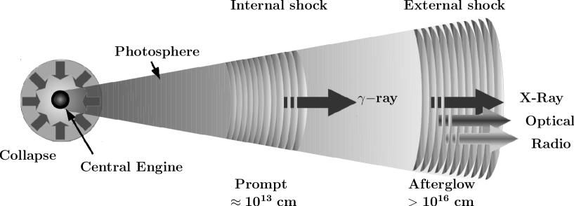
Figure 4: Model of Gamma-Ray Bursts, re-drawn following Mészáros (2001)

Rees & Meszaros (1994) proposed another possible site for energy dissipation. They pointed out that the central compact object, which has a dynamical time scale $\sim$ milliseconds, releases fireshells with varying Lorentz factors ($\Gamma$), instead of a steady ejecta. If a fast moving shell catches up with a slower one, it generates “internal shock” (IS). If two successive shells of same mass but different Lorentz factors ($\Gamma_{1}$ and $\Gamma_{2}$) are ejected on a timescale $\delta t_{\rm var}$ (in the lab frame), then the radius where ISs build up is $\sim c\delta t_{\rm var}\Gamma_{1}\Gamma_{2}$. The ISs accelerate electrons which will generate synchrotron spectrum. The IS model can explain the complex LC, and the non-thermal spectrum of a GRB. However, it does not predict anything about the spectral evolution. Also, due to the fact that both the shells are moving out in the same direction, their relative velocity is small, and consequently, the efficiency of energy conversion is low compared to the ES case. If $\Gamma_{\rm f}$ and $\Gamma_{\rm s}$ are a pair of fast moving and slow moving shells which collide to form a final shell with $\Gamma_{\rm t}=\sqrt{\left(\Gamma_{\rm f}\Gamma_{\rm s}\right)}$, then the efficiency is $\epsilon=\left(\Gamma_{\rm f}+\Gamma_{\rm s}-2\sqrt{\Gamma_{\rm f}\Gamma_{\rm s}}\right)/(\Gamma_{\rm f}+\Gamma_{\rm s})\sim 20\%$.

In Figure 4, we have shown the schematic view of the IS-ES model (Mészáros 2001). This is the most widely discussed model of GRB radiation (e.g., Rees & Meszaros 1992, 1994, Katz 1994b, Sari & Piran 1997).

Some modifications of the ingredients of the prompt emission mechanism do exist. For example, a magnetically dominated ejecta is expected to produce prompt emission via magnetic reconnection (Usov 1992, 1994, Metzger et al. 2007, Metzger 2010; see also Zhang & Yan 2011: Internal-Collision-induced MAgnetic Reconnection and Turbulence, ICMART). Such a mechanism will have different emission radius and spectral evolution. The prompt emission is likely to be followed by a similar afterglow due to ES of the standard model. The only difference would be that due to a very high Alfvén speed of the ejecta, the reverse shock will be absent (or weak). The prompt emission is expected to be highly polarized. A completely different model, called “cannon-ball model” (CB), is proposed by Dado et al. (2002, 2007), Dar & de Rújula (2004), Dar (2006). This model advocates particle interaction, rather than shock wave generation. The central engine shoots out CBs of ordinary matter which produce prompt emission via bremsstrahlung, and afterglow via inverse Compton (IC) of the ambient photon field.

C. Locations

In the standard fireball model the radiation can arise from several regions. In addition to the standard IS and ES regions the photosphere can also contribute to the radiation (see chapter 4). By putting the actual numbers, the locations of these emissions can be estimated (Mészáros 2006) as follows.

• The photospheric radius,

  $$r_{\rm ph}\sim 6\times 10^{11}L_{51}\eta_{2}^{-3}~{}\rm cm$$ (23)

  The baryonic photosphere can occur below or above this radius depending on the baryon load.

• The radius where ISs develop is,

  $$r_{\rm IS}\sim c\delta t_{\rm var}\eta^{2}\sim 3\times 10^{13}\delta t_{\rm var,-1}\eta_{2}^{2}~{}\rm cm$$ (24)

  Here $\delta t_{\rm var,-1}$ is $\delta t_{\rm var}$ in units of 0.1 s.

• The radius where ESs develop is,

  $$\begin{split}r_{\rm ES}&\sim(3E_{i}/4\pi n_{ext}m_{p}c^{2}\eta^{2})^{1/3}\\ &\sim 5.5\times 10^{16}E_{53}^{1}/3n_{ext}\eta_{2.5}^{-2/3}~{}\rm cm\end{split}$$ (25)

D. Achromatic Breaks And Evidence Of Jet

One of the most important observations of GRB afterglow is the achromatic break in the LC. This is claimed as the evidence of GRB jets (Fruchter et al. 1999, Kulkarni et al. 1999, Stanek et al. 1999, Harrison et al. 1999, Frail et al. 2001; cf. Sari et al. 1999). In fact, a LC break is predicted for a jet due to the following relativistic effect (Rhoads 1997, 1999). If $\Gamma$ is the bulk Lorentz factor of the source, then an observer can see only $1/\Gamma$ portion of the ejecta. As the ejecta decelerates in the external medium, $\Gamma$ decreases. Thus an observer tends to see more an more portion of the ejecta i.e., the light-cone becomes wider. If the ejecta is totally isotropic, then the observed flux decreases steadily as a combination of decreasing flux and increasing accessible area that an observer sees. However, for a physical jet with an opening angle $\theta_{j}$ (or a solid angle $\Omega_{j}$), this situation will be different. If an observer is within $\Omega_{j}$ and as long as $\Gamma\gtrsim\Omega_{j}^{-1/2}$, the observer is unaware of the physical structure. But, as soon as $1/\Gamma$ becomes larger than $\theta_{j}$ ($\Gamma\lesssim\Omega_{j}^{-1/2}$), the accessible area does not increase any further leading to a change in the observed flux evolution law. In addition, the jet expands sideways, which also affects the observed flux. A combination of these two effects leads to a steeper flux decay law ($F_{\nu}(t)\sim t^{-2}$) than a normal afterglow decay (index 1.1-1.5). As this effect is purely relativistic, the expected break should be achromatic. Hence, the observation supports that GRBs are jetted events. The assumption of jet also helps reducing the energy, and makes GRB rate higher.

E. Radiation Mechanism

Note that (equation 24 and 25), the IS and ES are produced at a radius where the source is optically thin. If IS-ES are indeed the dominant process to make a GRB, then the major radiation mechanism should be an optically thin synchrotron emission (Piran 1999; also see Granot et al. 1999a, Granot & Sari 2002). The electrons are Fermi accelerated in the shock. Hence, electron energy has a power-law distribution. The parameters of synchrotron radiation are: magnetic field strength ($B$), the electron power-law index, p and the minimum Lorentz factor ($\gamma_{\rm e,min}$). If the bulk Lorentz factor in the shocked region is $\Gamma_{\rm sh}$, then the electron energy distribution can be written as

$$N(\gamma_{\rm e})=\gamma_{\rm e}^{-p},~{}~{}~{}{\rm for}~{}\gamma_{e}>\gamma_{\rm e,min}=\frac{m_{\rm p}}{m_{\rm e}}\frac{p-2}{p-1}\epsilon_{\rm e}\Gamma_{\rm sh}$$ (26)

Here, $\epsilon_{\rm e}$ is the fraction of energy in the random motion of electrons in the shocked region. One can also define the fraction of energy in the magnetic field as $\epsilon_{\rm B}$. The value of $p$ can be directly found from the high energy index of a typical GRB spectrum, $\beta$, and typical value is $p=2.5$. The synchrotron frequency and the power emitted by a single electron in the fluid frame are,

$$\nu_{\rm syn}(\gamma_{\rm e})=\gamma_{\rm e}^{2}\left(\frac{q_{\rm e}B}{2\pi m_{\rm e}c}\right),~{}~{}~{}P_{\rm syn}=\frac{4}{3}\sigma_{\rm T}c\gamma_{\rm e}^{2}B^{2}/8\pi$$ (27)

As the electrons cool one can define a Lorentz factor, $\gamma_{\rm e,c}$, which cools on a hydrodynamical timescale, $t_{\rm hyd}$. If the emitting material moves with a bulk Lorentz factor, $\Gamma_{\rm E}$, then the timescale can be found as the observer time which an electron with energy, $\gamma_{\rm e,c}m_{\rm e}c^{2}$ takes to cool down at a rate $P_{\rm syn}(\gamma_{\rm e,c})$, i.e., $t_{\rm dyn}=\gamma_{\rm e,c}m_{\rm e}c^{2}/\Gamma_{\rm E}P_{\rm syn}(\gamma_{\rm e,c})$

$$\gamma_{\rm e,c}=\frac{6\pi m_{\rm e}c}{B^{2}\sigma_{\rm T}\Gamma_{\rm E}t_{\rm hyd}}$$ (28)

The synchrotron spectrum of a single particle with Lorentz factor, $\gamma_{\rm e}$ is $F_{\nu}\propto\nu^{1/3}$ up to $\nu_{\rm syn}$ (equation 27), and exponential decay thereafter. An energetic electron with $\gamma_{\rm e}>\gamma_{\rm e,c}$, rapidly cools to $\gamma_{\rm e,c}$. Hence, in the range $\nu_{\rm syn}(\gamma_{\rm e,c})<\nu<\nu_{\rm syn}(\gamma_{\rm e})$, the spectrum is $F_{\nu}\propto\nu^{-1/2}$ For an electron distribution as in equation 26, we have to integrate over all $\gamma_{\rm e}$. At low frequency, the spectrum has 1/3 slope till $\nu_{\rm syn}(\gamma_{\rm e,min})$ (cf. Katz 1994a). At the highest frequency, the electrons will have rapid cooling leading to a synchrotron spectral slope $-p/2$. Depending on $\gamma_{\rm e,c}$, the spectrum will have different intermediate slope. Let us define, $\nu_{\rm m}\equiv\nu_{\rm syn}(\gamma_{\rm e,min})$, $\nu_{\rm c}\equiv\nu_{\rm syn}(\gamma_{\rm e,c})$, and the highest observed peak flux $F_{\rm\nu,max}$.

• Case I: $\gamma_{\rm e,c}<\gamma_{\rm e,min}$: Fast cooling

  All electrons above $\nu_{\rm c}$ cool rapidly. Thus the spectrum is

  $$\frac{F_{\nu}}{F_{\rm\nu,max}}\propto\left\{\begin{array}[]{ll}{(\nu/\nu_{\rm c})^{1/3}}&\mbox{ $\nu<\nu_{\rm c}$}\\ (\nu/\nu_{\rm c})^{-1/2}&\mbox{ $\nu_{\rm c}<\nu<\nu_{\rm m}$}\\ (\nu_{\rm m}/\nu_{\rm c})^{-1/2}(\nu/\nu_{\rm m})^{-p/2}&\mbox{ $\nu>\nu_{\rm m}$}\end{array}\right.$$ (32)

• Case II: $\gamma_{\rm e,c}>\gamma_{\rm e,min}$: Slow cooling

  Only the highest energy electrons cool rapidly. Above $\gamma_{\rm e,min}$, the synchrotron spectrum, generated by PL electrons (index p) has the slope $-(p-1)/2$ till $\nu_{\rm c}$

  $$\frac{F_{\nu}}{F_{\rm\nu,max}}\propto\left\{\begin{array}[]{ll}{(\nu/\nu_{\rm m})^{1/3}}&\mbox{ $\nu<\nu_{\rm m}$}\\ (\nu/\nu_{\rm m})^{-(p-1)/2}&\mbox{ $\nu_{\rm m}<\nu<\nu_{\rm c}$}\\ (\nu_{\rm c}/\nu_{\rm m})^{-(p-1)/2}(\nu/\nu_{\rm c})^{-p/2}&\mbox{ $\nu>\nu_{\rm c}$}\end{array}\right.$$ (36)

In order to have high efficiency, and variable LC, GRBs are expected to be in the fast cooling regime (Piran 1999). In addition, synchrotron self-absorption (SSA) can give a steeper slope in low frequency (radio) during the afterglow phase (e.g., Granot et al. 1999b). Another important contributor of the spectrum is Inverse Compton (IC). As the $\gamma_{\rm e}$ is high, only single episode events will occur due to the rapidly declining IC cross section at higher energies. The Comptonization parameter, $Y\sim\epsilon_{\rm e}/\epsilon_{\rm B}$ for $\epsilon_{\rm e}\ll\epsilon_{\rm B}$, or $\sim\sqrt{\epsilon_{\rm e}/\epsilon_{\rm B}}$ for $\epsilon_{\rm e}\gg\epsilon_{\rm B}$ for fast cooling (Sari et al. 1996). For $Y<1$, IC can be neglected. For $Y>1$, and typical values of $B$, $\Gamma_{\rm E}$ and $\gamma_{e}$, the IC spectrum occurs at $\sim 10$ MeV. If this is outside the detector bandwidth, even then the IC can reduce the cooling timescale and affect the energy budget.

3 Central Engine And Progenitor

From the requirement of energetics, and the observational signature of achromatic LC break, the evidence of a GRB jet is strong. It is believed that a nascent central engine accretes the surrounding matter and channels it in the confined jet. However, this is just a speculation as the central engine of a GRB remains hidden from direct view. For example, we infer about the formation of a SN not only by observing the radiation from the shocked gas, but observation of a SN remnant (SNR) sometime reveals the presence of a pulsar at the centre of explosion. Though in general a SN is not an engine driven explosion, but the presence of a pulsar gives important clues on the formation process. On the other hand, the inference for a GRB is not so strong. Observationally, the activity of a GRB engine is reflected in the emission processes. Based on the current understanding of the emission mechanisms, it is reasonable to assume that the prompt emission and early afterglow are directly related to the central engine, while the afterglow reflects the environment of the progenitor.

From the discussion of Section 1.5.1, we know that the time separation between events in the observer frame ($K$) is related to that in the burst rest frame ($K_{*}$) as $dt=dt_{*}(1-\beta)=dt_{*}/D\Gamma\approx dt_{*}/2\Gamma^{2}$ (where Doppler factor, $D\equiv\left[\Gamma(1-\beta\mu)\right]^{-1}\approx 2\Gamma$, for approaching gas). In other words, the time of a distant observer is “compressed”. As the fireball moves with $\beta=v/c\approx 1$, the distance of IS region expressed in terms of the $K_{*}$ time is $\delta r=c\delta t_{*}$, where we have replaced $dt_{*}$ with $\delta t_{*}$ to denote finite time interval. Hence for a distant observer,

$$\delta t_{\rm obs}\approx\frac{\delta r}{2c\Gamma^{2}}$$ (37)

But, from the discussion of IS, $\delta r$ expressed in terms of lab frame time is $\delta r\approx c\delta t_{\rm var}\Gamma^{2}$. Hence, $\delta t_{obs}\approx\delta t_{\rm var}$. In other words, though there is a time compression in the observer frame, the variability and duration of a GRB directly denotes the activity of the central engine. Hence, the central engine must satisfy certain properties which conform with the observed timescales. (i) It should release $\sim 10^{50}-10^{52}$ erg energy (collimation-corrected) in 1 ms to tens of sec. (ii) It should have a short dynamical timescale to account for the variability timescale. Based on these criteria, the best candidates are BHs and NSs. In case of a LGRB, this is formed during collapse of a massive progenitor. The low metallicity environment, and the association with SN Ic’s have made their case stronger. In all SN-GRBs, the calculated main sequence mass of the progenitor is found in the range 20-50 $M_{\odot}$ (e.g., Larsson et al. 2007, Raskin et al. 2008). Hence, the progenitor must be massive star, which forms a central engine (most probably a BH) during collapse. For SGRBs, the merging scenario is tentatively supported by the host properties, and the “kilonova” association. Gravitational wave (GW) signature from a few SGRBs in advanced LIGO and VIRGO may shed light on this matter.

An alternative suggestion of the central engine is a “protomagnetar” with a high magnetic field ($\sim 10^{14}-10^{15}$ G), and small spin period ($P\sim 1$ ms) at the birth (Metzger et al. 2007, Metzger 2010; cf. Usov 1992, 1994). A fraction of the rotational energy ($\sim 2\times 10^{52}$ erg) can be made available through highly magnetized wind via interaction with the high magnetic field. The observational signature would be a highly polarized prompt emission.

6 GRB Research

This thesis primarily addresses the prompt emission of GRBs from a phenomenological point of view. This topic is only a subset of the vast area of active research in GRB science. As the Swift and the Fermi satellites are in orbit, and providing a stream of prompt emission data, such a research is timely. In addition, we shall use the data of GeV and early afterglow emission to establish a coherent connection of the prompt emission with emission processes in other time and energy domain. Such an extensive data analysis may shed light on the ongoing research in this field. In the following we have listed some of the research topics in GRBs.

• (i) Prompt emission mechanism and its connection with the afterglow: With the large set of quality data available from the Swift and the Fermi satellites, it is probably the best time to extensively study the prompt emission properties in all possible combinations. The Swift/XRT also provides useful data as a connection between the prompt and afterglow phase. As we shall discuss in chapter 3, the data can be used in a clever way to extract as much information as possible. Also, in order to pin down the physical mechanism, one has to study the time-resolved spectrum to the finest possible bin, but also respecting the statistics. In chapter 5, we shall develop a new technique of spectral analysis in order to compare different prompt emission models.

• (ii) GeV emission and its connection with the prompt emission: GeV emission in GRBs remains a puzzle. As discussed earlier, GeV emission generally starts with a delay during the prompt phase, and shows a longer lasting behaviour. The flux evolution at the later phase shows afterglow features. Having the characteristics of both prompt and afterglow phase, GeV emission can give important clues for GRB physics in general. In some bursts with high GeV emission, a separate spectral component is required to describe the spectrum spanning the full keV to GeV band. However, in some bursts a Band only function is sufficient in this wide spectrum. Whether this difference is only due to lower statistics or for some unknown and more fundamental reason remains an open question. It is also not clear why the GeV emission is delayed than keV-MeV emission in some cases, and simultaneous in others. In addition, the poor correlation between the two emission components indicates that GRBs with similar keV-MeV brightness may or may not produce high GeV emission. The fundamental difference between these two classes of GRBs is not addressed. In chapter 6, we shall discuss these issues using a set of GRBs detected by the Fermi/LAT.

• (iii) Progenitor and central engine: As discussed in Section 1.5.3, the progenitor and the central engine of GRBs are only speculative, and do not have any direct observational evidence. The current research in this area is done in two ways: (a) a BH/magnetar is assumed to be formed, and a jet is launched (e.g., Aloy et al. 2000, Proga et al. 2003, McKinney 2005, 2006, Proga & Zhang 2006, McKinney & Narayan 2007, Komissarov & Barkov 2007, Barkov & Komissarov 2008, Nagataki 2009). The launching mechanism is assumed to be either a Blandford-Znajek process (Blandford & Znajek 1977), or via magnetic field interaction. (b) some independent simulations involve studying the collapser to form BH/magnetar (e.g., MacFadyen & Woosley 1999, MacFadyen et al. 2001, Fryer et al. 2001, Heger et al. 2003, Woosley & Heger 2006, Takiwaki et al. 2009, Sekiguchi & Shibata 2011).

• (iv) SN-GRB connection: The GRB rate is found to be a tiny fraction of SN Ic rate. This could be due to the fact that GRBs are collimated. However, Soderberg et al. (2006a) have found no evidence for off-axis event connected to SN Ic-BL, which disfavours the intuition that SN Ic-BL are relativistic and engine driven. However, objects like mildly relativistic SN 2009bb (Soderberg et al. 2010) may provide an intermediate class. In this regard, it is also interesting to have objects like SN-less GRBs, which might be “failed-SN” (Woosley 1993). The study of GRB-SN opens up an opportunity to understand the mechanism of massive stellar death in general. However, as Swift “sees” at higher $z$, the detection of these connection has become harder (Woosley & Bloom 2006).

• (v) Correlation in prompt emission: As discussed earlier, GRB correlations can give further constraints on GRB models. Also, these can be used to study GRBs as cosmological luminosity indicators. In chapter 3, we shall discuss more about GRB correlations, and in particular, we shall propose a new correlation.

• (vi) Study of chemical evolution of host galaxies: As LGRBs are always associated with star forming irregular galaxies, they can be used to study the chemical properties of late type galaxies. In fact, GRBs act like light beacons from distant universe to help in finding very distant faint galaxies, which could not have been detected otherwise.

• (vii) GRBs as tracers of cosmic star formation history: As LGRBs are directly related with the death of the massive stars, they are important tracers of cosmic star formation.

• (viii) SGRBs as sources of gravity wave: Finally, SGRBs are the primary sources to study gravitational waves (GW) from a pair of inspiraling NSs. GWs are likely to be detected in the advanced LIGO and Virgo project in the next decade.

7 Books And Review Articles

Following is an inexhaustive list of books and review articles.

• Books: Katz (2002), Weiler (2003), Höflich et al. (2004), van Putten (2005), Mazure & Basa (2009), Vedrenne & Atteia (2009), Bloom (2011), Kouveliotou et al. (2012)

• General reviews: Higdon & Lingenfelter (1990), Paczynski (1991), Piran (1992), Fishman & Meegan (1995), Zhang & Mészáros (2004), Mészáros (2006), Gehrels & Mészáros (2012)

• Fireball model: Piran (1999, 2000, 2004), Mészáros (2002, 2006)

• Prompt and Afterglow: van Paradijs et al. (2000), Gao et al. (2013), Zhang (2014)

• Swift and Fermi era: Zhang (2007b), Gehrels et al. (2009) (Swift). Granot et al. (2010), Gehrels & Razzaque (2013) (Fermi)

• SN connection: Woosley & Bloom (2006), Hjorth & Bloom (2012)

• Progenitor: Woosley et al. (2002), Woosley & Heger (2006)

Chapter 2 Instruments And Data Analysis

1 Overview

This chapter gives a brief overview of the instruments and data analysis procedure of the dedicated GRB satellites, namely Swift and Fermi. We shall briefly discuss the detectors, observations, data archive, reduction techniques, software, and statistical methods used in the thesis. As a requirement of the prompt emission analysis, archival data provided by Swift/Burst Alert Telescope (BAT) and Fermi/Gamma-ray Burst Monitor (GBM) are extensively used in this study. In addition, soft x-ray data of Swift/X-Ray Telescope (XRT), and very high energy $\gamma$-ray data of Fermi/Large Area Telescope (LAT) are also used as required for data interpretation. The next two sections describe the Swift and the Fermi satellites, their instrument designs, and the detectors. In section 4, we discuss the data analysis technique, required softwares and the usage of statistics. Finally, section 5 gives an overview of the science perspective of the two satellites.

2 The Swift Satellite

The Swift (Gehrels et al. 2004) is a medium-sized explorer (MIDEX), launched by Delta 7320 launch vehicle of NASA in Novemeber, 2004. The satellite is orbiting in a low earth orbit (LEO) at an altitude of about 600 km, and an inclination of $<22^{\circ}$. The satellite has well passed the nominal targeted mission life (2 year, orbital life $>5$ year), and continues to provide a wealth of data right from the prompt emission to the early afterglow phase. The Swift carries three instruments: Burst Alert Telescope (BAT), X-Ray Telescope (XRT), and UV-Optical Telescope (UVOT). The BAT is the primary GRB instrument with a large field of view (FOV), while the XRT and the UVOT are high precision focusing instruments. The main objective of the Swift is to quickly localize the position of a burst, and swiftly employ the focusing instruments to facilitate quicker and more accurate position measurement to be usable by ground based optical telescopes. To achieve this requirement the spacecraft platform (3-axis stabilized) is built with an autonomous, and enhanced slew rate ($0^{\circ}$ to $50^{\circ}$ in $20-70$ s). Based on an automatic trigger and following the constraints to avoid sun, moon and earth limb, the Attitude Control System (ACS) automatically initiates the slewing, with a success of $\sim 90\%$. In the following, we shall discuss the BAT and the XRT, which are used to study prompt and early afterglow emission.

1 Burst Alert Telescope (BAT)

The Burst Alert Telescope (BAT; Barthelmy et al. 2005b) is a large field of view (FOV) instrument with a coded-aperture mask (CAM). The CAM is used to obtain a “shadow” of a point source, and thus reconstruct the source position with an arcmin accuracy. The main components of the BAT are: (i) detector plane with Detector Modules (DM), (ii) Block Controller and Data Handler (BCDH), (iii) Coded Aperture Mask (CAM), (iv) Image Processor (IP), and (v) supporting components. In Table 1, the specification of the BAT instrument is shown.

Table 1: Specification of the Swift/BAT instrument

Parameter	Specification
Detectors	CdZnTe (CZT)
Individual Detector Dimension	$4.00~{}{\rm mm}\times 4.00~{}{\rm mm}\times 2.00~{}{\rm mm}$
Detector Arrangement	Hierarchical
Detector Area	5240 cm2
Effective Imaging Area	Max. $\sim 1400$ cm2 (on-axis)
Energy Range	15-150 keV
Energy Resolution	$7$ keV (average FWHM)
Timing Resolution	100 $\mu s$
Instrument Dimension	$2.4~{}{\rm m}\times 1.2~{}{\rm m}\times 1.2~{}{\rm m}$
Telescope Type	Coded Aperture Mask (50% open)
Coded Mask Cell	$5.00~{}{\rm mm}\times 5.00~{}{\rm mm}\times 1.00~{}{\rm mm}$ (Pb Tiles)
Field of view	1.4 sr ($50\%$ coded)
Telescope PSF	17 arcmin (FWHM)
Position Accuracy	1-4 arcmin
Sensitivity	$\sim 2\times 10^{-10}$ erg cm-2 s-1 $\left(\frac{T}{20~{}{\rm ks}}\right)^{-0.5}$ ($5\sigma$)
Operation	Photon counting

I. Detector Array Plane (DAP), Detector Modules (DM) and Blocks

The detectors of the BAT are 32,768 pixels of CdZnTe (CZT), each with $4.00~{}{\rm mm}\times 4.00~{}{\rm mm}$ area and $2.00$ mm thickness. The detector area is 5240 cm². The effective area of the BAT is maximally $\sim 1400$ cm² (on-axis) in a range 30-80 keV. The energy range where the effective area is at least 50% of the peak value is 15-150 keV. The lower end of the energy range is determined by the level of electronic discriminator, while the upper end is determined both by the level of transparency of the CAM and the limit of CZT. For fabrication purpose, electronic control, and data handling, the CZT pixels are arranged in a hierarchical manner. A unit of $16\times 16$ CZT pixels makes a detector module (DM). A unit of $4\times 2$ DMs makes a Block. 16 such Blocks are mounted in a $2\times 8$ configuration to make the Detector Array Plane (DAP). The CZT pixels are mounted with a pitch of 4.2 mm, and the gaps between the DMs and Blocks are adjusted to be integral multiples of the pixel pitch so that these are easily handled by the image reconstruction process.

Though the pixels are the basic detectors of the BAT, the commercial unit is a DM. Each DM has two Application Specification IC or ASIC (called XA1) controlling half of the pixels ($8\times 16$) of a DM, called Sandwich. The pixel elements of the BAT have planar electrodes, with a typical bias voltage -200 V. The bias voltage is commandable for each DM in (0 to -300 V). The anode of each pixel of a Sandwich is AC-coupled to XA1 ASIC. Each ASIC has 128 channels (for each of the $8\times 16$ pixels) of charge-sensitive pre-amplifier (CSPA), shaping amplifiers, and discriminators. An ASIC is a self-triggering device. Each channel can be individually commanded, and disabled to handle noisy pixels. The ASIC recognizes an event (over a supplied threshold) from one of the 128 input channels, and temporarily blocks the other channels. The pulse height of the corresponding event is digitized (0.5 keV quantization) by an ADC unit coupled to the ASIC. The information of pulse height and detector number of each event is then transmitted to a Block Controller and Data Handler (BCDH). The full process takes 100 $\mu s$. The XA1 ASIC is linear up to $\sim 200$ keV, which is well above the energy range of the BAT (up to 150 keV). For calibration (offset, gain and linearity), each DM contains a commandable electronic calibration pulser circuit. It generates charge pulses of specified number and level into each channel, when commanded. In addition, two $\alpha-$ tagged Am241 sources (60 keV photon) are used for absolute calibration of energy scale and efficiency of the individual CZT detectors. The calibration events are flagged to separate out from the actual events.

II. Coded Aperture Mask (CAM)

Due to the requirement of a good position measurement along with a large FOV, the BAT uses coded mask technique, and reconstruct the point source position from the shadow pattern. The Coded Aperture Mask (CAM) is a $2.4~{}{\rm m}\times 1.2~{}{\rm m}$ Pb tile mounted in a light honeycomb panel at a height of 1 m above the detector plane. There are a total of $\sim 52,000$ mask elements, each with a size of $5.00~{}{\rm mm}\times 5.00~{}{\rm mm}\times 1.00~{}{\rm mm}$. The mask has a completely random pattern of 50% open and 50% closed filling factor. This configuration provides a $100^{\circ}$ by $60^{\circ}$ (half-coded) FOV, and a Point Spread Function (PSF) $\sim 17$ arcmin (FWHM).

III. Supporting Units And Data Processors

The BAT contains the following supporting units. In order to reduce the background the space below DAP, and between DAP and CAM is shielded with four layers of Pb, Ta, Sn and Cu, called graded-Z shield. It reduces $\sim 95\%$ of the background due to cosmic diffused x-ray, and earth albedo. To regulate the operating temperature ($20^{\circ}$ desired) and a low spatial and temporal thermal gradients (maximally $0.5^{\circ}$) a thermal control unit is used.

For data handling, the BAT uses two steps. The data of a block is handled by Block Controller and Data Handler (BCDH). The mechanical structure of the electronics unit along with the Block sits on the DAP with 8 DMs. It multiplexes a single serial data stream containing the information of each photon event, flagged calibration data, an identification number of DM, and a time tag (100 $\mu s$ quantization) of each event. BCDH acts as a data concentrator to reduce the burden of the highest level data handler, Image Processor (IP). The IP of the BAT does the major tasks for event analysis and GRB trigger. The major tasks are: (i) analyzing the event data in order to get an indication of a burst, (ii) constructing a sky image for such indication, and scan for new source, (iii) determining the Figure Of Merit (FOM) to decide for a slew, (iv) accumulating Detector Plane Histograms (DPHs) for survey mode, (v) gathering house keeping (HK) information, (vi) handling and processing of commands from spacecraft, (vii) sending telemetry data from the BAT to the spacecraft.

IV. Operation And Burst Detection

The BAT works in two modes of operation: hard x-ray survey mode and burst mode. In the survey mode spectral data from each pixel is collected in every $\sim 5$ minutes, and the Blocks are periodically calibrated. The BAT performs an all-sky hard x-ray survey with a sensitivity of $\sim 1$ mCrab (Tueller et al. 2010). Detection of a GRB in the BAT is determined by certain trigger algorithms. The algorithm looks for excess counts in the detector compared to that from constant sources and background. Note that in a low earth orbit, the background is variable by a factor of two in an orbit (90 minutes). This is the main obstacle for a large FOV instrument like the BAT. Though the graded-Z shield helps reducing the background by a large factor, still a typical background rate is $\approx 10,000-12,000$ counts per sec (1 Crab $\sim 10\%$ of the background). In addition, the durations of GRBs have a very wide range of values. Hence, the trigger algorithm must be able to correctly extrapolate the background to compare it with the event rate with a variety of timescales and in many energy bands.

The trigger algorithm of the BAT involves two level of testing. The first test is based on the excess count rate over the background. The algorithm continuously applies a number of criteria that specify the following: (i) pre-burst background intervals (0-100 sec), (ii) degree of polynomial for background extrapolation, (iii) duration of the burst emission test interval, (iv) illuminated portion of the detector plane, and (v) the energy range. Apart from the Rate Trigger algorithm, an image construction test (Image Trigger) is applied. The image reconstruction involves an FFT-based cross-correlation of the count rate array in the detectors and the CAM pattern. This employs ray-tracing of all possible pattern of shadow due to all possible source location in the sky. Each shadow pattern is multiplied with the detected counts, and results are summed. The source location is found by noting an excess in the correlation value. In every 64 sec, the count rate map in the detector array is processed through this algorithm and searched for a new source by comparing against an on-board catalogue.

The algorithm takes 7 s to generate $1024\times 512$ pixel image with the location of the transient source. the position of the excess in the image is found within a single 17-arcmin sky pixel. Depending on the significance, the BAT checks for subsequent increase in rate to make a stronger image. With the approximate location, a back-projection algorithm is employed to produce the image with typically 1 arcmin pixel size. From the centroid of the peak the source location can be determined with 1-3 arcmin accuracy, depending on the burst intensity. Tueller et al. (2010) provides an empirical source localization error of the BAT as

$${\rm Error~{}radius}=\sqrt{\left[\frac{30}{S/N-1}\right]^{2}+[0.25]^{2}}$$ (1)

where 0.25 arcmin is added to account for the systematic error. From the constructed image, a Figure of Merit (FOM) algorithm decides whether the source is worth for a slew maneuver of the spacecraft.

Table 2: Specification of the Swift/XRT instrument

Parameter	Specification
Telescope Type	Wolter I, 3.5m focal length, 12 shells
Field of view	$23.6\times 23.6$ arcmin
Telescope PSF	18 arcsec HPD at 1.5 keV
Position Accuracy	3 arcsec
Sensitivity	$2\times 10^{-14}$ erg cm-2 s-1 (in $10^{4}$ s)
Detectors	e2v CCD-22
Effective Area	$\sim 125$ cm2
Detector Format	$600\times 600$ pixels
Pixel Size	$40\mu{\rm m}\times 40\mu{\rm m}$
Pixel Scale	2.3 arcsec/pixel
Energy Range	0.2-10 keV
Energy Resolution	$140$ eV at 5.9 keV (at launch)
Timing Resolution	100 $\mu s$
Operation	Autonomous
Readout Modes	Image (IM) Mode
	Photodiode (PD) Model
	Windowed Timing (WT) Mode
	Photon-Counting (PC) Mode

2 X-Ray Telescope (XRT)

The X-Ray Telescope (XRT; Burrows et al. 2005b) of the Swift is a focusing soft x-ray telescope operating in a range 0.2-10 keV. There are 12 gold-coated confocal shells, arranged in a grazing incidence Wolter I geometry to focus soft x-rays at a focal length of 3.5 m. The FOV is $23.6\times 23.6$ arcmin, and the PSF is 18 arcsec Half-Power Diameter (HPD) at 1.5 keV. The instrument can localize a point source with 3 arcsec accuracy. The detectors are thermoelectrically cooled XMM-Newton/EPIC MOS CCD (e2v CCD-22). In the following, we shall briefly discuss the essential features of the XRT.

I. Requirements

The design of the XRT is driven by the requirements of (i) rapid, and accurate position determination (At least 5 arcsec accuracy within $\sim 100$ s of the BAT trigger), (ii) lightcurve with high time resolution, and (iii) spectrum with moderate resolution. The mirror of the XRT focusing system has a PSF of 15 arcsec HPD. To get a uniform PSF in the entire FOV, it is slightly defocused. The instrument PSF is 18 arcsec HPD at 1.5 keV. The late prompt emission flux of a GRB in 0.2-10 keV is likely to be in the range of 0.5-5 Crabs. The XRT can localize such a source in 1-3 arcsec (better for a brighter source) within 5 s of target acquisition. To minimize the alignment uncertainty of the XRT with star tracker the trackers are mounted on the XRT forward telescope tube, while a Telescope Alignment Monitor (TAM) is used to measure the flexing of the tube with sub-arcsec accuracy.

The Swift requires to provide photometric data with 10 ms time resolution. Two modes of operation are designed for this purpose. (i) In photodiode (PD) mode 0.14 ms accuracy is provided by integrating the count rate of the entire CCD. No spatial information is provided in this mode. This mode is suitable for uncrowded field photometry, and can measure a source brightness up to 65 Crabs. (ii) Windowed Timing (WT) mode provides data with 2 ms time resolution and 1-D spatial resolution. This mode is similar to the corresponding mode in Chandra/ACIS and XMM/EPIC MOS camera. The typical flux error in lightcurve is 10%. In addition to the position and timing data, the XRT provides reasonable spectrum in 0.2-10 keV energy band with $140$ eV at 5.9 keV resolution (at the time of launch). The readout modes are designed for a maximum flux of $\sim 6\times 10^{-8}$ erg cm^-2 s^-1 (0.2-10 keV). For brighter source, the pile up effect requires great caution in the region extraction. Table 2 shows the important specifications of the XRT instrument.

Table 3: Specification of the Swift/UVOT instrument

Parameter	Specification
Telescope Type	Ritchie-Cretien
Telescope Diameter	30 cm
Field of view	$17.0\times 17.0$ arcmin2
Telescope PSF	0.9 arcsec FWHM at 350nm
f-number	12.7
Filters	11
Position Accuracy	0.3 arcseconds ($2\sigma$)
Sensitivity	24th magnitude (in 1000 s)
Maximum Source Brightness	8th magnitude
Detectors	Microchannel-intensified CCD
Detector Format	$2048\times 2048$ pixels
Pixel Scale	0.5 arcsec/pixel
Spectral Range	$170-600$ nm
Timing Resolution	11 milliseconds
Operation	Autonomous

II. Structural Specification

The structure of the XRT can be divided into three parts: (i) an aluminium Optical Bench Interface Flange (OBIF), (ii) Telescope Tube, (iii) Door. OBIF is the primary structural element. It supports the telescope tubes, mirror module, electron deflector, TAM optics and camera. Telescope tube is a graphite fiber/cyanate ester tube with 508 mm diameter. The graphite fiber is chosen in order to minimize temperature gradient and thus to preserve the focus and alignment. The composite material is lined with aluminium foil vapour barrier to guard the interior from outgassing and epoxy contamination. The telescope tube has two parts: the forward telescope encloses the mirrors and supports the star trackers, while the aft telescope supports the Focal Plane Camera Assembly (FPCA). A door, attached to the forward telescope, protects the x-ray mirrors from any contamination.

III. Optics

The XRT mirror assembly consists of x-ray mirror module, a thermal baffle, spacers, and an electron deflector. The mirror module contains 12 concentric gold-coated electroformed Ni shells with 600 mm length and 191-300 mm diameters. As discussed, the arrangement is deliberately made slightly defocused to get uniform PSF in the FOV. A thermal baffle, placed in front of the mirrors, prevents temperature gradients. A electron deflector, having 12 rare earth magnets, is placed behind the rear side of mirror assembly to prevent background electrons from reaching the CCD.

IV. Focal Plane Camera Assembly (FPCA)

The FPCA provides a vacuum interior for the CCD detector and blocking filter, radiation shield against trapped particles, and cool environment. FPCA has a sun shutter to provide safety for the CCD and the filter from accidental solar illumination in case of attitude control failure. For calibration, two sets of ⁵⁵Fe sources (5.9 keV and 6.5 keV) are used.

The CCD of the XRT is designed by e2v and named CCD-22. The energy band is 0.2-10 keV with resolution $140$ eV at 5.9 keV. Each CCD contains $600\times 600$ pixels of $40\mu{\rm m}\times 40\mu{\rm m}$ size. Each pixel corresponds to 2.3 arcsec in the focal plane. the quantum efficiency of CCD is calculated with Monte Carlo code, and it is used to obtain the spectral response. In a low earth orbit, the CCD is most likely to be degraded by high proton flux. The protons generate electron traps in the silicon lattice which degrade the energy resolution over time. The degraded resolution can reach $\sim 300$ eV at 6 keV in 3-year time.

3 UV-Optical Telescope (UVOT)

The UV-Optical Telescope (UVOT; Roming et al. 2005) has a modified (30 cm) Ritchey-Chrétien design with Microchannel-intensified CCD detectors operating in a range $170-600$ nm with good time resolution (11 milliseconds) and position accuracy (0.3 arcseconds, $2\sigma$). The specification of the instrument are shown in Table 3. The UVOT is designed to study the afterglow data in UV and Optical band from as early as the XRT observation.

3 The Fermi Satellite

The Fermi satellite was launched on June 11, 2008 in a low earth orbit (565 km, $25.6^{\circ}$ inclination). The detectors onboard this satellite are successors of the BATSE and the EGRET instruments of the CGRO. The detectors have extended the spectroscopic capability of the previous instruments by many orders. The Fermi contains two instruments: Gamma-ray Burst Monitor (GBM), and Large Area Telescope (LAT). The GBM provides the most useful spectral data of the prompt emission in a wide keV-MeV energy band. The high energy detectors of the GBM surpass the energy coverage of the spectroscopic detector of the BATSE. On the other hand, the LAT has a wider band, and a factor of 5 larger effective area than the EGRET of CGRO. In the following, we shall discuss the essential features of both these instruments.

Table 4: Specification of the Fermi/GBM instrument

Parameter	Low-Energy Detector	High-Energy Detector
Material	NaI	BGO
Number	12	2
Area	126 cm2	126 cm2
Thickness	1.27 cm	12.7 cm
Energy Range	8 keV to 1 MeV	150 keV to 30 MeV
Energy Resolution	12% FWHM at 511 keV	Same
Time Resolution	2$\mu$s	Same
Field of View	9.5 sr	Same
On-board Localization	$\sim 10^{\circ}$ in 1 s	—

1 Gamma-ray Burst Monitor (GBM)

The Gamma-ray Burst Monitor (GBM; Meegan et al. 2009) is the major dedicated instrument for the prompt emission spectroscopy of GRBs. It contains two types of scintillation detectors: sodium iodide (NaI) and bismuth germanate (BGO). In Table 4, the parameters of the detectors are given.

I. Scientific Requirements

The primary scientific requirement of the GBM is to provide a wide energy band in the keV-MeV range. The secondary objective is to obtain a rough location of the burst as quickly as possible. This feature is used to re-point the very high energy detector (LAT) to observe the delayed emission in GeV energies. The GBM can obtain a GRB position with $\sim 10^{\circ}$ uncertainty in 1 s. The software on-board the GBM performs several trigger algorithms. If a trigger occurs, the information is sent to the LAT and to the ground in real time. For particularly strong bursts the spacecraft is oriented to employ the LAT for $\sim 2.5-5$ hr. The GBM also gets triggered on solar flares, soft gamma repeaters (SGRs), and terrestrial gamma flashes (TGFs). While not in trigger mode, the GBM acquires background data in hard x-ray and provides the useful information for other guest observations. Using the background data variable x-ray sources are monitored by earth occultation technique which was previously done using the BATSE.

II. Detectors and Data system

The GBM contains 12 NaI and 2 BGO detectors. The NaI detectors are Tl activated. They cover the lower energy part, 8 keV to 1 MeV. Each detector is made in the form of a disk of 12.7 cm diameter and 1.27 cm thickness. As NaI is hygroscopic, the crystals are packed inside a hermetically sealed light-tight aluminum housing with a glass window (thickness 0.6 cm). The glass is attached to the aluminum housing by white Araldite. The entrance window is 0.2 mm thick Be sheet. For mechanical reason a silicone layer of 0.7 mm thickness is placed at the front side of the crystals. This determines the lower limit of the energy band. To increase the light output, Tetratec and Teflon materials are used to cover the crystals from front window and circumference, respectively. The NaI detectors are placed in various axes. This configuration is used to calculate an approximate direction of a burst from the ratio of observed flux in different detectors.

The BGO detectors are placed on two opposite sides of the spacecraft. The detectors cover the higher energy part of the GBM, $\sim 200$ keV to $\sim 40$ MeV, which overlaps with the energy bands of both the NaI detectors (in the lower part) and the LAT (in the higher part). The crystals have diameter of 12.7 cm, and thickness of 12.7 cm. These are polished to mirror quality on the circular glass side window. The cylindrical surface is roughened. This is done to get diffuse reflection of the generated photons. The BGO crystals are packed inside a carbon-fibre reinforced plastic housing, held by titanium rings on both sides. The ring material is chosen based on its similar thermal expansion coefficient as the BGO crystal. This arrangement provides light tightness and mechanical stability. The rings act as holders for the two PMTs used on either side of the crystals. PMTs with commandable high voltage (735-1243 V) are used to collect scintillation light from both types of crystals. The pulses detected by PMT are fed to Front End Electronics (FEE), which amplifies, shapes and sends the pulse to Data Processing Unit (DPU). The data are sent to the ground, where they are packaged in FITS format.

Table 5: Specification of the Fermi/LAT instrument

Parameter	Specification
Telescope Type	Pair-conversion Telescope
Detector Effective Area	9500 cm2
Energy Range	20 MeV - 300 GeV
Energy Resolution	9%-15% (100 MeV - 1 GeV, on axis)
(Gaussian $1\sigma$)	8%-9% (1 GeV - 10 GeV, on axis)
	8.5%-18% (10 GeV - 300 GeV, on axis)
	$\leq 6\%$($>10$ GeV, $>60^{\circ}$ incidence)
Angular resolution	$\leq 0.15^{\circ}$ ($>10$ GeV)
(Single photon)	$0.6^{\circ}$ (1 GeV)
	$3.5^{\circ}$ (100 MeV)
Field of View	2.4 sr
Time Resolution	$<10\mu$s
On-board GRB location accuracy	$0.1^{\circ}-0.5^{\circ}$
GRB notification time to spacecraft	$<5$ s
Position Accuracy (point source)	$<0.5^{\prime}$
Sensitivity (point source)	$3\times 10^{-9}$ photon cm-2 s-1

2 Large Area Telescope (LAT)

The Large Area Telescope (LAT; Atwood et al. 2009) of the Fermi is designed to detect $\gamma$-rays at very high energy (GeV) by using pair-production method. Compared to the EGRET (20 MeV-30 GeV) of CGRO, the LAT has much wider energy coverage (20 MeV-300 GeV). More importantly, the EGRET has an effective area 1500 cm² till 1 GeV, and lower at higher energies. In comparison, the LAT has an effective area is 9500 cm² throughout. In Table 5, the features of the LAT are shown.

I. Scientific Requirements

The LAT is designed in accordance with the following requirements. (i) It should have a large FOV in order to cover a large sky. (ii) It should quickly localize GRBs with good accuracy. For other sources, a better localization accuracy is required. (iii) The LAT should provide a good effective area in a large energy band. (iv) Specifically for GRBs, the LAT should be able to measure $\gamma$-rays over a short time interval. (v) To observe persistent sources over many years, the LAT instrument should not degrade. (vi) It should correctly reject most of signals generated by cosmic ray particles, which can mask the low signal from a $\gamma$-ray source.

II. Technique For Detection of $\gamma$-rays

There are four subsystems in the LAT which work together for $\gamma$-ray detection and the rejection of cosmic ray particles. The subsystems are: (i) Tracker, (ii) Calorimeter, (iii) Anticoincidence Detector (ACD), (iv) Data Acquisition System (DAQ). The procedure is as follows.

1. When a $\gamma$-ray enters, it does not produce any signal in the ACD. It directly passes to the pair-converter.

2. The pair-converter interacts to form pairs.

3. The tracker measures the path of each pair, and thus helps in determining the photon arrival direction.

4. The energy of the pairs are measured in the calorimeter to get the energy of the incident $\gamma$-ray.

5. Unwanted cosmic ray particles are rejected by DAQ on the basis of their signal in the ACD. This procedure rejects $\approx 99.97\%$ of the signal. The DAQ also rejects the unwanted photons from non-source on the basis of the arrival direction.

III. Detector and Instruments

The subsystems of the LAT are described in the following.

• (i) Tracker: It consists of a $4\times 4$ array of tower modules. Each of the tower modules contains 16 planes of silicon-strip detectors (SSDs) with interleaved tungsten converter foils. The tungsten foils convert the incident $\gamma$-ray photons into electron-positron pairs. The SSDs act as particle trackers. The signature of pair conversion also helps in rejecting background due to cosmic ray particles. The path of the produced pairs is used to reconstruct the source location. the PSF is limited by multiple scattering of pairs and bremsstrahlung production. To get an optimal result, the SSDs have high efficiency and placed very close to the converter foils. One of the important design aspects of the conversion foils is dictated by the trade off between thin foil for good PSF at lower energy and thick foil for maximizing the effective area at higher energies. To achieve a resolution, the “front” 12 planes have thin tungsten each with a thickness of 0.03 radiation length, while the “back” 4 foils are $\sim 6$ times thicker. The high thickness of foils costs the angular resolution by less than a factor of two (at 1 GeV).

• (ii) Calorimeter: The converted pairs pass through the calorimeter which is a CsI scintillation detector. The flash of light produced by the pairs is detected by a PMT which generates a characteristic pulse. The pulse height measures the energy of the pairs. The cosmic ray particles are vetoed on the basis of their different pulse shape.

• (iii) Anticoincidence Detector (ACD): The ACD of the LAT consists of specially formulated plastic tiles on top of the tracker. It helps in reducing the cosmic ray background. While a $\gamma$-ray does not produce a signal in passing through ACD, the cosmic ray particles due to their charge produces a signal in the ACD. One of the major improvement of the LAT ACD over the older EGRET is its ability to retain high efficiency against backsplash. High energy $\gamma$-ray ($\sim 10$ GeV) produces electromagnetic shower in the calorimeter. These shower particles can hit the ACD creating signal of “false” cosmic ray. The “good” $\gamma$-ray events, which would have been accepted otherwise, are rejected by the backsplash effect. EGRET suffered about $50\%$ efficiency degradation (at 10 GeV, compared to 1 GeV) due to backsplash effect. The LAT uses position sensitive segmented ACD to ignore hits which are far from the reconstructed entry point. The size and thickness of the ACD segments are optimized by simulation.

• (iv) Data Acquisition System (DAQ): The information of the detected signals from all the regions are processed in the Data Acquisition System (DAQ) of the LAT. The DAQ makes the distinction between the cosmic ray events and the real events, it finds the source location and relays the information of “real” $\gamma$-ray events to the ground. The system also performs an on-board search for GRBs.

4 Data Analaysis

In the following, we shall describe the essential steps for the data reduction. A step by step analysis procedure for all the instruments are provided in http://grbworkshop.wikidot.com/.

1 Swift/BAT

The BAT data is accessible from http://heasarc.gsfc.nasa.gov/cgi-bin/W3Browse/swift.pl, or from http://swift.gsfc.nasa.gov/cgi-bin/sdc/ql?, for a GRB which is less than 7 day old. The BAT data contains information of the event, house keeping data, and some non-GRB products e.g., survey data, rate data. The event folder contains the most relevant data for GRB analysis. Note that the BAT instrument sends raw data to the ground which contains all the events from source, particle background, bad/noisy detectors. The user requires to perform “mask weighting” to extract the true events. The relevant procedure for time-resolved spectral extraction are as follows.

1. Energy calibration: It is a good idea to calibrate the provided event file with the latest calibration database (CALDB). The task is bateconvert.

2. Creating DPI: The calibrated event file is used to form detector plane image (DPI). The task is batbinevt.

3. Known Problematic Detectors: The known problematic detectors are retrieved from the information provided in house keeping data. The task is batdetmask.

4. Noisy Pixels: Using the task bathotpix, the noisy pixels are found.

5. Mask Weighting: The fundamental operation for the timing and spectral analysis is mask weighting of the detector count. It is done by the task batmaskwtevt. It also generates an auxiliary file for ray-tracing.

6. Spectrum: Spectrum, in a specified time interval, can be extracted using the task batbinevt. This task can be used for timing analysis as well.

7. Correction: The spectrum is corrected for the ray-tracing using batupdatephakw. The known systematic errors are added using batphasyserr.

8. Response file: The response matrix is created from the spectral file to be usable by XSPEC. The task is batdrmgen. Response is created for each time interval during a time-resolved spectroscopy.

2 Swift/XRT

The XRT data is accessed from http://heasarc.gsfc.nasa.gov/cgi-bin/W3Browse/swift.pl. For new bursts the quicklook site is: http://swift.gsfc.nasa.gov/cgi-bin/sdc/ql. The XRT has four modes of operation. These are shown in Table 2. The specification of the modes are as follows:

• Imaging (IM) Mode: Imaging data. Exposure 0.1-2.5 s, No spectroscopic data.

• Photodiode (PD) Mode: No spatial information, high time resolution (0.14 ms).

• Windowed Timing (WT) Mode: 1-D imaging, 1.7 ms time resolution, spectral data.

• Photon Counting (PC) Mode: 2.5 s time resolution, spectral data.

As we are interested in the XRT spectrum, the WT and PC modes are the relevant data types for our purpose. We shall discuss mainly WT data analysis as this mode is used for early afterglow phase which we are interested in. The procedure is as follows.

1. Pipeline: The XRT data is available in three levels. The Level 1 data products are directly obtained by converting the telemetry data into FITS file. Hence, no data is lost. For change of mode, data is lost in that time span in the telemetry itself. For PD and WT mode, there is an intermediate Level 1a, which converts the frame time to proper arrival time, and assigns grade and PHA values to the events. The Level 1 data are calibrated and screened through a standard screening to get Level 2 data. User can choose either Level 1, 1a, or 2 according as the need. There is a pipeline script, named xrtpipeline, in which several parameters can be set by the user for the processing.

2. Xselect: The next step is to use xselect to extract image, lightcurve and spectra with desired specifications.

3. Pile-up: For high count rate events more than one photon can hit a single or adjacent pixel before the charge is read out. This is called pile-up effect, and it affects the spectrum. The pile-up is handled by using annular extraction region, the radius of which is determined by fitting PSF profile (count/sq arcmin/s) with radius (arcsec) with “King function”. The pile-up correction is important mainly for PC mode, however, WT data can have pile-up effect (Evans et al. 2009).

4. Exposure Map: Position of a source over bad column leads to loss of flux. This is corrected by using xrtexpomap task. With this map, xrtmkarf task can produce the Ancillary response file. The RMF is located in the CALDB.

3 Fermi/GBM

Table 6: Specification of the Fermi/GBM data type

Data Type	Purpose	Energy Resolution	Time Resolution
CSPEC	Continuous high	128 channels	Nominal: 4.096 s
	spectral resolution		Burst: 1.024 s
			Adjustable: 1.024-32.768 s
CTIME	Continuous high	8 channels	Nominal: 0.256 s
	time resolution		Burst: 0.064 s
			Adjustable: 0.064-1.024 s
TTE	Time-tagged events	128 channels	$2\mu$s from -30 to 300 s

Figure 1: Parameters for joint spectral fitting as compared to fitting only the GBM data. Upper panel: parameter $\alpha$, Lower panel: parameter $E_{0}$. Source: Basak & Rao (2012b).

Figure 2: Improvement of fractional error by joint spectral fitting over the GBM only fitting. Upper panel: parameter $\alpha$, Lower panel: parameter $E_{0}$. Dot-dashed line shows the equality, while dashed line shows the average of the ratio of fractional errors. Source: Basak & Rao (2012b).

The Data Processing Unit (DPU) of the GBM unit generates three type of data files: (i) CSPEC, (ii) CTIME and (iii) TTE. The data types are summarized in Table 6. The data can be accessed either from the FTP site: http://heasarc.gsfc.nasa.gov/FTP/fermi/data/gbm/triggers, or Browsed from the http://fermi.gsfc.nasa.gov/ssc/data/access/. The analysis softwares can be accessed from http://fermi.gsfc.nasa.gov/ssc/data/analysis/user/. Specifically the IDL-based rmfit v3.3pr7 software developed by user contribution of Fermi Science Support Center (FSSC) is used. We also use XSPEC v12.6.0 for x-ray spectral analysis.

The CSPEC and TTE data are used for both time-integrated and time-resolved spectral analysis. The choice of detectors are made as follows. In the quicklook folder, the count rate of the 12 NaI detectors are shown. The detectors are marked by $nx$, where ‘$n$’ denotes that the detectors are NaI, and ‘$x$’ has values from 0 to 11 (in hexadecimal). Generally, we choose 2 NaI detectors with highest count rate. Due to the design of the GBM instrument, the BGO detectors can be chosen by the choice of NaI detectors. The BGO detectors are denoted by $by$, where ‘$y$’ has the values 0 or 1. We choose the detector $b0$ if $x\leq 5$, and $b1$ otherwise. If the number ‘$x$’ of the chosen NaI detectors lie in different sectors, and have comparable rate, then we use the BGO detector with higher rate.

For each of the chosen detectors, we extract a background. The background interval is chosen both before and after the burst. The chosen background is modelled with a polynomial of degree $n\leq 3$. The region should be large enough to give enough statistics for extrapolation. Also, the selection should avoid the burst. The GBM is an open detector, and its spectral capability is limited primarily by the diffused x-ray background. As the background in the low earth orbit can vary, one should be cautious in choosing not too large a background interval.

The spectrum in a given interval is extracted using gtbindef and gtbin tasks. The spectra are then binned using grppha by requiring minimum $\sim 40$ counts in the detectors. For spectral fitting, we choose 8-900 keV of NaI and 200 keV - 30 MeV of BGO detectors. The response matrix for each detector is supplied in the downloaded data. There are two types of response files — rsp and rsp2. A rsp2 file contains response for each $5^{\circ}$ slew of the spacecraft. If the GRB occurs for a long time, it is instructive to use the response of the corresponding time interval. The spectra are fitted using XSPEC v12.6.0 software.

4 Fermi/LAT

The LAT data is found in http://fermi.gsfc.nasa.gov/cgi-bin/ssc/LAT/LATDataQuery.cgi. The software used for the LAT analysis is ScienceTools–v9r23p1 package, which can be installed from http://fermi.gsfc.nasa.gov/ssc/data/analysis/software/. In the following the major steps are mentioned.

1. Earth Limb Emission: The data file of the LAT contains photon data within $15^{\circ}$ of the corresponding the XRT position of the GRB. The earth limb emission is omitted from the data by using the task gtselect with $105^{\circ}$ zenith angle cut, and assuming “transient class” event. For GRB analysis, the background is less significant.

2. Lightcurve: The filtered file obtained by omitting earth limb emission is used to generate count lightcurve. The task is gtbin.

3. Likelihood Spectral Analysis: For transients with long exposure, it is recommended to use likelihood analysis using a point source (GRB) along with an isotropic component (for the extra-galactic diffused background) and a Galactic diffuse component to extract exposure map, diffuse response etc. However, GRBs are significantly brighter than the background, and are short lived. Hence, it suffices to use gtbin to extract the spectrum. The response is generated using “PS” response calculation by gtrspgen task. Background is extracted in the off-source region.

5 Joint Analysis And Issues

The instruments as discussed above are useful to study different aspects of GRB timing and spectral data. For example, the Swift/BAT and the Fermi/GBM are useful for prompt emission analysis, while the Swift/XRT and the Fermi/LAT are used to study x-ray afterglow, and occasional GeV emission, respectively. As our goal is to understand the prompt emission, we shall primarily use the Swift/BAT and the Fermi/GBM data.

It is interesting to employ the BAT and the GBM instruments simultaneously in order to constrain the parameters. As the BAT energy range is a subset of the the GBM/NaI energy range, the joint fitting can find out extra features in the data. Let us illustrate the procedure for one of the brightest GRBs, namely GRB 090618 (Ghirlanda et al. 2010b, Rao et al. 2011, Page et al. 2011, Basak & Rao 2012b). This GRB is the brightest one till August 2009, and remains one of the brightest till date, next to two GRBs 130427A, and 090902B (the first one is so bright that it saturates the GBM, and the data is unusable for a large duration; the second one has a rapidly variable lightcurve). We shall use this GRB for developing various fitting schemes in the subsequent chapters.

For joint time-resolved analysis, we use the time divisions as provided by Ghirlanda et al. (2010b). As there is a trigger time difference between the two instruments, we correct for this time (see chapter 3 for details). We fit the spectra with cutoff power-law (CPL), and using different constant multiplier for the different detectors to account for systematic errors of the area calibration (e.g., Sakamoto et al. 2011a).

In Figure 1, we have shown the comparison of the spectral parameters as obtained by only the GBM data, and the joint data. The upper panel shows the comparison of index ($\alpha$; negative value shown for convenience), and the lower panel shows the cutoff energy ($E_{0}$). It is noted from the upper panel that the values of $\alpha$ in the first bin (0-3 s) differ from each other. This can be attributed to the low count rate in the BAT during this time interval. More important is the fact that the value of $\alpha$ (negative value) becomes lower on average for joint analysis. We have also found that the value of $E_{0}$ becomes higher. The constant factor of the BAT is lower by 10-20%. Sakamoto et al. (2011a) have done a detailed time-resolved spectral fitting with Band function for a set of GRBs using simultaneous data from Konus/Wind and Suzaku/WAM along with the Swift/BAT. They have found that the constant factor of the BAT is lower by a similar amount (10-20%), while the $\alpha$ is steeper by 0.1-0.2, and $E_{\rm peak}$ is higher by 10-20% due to the inclusion of the BAT. The results presented here are in agreement with their findings.

In Figure 2, we have plotted the ratio of fractional errors of the two methods of fitting as functions of the corresponding parameters, $\alpha$ (upper panel) $E_{0}$ (lower panel). The average of the ratios are shown by dashed lines. Note that the average is lower than the equality (dot-dashed line) for both the parameters. We also note that due to the lower energy coverage of the BAT, it has little impact on the measured error of $E_{0}$, while it has significant effect on the measured error of $\alpha$. Joint analysis always gives improvement in the measured error of parameters. It also gives confidence that the parameters are essentially unaffected by the systematic error of the instruments. However, as noted above, the values of the measured parameters systematically shifts for the inclusion of the BAT in the joint analysis. This effect may be a combination of systematic error in both the instruments. In fact, Sakamoto et al. (2011a) have shown that the systematic error of the BAT in the $\sim 25-100$ keV is $\sim 4\%$, whereas the error can be as large as 20% in both ends of detector band width. Hence, in our analysis, we mostly use the GBM data for spectral fitting. In one case, we shall illustrate the analysis procedure with the BAT only data. A joint GBM/BAT data is used sometimes to get unambiguous spectral parameters.

Table 7: Results of time-integrated spectral analysis of the GRBs.

GRB	$t_{1}$, $t_{2}$	This work		Nava et al. (2011)
(Model)		C-stat	$\chi^{2}$
080904	-4.096, 21.504	$\alpha$=-1.22${}^{+0.21}_{-0.20}$	$\alpha$=-1.21${}^{+0.20}_{-0.19}$	$\alpha$=-1.14$\pm 0.05^{\bf(a)}$
(CPL)		$E_{p}=40.1^{+3.92}_{-3.56}$	$E_{p}=39.8^{+3.68}_{-3.34}$	$E_{p}=39.24\pm 0.75$
		$C^{\bf(b)}$=1.08 (597)	$\chi^{2}_{red}$=1.23 (597)	$C=1.14(587)$
080925	-3.840, 32.0	$\alpha$=-1.06${}^{+0.11}_{-0.10}$	$\alpha$=-1.06${}^{+0.11}_{-0.10}$	$\alpha$=-1.03$\pm 0.03$
(Band)		$\beta=$=-2.34${}^{+0.30}_{-1.13}$	$\beta=$=-2.24${}^{+0.24}_{-0.74}$	$\beta=$=-2.29$\pm 0.08$
		$E_{p}=158.9^{+31.6}_{-24.4}$	$E_{p}=157.3^{+33.5}_{-24.9}$	$E_{p}=156.8\pm 7.07$
		$C=1.17(712)$	$\chi^{2}_{red}$=1.14 (712)	$C=1.13(716)$
081118	0.003, 19.968	$\alpha$=-0.42${}^{+0.70}_{-0.48}$	$\alpha$=-0.37${}^{+0.70}_{-0.49}$	$\alpha$=-0.46$\pm 0.10$
(Band)		$\beta=$=-2.18${}^{+0.16}_{-0.35}$	$\beta=$=-2.14${}^{+0.15}_{-0.19}$	$\beta=$=-2.29$\pm 0.05$
		$E_{p}=55.93^{+22.2}_{-12.5}$	$E_{p}=54.0^{+19.7}_{-12.0}$	$E_{p}=56.79\pm 2.77$
		$C=1.17(716)$	$\chi^{2}_{red}$=1.02 (716)	$C=1.16(601)$
081207	0.003, 103.426	$\alpha$=-0.58${}^{+0.10}_{-0.09}$	$\alpha$=-0.58${}^{+0.12}_{-0.11}$	$\alpha$=-0.58$\pm 0.02$
(Band)		$\beta=$=-2.15${}^{+0.17}_{-0.33}$	$\beta=$=-2.13${}^{+0.20}_{-0.41}$	$\beta=$=-2.22$\pm 0.7$
		$E_{p}=363.4^{+70.7}_{-51.5}$	$E_{p}=364.5^{+82.8}_{-59.4}$	$E_{p}=375.1\pm 13.2$
		$C=1.43(713)$	$\chi^{2}_{red}$=1.02 (713)	$C=1.74(596)$
081217	-28.672, 29.696	$\alpha$=-1.09${}^{+0.15}_{-0.14}$	$\alpha$=-1.10${}^{+0.16}_{-0.14}$	$\alpha$=-1.05$\pm 0.04$
(CPL)		$E_{p}=193.0^{+65.9}_{-37.3}$	$E_{p}=200.5^{+77.2}_{-41.7}$	$E_{p}=189.7\pm 11.2$
		$C=1.19(715)$	$\chi^{2}_{red}$=1.06 (715)	$C=1.46(599)$
081221	0.003, 39.425	$\alpha$=-0.84${}^{+0.06}_{-0.05}$	$\alpha$=-0.84${}^{+0.06}_{-0.06}$	$\alpha$=-0.82$\pm 0.01$
(Band)		$\beta=$=-4.24${}^{+0.93}_{-10.2}$	$\beta=$=-3.89${}^{+0.69}_{-7.1}$	$\beta=$=-3.73$\pm 0.20$
		$E_{p}=85.25^{+2.89}_{-3.08}$	$E_{p}=85.09^{+3.23}_{-3.19}$	$E_{p}=85.86\pm 0.74$
		$C=1.64(595)$	$\chi^{2}_{red}$=1.49 (595)	$C=1.67(600)$
081222	-0.768, 20.736	$\alpha$=-0.89${}^{+0.14}_{-0.12}$	$\alpha$=-0.89${}^{+0.14}_{-0.12}$	$\alpha$=-0.90$\pm 0.03$
(Band)		$\beta=$=-2.46${}^{+0.37}_{-1.37}$	$\beta=$=-2.32${}^{+0.31}_{-0.98}$	$\beta=$=-2.33$\pm 0.10$
		$E_{p}=169.2^{+37.3}_{-27.4}$	$E_{p}=168.9^{+39.1}_{-29.8}$	$E_{p}=167.2\pm 8.28$
		$C=1.12(595)$	$\chi^{2}_{red}$=1.07 (595)	$C=1.23(604)$
090129	-0.256, 16.128	$\alpha$=-1.43${}^{+0.19}_{-0.16}$	$\alpha$=-1.46${}^{+0.18}_{-0.16}$	$\alpha$=-1.46$\pm 0.04$
(CPL)		$E_{p}=170.4^{+130.0}_{-48.5}$	$E_{p}=195.5^{+212}_{-63.5}$	$E_{p}=166.0\pm 15.1$
		$C=1.09(596)$	$\chi^{2}_{red}$=1.03 (596)	$C=1.12(602)$
090709	0.003, 18.432	$\alpha$=-1.04${}^{+0.38}_{-0.32}$	$\alpha$=-1.08${}^{+0.37}_{-0.31}$	$\alpha$=-0.96$\pm 0.08$
(CPL)		$E_{p}=116.7^{+76.9}_{-30.6}$	$E_{p}=124.1^{+101}_{-34.7}$	$E_{p}=137.5\pm 12.5$
		$C=1.05(596)$	$\chi^{2}_{red}$=1.01 (596)	$C=1.17(602)$
091020	-3.584, 25.088	$\alpha$=-1.31${}^{+0.29}_{-0.18}$	$\alpha$=-1.32${}^{+0.22}_{-0.19}$	$\alpha$=-1.20$\pm 0.06$
(CPL)(c)		$E_{p}=255.7^{+332.0}_{-92.0}$	$E_{p}=276.4^{+485.0}_{-107.0}$	$\beta=$=-2.29$\pm 0.18$
		$C=1.03(354)$	$\chi^{2}_{red}$=0.95 (354)	$E_{p}=186.8\pm 24.8$
				$C=1.18(354)$
091221	-2.048, 37.889	$\alpha$=-0.62${}^{+0.27}_{-0.21}$	$\alpha$=-0.62${}^{+0.34}_{-0.23}$	$\alpha$=-0.57$\pm 0.05$
(Band)		$\beta=$=-2.40${}^{+0.50}_{-3.15}$	$\beta=$=-2.26${}^{+0.45}_{-2.80}$	$\beta=$=-2.22$\pm 0.10$
		$E_{p}=191.3^{+67.4}_{-47.5}$	$E_{p}=189.5^{+76.8}_{-57.1}$	$E_{p}=194.9\pm 11.6$
		$C=1.42(474)$	$\chi^{2}_{red}$=1.12 (474)	$C=1.44(466)$

^(a) The errors quoted from Nava et al. (2011) are symmetric errors. Errors for this work are 3$\sigma$ errors.
^(b) $C$ is the reduced C-stat value, the number in the parentheses are dof.
^(c) The Band spectrum showed unbound 3$\sigma$ errors, we found better fit with CPL for this GRB

Table 8: Sample of GRBs

Satellite	Parameter	Number	Source
Fermi	GBM GRB sample (First four years)	953	[a], [b]
	Redshift sample	45	[a], [b]
	LAT GRB sample	35	[c]
Swift	BAT GRB sample (First five years)	476	[d]
Combined Sample	Total sample	1270	[e]
(till 2014 April 23)	X-ray afterglow	854	[e]
	Optical afterglow	538	[e]
	Radio afterglow	95	[e]
	Redshift sample	350	[e]

[a] von Kienlin et al. (2014), [b] Gruber et al. (2014), [c] Ackermann et al. (2013), [d] Sakamoto et al. (2011b), [e] http://www.mpe.mpg.de/ jcg/grbgen.html

6 Use Of Statistics

We shall use $\chi^{2}$ minimization for the spectral fitting of both the GBM and the BAT data. It is suggested in the BAT analysis guide that the deconvolution technique to extract the background subtracted flux produces gaussian errors rather than poissonian errors. Hence, it is recommended that the fitting procedure should use $\chi^{2}$ minimization which assumes a gaussian error in the data. It is customary to use C-statistics for the LAT analysis of the Fermi. This is due to the low photon flux in the LAT energy band. C-statistics method can be used for the GBM data as well. However, as C-statistics is valid for poissonian error, this method should be avoided for the BAT data. As we are interested in using both the BAT and the GBM data, we shall generally use $\chi^{2}$ minimization technique and compare between different models using $F$-test.

The sample we choose for analysis are all bright GRBs. Hence, it is expected that the minimization technique using $\chi^{2}$ and C-statistics should give similar parameters. In order to check how the statistics affect the parameters of the model fitted to the GBM data, let us use both the methods for a bright sample. We have searched the GRB catalogue provided by Nava et al. (2011, N11 hereafter). We use the following criteria for our sample selection: (i) fluence $\geq 10^{-6}$ erg, (ii) duration (see N11), $\delta t\geq 15$ s, (iii) single/separable pulse structure. We have found 11 such GRBs. We fit the spectral data of these bursts by either Band or CPL model (whichever is preferred), using both $\chi^{2}$ and C-statistics minimization methods. In Table 2.7, we have shown the values of the parameters as obtained by these two methods. The reduced $\chi^{2}$ and reduced C-stat ($C$) values are also given. For reference, we have shown the parameters and reduced C-stat as provided by N11 for these GRBs. Note that the errors quoted by N11 are measured with 68% confidence, while we have measured the errors at nominal 90% confidence level.

The following observations are apparent from Table 2.7. We note that the parameters as obtained by $\chi^{2}$ and C-stat minimization are similar to each other for our analysis. The parameters also agree with the values quoted by N11. The source of minor deviation of the parameter values obtained by C-stat minimization in our analysis and N11 are (i) use of different number of detectors, (ii) the choice of different detector band widths, and (iii) the difference in the choice of the background region. While the deviations are small, these are higher compared to the minor deviations due to the use of different statistics in our analysis. Hence, it is apparent that the choice of statistics will have minimal effect on our spectral analysis. This is indeed expected as the sample are chosen with a lower limit on the fluence. As we shall frequently use the BAT data, we shall generally stick to $\chi^{2}$ minimization.

Another important tool we shall use is the $F$-test to compare different models. In particular it is useful when we try to quantify the significance of adding a new component on the existing model, e.g., adding another blackbody with a model having a blackbody plus a power-law. Such models are called inclusive. We define $F=\frac{(\chi^{2}_{1}-\chi^{2}_{2})/(dof_{1}-dof_{2})}{\chi^{2}_{2}/dof_{2}}$, where the index ‘1’ denotes the original hypothesis (null) and ‘2’ denotes the alternative hypothesis. ‘dof’ is the degree of freedom. For exclusive models, $F=\frac{\chi^{2}_{1}/dof_{1}}{\chi^{2}_{2}/dof_{2}}$. We compute the probably ($p$) for a given F value. This provides the significance (in terms of $\sigma$), and the confidence level (% CL) of the alternative model as preferred over the original (null) model.

5 Scientific Aspects Of The Satellites

The Swift and the Fermi together has become the primary workhorse of GRB science. Throughout the thesis, we shall show their versatile applications for the prompt emission analysis. In the following, we briefly describe the impact of the two satellites on GRB science.

1 GRB Science With Swift

The Swift has opened up a new era for GRB science. Note that the Interplanetary Network (IPN) used to take a few days to months in order to localize a GRB position with arcmin accuracy. This situation was improved by Beppo-SAX which could detect the fading x-ray afterglow after a delay of hours. Of course, Beppo-SAX was not designed for GRBs. The Swift satellite was born out of the requirement of rapid localization of GRBs. Due to the fantastic slewing capability, and arcmin position accuracy obtained by the BAT, the Swift can detect the x-ray afterglow just about a minute after the trigger. This provides an unprecedented position accuracy (3 arcsec) of a GRB within a few minutes, and facilitates the afterglow observation from ground based telescopes. Due to the requirement of quick follow up observation, the early position information for a triggered burst is sent through Tracking and Data Relay Satellite System (TDRSS). The GRB Coordinates Network (GCN) automatically gets the Swift TDRSS messages for GRB, and distributes to the community. The follow-up mission of early afterglow leads to redshift ($z$) measurement for a large fraction of GRB. The impact of the Swift on GRB science is summarized in several reviews (Mészáros 2006, O’Brien et al. 2006, Zhang 2007b, Gehrels et al. 2009).

2 GRB Science With The Fermi

The major contribution of the Fermi/LAT is providing an unprecedented effective area in a wide energy band of 20 MeV-300 GeV. In addition, the GBM provides a good spectral data in 8 keV-30 MeV. Together these detectors cover seven decades of energy band, which is very useful to study different spectral models, and finding additional spectral components. The results of the Fermi/GBM can be found in Paciesas et al. (2012), Goldstein et al. (2012), von Kienlin et al. (2014), Gruber et al. (2014). The LAT source catalogue is Nolan et al. (2012), and the GRB catalogue is Ackermann et al. (2013).

In the subsequent chapters, we shall discuss the scientific aspects of the data provided by the Swift and the Fermi satellites. The current sample as obtained from different sources are listed in Table 8. While the GBM provides the maximum number of GRBs, the Swift provides the major fraction with afterglow study. It is important to note that while the Swift/BAT sees a much lower fraction of the sky (1.4 sr) compared to that of the Fermi/GBM (9.5 sr), the BAT can see fainter sources. Also, most of the redshift measurements are provided due to the follow up observation facilitated by the Swift satellite. However, due to a limited band width, the spectral data often cannot constrain the value of $E_{\rm peak}$. Hence, GRBs with redshift measurement and good energy coverage are quite rare.

Chapter 3 A New Description Of GRB Pulses

1 Overview

In this chapter, we shall develop a technique to analyze GRB data simultaneously in time and energy domain. This model will be applied for the individual pulses within a GRB. This simultaneous pulse description is motivated by the following reasons.

• (i) As discussed in the first chapter (section 1.4.1), a GRB exhibits pulses in its lightcurve (LC). For most of the cases one can define broad pulses, and assume the rapid variability timescales as “weather” on top of the broad variations. With this assumption, we shall try to obtain a description of these broad pulses. Once the individual pulses are generated one can add them to describe the full GRB, except for the rapid variability. Essentially, the analysis of a GRB thus reduces to the description of the individual pulses. As our model has a handle on the pulses, and as it is a simultaneous timing and spectral description, it has versatile applicability, e.g., studying GRB properties within the pulses, and deriving pulse properties e.g., pulse width, spectral lag etc. using a single description.

• (ii) We know that various timing and spectral parameters of GRBs correlate with the energy related physical parameters e.g., the peak energy ($E_{\rm peak}$) correlates with the isotropic energy ($E_{\rm\gamma,iso}$), known as Amati correlation (Amati et al. 2002), the spectral lag ($\tau_{\rm lag}$) correlates with the isotropic peak luminosity ($L_{\rm iso}$; Norris et al. 2000) etc. The correlations are important to constrain a given model as well as to use GRBs as high-$z$ luminosity indicators (Schaefer 2003, 2007). However, these correlations are independently studied either in energy, or in time domain. For example, the Amati correlation uses time-integrated $E_{\rm peak}$ (i.e., averaged over the burst duration), ignoring the spectral evolution in a burst, and within the pulses of a burst. A pulse-average (rather than a burst-average) correlation is a reasonable first step to get a physical meaning of a correlation, if one assumes that the pulses are independent entities. A pulse-wise study has another important consequence. If a burst-average correlation holds within the pulses it shows that the correlation is unbiased by the selection effect of the instrument. Pulse-wise correlations are found to hold similar or sometimes even better as compared to the average GRB correlations. For example, Krimm et al. (2009) have studied Amati correlation within the pulses, and have found a good pulse-wise correlation. Hakkila et al. (2008), on the other hand, have studied the lag-luminosity correlation, and they have conclusively shown that this correlation is a pulse property rather than a burst property. Further improvement is expected by incorporating the temporal information in the energy related correlations, and vice versa. Some attempts have been made to obtain an empirical description of the $E_{\rm peak}$ evolution in a set of GRBs with single pulses (e.g., Liang & Kargatis 1996, Kocevski & Liang 2003). However, a simultaneous model which preserves both the time and energy information of a GRB pulse is lacking. This is possibly due to the forward convolution procedure followed in x-ray spectral analysis. One assumes a model for the spectral data, convolves the model with detector response, and fits with the data to determine the spectral parameters (Arnaud 1996). Hence, it is difficult to incorporate the time evolution of the spectral parameters in the scheme. The fact that most GRBs also come with multiple overlapping pulses further complicates the unification scheme of temporal and spectral description.

For our purpose, we shall target the long GRBs (LGRBs), as they have usually higher flux and longer duration. Hakkila & Preece (2011) have shown that typical pulses of short GRBs (SGRBs) exhibit similar properties as the pulses of LGRBs in terms of correlations among the pulse properties e.g., duration, luminosity at the peak, fluence, spectral hardness, spectral lag, and asymmetry. Hence, our results are possibly meaningful even when one deals with SGRB pulses.

We shall explicitly develop the simultaneous timing and spectral model using one of the brightest GRBs in the Fermi era — GRB 090618 (Basak & Rao 2012b). Apart from the high flux, this GRB also displays well-defined separable pulses. Later, we shall use this model for a set of GRBs (Basak & Rao 2012a, c) to study the Amati correlation (correlation between $E_{\rm peak}$ and $E_{\rm\gamma,iso}$). Our particular aim will be to study this correlation within the individual pulses. In addition to the pulse-wise Amati correlation, we shall also propose a new correlation which is obtained as a by-product of our simultaneous pulse description. Finally, we shall present an updated pulse-wise Amati correlation for a larger sample. We shall study the evolution of the correlation with redshift ($z$), and discuss about the possible bias in the correlation (Basak & Rao 2013c).

2 GRB 090618

Figure 1: The observed BAT LC of GRB 090618 in 15-200 keV, fitted with the Norris model (Source: Basak & Rao 2012b).

We shall use GRB 090618 to develop the method of simultaneous timing and spectral description of GRB pulses. GRB 090618 is one of the brightest GRBs in the Fermi era. This GRB was detected on 18th June, 2009 by many satellites — Fermi/GBM (McBreen 2009), Swift/BAT (Schady 2009, Schady et al. 2009a, b), Suzaku/WAM (Kono et al. 2009), AGILE (Longo et al. 2009), Coronas-Photon/Konus-RF (Golenetskii et al. 2009), Wind/Konus-Wind, Coronas-Photon/RT-2 (Rao et al. 2009, 2011). From the duration of this GRB (T${}_{90}\sim 113$ s), it is classified as a LGRB. The time integrated flux (i.e., fluence) is $3398.1\pm 62.0\times 10^{-7}$ erg/cm² (flux integrated over $\triangle t$=182.27 s), which was the highest till GRB 090902B, and remains one of the highest till date. The Swift/BAT reports a detection time as 2009 June, 18 at 08:28:29.85 UT (Schady et al. 2009a). The Fermi/GBM gives a detection time 08:28:26.66 UT (McBreen 2009). This GRB has one precursor burst, followed by a flattening, and then four pulses. Though the first two pulses have heavy overlap, the other pulses including the precursor are well-defined and separable. The spectrum of the GRB shows rapid time evolution within the pulses. The precursor shows a clear “hard-to-soft” (HTS) characteristics, while the other pulses show “intensity tracking” (IT), or a “soft-to-hard-to-soft”(SHS) evolution. However, as discussed in chapter 1 (section 1.4.1.C), IT feature can be a overlapping effect (cf. Hakkila & Preece 2011).

The afterglow monitoring in x-ray band (WT mode) started $\sim$ 125 s after the Swift/BAT trigger (Schady et al. 2009b). Initially the burst was very bright in the x-ray, then the flux started to decay very fast with a slope $\sim-6$ ($F_{\rm X}(\rm t)\propto t^{-6}$) till 310 s post-trigger. At this point, the x-ray flux entered the shallower decay phase (with slope -0.71$\pm$0.02 – Beardmore & Schady 2009). The optical afterglow was observed by 60-inch Palomar telescope (Cenko 2009), and Katzman Automatic Imaging Telescope (Perley 2009). The burst was subsequently followed by various other ground based optical and near-infrared (NIR) telescopes. A redshift of $z=0.54$ was found by Lick observatory using 3-m Shane telescope (Cenko et al. 2009). See Rao et al. (2011) for the details of the afterglow evolution.

Rao et al. (2011), using the simultaneous prompt emission data of the Swift/BAT and the Coronas-Photon/RT-2 find four pulses. They fit the LC with four fast rise exponential decay (FRED) profile, and the time-integrated as well as the pulse-wise spectrum with Band function. The parameters of Band function, fitted to the time-integrated data are as follows: low energy photon index $\left(\alpha\right)=-1.40\pm 0.02$, high energy photon index $\left(\beta\right)=-2.50_{-0.5}^{+0.3}$, and peak energy $\left(E_{\rm peak}\right)=164\pm 24$ keV. Ghirlanda et al. (2010b) have selected a set of Fermi GRBs with known $z$, including GRB 090618. They perform a detailed time-resolved analysis of this GRB, and obtain the time-resolved peak energy-isotropic luminosity $\left(E_{\rm peak}^{t}-L_{\rm iso}^{t}\right)$ relation. They have shown that the time-resolved correlation is consistent with the time-integrated $\left(E_{\rm peak}-L_{\rm iso}\right)$ correlation (Yonetoku correlation; Yonetoku et al. 2004). The fact that time-integrated correlation holds for the time-resolved study strongly indicates that the correlation is real, i.e., devoid of selection bias.

3 Spectral And Timing Data Analysis Of GRB 090618

In this section, we shall describe the average spectral and timing features of GRB 090618. Through timing analysis, we shall identify the pulses, and derive various pulse properties, e.g., pulse width ($w$), and their variation with time. The spectral analysis of the individual pulses give the average spectral properties, e.g., average peak energy. These quantities are required for our later purpose. The analyses are done by using both the Swift/BAT and the Fermi/GBM data. We essentially follow the data analysis procedure as described in chapter 2. We use the Swift/BAT detector, two NaI detectors, namely, n4 and n7, and one BGO detector, either b0, or b1, one at a time. To determine the average values of the parameters, we use both the instruments. The parameters are in good agreement with those obtained by a single detector. However, as pointed out in chapter 2, the joint Swift/BAT and Fermi/GBM fitting have some unexplained issues. Hence, for developing our model, we generally prefer to use data from a single satellite (i.e., either the Swift/BAT or the Fermi/GBM), rather than both. Note that the Fermi/GBM has larger energy coverage, hence it is preferred over the Swift/BAT. However, one can also use the Swift/BAT detector, if the peak energy is not too high. GRB 090618 has $E_{\rm peak}=164\pm 24$ keV. Hence, for illustration purpose, we use the Swift/BAT detector to develop the method. However, in the next section, We shall apply this model for a larger set of GRBs, some of which have large $E_{\rm peak}$. Hence, for uniformity, we shall exclusively use the Fermi/GBM for the data analysis in a global sense.

The trigger time of a GRB is generally expressed in terms of Mission Elapsed Time (MET). The MET of Fermi is measured in seconds from 2001.0 UT, not including leap seconds, while for Swift, the leap second is added. The Swift/BAT trigger time for the GRB is, $T_{0}$(BAT) = 2009-06-18 at 08:28:29.851 UT, which is equivalent to a MET 267006514.688 MET (s). The Fermi/GBM trigger time is $T_{0}$(GBM) = 2009-06-18 at 08:28:26.659 UT, or 267006508.659 MET (s). Comparison of the UT trigger time shows a delay between the BAT data and the GBM data. This must be subtracted if one wants to do a joint analysis. This time delay is 3.192 s. When we convert the subtracted time into MET of Swift/BAT, this gives 267006511.496 MET (s). In all joint analysis, we have used this subtracted time, whenever required.

1 Timing Analysis

Other than the precursor, we identify four pulses in the $\sim$60 s to $\sim$130 s interval after the trigger. We use both the Swift/BAT and the Fermi/GBM (n4) for the timing analysis. The background is subtracted, and the LC is shifted to the trigger time of the respective detectors. We extract the LCs in different energies for the BAT and the GBM (n4) detectors. For the Swift/BAT, we choose 15-25 keV, 25-50 keV, 50-100 keV and 100-200 keV. For the Fermi/GBM, we essentially choose the same energy ranges, with two additional bands — 8-15 keV, and 200-500 keV. We exclude the $>500$ keV band, because, at these high energies, the third and fourth pulses have too low counts to correctly model them.

We fit the LCs in various energy bands with Norris exponential model (Norris et al. 2005, chapter 1, section 1.4.1). The Norris model consists of two exponential functions with time constants $\tau_{1}$, $\tau_{2}$, which characterize the rising and falling part of a pulse, respectively. The model can be written as follows.

$$F(t)=A_{n}\lambda{\rm exp}\{-\tau_{1}/(t-t_{s})-(t-t_{s})/\tau_{2}\}=A_{n}f_{n}(t,t_{s},\tau_{1},\tau_{2})$$ (1)

for $t>t_{s}$. Here, $\mu=\left(\tau_{1}/\tau_{2}\right)^{\frac{1}{2}}$, and $\lambda=exp\left(2\mu\right)$. $A_{n}$ is defined as the pulse amplitude, $t_{s}$ is the start time. Following Norris et al. (2005) we can determine the pulse width ($w$) and asymmetry ($\kappa$). The errors in the model parameters are determined at nominal 90% confidence level ($\triangle\chi^{2}$=2.7), and these errors are propagated in the derived parameters. Figure 1 shows the fitting of the four pulses with the Norris model.

Figure 2: Pulse width ($w$) variation as a function of energy ($E$) is shown for the four pulses (pulse 1 to pulse 4 from top to bottom). As the fourth pulse is insignificant in higher energies, the scale shown is different. We have used open circles to show the values derived from the Swift/BAT. The Fermi/GBM data points are shown by filled circles. We note that width generally increases with decreasing energy (top two panels). This trend is the normal width broadening feature (Norris et al. 1996). For the third and fourth pulse, there is a tentative evidence of anomalous width broadening i.e., width decreases with decreasing energy. This feature is seen in the $\sim$ 10-70 keV band (see text). Source: Basak & Rao (2012b)

One of the important derived parameters in our analysis is pulse width ($w$) in various energy bands. For later purpose, we have shown in Figure 2 the variation of $w$ with energy for the individual pulses. It is suggested that GRB pulses should be broader at lower energies (Norris et al. 1996, Hakkila & Preece 2011). Figure 2 shows that in general $w$ at lower energies is indeed higher than that in higher energies. However, in some pulses (namely third and fourth), we observe a reverse variation at very low energy bands — $w$ decreases (or remains constant within error; see the lower panels of Figure 2). In order to prove this reverse variation we perform the following simple tests. We fit the $w-E$ data with a (i) constant function ($w=c$), and (ii) linear function ($w=mE+c$). For the first two pulses, we note that $\chi^{2}$ of the linear fit gives much improvement from a constant fit. The changes are respectively, from 16.2(9) to 5.1(8), and from 140.9(9) to 7.9(8). The numbers in the parentheses are degrees of freedom (dof). We obtain the slope of linear fit as $(-7.4\pm 2.6)\times 10^{-3}$ s $\rm keV^{-1}$ and $(-5.5\pm 0.4)\times 10^{-3}$ s $\rm keV^{-1}$, respectively. The negative values of the slope show the normal width broadening for the first two pulses. However, when we apply the same method for the third and fourth pulse, we find a negligible improvement of $\chi^{2}$ — from 8.7(9) to 6.0(8), and from 2.1(8) to 2.1(7), respectively. Interestingly, when we use the data below 70 keV for these pulses, we get marginal improvement in $\chi^{2}$ — from 8.7(9) to 3.8(5) and 2.1(8) to 1.5(5). Though these improvements are not significant given the number of dof, but, with the poor quality of data, we can at least claim that the width does not broaden in very low energies. For later use, this result is important. We shall show that a reverse width variation can indeed occur, given some particular combination of model parameters, rather than being at the edge of the energy sensitivity of an instrument. For the third and fourth pulses, we find that the slope of $w-E$ variation are $(15\pm 14)\times 10^{-3}$ s $\rm keV^{-1}$ and $(10\pm 21)\times 10^{-3}$ s $\rm keV^{-1}$, respectively. Thus we find positive slopes with large errors. Hence, the evidence of the reverse width variation is only tentative at this moment. In the lower two panels of Figure 2, we have shown the linear fit to the $w-E$ data by solid lines (in the lower energies), and by dot-dashed lines (in the full energy band). The 200-500 keV band of the fourth pulse is ignored, because, this pulse was barely visible in that Fermi energy band.

2 Pulse-wise Spectral Analysis

Table 1: Spectral parameters of Band function fitted to the pulses and time-averaged data of GRB 090618

Part	$\alpha$	$\beta$	$E_{peak}$(keV)	$\chi^{2}_{\rm red}$(dof)	$E_{0}$ (keV)
Full	-1.35$\pm 0.02$	-2.5 (fixed)	154$\pm 7$	1.43(299)	236$\pm 18$
Part 1 (Precursor)	-1.25$\pm 0.05$	-2.5(fixed)	$166_{-14}^{+18}$	1.23(299)	$221_{-33}^{+39}$
Part 2 (Pulse 1 & 2)	-1.11$\pm 0.02$	-2.5(fixed)	212$\pm 9$	1.38(299)	238$\pm 15$
Part 3 (Pulse 3)	-1.15$\pm 0.03$	-2.5(fixed)	114$\pm 4$	1.29(259)	134$\pm 9$
Part 4 (Pulse 4)	$-1.65_{-0.08}^{+0.11}$	-2.5(fixed)	33$\pm 3$	1.44(299)	$94_{-30}^{+38}$
Full (free $\beta$)	-1.36$\pm 0.02$	-2.96$\pm$0.48	$160_{-8}^{+9}$	1.45(288)	$250_{-20}^{+22}$

From the timing analysis, we have identified four pulses, apart from the precursor. In order to obtain the pulse spectral property, we divide the LC into four bins. As we have seen that the first two pulses have large overlap, we cannot disentangle their contribution in the spectrum. However, we can generate these pulses separately by a simultaneous timing and spectral description, as we shall show in Section 3.5. The time interval we choose are as follows: Part 1 ($T_{0}$ to $T_{0}+50$), Part 2 ($T_{0}+50$ to $T_{0}+77$), Part 3 ($T_{0}+77$ to $T_{0}+100$) and Part 4 ($T_{0}+100$ to $T_{0}+180$). This choice of time interval is subjective, and we consider only broad pulses as identified in Section 3.3.1. Though this is a subjective choice, this will not affect our simultaneous model.

The pulse-wise spectra are fitted with Band function (Band et al. 1993) in the $\sim$ 8 keV to $\sim$ 1 MeV energy range. As discussed in chapter 1 (Section 1.4.1), Band function is the most acceptable model for GRB spectrum (Kaneko et al. 2006). Band function has four parameters: two photon indices in low ($\alpha$), and high energies ($\beta$), normalization ($A_{b}$) and the peak energy ($E_{\rm peak}$). The function shown in equation 5 represents the photon spectrum — $N(E)$. One can obtain the $F(E)$ spectrum by multiplying the photon spectrum with photon energy. In detectors, a binned data of spectrum is obtained, hence, one should multiply by some mean energy of the corresponding energy bin, which is automatically done by XSPEC. Equation 5 can also be written as in $F(E)$ representation as

$$F(E)=A_{b}f_{b}\left(E,\alpha,\beta,E_{\rm peak}\right)$$ (2)

In Table 1, we have shown the spectral parameters of Band function fitted to the pulses, and time-integrated data. The corresponding errors in the parameters are determined at nominal 90% confidence level ($\triangle\chi^{2}$=2.7). We have used the joint data of the BAT, NaI — n4, n7, and BGO — b1 for the fitting. If we replace b1 by b0, the results remain unchanged. The high energy index ($\beta$) could not be constrained for a few cases. But we note that $\beta\approx-2.25$ to $-2.5$ in general for Fermi GRBs. Hence, to get precise values for the other parameters, we freeze the value of $\beta$ to -2.5, and perform the fitting. For one case, namely, time-integrated spectrum, we set $\beta$ free and obtain a reasonable value of $-2.96\pm 0.48$.

We see from Table 1 that though the $\chi^{2}_{\rm red}$ of these fits are acceptable, they are in general high, particularly for the time-integrated fit. An inspection of the residual reveals that the main contribution comes from disagreement between the fit of the BAT and the NaI data in the 15-150 keV energies. However, the parameters obtained here are comparable to other studies found in the literature (Ghirlanda et al. 2010b, Nava et al. 2011, Rao et al. 2011). Also, the errors and $\chi^{2}_{\rm red}$ are comparable to the GBM only fit (Nava et al. 2011), and better than a BAT/RT-2 joint fit (Rao et al. 2011). Since a joint analysis, performed using the data from different detectors, can pin down the systematic errors of each instrument, we strongly believe that the spectral parameters which are determined from a joint spectral fit are unbiased, and devoid of any instrumental artifacts.

4 A Simultaneous Description of GRB Pulses

Aided with the average timing and spectral behaviours, we now proceed to obtain a simultaneous description. We assume that a pulse LC can be represented by the Norris model (equation 1) in a given energy band, and the instantaneous spectrum can be described by the Band function (equation 5 and equation 2). In addition, there exists a certain function to describe the spectral evolution. Such a functional form can be used to relate one of the spectral parameters with the timing properties at a given instance, and the resulting description carry an implicit temporal information.

Figure 3: Illustration of the simultaneous model for a set of $E_{\rm peak,0}$, $\phi_{0}$ and the normalization of Norris model ($A_{n}$).

1 Assumptions: Pulse-wise $\bf E_{\rm\bf peak}$ Evolution

The essential idea is to first segregate the global pulse parameters from the evolving parameters. First, we assume that the peak energy ($E_{\rm peak}$) in a pulse shows a HTS evolution, which is characterized as follows (Liang & Kargatis 1996; LK96 hereafter).

$$E_{\rm peak}(t)=E_{\rm peak,0}{\rm exp\left(-\frac{\phi(t)}{\phi_{0}}\right)}$$ (3)

Here, $\phi(t)=\int_{t_{s}}^{t}{F(t^{\prime})dt^{\prime}}$ is defined as the integrated flux up to time, $t$ (i.e., “running” fluence) from the start of the pulse, $t_{s}$. For our convenience, let us shift the time coordinate to get $t_{s}=0$. The value of $t_{s}$ for each pulse is known from the Norris model fit, hence, we can shift each pulse, and co-add them to generate the full GRB. We further assume that certain spectral parameters do not have appreciable time evolution in a pulse. That is, their values can be deemed constant at the pulse-averaged values. These parameters are the photon indices ($\alpha$, and $\beta$). Similarly, we assume that certain timing parameters can be represented by the corresponding energy-integrated values. These are the time constants of Norris model ($\tau_{1}$, and $\tau_{2}$).

Kocevski & Liang (2003) have performed time-resolved analysis to obtain the running fluence, $\phi(t)$ of LK96 model at different time bins. The values of $E_{\rm peak}(t)$ at these times are found by spectral fit with Band function. A linear fit to the $\phi(t)-E_{\rm peak}(t)$ plot gives the model parameters. This procedure is applied for GRBs with single FRED pulses. The fact that each FRED pulse has a characteristic slope of $\phi(t)-E_{\rm peak}(t)$ plot, supports the HTS spectral evolution. Our aim is to use this spectral evolution, and generate a synthetic model pulse with a simultaneous timing and spectral information. Note that as time-resolved description essentially reduces the statistics, one can use the broad pulses rather than using intensity guided time-resolved bins. But, a simultaneous description is always better, as one can generate the synthetic pulse with any desired resolution, and then use it to describe the pulse properties. An added benefit is that the individual synthetic pulses are essentially independent, with no overlapping effect. Hence, they can be used for GRBs with multiple pulses. If the derived properties of the individual pulses conform with the data, then this model also favours HTS evolution.

2 A 3-Dimensional Pulse Description

With the assumptions of Section 3.4.1, we now have 4 global parameters — 2 time indices ($\tau_{1}$, $\tau_{2}$), and 2 spectral indices ($\alpha$, $\beta$). We also have 2 LK96 model parameters — $E_{\rm peak,0}$ and $\phi_{0}$. The $E_{peak}$ is dependent on these parameters as well as the timing model (equation 1). The other parameters are the normalizations of Norris model and Band model ($A_{n}$ and $A_{b}$). These will be determined in the process of developing the model.

We determine the model as follows (see Figure 3).

• (i) Take a grid of energy ($E$) and time ($t$) (thicker lines in Figure 3). Take a finer resolution of each time bin. Also, assign some values to $E_{\rm peak,0}$, $\phi_{0}$ and the normalization of Norris model ($A_{n}$). From the assumption of Section 3.4.1, we have the values of $\tau_{1}$ and $\tau_{2}$ as the energy-integrated values. Hence, at time $t$ (the average of 0 and the first time grid), one can find $\phi(t)$, integrating equation 1 from 0 to $t$. We use the finer time resolution for this purpose.

• (ii) Now for the derived value of $\phi(t)$, we use equation 3 to get $E_{\rm peak}$ at time $t$. Using the value of $E_{\rm peak}$, and the pulse-average values of $\alpha$ and $\beta$ in equation 2, we find $f_{b}$ at the average of each energy grid.

• (iii) We now want to express the value of $A_{b}$ in terms of $A_{n}$ so that the derived model has only one normalization parameter. Note that the area integrated over energy for the first time grid (shaded region in Figure 3) is equal to the time-integrated $F(t)$ i.e., $\phi(t)$. Hence, one gets $A_{b}=\phi(t)/\int f_{b}dE$, where the integration is done over the entire energy range.

We perform the procedure described above for all the time grids. Thus we get $F(t,E)$ at each of these grid points $F(t,E)=A_{b}f_{b}(E,\alpha,\beta,E_{\rm peak}(t,E_{\rm peak,0},\phi_{0}))$, where $A_{b}$ can be determined from $A_{n}$. This is a three-dimensional representation of the pulse (3D pulse model), which contains both the time and energy information simultaneously.

3 XSPEC Table Model

Table 2: The best-fit values of the 3D pulse model parameters, $E_{peak,0}$, and $\phi_{0}$ obtained by $\chi^{2}$ minimization in XSPEC. The quoted errors are determined at nominal 90% confidence. The average pulse properties ($\tau_{1}$, $\tau_{2}$, and $t_{s}$) are also reported

Pulse	$E_{peak,0}$	$\phi_{0}$	Norm	$\chi^{2}$ (dof)	$\tau_{1}$(s)	$\tau_{2}$(s)	$t_{s}$(s)
1	$359_{-92}^{+65}$	$12.2_{-1.3}^{+2.5}$	$0.74\pm 0.06$	40.12 (75)	$795.4_{-7.1}^{+7.2}$	$0.54_{-0.005}^{+0.005}$	$40.1_{-0.2}^{+0.2}$
2					$858.2_{-7.7}^{+6.4}$	$0.58_{-0.005}^{+0.004}$	$44.2_{-0.2}^{+0.2}$
3	$324_{-83}^{+82}$	$18.8_{-6.2}^{+9.6}$	$0.54\pm 0.04$	31.41 (75)	$353.4_{-50}^{+43}$	$2.47_{-0.09}^{+0.12}$	$50.3_{-1.2}^{+1.5}$
4	$307_{-99}^{+41}$	$12.0_{-2.1}^{+2.0}$	$0.19\pm 0.04$	56.42 (75)	$532.0_{-132}^{+209}$	$1.58_{-0.16}^{+0.15}$	$81.0_{-3.4}^{+2.6}$

The synthetic 3D pulse model is naturally dependent on 3 model parameters — $E_{\rm peak,0}$, $\phi_{0}$ and the normalization of Norris model ($A_{n}$). In order to find these parameters for a particular pulse, we take a grid of $E_{\rm peak,0}$ and $\phi_{0}$. At each grid point we generate the 3D pulse model. These synthetic pulse models can be used in two ways: (i) if we integrate the model over time, we shall get spectrum at each of the $E_{\rm peak,0}-\phi_{0}$ grid points. (ii) an integration over a given energy band, on the other hand, will give a pulse LC. Note the immense flexibility of the 3D model — we can opt for the finest desired resolution, and we can generate the LCs in any desired energy bin.

In our analysis, we first integrate the 3D pulse over time to get spectrum at each $E_{\rm peak,0}$, $\phi_{0}$ grid point. This is called a XSPEC table model. The model falls under the additive category of XSPEC models. This model can be used to determine the best-fit values of $E_{\rm peak,0}$ and $\phi_{0}$ by $\chi^{2}$ minimization. XSPEC adds normalization as a third parameter during the fitting. This way we get the third variable ($A_{n}$) of our model.

Specification Of The Model And Best-fit Values

For the pulses we analyze, we use a time grid ($t$-grid) resolution of 0.5 s, while a energy grid ($E$-grid) has a resolution of 2.0 keV. As each pulse has a characteristic set of timing and spectral parameters, we generate a separate XSPEC table model for each of them. As we use the Swift/BAT for this analysis, we generate the spectrum in 2-200 keV energy band. The time axis is obtained in excess of the total pulse duration. A typical table model contains 200 values of $E_{peak,0}$ in the range $100-1100$ keV, and 50 values of $\phi_{0}$ in the range $2-77$ photon $\rm cm^{-2}$. In addition, it requires some specifications — the energy binning information, the range of parameter values, and the header keywords as required for XSPEC table model specification (OGIP Memo OGIP/92-009).

The table model is used in XSPEC to determine the model parameters. In Table 2, we have shown the best-fit values of $E_{\rm peak,0}$ and $\phi_{0}$ as obtained by $\chi^{2}$ minimization. The errors in the parameters are determined with nominal 90% confidence. We have considered the first two pulses (pulse 1 and pulse 2) together, as they have a large overlap. We also give the average Norris model parameters ($\tau_{1}$ and $\tau_{2}$), and the start time ($t_{s}$) of each pulse.

Three Dimensional Pulse Model For The Best Fit Values

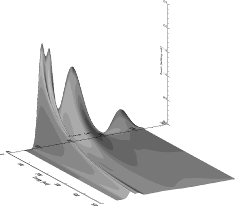
Figure 4: The synthetic 3D model of GRB 090618. Each pulse is generated separately with their respective best-fit parameters. The pulses are then shifted to their respective start time, and co-added to generate the full GRB (Source: Basak & Rao 2012b)

As we have all the required parameters for the 3D pulse description, we regenerate the pulses, shift them to the respective start time, and co-add them to generate the full GRB. For illustration purpose, we have shown the 3D view of GRB 090618 in Figure 4. The four pulses of the GRB are clearly visible. The count is shown (in arbitrary units) as a function of time and energy. The photon spectrum at any instance is a Band function, and the LC in any energy band is a Norris model. Note that this figure is used to display the 3D structure of the pulses up to normalization factors. When we use this 3D model to obtain various pulse parameters, we normalize the pulses and then derive the parameters. However, as pulse width ($w$) is defined as the time interval between the points with 1/e flux values relative to the peak, and spectral lag ($\tau$) is defined as the difference in the peak position of the lightcurve in two energy bands, they do not depend on the normalization.

5 Timing Analysis Using the 3D Model

A 3D pulse model can be used in many ways to derive various pulse properties. In our study, we have done the following analyses.

1 Synthetic Lightcurves

For the best-fit values of $E_{\rm peak,0}$ and $\phi_{0}$, we generate the 3D model of each pulse, and integrate them over some desired energy band ($E_{1}$ to $E_{2}$). This gives LC of each pulse. We shift the LCs to the respective start time to generate the full LC. We choose the same energy bands which we used earlier for Norris model fit to the LCs (section 3.3.1). These are 15-25, 25-50, 50-100, and 100-200 keV.

Figure 5: The synthetic LC of GRB 090618 in 25-50 keV energy band, over-plotted on the BAT LC in the same energy band. Note that, except for the rapid variability, the synthetic LC captures the observed LC quite well (Source: Basak & Rao 2012b).

Figure 6: Left Panel: Variation of $w$ in different energy bands for the four pulses (upper to lower — pulse 1-4) as obtained by using the 3D pulse model. Note that the first two pulses have normal width broadening, while the last two pulses show anomalous width broadening. Right Panel: A comparison between the width ($w$) of the four pulses obtained from directly fitting the LCs (Norris model fit), and those obtained from the synthetic pulse LCs. The dot-dashed line is the line of equality. (Source: Basak & Rao 2012b).

In Figure 5, we have shown the synthetic LC in 25-50 keV energy band, over-plotted with the BAT LC in the same energies. The count rate is the BAT mask weighted count rate. Note that the LC has rapid time variability superimposed on the the broad pulse structure. In our pulse description, we consider only the smooth and broad time variability. The rapid variability timescales generally give large $\chi^{2}$ when we use the smooth synthetic LC for fitting. Hence, the normalization factors cannot be determined by using $\chi^{2}$ minimization technique. Instead, we estimate the factors by physically inspecting the LCs. It is worthwhile to mention again that due to the large overlap, the first two pulses have been considered as a single entity. Hence, the derived model parameters ($E_{\rm peak,0}$ and $\phi_{0}$) are average quantities. This averaging effect essentially shows up in the derived LC. However, note that except for the rapid variability, the synthetic LC is in good agreement with the data. Hence, we conclude that the assumption of $E_{\rm peak}$ evolution (equation 3), along with the the global parameters of our model correctly reproduce the energy-resolved LCs. This finding also validates the fact that each pulse can be considered as a HTS pulse. The IT behaviour is possibly a superposition effect.

2 Deriving The Timing Parameters

Using the synthetic light curves in different energy bands, one can derive various parameters characterizing a pulse. We shall derive the following pulse properties — pulse width ($w$), and spectral lag ($\tau$). The derived parameters, and their energy evolution will be checked with the values as derived from the direct observation. We can derive the pulse width of the individual pulses by directly fitting the LCs (equation 1), and then using the best-fit model parameters ($\tau_{1}$, $\tau_{2}$) as done in section 3.3.1. The spectral lag ($\tau$) between two energy bands can be calculated by cross-correlating the LCs in those energy bands (Rao et al. 2011). Note that due to the overlapping effect, the direct measurement of $w$ and $\tau$ can be erroneous. This effect will be less severe for the $w$ measurement. Of course, the rising part of a pulse can be affected by the falling part of the preceding pulse, broadening the width. But, the fact that all the pulses are simultaneously fitted with Norris model, takes care of the overlapping effect. However, $\tau$ would be affected by the overlapping effect in a similar way as two overlapping HTS pulses leads to a IT (or rather soft-to-hard-to-soft — SHS) behaviour in the overlapping region. In these cases, the 3D pulse model is very useful. As the pulses are independently generated, the derived $w$ and $\tau$ will be unaffected by the overlapping effect.

Table 3: Pulse width ($w$) variation of the four pulses with the energy bands. The numbers in parentheses are $w$ measured by the Norris model fit

Pulse	15-25 keV	25-50 keV	50-100 keV	100-200 keV
1	$6.05_{-0.12}^{+0.12}$	$5.88_{-0.16}^{+0.16}$	$5.54_{-0.17}^{+0.16}$	$5.08_{-0.18}^{+0.15}$
	($6.74_{-0.13}^{+0.13}$)	($6.67_{-0.39}^{+0.39}$)	($6.18_{-1.62}^{+1.62}$)	($5.79_{-0.30}^{+0.30}$)
2	$6.56_{-0.19}^{+0.22}$	$6.35_{-0.19}^{+0.22}$	$5.89_{-0.34}^{+0.27}$	$5.33_{-0.34}^{+0.20}$
	($7.52_{-0.13}^{+0.13}$)	($7.40_{-0.04}^{+0.04}$)	($7.23_{-0.11}^{+0.11}$)	($6.82_{-0.04}^{+0.04}$)
3	$17.84_{-0.70}^{+0.47}$	$18.10_{-0.89}^{+0.53}$	$18.68_{-0.96}^{+0.74}$	$19.82_{-0.64}^{+0.49}$
	($18.01_{-3.91}^{+3.91}$)	($18.09_{-0.40}^{+0.40}$)	($17.22_{-1.43}^{+1.43}$)	($15.87_{-1.63}^{+1.63}$)
4	$14.45_{-0.92}^{+0.99}$	$14.66_{-0.96}^{+0.98}$	$15.18_{-0.88}^{+0.62}$	$15.93_{-1.27}^{+1.16}$
	($13.32_{-0.51}^{+0.51}$)	($13.76_{-1.60}^{+1.60}$)	($14.00_{-1.23}^{+1.23}$)	($13.03_{-1.84}^{+1.84}$)

A. Pulse Width Variation With Energy

We generate the LCs in various energy bands, measure the peak position, and calculate the width at the two points where intensity is $\rm exp(-1)$ factor of the peak intensity. This is essentially the same definition used for $w$ calculation using Norris exponential model. We define $\tau$ of an energy band as the peak position of the LC with respect to that of the lowest energy band (15-25 keV). Note that our model assumes global values of certain parameters ($\tau_{1}$, $\tau_{2}$, $\alpha$ and $\beta$) characterized by the pulse-averaged values. The $E_{peak}(t)$ is the only time variable parameter which depends on LK96 model parameters — $E_{peak,0}$, $\phi_{0}$. Hence, all the timing properties of a pulse (i.e., $w$ and $\tau$ at various energy bands) are essentially determined by the evolution law of $E_{peak}(t)$.

In Table 3 and 4, we have shown the $w$ and $\tau$ as derived from the synthetic LCs of the pulses. In Table 3, the numbers shown in parentheses are those obtained by directly fitting the pulse LCs with Norris model. In Figure 6 (left panel), we compare $w$ as derived from these very different methods. We note that the observations and predictions match quite well. From Table 3, we notice for the first two pulses that $w$, as derived by our model have systematically lower values than the directly measured values. This is due to the fact that these two pulses are considered together in our model. But, as we have developed the 3D model of these pulses separately, we believe that the derived widths are devoid of overlapping effect. A complete disentanglement of heavily overlapping pulses can give more secured values, however, it is difficult to achieve in our model.

Figure 7: A comparison of the slopes of linear fit to the $E-w$ data as found by directly fitting the data with Norris model, and by using our 3D pulse model (Source: Basak & Rao 2012b).

We now study the variation of $w$ with energy. As discussed in section 3.3.1 pulse widths are expected to be broader at lower energies (Norris et al. 1996, Hakkila & Preece 2011). We call this normal width broadening. However, as already pointed out (Figure 2), we also have anomalous width broadening (i.e., width decreases with decreasing energy at lower energy bands) for the last two pulses. In Figure 6 (left panel), we have shown the variation of $w$ as a function of energy for the four pulses. It is clear that the first two pulses follow the normal trend, while the last two pulses have a reverse $E-w$ variation. This reverse variation cannot arise from any contamination effect as could have been an argument for direct LC fitting. For the individual pulses, we fit the $E-w$ data with linear function. We obtain $(-9.4\pm 1.7)\times 10^{-3}$ s $\rm keV^{-1}$, and $(-11.8\pm 2.4)\times 10^{-3}$ s $\rm keV^{-1}$ for the first two pulses with $\chi^{2}$ (dof) = 0.13 (2) and 0.11 (2), respectively. These slopes are convincingly negative. However, the $E-w$ slope of the last pulses are positive ($(18.8\pm 11.1)\times 10^{-3}$ s $\rm keV^{-1}$, and $(14.2\pm 10.6)\times 10^{-3}$ s $\rm keV^{-1}$ with $\chi^{2}$ (dof) = 0.0046 (2) and 0.0021 (2), respectively). Note that the errors in the $E-w$ slope has improved from our previous study of LC with direct Norris model fit. The improvement is apparent for the third pulse ($(18.8\pm 11.1)\times 10^{-3}$ s $\rm keV^{-1}$ compared to $(15\pm 14)\times 10^{-3}$ s $\rm keV^{-1}$). Hence, at least for this pulse the evidence of anomalous width broadening is convincing. In the right panel of Figure 6, we have compared the values of $w$ as obtained by the new pulse model and Norris model fitting. We note that the derived values are similar to each other. In Figure 7, we have compared the slope of the $E-w$ data of the four pulses as obtained from the two methods. We again note a general agreement between the data.

Figure 8: The normal and anomalous width broadening region as found by the ratio plot of $w_{4}/w_{1}$ as a function of $\tau_{1}$. The two regions are separated by the equality line $w_{4}/w_{1}=1$. Different curves are obtained for different values of $\tau_{2}$, which are varied in the range (0.54 to 2.47) from 0.54 (right most), 1.20, 1.90 and 2.47 (left most). The values of $\tau_{1}$ for the first and thirst pulse (795.4 and 353.4, respectively) are shown by dot-dashed line. For example, the set of values for pulse 1 ($\tau_{1}=795.4$, $\tau_{2}=0.54$) is covered by the right most curve, and it falls in normal width broadening region (Source: Basak & Rao 2012b).

Table 4: The model predicted spectral delay of higher energy photons with respect to the photons in 15-25 keV energy band (mean energy = 20.82 keV). Values are calculated for the individual pulses

Pulse	Energy Channel	Mean Energy (keV)	Delay (s)
1	15-25 vs. 25-50 keV	35.45	$-0.135_{-0.022}^{+0.011}$
	15-25 vs. 50-100 keV	68.07	$-0.375_{-0.039}^{+0.023}$
	15-25 vs. 100-200 keV	123.73	$-0.730_{-0.045}^{+0.043}$
2	15-25 vs. 25-50 keV	35.45	$-0.195_{-0.005}^{+0.005}$
	15-25 vs. 50-100 keV	68.07	$-0.555_{-0.033}^{+0.033}$
	15-25 vs. 100-200 keV	123.73	$-1.070_{-0.037}^{+0.023}$
3	15-25 vs. 25-50 keV	35.45	$-0.015_{0.040}^{+0.041}$
	15-25 vs. 50-100 keV	68.07	$-0.040_{-0.030}^{+0.012}$
	15-25 vs. 100-200 keV	123.73	$-0.085_{-0.005}^{+0.005}$
4	15-25 vs. 25-50 keV	35.45	$-0.020_{-0.010}^{+0.010}$
	15-25 vs. 50-100 keV	68.07	$-0.065_{-0.040}^{+0.035}$
	15-25 vs. 100-200 keV	123.73	$-0.095_{-0.005}^{+0.005}$

The anomalous width broadening as observed for the last two pulses, may have a direct physical reason. However, in our analysis, we have used only empirical models for a pulse description. Hence, we shall try to give a phenomenological reasoning for reverse width variation. Our motivation for such study is to show that a reverse width variation can indeed occur due to a particular combination of model parameters instead of a sensitivity limit of the detector at the lower energy band. First, we consider pulse 1 and pulse 3, which are the two most convincing cases of normal and anomalous width variation, respectively. From Table 2, let us compare their parameters. In the parentheses, we have shown the values for pulse 3. These are (in usual units): LK96 parameters — $E_{peak,0}=359~{}(324)$, $\phi_{0}=12.2~{}(18.8)$, pulse-average photon indices — $\alpha=-1.11~{}(-1.15)$, $\beta=-2.5~{}(-2.5)$, and time constants of Norris model — $\tau_{1}=795.4~{}(353.4)$, $\tau_{2}=0.54~{}(2.47)$. It is evident that the two pulses have all the parameters nearly similar, except for $\tau_{1}$ and $\tau_{2}$. Hence, these two global parameters are the main contributors for the difference in $E-w$ relation of these two pulses. To test how these parameters affect the width variation, let us explore the parameter space of $\tau_{1}$ and $\tau_{2}$ with all other parameters fixed to the values of the first pulse. Let us define broadening as the ratio of width in 100-200 keV band ($w_{4}$) to that in 15-25 keV band ($w_{1}$). We say that a pulse follows a normal broadening law if $\frac{w_{4}}{w_{1}}>1$, and anomalous, otherwise. The procedure is as follows. We shall assume a few values of $\tau_{2}$ in the range $0.54-2.47$ (the values of $\tau_{2}$ for pulse 1 and 3, respectively), and vary $\tau_{1}$. This is because $\tau_{2}$ has a relatively small range. For these values of $\tau_{2}$, we shall essentially generate many synthetic LCs with a range of $\tau_{1}$. For each realization, we calculate $\frac{w_{4}}{w_{1}}$. A plot of $\frac{w_{4}}{w_{1}}$ with $\tau_{1}$ for a particular value of $\tau_{2}$ gives the region of normal and anomalous width broadening characterized by $\tau_{2}$.

In Figure 8, we have shown the regions of parameter space where a normal and anomalous width broadening can occur. The whole plot is divided into two regions by $w_{4}$/$w_{1}=1$ line — (i) $w_{4}<w_{1}$ (lower region), and (ii) $w_{4}>w_{1}$ (upper region) for which we get a normal and anomalous broadening, respectively. Different curves represent different values of $\tau_{2}$, from right to left 0.54, 1.20, 1.90 and 2.47. For a given value of $\tau_{2}$, a pulse tends to show anomalous broadening for higher values of $\tau_{1}$. Also, the lower the value of $\tau_{2}$, the higher the allowed value of $\tau_{1}$ for a normal width broadening. The set of values for the first pulse ($\tau_{1}=795.4$, $\tau_{2}=0.54$) is securely positioned in the normal broadening region of the right most curve. The values of the third pulse ($\tau_{1}=353.4$, $\tau_{2}=2.47$) marginally appears in the anomalous region of the left most curve. Hence, the third pulse is likely to show a reverse width broadening. Note that the parameters used for the third pulse are those of the first pulse, except for the values of $\tau_{1}$ and $\tau_{2}$. Still we get anomalous broadening for this pulse. This shows that the combination of $\tau_{1}$ and $\tau_{2}$ of this pulse is prone to the reverse width variation. It also signifies that the $E-w$ data is really insensitive to the other parameters.

B. Spectral Lag of Different Energy Bands

We now study the spectral lag of different energy bands with respect to the lowest energy band (15-25 keV). As we have assumed a HTS evolution in each of the pulses, we expect the soft x-rays to lag behind the hard x-rays. In Figure 9, we have shown the spectral lag of the four pulses in three different energy bands. It is clear that the lags are negative, showing the soft delay. The model predicted spectral delay can be compared with the observed delay (Rao et al. 2011). These are shown in Figure 10 . The time bins used by Rao et al. (2011) are $0-50$ s, $50-77$ s, $77-100$ s $100-180$ s (post-trigger). The first bin is the precursor, hence neglected for the lag calculation. In the second time bin, pulse 1 and 2 appear together. The third bin captures the third pulse, while we neglect the fourth bin owing to the large difference of time cut. In Figure 10, we have shown the data of pulse 1 and 2 both for a single delay quoted for the second time interval, $50-77$ (the lowest 6 data points, with left points for pulse 2). We note that the data in general agrees with the model predicted delay, though with a deviation for the first pulse. This is, of course, due to the fact that the two pulses are combined for the calculation of the observed delay. Note that the second pulse is closer to the observed value. Another important point is that we can find the spectral lag even within the overlapping pulses by the simultaneous timing and spectral description. Also, one has to consider the fact that we are using only the peak position rather than performing a cross-correlation as was done by Rao et al. (2011).

3 Summary Of 3D Pulse Description

Before going to the next section, let me summarize the essential points that we have discussed. We have attempted to describe the individual pulses of a GRB simultaneously in time and energy domain. Our main assumptions are (i) $E_{\rm peak}$ has a HTS evolution (equation 3) within a pulse, (ii) an instantaneous spectrum can be described by Band function (equation 2) with the spectral indices represented by the pulse-average value, and $E_{\rm peak}(t)$ is given by equation 3, and (iii) the pulse LC has a Norris model shape with the time constants determined by the average values. With these simple assumptions, we have developed a table model in XSPEC to derive the model parameters. We have successfully generated the model with best-fit parameters, and derived various pulse properties (LC, width, lag), and matched with the data. We found a tentative evidence of an anomalous width broadening in the data, which is phenomenologically explained by a combination of model parameters.

One of the most important applications of the pulse-wise description is that it can be used for GRBs with multiple pulses. As these pulses can be generated separately, the parameters have little overlapping effect. In the next section, we shall apply this model for a set of GRBs, most of which have multiple pulses.

Figure 9: The model predicted spectral lag for the four pulses (squares, circles, stars and triangle, respectively) are shown. The values are calculated using 15-25 keV as the reference band. Hence, a negative value denotes a soft lag. In fact soft lag is expected due to the assumption of HTS evolution (Source: Basak & Rao 2012b).

Figure 10: A comparison between the spectral lag derived from the new model, and the observed lag calculated by cross correlation (Rao et al. 2011). the dot-dashed line shows the equality. The lower 6 data points are model predicted lag for pulse 1 (the ones in the right) and pulse 2 (the ones in the left), as compared to the 50-77 s data of Rao et al. (2011, see text). Source: Basak & Rao (2012b).

6 A New Pulse-wise GRB Correlation

Aided with a simultaneous timing and spectral description of the individual pulses of a GRB, we now apply this model on a set of GRBs (Basak & Rao 2012a). In this section, we shall study Amati correlation (Amati et al. 2002), which essentially says that a GRB with high peak energy ($E_{\rm peak}$) has high isotropic energy ($E_{\gamma,\rm iso}$). This statement can be reverted as — a GRB with high energy ($E_{\gamma,\rm iso}$) produces higher energy photons. The physical reason of this correlation is unknown, but Amati et al. (2002), using 9 BATSE GRBs found a significant correlation (Spearman rank, $\rho=0.92$, corresponding to a chance probability, $P_{\rho}=5.0\times 10^{-4}$). In the source frame this correlation is approximately $E_{\rm peak}\sim E_{\gamma,\rm iso}^{0.52\pm 0.06}$. With a larger set of GRBs (41), Amati (2006) have shown that the correlation still holds ($\rho=0.89$, $P_{\rho}=7.0\times 10^{-15}$). Similar correlation between $E_{\rm peak}$ and isotropic luminosity ($L_{\rm iso}$) was later found by Yonetoku et al. (2004) for a set of 16 GRBs (Pearson correlation, $r=0.958$, $P_{\rm r}=5.31\times 10^{-9}$). Ghirlanda et al. (2004a), on the other hand, replaced $E_{\gamma,\rm iso}$ by the collimation corrected energy ($E_{\gamma}$) and found reasonable correlation for 27 GRBs ($\rho=0.80$, and $P_{\rho}=7.6\times 10^{-7}$). For a selected sample of 24 GRBs, this correlation improves ($\rho=0.88$).

However, all these correlations are empirical, and can as well arise due to the selection bias of the instrument (Band & Preece 2005, Nakar & Piran 2005, Schaefer & Collazzi 2007, Collazzi et al. 2012). One way to argue against the selection bias is to prove a correlation within the time-resolved data. For example, Ghirlanda et al. (2010b) have studied 9 GRBs with known $z$. They have studied time-resolved $E_{\rm peak}-L_{\rm iso}$ correlation, and established its reliability. In this regard, it is important to check the time-resolved Amati correlation. Hence, we take the sample used by Ghirlanda et al. (2010b) and study the Amati correlation.

In the following analysis, a $\Lambda$-CDM cosmology is assumed. Hence, we use the following parameters of cosmology. The Hubble parameter, $H_{\rm 0}=\rm 71~{}km~{}s^{-1}~{}Mpc^{-1}$, the dark energy density, $\Omega_{\rm\Lambda}=0.73$, total density of baryonic and dark matter, $\Omega_{\rm m}=0.27$, and a spatially flat universe. The values used here are determined by combining 7-year data of Wilkinson Microwave Anisotropy Probe (WMAP; Jarosik et al. 2011), data from Baryon Acoustic Oscillations (Percival et al. 2010), and the data from Type Ia supernova observation (Riess et al. 2011). The recent measurements done by Planck mission indicates slightly different values of the parameters, namely, $H_{\rm 0}=\rm 67.3~{}km~{}s^{-1}~{}Mpc^{-1}$, $\Omega_{\rm m}=0.315$ (Planck Collaboration et al. 2013). The new values primarily alters the values of $E_{\rm\gamma,iso}$ at low $z$, e.g., at $z=1$, 3 and 10, the changes are $\approx$ 7.0%, 3.6% and 1.7%. As the $E_{\rm peak}$ values remain unaltered, the slope and normalization of the relations will slightly change.

1 Time-integrated, Time-resolved And Pulse-wise Amati Correlation

We use the sample of Ghirlanda et al. (2010b) for our correlation study. They have selected GRBs detected by the Fermi/GBM, and having secured redshift ($z$) measurement. A Swift/BAT sample can provide a larger set. However, due to a limited energy coverage (15-150 keV), the Swift/BAT often cannot give reliable value of $E_{\rm peak}$. A joint Fermi/GBM-Swift/BAT analysis gives $\sim 10\%$ higher $E_{\rm peak}$ (chapter 2). For this reason, we shall also re-analyze the Fermi/GBM data of GRB 090618. To remind, the Swift/BAT data of this GRB was used to demonstrate the 3D pulse model. The original Ghirlanda et al. (2010b) sample contains 12 GRBs. Among these three GRBs (GRB 080905, GRB 080928, and GRB 081007) have very low flux. Ghirlanda et al. (2010b) could fit only a single power-law with unconstrained peak energy for these bursts. Hence, these bursts are not suitable for a detailed time-resolved study. Hence, we are left with 9 GRBs (after sample selection). In Figure 11, we have shown the time-integrated data of the 9 GRBs by filled boxes. We obtain a reasonable correlation (Pearson, $r=0.80$, with $P_{\rm r}=0.0096$). For the time-resolved study, we use the same bins of Ghirlanda et al. (2010b). When we study the time-resolved data, we see the correlation is poor (small circles in Figure 11). The correlation coefficient is only $r=0.37$, with $P_{\rm r}=0.0095$. The reason that this correlation is poor can be attributed to the HTS evolution of the pulses. As a HTS evolution, by definition, has high $E_{\rm peak}$ values even when the flux is low, it fills the upper left region of the Amati correlation (see Figure 11).

Table 5: The isotropic energy ($E_{\gamma,\rm iso}$), observer frame values of peak energy ($E_{peak}$) and peak energy at zero fluence ($E_{\rm peak,0}$) are shown for the pulses of GRBs with known redshift ($z$). The GRBs are taken from Ghirlanda et al. (2010b).

GRB	z	Pulse	$t_{1}$	$t_{2}$	$E_{peak}$	$\chi_{red}^{2}$	$E_{peak,0}$	$\chi_{red}^{2}$	$E_{\gamma,iso}$
			(s)	(s)	(keV)		(keV)		($10^{52}$erg)
080810	3.35	1	20.0	28.0	$354_{-61}^{+188}$	0.95	$875_{-180}^{+155}$	0.99	7.7
080916C	4.35	1	0.0	13.0	$430_{-67}^{+87}$	1.17	$2420_{-397}^{+523}$	1.21	158.9
		2	16.0	43.0	$477_{-82}^{+108}$	1.11	$1575_{-150}^{+170}$	1.38	130.1
080916	0.689	1	-1.0	10.0	$155_{-19}^{+23}$	1.12	$519_{-59}^{+44}$	1.36	0.78
		2	13.0	25.0	$70_{-9}^{+13}$	1.0	$226_{-28}^{+285}$	1.00	0.25
		3	28.0	39.0	$39.7_{-7}^{+9}$	1.09	$70_{-23}^{+12}$	1.10	0.05
081222	2.77	1	-2.0	20.0	$159_{-17}^{+22}$	1.42	$488_{-156}^{+173}$	1.07	23.7
090323	3.57	1	-2.0	30.0	$697_{-51}^{+51}$	1.33	$2247_{-298}^{+392}$	1.46	127.9
		2	59.0	74.0	$476_{-47}^{+57}$	1.38	$1600_{-94}^{+35}$	1.95	90.3
		3	137.0	150.0	$117_{-28}^{+31}$	1.37	$211_{-63}^{+54}$	1.17	20.9
090328	0.736	1	3.0	9.0	$648_{-124}^{170}$	0.93	$1234_{-146}^{+174}$	0.92	2.8
		2	9.0	20.0	$659_{-106}^{+115}$	1.25	$1726_{-122}^{+221}$	1.41	4.4
		3	55.0	68.0	$89_{-20}^{+41}$	1.16	$180_{-96}^{+267}$	1.03	0.36
090423	8.2	1	-11.0	13.0	$76.9_{-26}^{+56}$	1.10	$131_{-43}^{+99}$	1.04	20.3
090424	0.544	1	-0.5	3.0	$153_{-5}^{+6}$	1.73	$184.5_{-19}^{+38}$	1.43	2.0
		2	3.0	6.0	$148_{-7}^{+8}$	1.41	$162_{-9.2}^{+61}$	1.32	1.4
		3	6.5	13.0	$39.1_{-8.4}^{+0.2}$	1.32	$104.8_{-16}^{+17}$	1.27	0.18
		4	13.5	20.0	$19.6_{-14.8}^{+6.4}$	0.98	$75_{-34}^{+23}$	0.95	0.10
090618	0.54	1	-1.0	41.0	$185_{-25}^{+26}$	1.24	$415_{-28}^{+37}$	1.19	3.5
		2	61.0	76.0	$226_{-9}^{+10}$	1.25	$382_{-30}^{+106}$	1.33	9.8
		3	76.0	95.0	$128_{-5}^{+6}$	1.15	$218_{-5.8}^{+6.8}$	1.09	5.4
		4	106.0	126.0	$57.7_{-3.3}^{+3.5}$	1.08	$205_{-12}^{+14}$	1.19	1.5

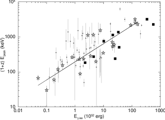
Figure 11: Correlation between the isotropic energy ($E_{\gamma,\rm iso}$) and peak energy ($E_{\rm peak}$) in the source frame, known as the Amati correlation (Amati et al. 2002) is shown. The correlation is studied for time-integrated (filled boxes), time-resolved (smallest circles) and pulse-wise (stars) data. The time-resolved data is obtained by requiring equal integrated flux in each time bin (Ghirlanda et al. 2010b), and it does not consider the broad pulse shape. The linear fit to the pulse-wise data is also shown (Source: Basak & Rao 2012a).

Table 6: Results of the statistical analysis: $E_{\rm peak}$-$E_{\gamma,\rm iso}$(I to IV), and $E_{\rm peak,0}$-$E_{\gamma,\rm iso}$ (V) correlations. Parameters of the linear functional fit to the individual data are also shown.

Method	r	$P_{\rm r}$	K	$\delta$	$\sigma_{int}$	$\chi_{red}^{2}$(dof)
	($\rho$)	($\rm P_{\rho}$)
I	0.80	0.0096	0.166$\pm$0.080	0.473$\pm$0.048	0.225$\pm$0.067	0.64 (7)
	(0.75)	0.0199
II	—	0.004	0.162$\pm$0.085	0.476$\pm$0.079	—	0.47 (8)
III	0.37	0.0095	—	—	—	—
	(0.486)	(0.0003)
IV	0.89	2.95$\times 10^{-8}$	0.289$\pm$0.055	0.516$\pm$0.049	0.244$\pm$0.048	0.56 (20)
	(0.88)	(4.57$\times 10^{-8}$)
V	0.96	1.60$\times 10^{-12}$	0.640$\pm$0.050	0.555$\pm$0.050	0.291$\pm$0.039	1.04 (20)
	(0.87)	(1.43$\times 10^{-7}$)

Notes. Here, the methods are — I: Time-integrated correlation study for 9 GRBs (our work), II: Time-integrated correlation study for 10 GRBs (quoted from Ghirlanda et al. 2010b. Note that they have used 9 GRBs for time-resolved study). III: Time-resolved correlation study (calculated from Ghirlanda et al. 2010b). Time-resolved analysis does not consider broad pulses. IV: Pulse-wise correlation study (our work). V: Pulse-wise $E_{peak,0}$ - $E_{\gamma,iso}$ correlation study. The other parameters are: Pearson correlation coefficient — $r$, Spearman rank correlation coefficient — $\rho$, chance probability — P) (both the correlations), and the best-fit parameters (K, $\delta$ and $\sigma_{int}$).

In order to restore the correlation, we now try pulse-wise analysis. Note that time-resolved analysis does not consider the broad pulses in a GRB. Rather it is guided by the requirement of equal time-integrated flux in a time bin. Hence, we are bound to loosen the correlation. A pulse-wise analysis, on the other hand, takes the broad pulses into account. Hence, it is likely that a pulse-wise analysis is better suited for such a correlation study. We select 22 pulses in these GRBs, and study the pulse-wise correlation. The pulse selection is subjective. Following Fishman & Meegan (1995), we categorized the pulses as (i) single, (ii) smooth, multiple, (iii) separate episodic, and (iv) rapid, or chaotic. In selecting pulses, we neglect the fourth category of pulses/ a portion of a pulse. This way we get clean broad pulses. It is worthwhile to mention that the selected pulses almost always cover the full GRB, except for a few very rapid portions. In Table 5, we have shown the GRB sample, their $z$, and the pulse start and stop times. We neglect some portions of a few bursts, because, either these portions have very low count to be properly used for pulse-wise analysis, or these have rapid variability without any proper pulse structure. GRB 080810 and GRB 080916C have very low count rates after 30 s and 55 s, respectively. GRB 090323 has multiple spiky events in the range $30-59$ s, and $75-135$ s. Also, it has low count rate in $75-135$ s region. GRB 090328 contains two overlapping spiky pulses in the range $20-26$ s (which is divided into two region by Ghirlanda et al. 2010b — $20-24$ s, and $24-26$ s). Except for these few regions, we incorporate essentially all the pulses in our analysis.

We have fitted the spectrum of each pulse with a Band function. The $E_{peak}$ and the $\chi_{red}^{2}$ of these fits are reported in the table. In Figure 11, we have shown the data points of the pulse-wise analysis by stars. In order to obtain the relation between the $E_{peak}$ (both time-integrated and pulse-wise), and $E_{\gamma,\rm iso}$ we apply the following technique. We fit the data by a linear function which can be written as

$$\rm log(\frac{E_{\rm peak}}{100\rm keV})=K+\delta\rm log(\frac{E_{\rm\gamma,iso}}{10^{52}\rm erg})$$ (4)

We also assume an intrinsic data scatter ($\sigma_{\rm int}$) in $E_{peak}$ (D’Agostini 2005). An intrinsic scatter in the dependent variable denotes our limited knowledge of its relation with the independent variable (or, variables). It admits that the dependent variable can be a function of some extra “hidden” parameter (or, parameters), which we are not aware of. This is a general practice in GRB correlation study (e.g., see Ghirlanda et al. 2010b, Wang et al. 2011). With these parameters, we maximize the joint likelihood function ($L$) (Wang et al. 2011) of the form

$$L(K,\delta,\sigma_{\rm int})\propto\prod_{i}\frac{1}{\sqrt{\sigma_{\rm int}^{2}+\sigma_{y_{i}^{2}}+\delta^{2}\sigma_{x_{i}^{2}}}}\\ \times{\rm exp}\left[-\frac{(y_{i}-K-\delta x_{i})^{2}}{2(\sigma_{\rm int}^{2}+\sigma_{y_{i}^{2}}+\delta^{2}\sigma_{x_{i}^{2}})}\right]$$ (5)

Using equation 24 of Wang et al. (2011), we can find the $\chi^{2}$ as $\chi^{2}$=-2ln$L$. In Table 6, we have shown the correlation coefficient, chance probability as well as the best-fit values of the linear fit parameters ($K$, $\delta$). The methods are summarized in the note of this table. Method I and Method II are essentially the time-integrated correlation. Method III is the time-resolved correlation, which we found very poor. Method IV is the pulse-wise Amati correlation as found in our study. We can immediately see a much better correlation compared to the I-III correlations. This correlation has a coefficient of $r=0.89$ with a chance probability, $P=2.95\times 10^{-8}$. The value of $\delta$, which is the power-law of the relation is 0.516$\pm$0.049. Hence, we obtain a similar index as the original Amati correlation ($0.52\pm 0.06$). This relation can be written as follows.

$$\left[\frac{E_{\rm peak,0}}{100\rm keV}\right]=(0.289\pm 0.55)\times\left[\frac{E_{\gamma,\rm iso}}{10^{52}~{}\rm erg}\right]^{(0.516\pm 0.049)}$$ (6)

Another important fact we notice from Table 6 by comparing $\sigma_{\rm int}$ of method I-III with method IV is that the ratio of $\sigma_{\rm int}$ to number of data is reduced. For example, in method I, this ratio is 0.028, while it is 0.011 for method IV.

2 Correlation of $\bf E_{\gamma,\bf\rm iso}$ with $\bf E_{\rm\bf peak,0}$

The pulse-wise correlation not only restores the Amati correlation, it improves the correlation. For example, Krimm et al. (2009) have used a sample of 22 GRBs from Swift and Suzaku satellites to study both time-integrated and pulse-wise Amati correlation. They have obtained a coefficient, $\rho=0.74$, with $P_{\rho}=7.58\times 10^{-5}$ for time-integrated data. The pulse-wise data of 59 pulses shows an improvement $\rho=0.80$, with $P_{\rho}=5.32\times 10^{-14}$. A pulse-wise correlation also suggests that pulses are (possibly) independent entities.

Though a pulse-wise correlation is more meaningful than a time-integrated correlation study, the fact that $E_{\rm peak}$ is still an average quantity demands an alternative parameter to be used for such analysis. We have one such parameter, namely the peak energy at zero fluence ($E_{\rm peak,0}$). As this parameter is a constant for a given pulse, it is more fundamental. Also, it denotes the initial $E_{\rm peak}$ of a burst, and hence, it carries the initial time information rather than pulse-average $E_{\rm peak}$, where the time information is lost due to the averaging. Some GRB correlations are studied by incorporating the time information e.g., $L_{\rm iso}-E_{\rm peak}-T_{0.45}$ correlation (Firmani et al. 2005, 2006, 2007). However, in our analysis, time information is implicit, and hence, requires one less parameter.

For the set of 22 pulses of the 9 GRBs, we generate their 3D pulse models, and determine the $E_{\rm peak,0}$. We now replace the source frame $E_{\rm peak}$ with the source frame $E_{\rm peak,0}$ and study the pulse-wise correlation. In Table 6, we have shown the correlation coefficient (method V). We immediately see an improvement of the correlation ($r=0.96$, $P_{\rm r}=1.60\times 10^{-12}$). The Spearman rank correlation, however, is similar to the pulse-wise Amati correlation ($\rho=0.87$, $P_{\rho}=1.43\times 10^{-7}$; method IV: $\rho=0.88$, $P_{\rho}=4.57\times 10^{-8}$). This is also reflected in the ratio of $\sigma_{\rm int}$ to number of data, which is 0.013 (compare with method IV: 0.011). Hence, we conclude that $E_{\rm peak,0}$-$E_{\gamma,\rm iso}$ correlation is either comparable (for Spearman correlation), or better (for Pearson correlation) than the pulse-wise Amati correlation. However, note that both the correlations are pulse-wise. Hence, we conclude that pulse-wise correlation is better than time-integrated and time-resolved correlation (that does not account for the broad pulses) in a general sense.

In Figure 12, we have shown the correlation. The data is fitted with a straight line to derive the relation, which is

$$\left[\frac{E_{\rm peak,0}}{100\rm keV}\right]=(0.64\pm 0.05)\times\left[\frac{E_{\gamma,\rm iso}}{10^{52}~{}\rm erg}\right]^{(0.56\pm 0.05)}$$ (7)

The dot-dashed lines denote the $3\sigma_{\rm int}$ data scatter. In this figure, we have marked a few GRBs which have highest number of pulses. As the correlation holds within $3\sigma_{\rm int}$ between the individual pulses, this correlation, like the pulse-wise Amati correlation, is also free from selection bias.

Ghirlanda et al. (2004a) have suggested that if GRBs are indeed jetted events, a collimation corrected energy ($E_{\gamma}$) should be better correlated. Though for a set of 27 GRBs they found reasonable correlation ($\rho=0.80$, which improves to $\rho=0.88$, for a selected sample of 24 GRBs), it is only comparable to $E_{\rm peak}-E_{\gamma,\rm iso}$ correlation. A close inspection of Figure 12 reveals that the pulses of a given burst are scattered on the same direction of the correlation line. This may point towards the fact the actual energy is not $E_{\gamma,\rm iso}$, but $E_{\gamma}$. As the collimation correction is different for different burst, but same for all the pulses of a given burst, it is possible that all the pulses of a GRB scatters away in the same direction from the correlation line. Hence, one can expect to have better correlation by the replacement of $E_{\gamma,\rm iso}$ with $E_{\gamma}$. However, in practice, the value of the jet opening angle ($\theta_{j}$) is either impossible to measure, or has large errors (Goldstein et al. 2011). For the available values of $\theta_{j}$ (6 cases), we replace $E_{\gamma,\rm iso}$ by $E_{\gamma}$, and found a reasonable correlation ($r=0.91$). We believe that the parameters $E_{\rm peak,0}$ and $E_{\gamma}$ can give a much improved correlation provided good measurements of $\theta_{j}$ are available.

Figure 12: Correlation between isotropic energy ($E_{\gamma,\rm iso}$) and peak energy at zero fluence ($E_{\rm peak,0}$) in the source frame is shown. Different pulses of three GRBs are marked, and explained in the legend. The solid line shows the linear fit to the data, and the dot-dashed lines denote the 3$\sigma$ data scatter (Source: Basak & Rao 2012a).

Table 7: The additional sample of GRBs with known $z$, detected by the Fermi/GBM. We have reported here the start and stop time of the pulses, the corresponding best-fit parameters for a Band functional fit ($\alpha$, $\beta$, $E_{\rm peak}$), and the isotropic energy, $E_{\rm\gamma,iso}$ (Basak & Rao 2013c).

GRB	z	Pulse	$t_{\rm 1}$	$t_{\rm 2}$	$\alpha$	$\beta$	$E_{\rm peak,obs}$	$\chi_{red}^{2}$	$E_{\rm\gamma,iso}$
			(s)	(s)			(keV)	(dof)	($10^{52}$erg)
090902B	1.822	1	5.0	13.0	$-0.23_{-0.13}^{+0.13}$	$-3.56_{-0.56}^{+0.22}$	$828.9_{-28.7}^{+31.6}$	1.03 (243)	178.24
		2	12.0	18.0	$-0.76_{-0.04}^{+0.07}$	$-3.21_{-0.38}^{+0.23}$	$537.3_{-23.7}^{+23.5}$	1.34 (290)	111.81
		3	18.0	23.0	$-0.76_{-0.03}^{+0.04}$	$-2.44_{-0.11}^{+0.08}$	$285.4_{-17.0}^{+15.6}$	1.34 (275)	62.14
090926A	2.1062	1	0.0	8.0	$-0.55_{-0.02}^{+0.02}$	$-2.44_{-0.05}^{+0.05}$	$332.1_{-9.6}^{+9.7}$	1.59 (492)	116.83
		2	8.0	15.0	$-0.80_{-0.02}^{+0.02}$	$-2.90_{-0.18}^{+0.13}$	$241.3_{-7.3}^{+7.6}$	1.55 (466)	61.15
090926B	1.24	1	12.0	65.0	$0.13_{-0.40}^{+0.45}$	$-10.0$	$73.8_{-6.1}^{+7.7}$	0.65 (42)	2.54
091003A	0.8969	1	13.95	26.24	$-0.953_{-0.06}^{+0.07}$	$-2.38_{-0.51}^{+0.20}$	$299.4_{-41.0}^{+48.2}$	1.10 (293)	6.05
091020	1.71	1	-2.0	15.0	$-1.16_{-0.15}^{+0.22}$	$-2.07_{-0.50}^{+0.24}$	$197.3_{-75.6}^{+115.9}$	1.07 (134)	8.0
091024	1.092	1	-7.94	33.02	$-0.95_{-0.14}^{+0.22}$	$-2.08_{-\infty}^{+0.47}$	$725.0_{-162.8}^{+226.7}$	0.82 (119)	9.10
		2	200.71	249.86	$-0.81_{-0.26}^{+0.40}$	$-9.37$	$112.7_{-14.6}^{+14.4}$	1.43 (81)	3.74
		3	313.35	346.12	$-1.18_{-0.07}^{+0.10}$	$-9.36$	$225.7_{-27.5}^{+19.4}$	1.60 (335)	9.14
		4	622.7	664.7	$-1.17_{-0.07}^{+0.07}$	$-2.15$	$371.0_{-71.0}^{+111.0}$	1.09 (473)	2.45
091127	0.490	1	-2.0	4.0	$-0.92_{-0.16}^{+0.19}$	$-2.20_{-0.14}^{+0.08}$	$65.8_{-9.3}^{+12.1}$	1.35 (151)	1.06
		2	5.0	14.0	$-1.34_{-0.33}^{+0.77}$	$-2.88_{-0.17}^{+0.17}$	$14.6_{-3.5}^{+1.7}$	1.00 (140)	0.44
091208B	1.063	1	-1.0	5.0	$-1.36_{-0.24}^{+1.08}$	$-2.30$	$74.2_{-34.9}^{+41.2}$	1.19 (154)	0.55
		2	6.0	13.0	$-1.25_{-0.13}^{+0.13}$	$-2.84_{-\infty}^{+0.48}$	$113.7_{-15.8}^{+30.8}$	1.19 (223)	1.31
100414A	1.368	1	1.0	13.0	$-0.14_{-0.07}^{+0.08}$	$-4.90_{-\infty}^{+1.47}$	$557.5_{-28.5}^{+31.1}$	1.10 (275)	22.73
		2	14.0	20.0	$-0.56_{-0.06}^{+0.06}$	$-3.52_{-\infty}^{+0.71}$	$599.4_{-44.3}^{+49.7}$	1.01 (238)	14.26
		3	21.0	28.0	$-0.91_{-0.05}^{+0.06}$	$-2.76_{-2.42}^{+0.39}$	$635.1_{-78.3}^{+93.5}$	1.17 (240)	12.00
100814A	1.44	1	-3.0	5.0	$1.04_{-0.50}^{+0.65}$	$-3.00_{-2.55}^{+0.71}$	$168.6_{-22.1}^{+25.8}$	0.92 (176)	2.14
		2	4.0	14.0	$0.84_{-0.36}^{+0.55}$	$-3.43_{-\infty}^{+0.95}$	$133.5_{-16.42}^{+13.8}$	0.79 (130)	2.32

7 Pulse-wise Amati Correlation Revisited

The new correlation based on our 3D pulse description is marginally better, or comparable to the pulse-wise Amati correlation. However, the ratio of intrinsic data scatter to the number of points does not improve. The reason for our limited success is two-fold. (i) The models which are used to develop the 3D pulse model are all empirical. We note that the pulse-wise analysis gives a better result than the time-integrated and time-resolved analysis. This is because pulses are possibly physical (e.g., multiple episodes of central engine activity on a longer time scale). On the other hand, the spectral model, and its evolution used to develop our pulse model is empirical. A more physical model of a pulse may help in identifying the correct parameter/parameters for a correlation study. (ii) We have assumed that the pulses are all HTS, and the IT behaviour is a superposition effect. Of course, we have validated this assumption essentially by reproducing LC, width variation and spectral lag. But, as shown in the next chapter (Basak & Rao 2014), IT behaviour is found even for a few GRBs with single pulses. Hence, our assumption may not be applicable in a global sense. However, we can still use the pulses and study pulse-wise analysis.

In this section, we shall study pulse-wise Amati correlation for a larger set of GRBs. The Ghirlanda et al. (2010b) sample contained all $z$-measured GRBs up to June, 2009. We complement the sample by adding all $z$-measured GRBs detected by the Fermi/GBM during June, 2009 to August, 2010. With these additional GRBs (10) our sample contains a total of 19 GRBs. In Table 7, we show the additional sample. The start and stop time of the 21 pulses are shown. We fit the GBM data with Band function. For GRB 090902B, a Band model is unacceptable. Hence, we fit the pulses of this GRB with Band+PL model (Ryde et al. 2010). The best-fit parameters ($\alpha$, $\beta$ and $E_{\rm peak}$) along with $\chi_{red}^{2}$ (dof), and $E_{\rm\gamma,iso}$ are shown in the same table. In Figure 13, we show the pulse-wise Amati correlation for our complete sample. We find a good correlation ($r=0.86$, $P_{\rm r}=1.50\times 10^{-13}$; $\rho=0.86$, $P_{\rho}=7.47\times 10^{-14}$). A Pearson correlation without using the logarithmic values is $r=0.80$. Due to the larger sample size, the significance has increased i.e., chance probability has decreased (previous value was $P_{\rho}=4.57\times 10^{-8}$). The coefficient of the time-integrated Amati correlation for these GRBs is $r=0.83$ with $P_{\rm r}=1.10\times 10^{-5}$; or, $\rho=0.85$ with $P_{\rho}=4.27\times 10^{-6}$. The logarithmic data is fitted with a linear function as before. The corresponding values are shown in Table 8. Note that the slope is close to $\sim 0.5$, which gives the empirical relation $E_{\rm peak}\propto E_{\gamma,\rm iso}^{1/2}$. The values of $K$, $\delta$, and $\sigma_{\rm int}$ are within $0.36\sigma$, $0.36\sigma$, and $0.25\sigma$ of the previous values. The ratio of $\sigma_{\rm int}$ to the number of data points has decreased (0.006).

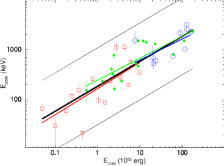
Figure 13: Pulse-wise Amati correlation studied for the 43 pulses of 19 GRBs (Table 5, and 7). The log($E_{\rm peak}$)-log($E_{\rm\gamma,iso}$) data is fitted with a straight line assuming intrinsic data scatter ($\sigma_{\rm int}$), and shown by thick black line. Thin black lines show the $3\sigma_{\rm int}$ data scatter. Markers are: red boxes (z<1), green filled circles (1<z<2), and blue open circles (z>2). Each of these binned data is fitted by a straight line (same colour as the markers), as done for the complete set (Source: Basak & Rao 2013c).

Table 8: Linear fit results for the complete sample is shown. The fitting is performed on the logarithmic values of $E_{peak}$, normalized by 100 keV, and $E_{\gamma,iso}$, normalized by $10^{52}$ erg. The parameters of the linear fit are: intercept ($K$), slope ($\delta$), and intrinsic data scatter ($\sigma_{int}$).

Data set	K	$\delta$	$\sigma_{int}$	$\chi^{2}_{red}$ (dof)
All	$0.269\pm 0.041$	$0.499\pm 0.035$	$0.256\pm 0.0344$	1.04 (41)
z<1 bin	$0.223\pm 0.077$	$0.523\pm 0.113$	$0.306\pm 0.065$	1.13 (15)
1<z<2 bin	$0.391\pm 0.056$	$0.439\pm 0.048$	$0.208\pm 0.047$	1.10 (14)
z>2 bin	$0.373\pm 0.068$	$0.421\pm 0.038$	$0.200\pm 0.063$	1.24 (8)
First/Single pulses	$0.352\pm 0.055$	$0.465\pm 0.044$	$0.221\pm 0.048$	1.10 (17)
Rest of the pulses	$0.228\pm 0.057$	$0.503\pm 0.050$	$0.273\pm 0.048$	1.09 (22)

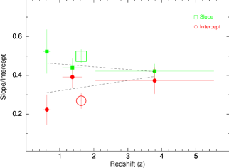
Figure 14: Redshift ($z$) evolution of the pulse-wise Amati correlation is shown. Green filled boxes are the values of slope ($\delta$), and red filled circles are the values of intercept (K) in different redshift bins. The average value of these parameters ($\delta$ and K) are shown by similar open symbols. We fit each of the parameter evolutions with a straight line (Source: Basak & Rao 2013c).

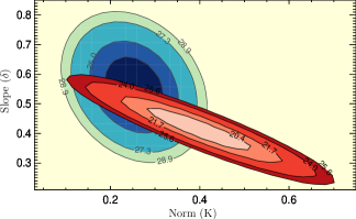
Figure 15: $\chi^{2}$ contour for the parameters $K$ and $\delta$. The parameters are studied in two redshifts — z$\leqslant 1.092$ (shown by blue contours on the left hand side), and z>1.092 (shown by red contours on the right side). In both of the cases, contour levels are — $\Delta\chi^{2}=1.0,2.3,4.61,6.17$ which correspond to 1$\sigma$ (1 parameter), 1$\sigma$, 2$\sigma$, and 3$\sigma$ (2 parameters). We note that the parameters agree within $\Delta\chi^{2}=1.0$ (Source: Basak & Rao 2013c).

1 Redshift Evolution Of The Pulse-wise Amati Correlation

As we have a larger sample compared to the previous study, we can perform some critical tests on the correlation. The first test is to check any possible redshift evolution of the correlation. If we want to use the correlation for cosmology, it is necessary to check the cosmological evolution. For this purpose, we divide our sample into three $z$ bins: (i) $z<1$ (this contains 17 data points), (ii) $1<z<2$ (contains 16 data points), and (iii) $z>2$ (contains 10 data points). In Figure 13, these sets are shown by different markers (red boxes for z<1, green filled circles for 1<z<2, and blue open circles for z>2). Each of the data sets is fitted with a straight line as before. The best-fit values of the linear fits are shown in Table 8. In Figure 14, we have shown these parameters (green filled boxes for $K$, and red filled circles for $\delta$) as a function of the weighted mean $z$ of the corresponding bin. The average values of these parameters are shown by similar open symbols. As we have only three bins, we can at most fit a straight line to quantify the evolution. We find that the evolution of the parameters are consistent with zero. The slopes of the evolution are — $\frac{d\delta}{dz}=(-1.41\pm 3.74)\times 10^{-2}$, and $\frac{dK}{dz}=(2.64\pm 4.88)\times 10^{-2}$. The errors are estimated at nominal 90% confidence level.

The evolution of $K$ and $\delta$ with $z$ is not statistically significant, as the errors are quite large. The evolution of Amati correlation, and other GRB correlation with redshift has been investigated by many authors (e.g., Li 2007, Ghirlanda et al. 2008, Tsutsui et al. 2008, Azzam 2012). In all the study, the evolution is found to be insignificant. Note that the evolution as reported by Tsutsui et al. (2008) is monotonic. But, in our analysis we do not find any such evidence. Rather the evolution saturates at higher $z$ (see high $z$ data points in Figure 14). To further investigate whether their is any significant evolution, we divide the sample into two redshift bins. This way we get larger numbers in each bin though we cannot fit the evolution. As the number of pulses in a given GRB is arbitrary, we cannot get an equal division of sample. The closest we find is 23 pulses in the lower $z$ bin (up to $z=1.096$), and 20 in the higher bin. We fit the individual set of data with straight line, and obtain the parameters. In Figure 15, we have shown the $\chi^{2}$ contour of $K$ and $\delta$. The levels shown are: single parameter $1\sigma$ ($\triangle\chi^{2}=1.0$), two-parameter $1\sigma$ ($\triangle\chi^{2}=2.3$), $2\sigma$ ($\triangle\chi^{2}=4.61$), and $3\sigma$ ($\triangle\chi^{2}=6.17$). We note that the two sets agree within $\triangle\chi^{2}=1.0$. Hence, the evolution is not significant. Yonetoku et al. (2010) have studied the evolution of both Amati and Yonetoku correlation in the time-integrated data. They have found only $1\sigma$ and $2\sigma$ evolution, respectively.

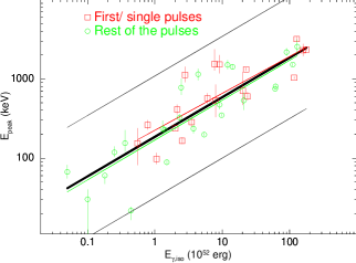
Figure 16: Same as Figure 13, with the set divided into 19 first/single pulses (red open boxes), and 24 rest of the pulses (green open circles). The straight line fitting these sets are shown by the same colour as the markers (Source: Basak & Rao 2013c).

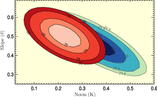
Figure 17: $\chi^{2}$ contours for the parameters $K$ and $\delta$. Contour levels are similar as in Figure 14. Blue contours on the right hand side shows the first/single pulses, while the red contours on the left show the rest of the pulses (Source: Basak & Rao 2013c).

2 Possible Bias For Harder First/Single Pulse

Another possible bias in the pulse-wise correlation can arise from the dependence of spectral hardness of pulses on their time sequence. It is suggested that during the initial phase, GRBs generally tend to be harder than the rest of the prompt emission phase (Crider et al. 1997, Ghirlanda et al. 2003, Kaneko et al. 2003, Ryde & Pe’er 2009). A spectral hardness naturally tends to make higher $E_{\rm peak}$. Hence, it is expected that the first pulse of a GRB should be biased towards higher $E_{\rm peak}$, giving a systematic shift in the pulse-wise correlation.

In order to estimate this bias, we divide our sample in first/single pulses (19 pulses) and the rest of the pulses (24 pulses). We fit the logarithmic values of $E_{\rm peak}-E_{\gamma,\rm iso}$ data by a straight line, and obtained the individual best-fit parameters. In Figure 16, we have shown the two sets of data by red open boxes (first/single pulses) and green open circles (rest of the pulses). The linear fits are shown by the same colours. A comparison with the linear fit to the complete sample (black line) immediately shows that the bias is insignificant. In Table 8, we have reported the fit parameters of these sets. While we see that the intercept ($K$) of the first/single pulse fitting is higher ($0.352\pm 0.055$) than that of the rest of the pulse ($0.228\pm 0.057$), the slope ($\delta$) is lower ($0.465\pm 0.055$ compared to $0.503\pm 0.057$). As the relation between $E_{\rm peak}$ and $E_{\gamma,\rm iso}$ is $E_{\rm peak}\propto 10^{K}E_{\gamma,\rm iso}^{\delta}$, the bias due to higher intercept is compensated by the lower slope.

To further investigate the matter, we plot the $\chi^{2}$ contour of the two sets as before. In Figure 17, the contours are shown. The blue contours on the right side denote the parameter range for the first/single pulse data fitting. The red contours on the left side are those for the rest of the pulses. Again we see that the parameters agree within $\triangle\chi^{2}=1.0$. Hence, we conclude that the bias due to harder first/single pulse is not statistically significant for a pulse-wise Amati correlation.

3 Comparison With The Time-integrated Correlation

It is interesting to compare the pulse-wise Amati correlation with a time-integrated Amati correlation. For this purpose, let us use the recent updated Amati correlation as studied by Nava et al. (2012). Let us denote the values quoted by Nava et al. (2012) by subscript ‘1’. For a complete sample of 46 GRBs, they have reported the a correlation coefficient, $\rho_{1}=0.76$. The slope is found to be $\delta_{1}=0.61\pm 0.04$, while the intercept is $K_{1}=-29.60\pm 2.23$, and $\sigma_{int}=0.25$. They have also studied a larger complementary sample of 90 GRBs with $\rho_{1}=0.78$, $\delta_{1}=0.531\pm 0.02$, $K_{1}=-25.63\pm 1.35$, $\sigma_{int}=0.25$. Together the set contains 136 GRBs with $\rho_{1}=0.77$, $\delta_{1}=0.55\pm 0.02$, $K_{1}=-26.74\pm 1.13$, $\sigma_{int}=0.23$.

In Figure 18, we have shown the time-integrated Amati correlation line of the complete sample (Nava et al. 2012) by red dashed line. The shaded region is the 3$\sigma_{int}$ data scatter of the correlation. In the same figure, we have shown the data points obtained for our pulse-wise analysis (blue filled circles). We have over-plotted the time-integrated data (taken from David Gruber — private communication) of our sample (marked by open circles). The linear fit to the time-integrated data is shown by a dot-dashed line. For comparison, we have also shown the line fitted to the pulse-wise data (thick black line). In our analysis, $E_{\rm peak}$ is normalized by 100 keV, while $E_{\rm\gamma,iso}$ is normalized by $10^{52}$ erg. Hence, in order to compare the best-fit parameters we convert these values in the same units of Nava et al. (2012). We obtain $K=-23.68\pm 1.82$. This value is comparable to the values obtained for the total sample ($K_{1}=-26.74\pm 1.13$). The values of $\delta$ are also comparable ($0.499\pm 0.035$ for pulse-wise analysis, and $0.55\pm 0.02$ for time-integrated analysis of the total sample). Figure 18 clearly shows that all these correlations are comparable within $3\sigma_{\rm int}$ data scatter. A closer look at the plot reveals that the time-integrated correlation line of our sample always lies lower than the pulse-wise correlation line. Hence, the slopes are similar, but the normalization (i.e., the intercepts) of the correlations are different. The difference can be explained as follows. If a GRB with two identical pulse (i.e., same energy and $E_{\rm peak}$) are summed, their total energy will be added up, while the $E_{\rm peak}$ remains the same. Similarly, for pulses with different energies and $E_{\rm peak}$, the resultant total energy will add-up, while the $E_{\rm peak}$ is only an average of them. Hence, we expect a lower normalization for a time-integrated correlation. Note that the correlation coefficient of pulse-wise analysis is always better than the time-integrated analysis.

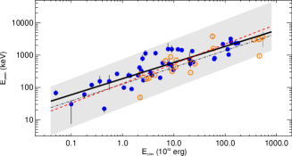
Figure 18: Data set of the complete sample of our study (blue filled circle) as plotted on the plane of time-integrated $E_{\rm peak}$-$E_{\rm\gamma,iso}$ correlation (for the complete sample from Nava et al. 2012). The data for the time-integrated study of 19 GRBs (present analysis) are also shown (orange open circle). The straight line fitted to the pulse-wise log($E_{\rm peak}$)-log($E_{\rm\gamma,iso}$) data is shown by thick black line. The red dashed line denotes the relation between time-integrated $E_{\rm peak}$ with $E_{\rm\gamma,iso}$ (Nava et al. 2012). The blue dot-dashed line shows the similar relation in this study (Source: Basak & Rao 2013c).

8 Summary

In this chapter, we have developed a simultaneous timing and spectral description ($F(t,E)$) of a GRB pulse. Using the synthetic 3D pulse, we have derived various pulse properties and have found consistent results with the data. The agreement between the model and the data extends even to the minute details of the parameters e.g., reverse width variation in some pulses. Such a finding explicitly shows the immense applicability provided by simple assumptions of spectral evolution, even if they are empirical.

We have applied the model to a set of GRBs with known $z$ and found that one of the spectral parameters ($E_{\rm peak,0}$) correlates with the isotropic energy ($E_{\gamma,\rm iso}$) of the pulse. We have found that this correlation is marginally better, or comparable with a pulse-wise $E_{\rm peak}-E_{\gamma,\rm iso}$ correlation. Also, these pulse-wise correlations are always better than time-integrated, or time-resolved (not accounting for broad pulses) correlation. The pulse-wise analysis seems to be more physical, and it is more useful as it favours the reliability of the correlation. Note that the ultimate aim of GRB correlation study is to find luminosity distance e.g., measuring the redshift by an independent way. Using the pulses for such study is quite useful. The pulses, despite having different $E_{\rm peak}$ and $E_{\gamma,\rm iso}$, have the same redshift, and follow the same pulse-wise correlation. Hence, a redshift measured by multiple pulses using the pulse-wise correlation should give a better constraint.

In spite of these versatile applicability, the pulse model is limited by the assumption of spectral model, and its evolution. The assumption of broad pulses seems to be reasonable, as we always get better correlation. Also, the lag-luminosity correlation is found to be a pulse property (Hakkila et al. 2008). However, the other assumptions e.g., instantaneous spectrum is a Band function, and the spectral evolution is always HTS should be critically checked. In the next chapters, we shall scrutinize these assumptions, and explore various other options. We shall find that indeed the assumptions are not valid in a global sense (In fact, there is no physical reason to expect these to be global properties). However, the model is still useful as an empirical description of GRB pulses. Moreover, the pulse model developed here is quite generic in a sense that any empirical timing and spectral function, and spectral evolution can be incorporated, and checked against the data. This is the first attempt to describe GRB pulses in a different approach, and predict various pulse properties from a single description (Basak & Rao 2012b). We again emphasize that a simultaneous description has an immense flexibility to check the validity of a model against the data from various directions.

Chapter 4 Alternative Spectral Models of GRB Pulses

1 Motivation

In this chapter (Basak & Rao 2014), we shall explore various prompt emission models, and compare them with the Band function. The motivation to look for alternative models in the first place is described below. However, note that the Band function till date is the most appropriate function to describe both the time-integrated and time-resolved prompt emission spectrum of GRBs (e.g., Kaneko et al. 2006, Nava et al. 2011, Zhang et al. 2011). Hence, it is unlikely that we shall get any order of magnitude improvement in the spectral fitting. In fact, the alternative models in many cases will be just comparable to the Band function. Also, we do not expect all the GRBs to show any immediate improvement, simply because the data may be flux limited. Hence, we shall apply these models on a selected sample.

• (i) The main reason to study alternative spectral models is to understand the radiation mechanism. Though the Band function is undoubtedly an acceptable function, the physical origin of this function is still debated. In the internal shock model (Rees & Meszaros 1994), the prompt emission is produced via synchrotron radiation of electrons accelerated by “internal shock” in an optically thin region ($r_{\rm IS}\sim 3\times 10^{13}$ cm $\gg r_{\rm ph}\sim 10^{11}$ cm). In certain circumstances, the spectrum can have a synchrotron self-compton (SSC) component, but at a fairly higher energy ($\sim 10$ MeV; section 1.5.2; Sari et al. 1996). Hence, a Band function, in principle, can be a phenomenological representation of an optically thin synchrotron emission. As discussed in section 1.5.2, the electrons emitting synchrotron radiation are expected to cool fast ($\gamma_{\rm e,c}<\gamma_{\rm e,min}$; Piran 1999). Hence, the spectral index is expected to be $-\frac{1}{2}$ (Cohen et al. 1997), i.e., a photon index, $\alpha=-\frac{3}{2}$. Even if the electrons are cooling slowly, the $\alpha$ is expected to be at most $-\frac{2}{3}$. These two limits are referred to as “synchrotron lines of death”. A GRB photon index cannot be greater than -3/2 (or, -2/3, for slow cooling). However, the value of $\alpha$ is found to be greater than -2/3 in many cases (Crider et al. 1997, 1999, Preece et al. 1998). In addition, the synchrotron radiation is supposed to be produced by electrons accelerated in IS. As IS requires interactions of relativistic shells with low relative velocity, the efficiency of energy conversion is low ($\lesssim 20\%$; Piran 1999). Hence, both the IS model and synchrotron emission are inadequate to fully explain the spectrum.

• (ii) It is possible that Band is actually an average function which is produced by the evolution of a different, more physical function (Ghirlanda et al. 2003, Ryde 2004, 2005, Ryde & Pe’er 2009, Pe’er & Ryde 2011). For example, Ryde (2004) has shown that the instantaneous spectrum of the BATSE GRBs with single pulses can be modelled by a blackbody (BB), or a BB along with a power-law (PL). Note that while Band function has a single non-thermal spectral shape, a BBPL model segregates the spectrum into a thermal and a non-thermal component. In a BBPL model, the $\nu F_{\nu}$ peak of the spectrum is represented by the peak of the photospheric temperature as seen by an observer ($\sim 3kT$). Also, as the PL index becomes shallower than $\alpha$ of the Band function, it can be accommodated in the synchrotron interpretation. In a few Fermi GRBs, this PL appears to have a second slope, or a cut-off at high energies. This non-thermal component is modelled with either a cut-off PL (e.g., Ackermann et al. 2011), or a Band function (Guiriec et al. 2011, Axelsson et al. 2012, Guiriec et al. 2013). In one case (GRB 090902B), the time-resolved spectrum is interpreted as a multicolour BB with a PL (mBBPL; Ryde et al. 2010), where mBB represents a departure from the BB shape due to dissipative processes inside the photosphere, and a geometric broadening due to the finite size of the photosphere (Pe’er 2008).

• (iii) The Band function was actually derived by an extensive study of the CGRO/BATSE data in a limited band width. Extension of the spectrum to the lower energies ($<50$ keV, i.e., the BATSE lower range), sometimes require additional features, e.g., time-resolved spectral study of GRB 041006 using HETE-2 data (2-400 keV) indicates multiple components with diverse time evoltuion (Shirasaki et al. 2008). Additional high energy component ($>8$ MeV) is found in the high energy detector, EGRET of CGRO (González et al. 2003). With Fermi/LAT, additional high energy components are found in several GRBs (Abdo et al. 2009b, Ackermann et al. 2010a, 2011). However, note that the exceptions are found in a limited cases. Hence, the search for alternative models is motivated mainly by our inability to associate Band function with a physical process.

2 Alternative Models and Data Selection

In the original photon-lepton fireball model, the spectrum was predicted as a BB (Goodman 1986). Due to the finite size of the photosphere, the BB can be broader than a Planck model (though still far from a typical GRB spectrum). As a BB shows up in the time-resolved spectrum (Ryde 2004, 2005), it is possible to associate the BB with the photospheric emission. It is shown that the temperature evolution of a BB follows the fireball prediction (i.e., an adiabatic cooling). This evolution also shows a break, which can be interpreted as the saturation break. The photosphere ($r_{\rm ph}$), in this case, occurs below the saturation radius ($r_{\rm s}$; see discussions in section 1.5.2). Note that a kT evolution with a break disfavours a HTS evolution. For a baryonic fireball, Rees & Mészáros (2005) have argued that dissipative processes, e.g., magnetic reconnection, or IS can enhance the photospheric flux by comptonization. For fast dissipation, an effective pair photosphere ($r_{\rm pair}$) is generated above the baryonic photosphere ($r_{\rm baryon}$), and the comptonization occurs both below and above $r_{\rm baryon}$. For slow dissipation, comptonization is effective only below $r_{\rm baryon}$. In both cases, a re-energized thermal emission (a “grey body”) along with a synchrotron emission is predicted. The $\nu F_{\nu}$ peak is represented by the comptonized BB. Though the detail of the spectrum depends on unknown dissipative processes, the emergent spectrum can be effectively modelled with a BBPL, or a mBBPL function. In addition to these models we shall introduce a new model, namely, two BBs with a PL function (2BBPL) to incorporate multiple peaks in the spectrum (e.g., Shirasaki et al. 2008). The two BBs here represent two bumps in the spectrum. Though this model is phenomenological, we shall show some convincing evidence, and its strong predictive power (chapter 5 and 6).

In summary, we shall use four models for spectral fitting: (i) Band, (ii) BBPL, (iii) mBBPL and (iv) 2BBPL. Except for the first function, all the other models have a thermal and a non-thermal component. Recently, Lu et al. (2012, Lu12 hereafter) have studied $E_{\rm peak}$ evolution in the time-resolved data of a set of a Fermi/GBM sample (51 LGRBs, 11 SGRBs). In this context, they have specifically discussed the GRBs with single pulses (8 GRBs) in their sample. Note that the BATSE sample of Ryde (2004) also consists of single pulse GRBs. The reason to give special attention to single pulses are — firstly, we expect broad single pulse for a single episode of emission, and secondly, a single pulse is free from an overlapping effect. Hence, one can meaningfully investigate the evolution within a pulse. If the spectral evolution is a pulse property (rather than a burst property), the knowledge gained from single pulse events can be used for complex GRBs. The Lu12 sample is selected based on the following criteria: (i) fluence in 8-900 keV band $\geq 10^{-5}$ erg cm^-2 (LGRBs), and $\geq 8\times 10^{-7}$ erg cm^-2 (SGRBs), (ii) at least 5 time-resolved bins are obtained for a signal-to-noise ratio of $35\sigma$. We select all the single pulse GRBs of Lu12 sample. In addition, we use GRB 110721A, because, this is an approximately single pulse GRB, with HTS spectral evolution, and we could obtain 15 time-resolved bins owing to the high peak flux. This GRB is extensively studied for multiple spectral components by Axelsson et al. (2012).

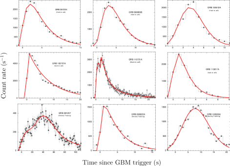
Figure 1: Background subtracted LCs of the GRBs in the energy range of NaI detector. We use the detector which has the highest count rate. Upper 6 panels: “hard-to-soft” (HTS) pulses, and lower 3 panels: “intensity tracking” (IT) pulses. LCs are fitted with exponential model (Norris et al. 2005). The values of the corresponding best-fit parameters are given in Table 2. Source: Basak & Rao (2014).

3 Results of Timing Analysis

We generate the light curve (LC) of each GRB in the 8-900 keV band of one NaI detector having maximum count rate (Figure 1). The LCs are fitted with Norris model. The best-fit values of the model parameters are shown in Table 2. We note that the pulse profiles of all the GRBs are adequately captured by Norris model (Figure 1). However, we note that $\chi^{2}_{red}$ of these fits are generally high. This is expected as the Norris model only captures the broad pulses, and does not account for the finer variability (see Rao et al. 2011). Our motivation to fit the LCs is to quantify the pulse width and asymmetry of the global pulse structure (see below). Hence, Norris model is adequate for this purpose.

In Table 2, we have also shown the derived parameters — the pulse peak position ($p$), width ($w$) and asymmetry ($\kappa$). These quantities are derived following Norris et al. (2005). The errors in the derived parameters are found by propagating the errors of the model parameters. However, error in $p$ is obtained by $\triangle\chi^{2}=2.7$ by directly tabulating $\chi^{2}$ for different values of $p$. This is because, the the correlation between $\tau_{1}$ and $\tau_{2}$ leads to large errors in $p$, particularly for the symmetric pulses. The derived errors in $w$ and $\kappa$, however, are small. From Figure 1, we see that though in general the GRBs have single broad pulse structures, in two cases we find evidence of multiple pulses. For GRB 081207, which is a very long GRB in comparison to the other GRBs, we find two pulses in the main bursting period. We also find two pulses for GRB 110721A ($\Delta\chi^{2}=205.1$ is found for an additional pulse). Hence, one has to be cautious while interpreting the results obtained for these two GRBs.

In Table 2 and Figure 1, the first 6 GRBs are categorized as HTS, and the rest as IT GRBs (section 4.3.2). By comparing the LCs and the values of asymmetry ($\kappa$) of these two classes, we find no trend in the asymmetry that can characterize any particular class. We find that two HTS GRBs (GRB 100707A, and the first pulse of GRB 110721A) have the highest asymmetry ($0.72\pm 0.01$, and $0.83\pm 0.05$, respectively). However, GRB 100612A (a HTS GRB) is very symmetric ($\kappa=0.14\pm 0.02$ only). Moreover, GRB 090922A, and the first pulse of GRB 081207 (IT GRBs) are very asymmetric ($0.62\pm 0.05$, and $0.57\pm 0.06$, respectively). Though we should be cautious about GRB 081207, it is clear that HTS and IT GRBs do not show any preference for asymmetry in their respective LCs.

4 Spectral Analysis

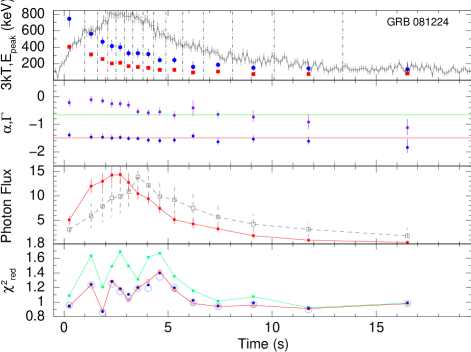
Figure 2: Analysis of GRB 081224. Panel 1: Evolution of $E_{\rm peak}$ (blue filled circles), and 3kT (red filled boxes) with time are shown. The corresponding LCs are shown in background. The LCs are plotted with the same scale as in Figure 1. The time intervals chosen for spectral analysis are shown by dot-dashed lines. We show the parameters at the mean time of each of the intervals. Panel 2: Evolution of $\Gamma$ (blue circles) of BBPL, and $\alpha$ (violet boxes) of Band function are shown. The “synchrotron lines of death” are shown at -3/2 and -2/3 values. Panel 3: Flux (photons cm^-2 s^-1) evolution of different components of BBPL model is shown. BB flux evolution is shown by the filled boxes (joined by continuous line), and PL flux, scaled with the total BB flux is shown by open boxes (joined by dashed line). Panel 4: $\chi^{\rm 2}_{\rm red}$ shown for Band (red open circles), BBPL (green filled boxes), mBBPL (blue filled circles), and 2BBPL (light blue open circles)

1 Choice Of Time-resolved Spectral Bins

We now turn to the time-resolved spectral analysis of the GRBs. For time-resolved study, the LC of a GRB is divided by requiring minimum counts $C_{\rm min}=1200$ i.e., $\sim 35\sigma$ (background subtracted) per time bin. We use one of the NaI detectors (section 4.3.1) having the highest count rate as the reference LC. The time divisions are achieved by integrating the LC from a start time ($T_{\rm s}$) till this required $C_{\rm min}$ is reached. Note that we do not require a definite $T_{\rm s}$ for integration. All we need is equal statistics in each bin. In all cases, we have chosen $T_{\rm s}\leq T_{0}$ (trigger time) to use as much data as possible. The choice of $C_{\rm min}$ depends on two competitive requirements: (i) The bins must be wide enough to give enough count, and (ii) small enough to capture the evolution. Note that the errors in the model parameters are dependent on the total flux in a bin. An approximate choice of total flux in a bin can be made such that the error in the evolving parameter (e.g., $E_{\rm peak}$) should be comparable to the variation. We have found that this is the case for a $\sim 0.5$ s bin size at the peak. As all the GRBs have $\sim 2500$ count rate at the peak (except GRB 100707A), we choose 1200 counts/bin, which is essentially the same as in Lu12. For GRB 100707A, which has $\sim 5000$ counts at the peak, we set $C_{\rm min}=2500$ count/bin (i.e., 50$\sigma$). We use $\chi^{2}$ minimization technique to estimate the model parameters. Note that the choice of $C_{\rm min}$ is also reasonable for $\chi^{2}$ method, as the estimated parameters have a maximum deviation of 10% from those determined by C-stat for a count of 1000 (Nousek & Shue 1989).

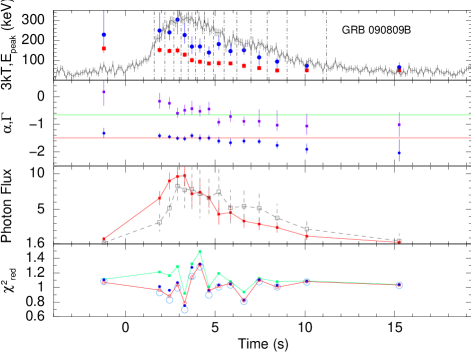
Figure 3: Analysis of GRB 090809B. The symbols used here are the same as Figure 2

For spectral analysis, we choose three NaI detectors, and one BGO detector. The detectors used for the individual cases are shown in Table 2. Note that due to the lower effective area, BGO detectors are mostly redundant for time-resolved study (e.g., Ghirlanda et al. 2010b). We found that the count rate in the BGO energy bins are often less than 2$\sigma$, particularly at energies above $\sim 500$ keV. However, to constrain the high energy portion of the spectral function, we use the BGO detector with heavy binning (5 to 7 logarithmic bins). The spectrum of the NaI, on the other hand, is binned by requiring 40 counts per bin. In Table 2, we have shown the start ($t_{1}$) and stop ($t_{2}$) time, and the number of bins ($n$) for the time-resolved spectral analysis. For GRB 081207, as we note another pulse at $>80$ s, we use the data till 76 s. However, this selection will not alter any conclusion we make for this GRB.

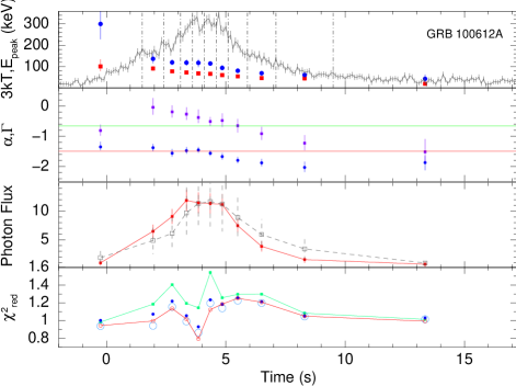
Figure 4: Analysis of GRB 100612A. The symbols used here are the same as Figure 2

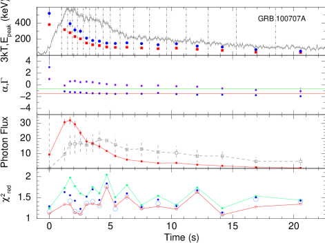
Figure 5: Analysis of GRB 100707A. The symbols used here are the same as Figure 2

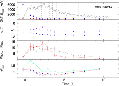
Figure 6: Analysis of GRB 110721A. The symbols used here are the same as Figure 2

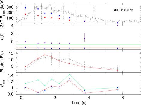
Figure 7: Analysis of GRB 110817A. The symbols used here are the same as Figure 2

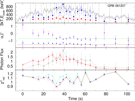
Figure 8: Analysis of GRB 081207. The symbols used here are the same as Figure 2

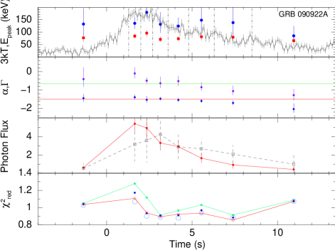
Figure 9: Analysis of GRB 090922A. The symbols used here are the same as Figure 2

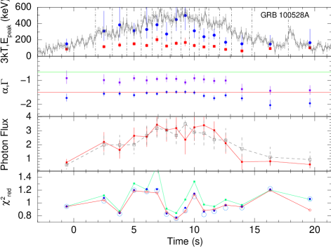
Figure 10: Analysis of GRB 100528A. The symbols used here are the same as Figure 2

2 Results Of Time-resolved Spectroscopy

A. Evolution Of $\bf E_{\rm\bf peak}$ And HTS-IT Classification

In Figure 2 through Figure 10, we have shown the results of our time-resolved spectral analysis of all the GRBs. The upper panels show the evolution of $E_{\rm peak}$ of the Band function, and $kT$ of the BBPL model as a function of time. The LCs of the individual GRBs are shown in grey colour to clearly show the evolution. The dot-dashed lines show the time divisions of the time-resolved spectral study. The values of the parameters are shown at the mean of $t_{1}$ and $t_{2}$. From the evolution of $E_{\rm peak}$, we see that the first 6 GRBs belong to HTS class, i.e., $E_{\rm peak}$ starts with a high value and decreases monotonically. The next 3 GRBs are IT GRBs, with $E_{\rm peak}$ tracking the pulse LC. Note that as the pulse LC is low-to-high-to-low, $E_{\rm peak}$ evolution can as well be said a soft-to-hard-to-soft (SHS) evolution (as discussed in chapter 3). Another important fact we find by comparing the $E_{\rm peak}$ and $kT$ evolution is as follows. In this panel, we have plotted the $3kT$ rather than kT to show the peak of the BBPL. Though the evolution of $E_{\rm peak}$ and $kT$ generally agrees, the $\nu F_{\nu}$ peak of the Band function is always higher than the corresponding peak of the BBPL model ($3kT$).

B. Evolution Of The Spectral Index

The evolution of the index are compared in the second panels from the top. We have shown the low energy index $\alpha$ of the Band function (violet boxes), and PL index ($\Gamma$) of the BBPL model (Please do not confuse $\Gamma$ of BBPL with bulk Lorentz factor). The two lines of death of synchrotron emission are shown by green line ($\alpha=-2/3$, i.e., slow cooling regime), and red line ($\alpha=-3/2$, i.e., fast cooling regime). We first note that the general trend of $\alpha$ evolution is high values to low values. Also, the value of $\alpha$ is always found greater than -3/2. In order to quantify the significance of the deviation from the predicted spectrum of fast cooling electrons, we find the following quantities. (i) We find the mean value of $\alpha$, and the deviation of the mean from $\alpha=-3/2$ in the units of $\sigma$. (ii) We assume $\alpha=-3/2$ as the model spectrum, and find the $\chi^{2}$ of the fit. The mean values of $\alpha$ are shown in Table 3 (4th column). The calculated errors in the means are 1$\sigma$, and these are calculated by using the two tailed nominal 90% errors of $\alpha$. Column 5 shows the first quantity, i.e., the deviation of mean $\alpha$ from $\alpha=-3/2$ in the units of $\sigma$. The significance of the trend as denoted by the $\chi^{2}_{\rm red}$ is shown in parenthesis. In each GRB, we see that the deviation is quite significant. In some GRBs, we see that the mean $\alpha$ is even greater than -2/3, the slow cooling line. However, the deviation from $\alpha=-2/3$ is not always significant. For some of the HTS GRBs, we found a significant deviation. For example, GRB 100707A (40$\sigma$), GRB 081224 (5.8$\sigma$), and GRB 110817A (5.0$\sigma$). For IT GRBs, we found no significant deviation from $\alpha=-2/3$ (all deviation are within 1$\sigma$). For IT GRB 100528A, we found a mean $\alpha=-1.02\pm 0.04$, which is well within the slow cooling line of death (at 8.8$\sigma$). In fact, we found that the values of $\alpha$ is always less than -2/3 for this GRB. We find another extreme case — GRB 110817A, which is a HTS GRB, the value of $\alpha$ is always greater than -2/3. From this discussion, we see that the HTS GRBs have a general preference of higher (harder) value of $\alpha$. Another important trend is shown by the PL index ($\Gamma$) of the BBPL model. This can be seen from the second panels of Figure 2 through Figure 10. It is apparent that $\Gamma$ has a preference for the value -3/2, which is exactly the index of synchrotron emission predicted for the fast cooling electrons. In Table 1, we have shown the deviation of mean value of $\Gamma$ from -3/2, and the $\chi^{2}_{\rm red}$ of the $\Gamma=-3/2$ fit. Note that the value of $\Gamma$ generally clusters near -3/2 almost in all cases (very low $\sigma$ deviation). The $\chi^{2}_{\rm red}$, which shows the significance of the deviations are small compared to the deviation of $\alpha$.

Table 1: Deviation of $\Gamma$ from -3/2 line

GRB	$\chi^{2}_{\rm red}$ (dof) for $\Gamma=-\frac{3}{2}$ fit	Mean $\Gamma$	Deviation from $\Gamma=-\frac{3}{2}$ (in $\sigma$)
081224	0.49 (15)	$-1.52\pm 0.03$	$0.67\sigma(\downarrow)^{(a)}$
090809B	1.03 (15)	$-1.53\pm 0.03$	$1.0\sigma(\downarrow)$
100612A	2.86 (11)	$-1.60\pm 0.04$	$2.5\sigma(\downarrow)$
100707A	4.58 (18)	$-1.41\pm 0.02$	$4.5\sigma(\uparrow)$
110721A	6.86 (15)	$-1.50\pm 0.01$	$<0.4\sigma(\uparrow)$
110817A	0.54 (8)	$-1.57\pm 0.04$	$1.75\sigma(\downarrow)$
081207	1.86 (20)	$-1.36\pm 0.03$	$3.5\sigma(\uparrow)$
090922A	0.87 (8)	$-1.55\pm 0.05$	$1.0\sigma(\downarrow)$
090922A	1.63 (16)	$-1.57\pm 0.02$	$3.5\sigma(\downarrow)$

^(a) $\uparrow$ (or $\downarrow$) denotes the value of $\Gamma>$ (or $<$) -3/2

C. Flux Evolution

In the third panels of the figures, we have plotted the flux evolution of the BB and PL component. Interestingly, for three GRBs, namely GRB 081224, GRB 100707A and GRB 110721A, we see a distinct behaviour of the PL flux from the BB flux. The PL flux is evidently delayed from the BB. Also, the PL tends to linger at the late phase of the prompt emission. In chapter 6, we shall discuss the delay of the PL component of 2BBPL model, and show that the delayed and lingering behaviour of the PL component has a remarkable similarity with the high energy (GeV) evolution. As for the current study, we find reported Fermi/LAT detection (LLE data) for these three GRBs in our sample, i.e., these GRBs accompany high energy (GeV) emission (see chapter 6 for extensive discussion). Ackermann et al. (2013) report the following LAT detection levels — 3.1$\sigma$ (GRB 081224), 3.7$\sigma$ (GRB 100707A), and 30.0$\sigma$ (GRB 110721A)

D. A Comparative Study

Finally, the $\chi^{2}_{\rm red}$ of all the models are shown in panel 4. As we have seen interesting results by applying BBPL model for the spectral fitting, it is interesting to compare this model with Band function. However, we note that $\chi^{2}_{\rm red}$ of the BBPL model (green boxes) are generally worse than those of the Band function (blue filled circles). To quantify the superiority of the Band function over BBPL, we perform $F$-test assuming BBPL as the original (null) hypothesis, and Band function as the alternative hypothesis. Note that as these models are not nested, the F-test is different from the general F-test procedure used for nested models. For each time-resolved bin of a GRB, we calculate the confidence level (CL) of rejecting the original hypothesis as compared to the alternative model (Band). We compute the mean ($\langle\rm CL\rangle$), and standard deviation (SD) of the CLs (see Table 3). It is clear from the comparison of HTS and IT classes that BBPL model better fits the spectrum of IT GRBs (also see Figure 8,  9, and  10). But for HTS class, in general, Band shows much better $\chi^{2}_{\rm red}$. Hence, BBPL model may be more physical than the Band function, but the BB component is probably an approximation of a more physical function. The obvious choice are multi-colour BB (mBB), or two BBs (2BB). Note that both these models have comparable $\chi^{2}_{\rm red}$ (in the range 0.8-1.2) as the Band function. Hence, one of these models is preferred for spectral study. Note that both of these models are extension of the simple BBPL model, hence, all the interesting results of BBPL model, e.g., -3/2 PL index, delayed PL evolution etc., should hold for both of them (see chapter 6).

The results of our detailed analysis are summarized in Table 3. Based on the above discussions, we can draw some approximate, but important conclusions regarding HTS and IT classes. We note the following differences.

• (i) The HTS GRBs have generally higher values of $\alpha$ than the IT GRBs. Note that the significance of deviation of $\alpha$ from the -3/2 line is quite high for HTS GRBs. In 3 cases, we find significant deviation even from -2/3 line. In 63.4% cases of HTS pulses, $\alpha$ is greater than -2/3. The only exception of this trend is GRB 110721A. Exclusion of this GRB leads to 74.6% such cases. The IT GRBs, on the other hand, shows generally lower values of $\alpha$. Though the $\alpha$ of IT GRBs also show high deviation from -3/2 line, the $\chi^{2}_{\rm red}$ are generally lower than those of HTS GRBs (see Table 3). In only 44% cases, the value of $\alpha$ is found to be greater than -2/3. Also, as discussed, the mean value of $\alpha$ has an insignificant deviation (within 1$\sigma$) from -2/3 in all IT GRBs. Finally, the HTS GRB 110817A has $\alpha$ always greater than -2/3, with mean deviation of $5\sigma$, while the IT GRB 100528A has $\alpha$ always less than -2/3, with mean deviation of $8.8\sigma$.

• (ii) We also study the trend of $\alpha$ evolution with time. In Figure 11 (left panel), the values of $\alpha$ are plotted in the x-axis, with time sequence in the y-axis. We have also indicated the -3/2 and -2/3 death lines by red and purple solid lines. We note that the value of $\alpha$ generally becomes lower (softer) at the later part (right to left transition). This possibly indicates that the synchrotron emission, if present, dominates at the later phase. We have marked the HTS (red circles) and IT (black open boxes) GRBs to show the evolution of each class. We note that the evolution of $\alpha$ is generally high-to-low values. In the right panel of the figure, we have plotted the $\alpha$ values in ascending order to visualize the deviations from the death lines. It is clear from this panel that the $\alpha<-2/3$ region (left of the purple line) is mainly populated by IT GRBs, while majority of HTS GRBs have $\alpha>-2/3$ (right of the purple line).

• (iii) For HTS GRBs, the mean value of CL that Band function is preferred over BBPL fitting is 79.3%. For IT GRBs, the mean value is 67%.

• (iv) Note that the LAT detection is found only for 3 HTS GRBs, and none of the IT GRBs.

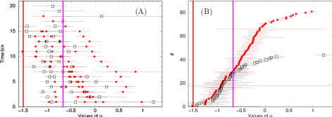
Figure 11: Low energy index ($\alpha$) for the GRBs in our sample — HTS (filled circles), and IT (open boxes). The errors are measured at nominal 90% confidence level. (A) For each GRB, the distribution of $\alpha$ (x-axis) of each time-resolved bin is plotted with the time sequence (y-axis). The values of $\alpha$ show higher deviation from the synchrotron death lines ($\alpha=-3/2$: red line, $\alpha=-2/3$: purple line) at the earlier times. (B) $\alpha$ values, sorted in ascending order to show the deviations. Its value is always greater than -3/2 (for significance, see Table 3). The region where $\alpha<-2/3$ (i.e., within the slow cooling regime of synchrotron emission) is significantly populated by IT GRBs (see the left side of the purple line), while $\alpha>-2/3$ region is generally acquired by HTS pulses. The mean value of $\alpha$ for HTS and IT GRBs are -0.42 and -0.68, respectively

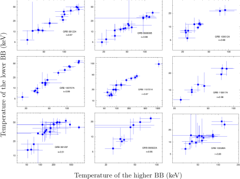
Figure 12: The correlation between the temperature (kT) of the two BBs of 2BBPL model are shown. A significant correlation is found in each case. Upper 6 panels: HTS GRBs. Lower 3 panels: IT GRBs

5 Summary And Discussion

To summarize, we have investigated the timing and spectral properties of GRBs with single pulses. We have applied four models, namely Band, BBPL, mBBPL and 2BBPL for time-resolved spectroscopy of the pulses. We found that the value of $\alpha$ of the Band function is significantly higher than the fast cooling line $\alpha=-3/2$, and in many cases, even higher than $\alpha=-2/3$ line with reasonable significance. Hence, a synchrotron interpretation is unacceptable. At least the spectrum should have other contributors e.g., the emission from the photosphere. In this spirit, we have applied the BBPL model (following earlier works), and have found interesting results e.g., the PL index of the BBPL model ($\Gamma$) has a preference for -3/2 value, showing a remarkable consistency with the synchrotron origin of the PL component. However, we have found that the $\chi^{2}_{red}$ of BBPL model is generally worse than that of the Band function. The other two functions, namely mBBPL and 2BBPL models have comparable $\chi^{2}_{red}$ as the Band function. Hence, mBBPL and 2BBPL are the preferred models for our set of GRBs. As these models are modification of the thermal component of the BBPL model, we expect the PL component to show similar behaviour (see the next chapters).

Based on the peak energy evolution, we have found that the pulses can belong to either HTS or IT (or, SHS) class. As we have chosen only single pulse GRBs, the IT evolution cannot have any overlapping effect. By performing a detailed spectral analysis, we have found interesting differences of these two classes, though the origin is not clear at the moment. We have also found delayed and lingering behaviour of the PL component for 3 GRBs, and interestingly, these GRBs are accompanied by high energy (GeV) emission.

Finally, we have used a new model, namely 2BBPL which gives comparable fit as mBBPL model. Though the physical mechanism of this model is not known at this moment, in the next chapter, we shall try to give some important evidences in support of this model. We shall also show the predictive power of this model in chapter 6. Before finishing this chapter, let us show one of the most important feature of 2BBPL model, which we shall use in subsequent analyses. In Figure 12, we have shown the temperature (kT) of the two BBs of 2BBPL model. It is evident from the figure that the two BB temperatures are highly correlated. The correlation coefficient ($r$) are generally high (0.51-0.99). There can be two reasons for such correlation, first, the 2BBPL may be an approximation of a more fundamental function. In this case, the correlation is a natural consequence of the approximation. Second, the 2BBPL is indeed a physical model. It may be an approximate function, but all the components have distinct source of emission. However, the sources of the 2BBs must have some common feature which leads to the observed correlation. In the subsequent chapters, we shall try to give evidences in favour a physical origin of the 2BBPL model.

Table 2: Parameters of Norris model fit to the LCs of the GRBs. We also show the time interval ($t_{1}$ to $t_{2}$), total number of time-resolved bins ($n$), and the detectors which are used for the time-resolved spectroscopy.

GRB	Norris Model parameters							Specification of time-resolved analysis
	$t_{s}$ (s)	$\tau_{1}$ (s)	$\tau_{2}$ (s)	$\chi^{2}_{red}(dof)$	p (s)	w (s)	$\kappa$	$t_{1}$,$t_{2}$ (s)	$n$	Detectors used
081224	$-1.53_{-0.26}^{+0.34}$	$3.60_{-1.07}^{+0.99}$	$3.30_{-0.21}^{+0.27}$	6.80 (13)	$1.90\pm 0.10$	$7.5\pm 0.7$	$0.44\pm 0.03$	-0.5, 19.6	15	n6, n7, n9, b1
090809B	$-1.74_{-0.38}^{+0.31}$	$9.35_{-1.85}^{+2.59}$	$2.50_{-0.17}^{+0.17}$	5.88 (13)	$3.10\pm 0.09$	$7.4\pm 0.6$	$0.34\pm 0.02$	-4.0, 19.3	15	n3, n4, n5, b0
100612A	$-8.43_{-2.65}^{+1.61}$	$156.4_{-57.4}^{+137.6}$	$0.88_{-0.17}^{+0.14}$	16.8 (9)	$3.30\pm 0.06$	$6.5\pm 1.5$	$0.14\pm 0.02$	-2.0, 17.2	11	n3, n4, n8, b0
100707A	$-2.5_{-2.6}^{+3.2}\times 10^{-2}$	$0.37_{-0.05}^{+0.04}$	$7.19_{-0.16}^{+0.18}$	4.01 (233)	$1.60\pm 0.07$	$9.9\pm 0.28$	$0.72\pm 0.01$	-1.0, 22.6	18	n4, n7, n8, b1
110721A	$-0.62_{-0.15}^{+0.08}$	$1.58_{-0.46}^{+0.67}$	$1.59_{-0.23}^{+0.15}$	1.32 (229)	$0.96\pm 0.10$	$3.55\pm 0.62$	$0.45\pm 0.03$	-1.0, 10.6	15	n6, n7, n9, b1
	$1.75_{-0.07}^{+0.10}$	$0.079_{-0.053}^{+0.074}$	$6.75_{-0.66}^{+0.86}$		$2.48\pm 0.12$	$8.08\pm 1.04$	$0.83\pm 0.05$
110817A	$-0.62_{-0.42}^{+0.30}$	$1.11_{-0.66}^{+1.31}$	$1.76_{-0.24}^{+0.24}$	1.85 (8)	$0.78\pm 0.12$	$3.6\pm 0.8$	$0.49\pm 0.08$	-0.3, 7.1	8	n6, n7, n9, b1
081207	$-8.55_{-2.21}^{+3.30}$	$14.14_{-6.10}^{+9.10}$	$50.79_{-10.22}^{+11.10}$	1.36 (114)	$18.25\pm 3.36$	$90\pm 21$	$0.57\pm 0.06$	-7.0, 76.0	20	n1, n9, na, b1
	$-9.64$	$304.7$	$9.24_{-2.20}^{+3.50}$		$43.42\pm 1.19$	$45$	$0.20$
090922A	$-0.39_{-0.19}^{+0.15}$	$0.62_{-0.27}^{+0.38}$	$4.00_{-0.30}^{+0.30}$	6.23 (15)	$1.18\pm 0.18$	$6.4\pm 0.7$	$0.62\pm 0.05$	-4.0, 13.4	8	n0, n6, n9, b1
100528A	$-32.6_{-2.36}^{+2.36}$	$1262.0_{-61.1}^{+60.9}$	$1.29_{-0.38}^{+0.14}$	6.56 (21)	$7.70\pm 0.06$	$14.5\pm 3.0$	$0.09\pm 0.004$	-3.0, 21.4	16	n6, n7, n9, b1

Table 3: Classification of the GRBs based on the spectral analysis: “hard-to-soft” (HTS), and “intensity tracking” (IT)

GRB	Type	Behaviour of	Mean $\alpha$	Deviation of $\alpha$ (a)	$\alpha$ crossing -2/3	Band/BBPL(b)	LAT detection
		the PL Flux		from -3/2 ($\chi^{2}_{\rm red}$)	“line of death”
081224	HTS	Clear delay and lingering	$-0.43\pm 0.04$	26.7$\sigma$ (53.5)	11/15	0.80 (0.14)	3.1$\sigma$
090809B	HTS	Mild delay and lingering	$-0.64\pm 0.06$	14.3$\sigma$ (13.5)	8/15	0.74 (0.15)	No
100612A	HTS	Very mild lingering	$-0.58\pm 0.07$	13.1$\sigma$ (19.1)	7/11	0.73 (0.15)	No
100707A	HTS	Clear delay and lingering	$0.013\pm 0.017$	89.0$\sigma$ (71.6)	16/18	0.74 (0.23)	3.7$\sigma$
110721A	HTS	Clear delay and lingering	$-0.95\pm 0.02$	27.5$\sigma$ (56.2)	2/15	0.94 (0.10)	30.0$\sigma$
110817A	HTS	Mild lingering	$-0.31\pm 0.07$	16.9$\sigma$ (34.1)	8/8	0.81 (0.09)	No
081207	IT	Mild delay	$-0.63\pm 0.06$	14.5$\sigma$ (10.5)	10/20	0.66 (0.12)	No
090922A	IT	Mild delay and lingering	$-0.66\pm 0.10$	8.4$\sigma$ (9.7)	5/8	0.67 (0.13)	No
100528A	IT	Mild lingering	$-1.02\pm 0.04$	12.0$\sigma$ (9.8)	0/16	0.68 (0.14)	No

^(a) Here deviation is quantified as the difference of the mean value of $\alpha$ ($\langle\alpha\rangle$) from the fast cooling “line of death” (i.e., $\alpha=-3/2$ line) in the units of $\sigma$. The $\chi^{2}_{red}$ is calculated by fitting $\alpha$ values assuming the model $\alpha=-3/2$. Hence, higher the value, higher is the deviation from the fast cooling synchrotron emission.
^(b) Band function is compared to the BBPL model. We have performed F-test for all time-resolved spectrum to find the confidence level (CL) of alternative model (i.e., Band function) over the original model (i.e., BBPL model). The quantity shown here is the mean (and standard deviation) of CL of the F-test for each GRB.

Chapter 5 Parametrized Joint Fit

1 Overview

In the previous chapter, we have discussed the alternative models of the prompt emission spectrum of GRBs. We specifically chose GRBs with single pulses and high flux for our study. The primary motivation of selecting single pulses was to get an idea about the parameter variations within a pulse which is essentially unaffected by the overlapping effect. We also wanted to know whether the $E_{\rm peak}$ evolution is always hard-to-soft (HTS), or there are intensity-tracking (IT) behaviours as well. We have found that the $E_{\rm peak}$ evolution within some of the pulses are indeed HTS. However, we have also found pulses which rather show the IT evolution. The finding of such a spectral evolution in a single pulse undoubtedly tells us that the IT evolution is real, and cannot be always a superposition effect of two HTS pulses. Though the physical reason for these two distinct behaviours are not known at present, but we can use these evolution properties to get a better handle on the time-resolved spectral study, which is the subject of this chapter. Aided with the knowledge of single pulses, we now turn our attention to GRBs with multiple (but separable) pulses (Basak & Rao 2013b). We shall also study some GRBs having high flux, but with more rapid variability (Rao et al. 2014).

1 Time-resolved Study With Parametrization

Time-resolved spectroscopy is a natural choice to study the time evolution of a spectrum. It is possible that a time-integrated spectrum appears completely different from the actual snap-shots of the spectrum. For example, Ryde (2004) have shown that an instantaneous spectrum is consistent with a blackbody and a power-law (BBPL) model, whereas the integrated spectrum appears as a Band function, and a BBPL model does not fit a time-integrated spectrum at all. Hence, one has to investigate the spectral evolution within as small time bin as possible. But, as discussed in the previous chapter, the choice of bin size is limited by the statistics, meaning, with a low flux data, one can fit any model. For example, Ghirlanda et al. (2010b) have studied the time-resolved data of 9 GRBs detected by the Fermi/GBM. Due to the requirement of fine bin size, they could use only a cut-off power-law (CPL), which is a three-parameter model. The parameters of a more complex function like Band cannot be constrained with such data quality. On the other hand, we cannot possibly afford to make a large bin size if we want to follow the time evolution.

The solution to our dilemma lies in the realization that the spectral evolution need not be too drastic. In fact, one can suitably parametrize the evolution in order to reduce the number of free parameters ($P_{f}$) of the description. For example, if we have $n$ time-resolved bins, a 4-parameter function, such as Band, requires $4n$ parameters in total to describe the time evolution. If we believe e.g., that $E_{\rm peak}$ evolution is HTS, and assume certain functional form of the time evolution, then effectively it reduces $P_{f}$ to $3n+1$. For a GRB with 20 s duration and 1 s uniform bin, we have $n=20$. Hence, such a scheme reduces the total number of parameters from 80 to 61. Note that such a strategy was indeed applied when we developed the simultaneous timing and spectral model of GRB pulses (chapter 3). Of course, we know that GRB pulses can also have IT evolution, and hence, we shall not assume a HTS evolution. In section 5.3, we shall describe our assumptions in detail. We shall specifically develop a new technique, named “parametrized joint fit” for the spectral analysis. The primary motivation of the method is quite apparent — we are aiming to reduce the number of model parameters in order to study the spectral evolution, and compare various models.

2 The Spectral Models

The models we use for the spectral study (as in the previous chapter) are: (i) Band, (ii) BBPL, (iii) mBBPL, and (iv) 2BBPL. Except for the Band function, which has a non-thermal spectral shape, all other models have a thermal and a non-thermal component. We have often seen that the Band function is unacceptable based on the fact that the low energy index ($\alpha$) has higher value than -3/2, and sometime the value even exceeds the slow cooling limit at -2/3. However, the goodness of a fit (in terms of $\chi^{2}_{\rm red}$) using a Band function is comparable to those of mBBPL and 2BBPL models. From a purely phenomenological point of view, a general spectrum has two regions of interest — the peak of the $\nu F_{\nu}$ spectrum, and the “wings” (i.e., the low and high energy parts). While a Band function has two slopes joining at the peak, each of the alternative functions have a thermal peak, and a single slope describing both the low and high energy parts. This slope is lower than the low energy slope ($\alpha$), and higher than the high energy slope ($\beta$) of the Band function. Hence, the PL component of these alternative models “hold” the spectrum at the wings. If the difference occurs in the peak then we immediately see the effect in the value of $\chi^{2}$. For example, BBPL model has a narrower peak than all other models. If the spectrum is not as narrow as a BB spectrum at the peak, the BBPL model should give an inferior fit. However, the peak of both mBBPL and 2BBPL are as broad as that of a Band function; the only difference occurs in the wing. As the statistics is low at the two ends of the detector’s energy band, we do not expect an order of magnitude improvement if the differences occur at the wings. This was precisely the reason that all these very different functions, namely, Band, mBBPL, and 2BBPL, gave similar values of $\chi^{2}$ while fitting the time-resolved data (see chapter 4). Hence, it is interesting to investigate how the models fit the data when we demand certain extra conditions on their individual parameter evolution. For example, we have seen that the two temperatures of the 2BBPL model are highly correlated. Hence, we shall assume a fixed factor for the two temperatures, and tie the temperature ratio in all time bins. If the temperatures are indeed correlated, we should still get good $\chi^{2}$ values. As a benefit, we shall reduce the number of free parameters ($P_{f}$), because determining the factor is enough to infer the temperature of one of the BBs, given the temperature of the other one.

Figure 1: The LC of GRB 081221 (background subtracted), fitted with Norris model (Norris et al. 2005). The LC is generated by adding the counts of two NaI ($n1$ and $n2$) and one BGO ($b0$) detector. Source: Basak & Rao (2013b).

2 Sample Selection

The requirements of our study are GRBs with high background subtracted counts and long enough duration for time-resolved study. In addition, we want GRBs with separable pulses. We use Nava et al. (2011) catalogue for selecting bright (fluence $\geq 10^{-6}$ erg), and long ($\delta t\geq 15$ s) GRBs with single/separable pulse (s). We find 11 such GRBs (see chapter 2, section 2.4.6). As GRB 081221 is the brightest GRB (fluence $=3.7\times 10^{-5}$ erg) in the sample, we use it for the time-resolved spectral study using our new technique. In Figure 1, we have shown the LC of the GRB, with the two pulses fitted by Norris model (Norris et al. 2005). In addition to this GRB, we shall use GRB 090618, which has high fluence ($=3.4\times 10^{-4}$ erg), and broad pulse structure. Apart from studying GRBs with clean pulses, it is also important to study GRBs with variable LC. In this regard, we shall discuss 3 GRBs, namely, GRB 080916C, GRB 090902B, and GRB 090926A. As these GRBs have highly variable time profile, some modification of our technique is required for them.

3 Assumptions Of The New Technique

We have the following parameters of various models for the spectral fitting.

• (i) Band function: normalization ($A_{b}$), photon indices ($\alpha$, and $\beta$), and peak energy ($E_{\rm peak}$)

• (ii) BBPL: temperature ($kT$) and normalization ($K_{1}$) of BB, and index ($\Gamma$) and normalization ($K_{2}$) of PL.

• (iii) mBBPL: the local disc temperature $kT(r)\propto r^{-p}$, where r is the distance from the centre of the disc. Hence, the parameters are inner temperature ($T_{in}$), index $p$, normalization of mBB ($K_{mbb}$), and PL index and normalization

• (iv) 2BBPL: two BB temperatures ($kT_{h}$, $kT_{l}$), normalizations ($N_{h}$, $N_{l}$), and PL index and normalization.

First, we divide the LC of a GRB into the constituent pulses e.g., GRB 081221 is divided into two pulses: -1.0 to 12.05 s, and 17.0 to 40.55 s. Note that the overlapping region is neglected to facilitate parametrization. We further divide each pulse into a rising and a falling sector. This is based on the fact that $kT$ evolution of BBPL model generally has a break near the peak flux. Ryde & Pe’er (2009) have studied a set of bright GBM GRBs, and have found that the time evolution of both flux and $kT$ have similar break time (within errors). Following the procedure of the previous chapter, we choose the start time of each sector and integrate the LC till we get a minimum count per bin $C_{\rm min}$.

1 Assumptions For The Band Function

For the Band function, we assume that the photon indices have little variation within a sector. Hence, the value of these parameters can be determined by tying the parameters in all time bins of a sector. Note that this tying will not only help us reducing $P_{f}$, but we can also study the differences in the spectral slopes in the rising and falling sectors. For example, we have seen that the value of $\alpha$ tend to be high at the beginning, and evolves to a lower value. Hence, by tying this parameter in each sector, we can find the contrast of the spectral slope, and can possibly comment more on the origin of the spectrum.

We further assume that $E_{\rm peak}$ evolution is a power-law function of time ($E_{\rm peak}\propto t^{\mu}$). As the evolution can be either HTS or IT type, we shall obtain the parameter $\mu$ independently in each sector. Note that ideally one should also put a start time for the parametrization. In our case, we have used this time either as zero, or -10 (for negative start time). As the parametrization is not corrected for the start time, the $\mu$ values in different pulses should not be compared. Finally, the normalization of Band function ($A_{b}$) is assumed as a free parameter of our model. With these assumptions we reduce $P_{f}$ from $4n$ to $n+4$, where $n$ is the number of time bins in a sector. The free parameters are $n$ normalizations, $\alpha$, $\beta$, $\mu$ and the peak energy at the starting time bin ($E_{\rm peak}(t_{0})$). The peak energy at any time can be found by $E_{\rm peak}(t_{0})\times(t/t_{0})^{\mu}$. Note that the choice of a time bin to specify the value of $E_{\rm peak}$ is arbitrary. All we require is the $E_{\rm peak}$ at any time bin, and $\mu$ to specify the evolution.

2 Assumptions For The BBPL Model

Following the scheme used for the Band function, we assume that the $kT$ of BBPL model has a power-law time evolution ($kT\propto t^{\mu}$) in each sector. We tie the index of PL spectral component in all bins of a sector. The parametrization of the normalization is more complicated than that of the Band function, as we have two normalizations ($K_{1}$ and $K_{2}$). We can either assume an overall free normalization, and parametrize $K_{1}$ and $K_{2}$, or we can parametrize one of the normalizations and treat the other as a free parameter. Note that in both of the cases, we get an equal number of parameters as the Band function. Ryde & Pe’er (2009) have investigated the parameter ${\cal{R}}=(F_{\rm BB}/\sigma T^{4})^{1/2}$, which either remain constant or increases with time, where $F_{\rm BB}$ is the observed BB flux. Now, if we assume that $F_{\rm BB}$ evolves as a simple function of time as $F_{\rm BB}\propto t^{\zeta}$, then ${\cal{R}}\propto t^{\zeta/2-2\mu}$. For $\mu\leq\zeta/4$, we expect the observed time evolution of ${\cal{R}}$. Hence, the BB normalization ($K_{1}$) can be chosen as a power-law function of time ($K_{1}\propto t^{\nu_{1}}$). Now, we can assume this parametrization and use the PL normalization ($K_{2}$) as a free parameter, and this will give us the same number of free parameters as the Band function. However, note that this scheme will put more constraints on the BBPL parametrization, as the overall norm is not a free parameter as the Band function. Hence, to overcome this situation, we also assume that the PL component has as smooth a time evolution as the BB component i.e., $K_{2}\propto t^{\nu_{2}}$. Now, we can make the overall normalization ($K$) as a free parameter by assuming the time evolution of the ratio of the normalization of BB and PL component as $K_{1}/K_{2}\propto t^{\nu_{1}/\nu_{2}}\propto t^{\nu}$. Thus the parametrized joint fit of the BBPL model has equal number of parameters as that of the Band function ($n+4$).

3 Assumptions For mBBPL And 2BBPL Models

For mBBPL we choose similar parametrization as the BBPL model. In addition, we tie the parameter $p$ in all the time bins of a sector. For 2BBPL model, we assume that the two temperatures ($kT_{h}$, $kT_{l}$), and the normalizations ($N_{h}$, $N_{l}$) are highly correlated. Hence, we tie their ratio in each sector. Compared to Band and BBPL, these models have one more, and two more parameters, respectively. For example, if we have 25 time-resolved bins, then a Band model without parametrization would require $25\times 4=100$ free parameters. Using the technique as described above, this number is respectively reduced to 29 (for Band and BBPL), 30 (for mBBPL) and 31 (for 2BBPL). In Figure 2, we have shown $P_{f}$ as a function of the number of time bins. As the number of bins increases, we gain in terms of $P_{f}$. The models using the new technique give similar $P_{f}$.

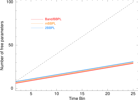
Figure 2: Number of free parameters ($P_{f}$) as a function of number of time bins ($n$) is shown. The dashed line shows the number of parameters ($4n$) required for a normal time-resolved spectroscopy using Band/BBPL model. The solid lines show that required by the parametrized joint fit technique for all the models. $P_{f}$ is comparable for all the models using the new technique.

4 Time-resolved Spectral Analysis of GRB 081221

We shall start with a time-resolved spectral study of GRB 081221 (see Figure 1) to validate the assumptions of the parametrized joint fit technique. In order to check whether the choice of bin size makes any effect on the analysis, we try various schemes to extract the time-resolved data (i) We choose 3 s uniform time bin to extract the time-resolved data. (ii) Later, we shall also use a finer bin size of 1 s uniform bin to check whether finer bin changes any conclusion we make. (iii) Finally we shall choose unequal bins by requiring minimum count per bin ($C_{\rm min}$) for the parametrized joint fit technique.

Figure 3: Comparison between $\chi^{2}_{\rm red}$ obtained by fitting Band, BBPL ($\Gamma$ thawed and frozen cases), mBBPL, and 2BBPL models to the time-resolved spectra of GRB 081221. The markers are explained in the inset. We draw lines to join $\chi^{2}_{\rm red}$ points obtained by BBPL ($\Gamma$ free case) fitting (solid line), and those obtained by 2BBPL fitting (dot-dashed line) to the spectral data. Source Basak & Rao (2013b).

1 Case I: Uniform Bin of 3.0 s

First, we choose 3.0 s uniform bin size, and obtain a total of 14 time-resolved bins starting with -1.0 s. Among these time bins the first pulse contains approximately the first four bins, while the second pulse contains the last 8 bins. The two intermediate bins belong to the overlapping region of the two pulses. In Table 1, we have shown the time bins by numbering them 0-13. We fit the time-resolved data with Band and BBPL model. The corresponding model parameters and $\chi^{2}_{\rm red}$ are reported in the table. As we want to tie the PL index ($\Gamma$) in each sector (rising and falling part) of a pulse for the parametrized joint fit, let us investigate the effect of freezing this parameter in each pulse. From the table, we first note that the value of $\Gamma$ remains almost constant in the major portion of each pulse (note that we have shown -$\Gamma$ for convenience). We calculate the average value of $\Gamma$ in each pulse and find $\Gamma=-1.83$ in each case, with a dispersion of 0.14 and 0.10 in the respective pulses. The average value of $\Gamma$ is determined by using the values of 0-2 bins and 6-11 bins of the first and second pulse, respectively. We have neglected the overlapping regions and the low flux bins for calculating the average. We now freeze the value of $\Gamma$ at -1.83 and perform the spectral analysis again. The corresponding values are also shown in the table. By comparing the values of the parameters, we note that the assumption of constant $\Gamma$ does not change the spectral parameters significantly.

In Figure 3, we plot $\chi_{red}^{2}$ obtained by fitting a BBPL with free $\Gamma$ (filled circles), BBPL with frozen $\Gamma$ (open circles), and Band function (stars). We note that the two cases of BBPL fitting have remarkably similar $\chi_{red}^{2}$. Hence, freezing $\Gamma$ essentially does not affect the statistics. In fact, it points towards the fact that the data is consistent with a BBPL model with the PL index constant throughout a pulse. We also note that the BBPL model is inferior to the Band function specially in the second pulse. We now fit the time-resolved spectra with mBBPL and 2BBPL models. A comparison of the mBBPL (filled boxes) and 2BBPL (pluses) models with the Band function clearly shows that all these models have similar $\chi_{red}^{2}$ throughout (Figure 3).

Table 1: Results of fitting the time-resolved spectra of GRB 081221 with Band and BBPL function. For BBPL fitting, we study two cases, namely, PL index ($\Gamma$) free, and frozen to the mean value -1.83 which is obtained during the highest count rate region.

Bin(a)	BBPL ($\Gamma$ free)					BBPL ($\Gamma$ frozen to 1.83)				Band
#	$kT$	$K_{1}^{(b)}$	$-\Gamma^{(c)}$	$K_{2}$	$\chi^{2}_{red}(dof)$	$kT$	$K_{1}$	$K_{2}$	$\chi^{2}_{red}(dof)$	$\alpha$	$\beta$	$E_{peak}$	$\chi^{2}_{red}(dof)$
0	$38.03_{-4.28}^{+4.91}$	$2.99_{-0.68}^{+0.67}$	$1.73_{-0.25}^{+0.42}$	$5.31_{-3.15}^{+12.72}$	$1.03(67)$	$38.28_{-3.97}^{+4.78}$	$3.14_{-0.46}^{+0.49}$	$7.18_{-2.16}^{+2.25}$	$1.01(68)$	$-0.28_{-0.30}^{+0.36}$	$-10.0$	$178.06_{-27.57}^{+42.39}$	$1.03(67)$
1	$16.26_{-2.21}^{+2.45}$	$1.76_{-0.36}^{+0.39}$	$1.77_{-0.13}^{+0.15}$	$14.27_{-5.98}^{+9.51}$	$1.34(76)$	$16.92_{-1.63}^{+1.87}$	$1.83_{-0.33}^{+0.34}$	$17.33_{-2.99}^{+3.08}$	$1.33(77)$	$-0.69_{-0.22}^{+0.39}$	$-3.76_{-\infty}^{+1.30}$	$77.92_{-15.58}^{+11.08}$	$1.10(76)$
2	$10.14_{-2.07}^{+3.12}$	$0.78_{-0.27}^{+0.28}$	$1.99_{-0.23}^{+0.27}$	$20.66_{-13.36}^{+28.87}$	$1.02(67)$	$9.07_{-1.33}^{+1.49}$	$0.84_{-0.25}^{+0.26}$	$10.94_{-3.10}^{+3.28}$	$1.02(68)$	$-0.24_{-1.10}^{+1.64}$	$-2.55_{-\infty}^{+0.29}$	$35.41_{-8.53}^{+18.41}$	$0.98(67)$
3	$10.98_{-2.14}^{+2.56}$	$0.74_{-0.27}^{+0.31}$	$2.16_{-0.25}^{+0.40}$	$32.99_{-20.23}^{+65.24}$	$0.94(69)$	$9.07_{-1.32}^{+1.39}$	$0.80_{-0.24}^{+0.26}$	$9.21_{-2.87}^{+3.02}$	$0.99(70)$	$-0.85_{-0.54}^{+0.80}$	$-3.07_{-\infty}^{+0.62}$	$39.74_{-7.77}^{+8.60}$	$0.93(69)$
4	$6.82_{-1.13}^{+1.69}$	$0.61_{-0.26}^{+0.28}$	$1.85_{-0.34}^{+0.27}$	$9.05_{-7.42}^{+17.99}$	$0.92(134)$	$6.76_{-1.08}^{+1.17}$	$0.63_{-0.20}^{+0.21}$	$8.13_{-2.71}^{+2.89}$	$0.91(135)$	$0.52_{-1.60}^{+3.16}$	$-2.47_{-0.54}^{+0.25}$	$24.48_{-5.39}^{+9.05}$	$0.92(134)$
5	$11.36_{-1.74}^{+2.01}$	$1.12_{-0.29}^{+0.30}$	$2.08_{-0.13}^{+0.16}$	$49.09_{-19.27}^{+31.10}$	$0.91(147)$	$9.18_{-1.02}^{+1.06}$	$1.19_{-0.26}^{+0.27}$	$18.14_{-3.07}^{+3.19}$	$0.97(148)$	$-1.06_{-0.32}^{+0.46}$	$-2.92_{-\infty}^{+0.45}$	$43.19_{-7.51}^{+7.34}$	$0.88(147)$
6	$22.61_{-0.99}^{+1.00}$	$8.52_{-0.65}^{+0.68}$	$1.77_{-0.06}^{+0.07}$	$35.88_{-7.30}^{+9.67}$	$1.56(178)$	$23.10_{-0.78}^{+0.82}$	$8.92_{-0.49}^{+0.50}$	$43.47_{-3.33}^{+3.37}$	$1.56(179)$	$-0.45_{-0.09}^{+0.09}$	$-10.0$	$102.66_{-4.34}^{+4.77}$	$1.16(178)$
7	$23.69_{-0.73}^{+0.74}$	$13.67_{-0.74}^{+0.77}$	$1.73_{-0.05}^{+0.06}$	$41.65_{-6.89}^{+8.52}$	$1.86(182)$	$24.34_{-0.59}^{+0.61}$	$14.53_{-0.58}^{+0.58}$	$55.80_{-3.53}^{+3.57}$	$1.89(183)$	$-0.31_{-0.08}^{+0.08}$	$-3.82_{-\infty}^{+0.52}$	$105.94_{-3.95}^{+4.20}$	$1.28(182)$
8	$19.77_{-0.82}^{+0.84}$	$8.93_{-0.58}^{+0.60}$	$1.76_{-0.04}^{+0.05}$	$53.13_{-7.89}^{+9.22}$	$1.87(180)$	$20.51_{-0.65}^{+0.67}$	$9.46_{-0.49}^{+0.50}$	$66.35_{-3.90}^{+3.95}$	$1.90(181)$	$-0.61_{-0.08}^{+0.09}$	$-3.30_{-1.09}^{+0.41}$	$91.76_{-4.95}^{+4.85}$	$1.24(180)$
9	$14.41_{-0.77}^{+0.81}$	$5.93_{-0.44}^{+0.44}$	$1.86_{-0.04}^{+0.05}$	$75.42_{-12.23}^{+14.09}$	$1.69(175)$	$14.06_{-0.54}^{+0.57}$	$5.87_{-0.42}^{+0.43}$	$67.70_{-4.14}^{+4.20}$	$1.69(176)$	$-0.88_{-0.08}^{+0.14}$	$-9.37_{-\infty}^{+19.37}$	$70.82_{-2.87}^{+3.00}$	$1.09(175)$
10	$12.64_{-1.05}^{+1.17}$	$3.36_{-0.37}^{+0.38}$	$1.84_{-0.06}^{+0.06}$	$54.40_{-11.52}^{+13.64}$	$1.58(164)$	$12.41_{-0.72}^{+0.78}$	$3.35_{-0.37}^{+0.37}$	$51.03_{-3.86}^{+3.92}$	$1.57(165)$	$-1.02_{-0.10}^{+0.11}$	$-9.37_{-\infty}^{+19.37}$	$66.62_{-3.22}^{+4.25}$	$1.23(164)$
11	$11.33_{-1.06}^{+1.19}$	$1.97_{-0.30}^{+0.31}$	$2.01_{-0.12}^{+0.14}$	$40.27_{-15.24}^{+22.81}$	$1.32(149)$	$10.27_{-0.70}^{+0.73}$	$2.03_{-0.29}^{+0.30}$	$19.73_{-3.23}^{+3.33}$	$1.36(150)$	$-0.61_{-0.31}^{+0.45}$	$-3.11_{-\infty}^{+0.44}$	$45.39_{-5.74}^{+5.17}$	$1.26(149)$
12	$10.03_{-1.07}^{+1.19}$	$1.42_{-0.27}^{+0.29}$	$2.21_{-0.24}^{+0.36}$	$37.04_{-21.85}^{+59.08}$	$0.99(141)$	$8.96_{-0.72}^{+0.74}$	$1.50_{-0.25}^{+0.26}$	$8.31_{-2.79}^{+2.91}$	$1.03(142)$	$-0.51_{-0.37}^{+0.43}$	$-10.0$	$39.19_{-3.41}^{+3.82}$	$0.95(141)$
13	$7.61_{-1.11}^{+1.35}$	$0.65_{-0.19}^{+0.17}$	$3.65_{-1.58}^{+3.10}$	$164.92$	$1.13(127)$	$7.29_{-0.98}^{+1.02}$	$0.65_{-0.20}^{+0.20}$	$0.44_{-0.44}^{+2.39}$	$1.15(128)$	$1.18_{-1.59}^{+1.72}$	$-4.48_{-\infty}^{+1.25}$	$27.93_{-3.58}^{+4.48}$	$1.14(127)$

Note: ^(a)Bin numbers are 0 to 13 starting with -1 s, and a uniform bin size of 3 s. ${}^{(b)}K_{1}$ is the BB normalization, $K_{2}$ is PL normalization. As detector effective area is applied for the fitting, only the relative ratio of the normalizations should be used. ^(c) Note that negative value of $\Gamma$ is shown for convenience.

2 Case II: Uniform Bin of 1.0 s

From the analysis of the time-resolved data of 3.0 s bin size, we have found that the $\chi_{red}^{2}$ of the BBPL model is inferior to the other models. However, this can be due to our inability to capture the evolution in a 3.0 s time bin. It is pointed out that the spectral evolution can effectively make a narrow BB peak much broader in the time-integration of a broad bin. For example, Zhang et al. (2011) have studied the spectrum of GRB 090902B with various bin size, and have found that the peak becomes narrower with finer bin tending to a BB spectrum. We investigate the effect of smaller bin size on the $\chi_{red}^{2}$ of the models by choosing a uniform bin size of 1.0 s. The result of our revised analysis is shown in Table 2. In this table, we have shown the average value of $\chi_{red}^{2}$ for the full GRB and the second pulse (which is brighter) obtained for 3.0 s and 1.0 s bin size. We note that $\chi_{red}^{2}$ of the BBPL model apparently improves with lower bin size. However, the amount of improvement is roughly of the same order as that of all the other models we use. Hence, we require an alternative model other than BBPL to describe the spectrum. In Figure 3, we note that the BBPL model gives comparable fit with respect to the other models in the first pulse, except for 2.0-5.0 s bin. Hence, the spectrum is likely to have thermal origin in the first pulse. However, the first pulse has lower flux, which makes this claim inconclusive. In the major portion of the second pulse, where flux is high, we clearly require either a Band function or a more complex model than BBPL to describe the spectrum. Hence, it is important to identify whether a model fit is limited by the flux or actual physical mechanism. In the parametrized joint fit technique, as we reduce the number of free parameters by a large factor, we can hope to resolve some of these issues.

Table 2: $\chi_{red}^{2}$ obtained by fitting the time-resolved spectra of GRB 081221 with various models

Method	3 Second time bins		1 Second time bins
	$\langle\chi_{red}^{2}\rangle$ of full GRB	$\langle\chi_{red}^{2}\rangle$ (2nd pulse)	$\langle\chi_{red}^{2}\rangle$ of full GRB	$\langle\chi_{red}^{2}\rangle$ (2nd pulse)
BBPL ($\Gamma$ free)	$1.31\pm 0.35$	$1.52\pm 0.32$	$1.11\pm 0.26$	$1.21\pm 0.28$
BBPL ($\Gamma$ frozen)	$1.30\pm 0.35$	$1.50\pm 0.33$	$1.16\pm 0.27$	$1.22\pm 0.29$
Band	$1.09\pm 0.14$	$1.17\pm 0.11$	$1.00\pm 0.16$	$1.04\pm 0.18$
mBBPL	$1.15\pm 0.14$	$1.23\pm 0.13$	$1.07\pm 0.17$	$1.06\pm 0.19$
2BBPL	$1.09\pm 0.15$	$1.17\pm 0.13$	$1.02\pm 0.16$	$1.05\pm 0.17$

3 Parameter Evolution

We now focus our attention on the evolution of the spectral parameters. We shall show that the spectral evolution is not arbitrary, and we can indeed parametrize, or tie certain parameters in each sector i.e., the rising and falling part of a pulse. In Figure 4, we have shown the evolution of $kT$ of the BBPL model (filled circles for $\Gamma$ free case, and open circles for $\Gamma$ frozen case), and $E_{\rm peak}$ of Band function (pluses). We have shown the LC of the GRB as a histogram in the background. First, notice that both the $E_{\rm peak}$ and $kT$ have smooth time evolution. Ryde & Pe’er (2009) have studied the $kT$ evolution in single pulses and have found that the evolution can indeed be described as a power-law. This evolution has a break time which is consistent with the flux peak time (within errors). The power-law index, averaged over all the analyzed GRBs, below the break is found to be $\langle a_{\rm T}\rangle=-0.07$ (with a dispersion of $\sigma(a_{\rm T})=0.19$), while that after the break is $\langle b_{\rm T}\rangle=-0.68$ (with $\sigma(b_{\rm T})=0.24$). In the second pulse (Figure 4), we see similar break in the evolution of $kT$ as well as $E_{\rm peak}$. Hence, we can parametrize the evolution as $\propto t^{\mu}$. The index ($\mu$), in principle can have two values in the two sectors i.e., in the rising and falling sector of a pulse, $\mu$ can be same or different.

Figure 4: Time evolution of the $E_{\rm peak}$ of the Band function and $kT$ of the BBPL model. The markers are: crosses ($E_{\rm peak}$), filled circles ($kT$, for $\Gamma$ free case), open circles ($kT$, for $\Gamma$ frozen case). The LC is shown in the background to track the evolution. The evolution in the first pulse is clearly HTS, while in the overlapping region, the evolution is rather soft-to-hard. This can be an effect due to a superposition of two HTS pulses, or it can be a genuine IT behaviour. Source: Basak & Rao (2013b).

From the discussion in chapter 3 (section 3.4.1), we know that the $E_{\rm peak}$ evolution within a single pulse can be described by the Liang & Kargatis (1996, LK96) law. As both the LK96 evolution and the present evolution are empirical we can use either of them for the parametrization. However, note that while the power-law evolution is a simple function, the LK96 formula is crucially dependent on the calculated fluence. Specifically we calculated the running fluence using a Band function to characterize the evolution (see equation 3.1.4):

$$E_{\rm peak}(t)=E_{\rm peak,0}~{}{\rm exp\left(-\frac{\phi_{\rm Band}}{\phi_{\rm Band,0}}\right)}$$ (1)

Also note that the function generally assumes a HTS evolution. Hence, it is crucial to determine the start point while using this formula for the falling part of IT pulses. Note that as $\phi_{\rm Band}$ is a monotonically increasing function of time (which is indeed a different way of saying a HTS evolution), we require negative $\phi_{\rm Band,0}$ for the rising part of a IT pulse. Hence, we can use either a modified LK96 function, or a power-law function with positive and negative index. For simplicity, we have chosen a power-law function following Ryde & Pe’er (2009). In the following, we shall validate the LK96 model by studying the evolution of $E_{\rm peak}$ and $kT$. The assumption of a power-law evolution for the parametrized joint fitting will be justified by noting the $\chi^{2}_{\rm red}$ and the smooth transition of $E_{\rm peak}$ and $kT$ at the peak flux.

Figure 5: Verification of LK96 description of spectral evolution. The evolution of $E_{\rm peak}$ and $kT$ is shown as a function of “running fluence”. In case of BBPL model, we have used the BB fluence. The left panels show the evolution in the first pulse. Here we note that both $E_{\rm peak}$ and $kT$ show a HTS (or, a hot-to-cold) evolution (see text). The evolution in the second pulse is an IT type. However, the later part of the evolution follows a LK96 evolution. Source: Basak & Rao (2013b).

As the $kT$ evolution shows similar behaviour as the $E_{\rm peak}$ evolution it is interesting to check the applicability of LK96 formula for the $kT$ evolution. In fact, it is obvious that $kT$ evolution should follow the $E_{\rm peak}$ evolution as the BB has a peak at $\sim 3kT$. However, in chapter 4 (section 4.4.2), we found that though the evolutions are similar, the values of $\sim 3kT$ are always lower than the values of $E_{\rm peak}$. Hence, we would prefer to study the evolution of these parameters independently. In Figure 5, we have plotted the logarithmic values of $E_{\rm peak}$ (upper panels) and $kT$ (lower panels) as functions of the running fluence. Note that the fluence of the BBPL model is calculated for the BB component only. In the left panels, we have shown the evolutions of these parameters for the first pulse, while the right panels show those for the second pulse. Note that the evolution in the first pulse is always HTS (or hot-to-cold), while only the later portion of the second pulse shows this behaviour. From the plot, at least in the falling sector of a pulse, we can describe the $kT$ evolution as a function of BB running fluence, $\phi_{\rm BB}=\int_{t_{s}}^{t}F_{\rm BB}(t^{\prime})dt^{\prime}$ as follows.

$$kT(t)=kT_{0}~{}{\rm exp\left(-\frac{\phi_{\rm BB}}{\phi_{\rm BB,0}}\right)}$$ (2)

In addition to the $kT$ evolution, we also check the flux evolution of the individual components of the BBPL model. In Figure 6, we have shown the evolution of the energy flux (upper panels) and the photon flux (lower panels) of each component calculated in 8-900 keV energy band. We study the evolution both for the free $\Gamma$ (left panels) and frozen $\Gamma$ (right panels) cases. The data points of the individual components are shown by crosses (BB), triangles (PL), and diamonds (total). We note that the evolutions are similar for both $\Gamma$ free and frozen cases. Interestingly, we see that the flux evolution of each component smoothly varies with time. Hence, we can indeed assume a flux parametrization as described in section 5.3.2. In fact, we shall check the $\chi^{2}$ for every possible combination (i.e., with and without parametrization), and convince ourselves that the parametrization works.

Finally, we check the evolution of the spectral indices with time. In Figure 8, we have shown the evolution of $\alpha$ (triangles) and $\beta$ (stars) of the Band function, and $\Gamma$ (pluses) of the BBPL model. The parameter $\beta$ is either unconstrained, or has large errors. Sometimes the value pegs at -10. This is expected for the poor statistics of time-resolved bins. Note that the variation of the parameters are small. If we consider each sector, we expect the parameters to remain effectively constant during that time span. Hence, we can tie these parameters in each sector, and determine their value with better accuracy. Note that the ultimate proof of all these assumptions is getting an acceptable $\chi^{2}_{\rm red}$. If we get similar $\chi^{2}$ with a minimal set of free parameters then the result confirms such evolution.

Figure 6: Flux evolution of the individual components of the BBPL model: crosses (BB), triangles (PL), and open diamonds (total). The energy flux (in the units of $10^{-7}$ erg cm^-2 s^-1), and the photon flux (photons cm^-2 s^-1) are shown in the upper and lower panels, respectively. We show both the $\Gamma$ free and $\Gamma$ frozen cases. Source: Basak & Rao (2013b).

Figure 7: Evolution of the spectral indices: $\alpha$ (triangles) and $\beta$ (stars) of the Band function, and $\Gamma$ (pluses) of the BBPL model. The errors in $\beta$ are not shown, because either they are large, or unconstrained. The parameters vary little in a sector (see text). The negative values of $\Gamma$ are shown for convenience. Source: Basak & Rao (2013b).

5 Results Of Parametrized Joint Fit (GRB 081221)

The fact that the model parameters are smoothly varying functions of time makes the analysis of the time-resolved data more tractable. Following the parametrization and tying scheme (as discussed in section 5.3), we perform the analysis of the individual sectors of each pulse of GRB 081221. Firstly, as the detector normalization should not vary with time during a given burst, we freeze the normalization as obtained by the time-integrated analysis. The values are 2.25, 2.32, 2.34, and 3.24 for NaI, $n0$, $n1$, $n2$ and BGO, $b0$ detectors, respectively. In addition, we make some changes with respect to the time-resolved analysis. As discussed, we obtain the time bins of our study by requiring a minimum count per bin, $C_{\rm min}$. Further we regroup the NaI and BGO spectral bins to get better S/N at the edge of the detector’s energy band. We also note that the 30-40 keV region of the spectrum of the GRB has known calibration issue due to the presence of NaI $K$-edge (e.g., see Guiriec et al. 2011). This will not matter for estimating the parameters, but as we shall compare the $\chi^{2}$ of different models, it is important to check the $\chi^{2}$ by omitting this energy band. In the following, we shall show the $\chi^{2}$ for the spectral fit with 30-40 keV band omitted. We have verified the results by incorporating these bins as well.

Figure 8: Comparison of the predicted and observed values of $E_{\rm peak}$ (Band function), $kT$ (BBPL), $kT_{i}n$ (mBBPL) and $kT_{h}$ (2BBPL). Values are compared both for wider bin size (excess of 3000 counts per bin; open circles), and smaller bin size (excess of 3000 counts per bin; filled circles). The dot-dashed line shows the line of equality. Source: Basak & Rao (2013b).

1 Analysis Of The Second Pulse

As this pulse contains the major portion of the burst, we first analyze this pulse. Note that the count rate of this pulse is $\gtrsim 3$ times higher than the first pulse. Hence, we shall use two values of $C_{\rm min}$ — 3000 and 1000. For the first pulse, we shall use only $C_{\rm min}=1000$ counts per time bin. The analysis for the second pulse for these two cases are as follows.

A. Case I: Analysis For $\bf C_{\rm\bf min}=\bf 3000$

We consider the second pulse from 17.0 s onwards. The pulse is divided into the rising and falling sectors. We determine the peak position of the pulse (21.55 s) to define the dividing line. We integrate the LC from 17.0 s with a $C_{\rm min}=3000$, till the dividing line. We obtain 3 time-resolved bins in the range 17.0-21.45 s. We obtain the time bins of the falling sector in a similar way by integrating from 21.55 s onwards. We obtain 9 bins in the range 21.55-40.45 s. We check the counts in each spectral bin, and find that at energies >100 keV, the count is less than 2$\sigma$, while at energies <15 keV the count is less than 3$\sigma$. Hence, we merge 8-15 keV bins in a single spectral bin. The 100-900 keV bins of NaI are re-binned to get 7 logarithmic bins. Similarly, we re-bin the full energy range of the BGO detector to get 5 logarithmic bins. Note that re-binning of spectral bins increases the S/N, and gives better constraints on the derived parameters, while it affects the $\chi^{2}$. Hence, the spectral binning is done by examining the count per bin to achieve at least 3$\sigma$ count whenever possible. We have listed all the best-fit spectral parameters in Table 3.

• (i) Rising Sector: In Table 3 (see the first four rows), we have shown the $\chi^{2}_{\rm red}$ of each model fit. Note that the BBPL model is inferior to all other models with $\chi^{2}$ (dof) = 455.92 (354). This value is obtained by considering the overall normalization as the free parameter. Instead, if we parametrize the BB norm, and consider the PL norm as the free parameter, we obtain a worse value: 487.68 (354). A spectral fit with BBPL having no parametrization and tying gives $\chi^{2}$ (dof) = 451.09 (348). Note that while our technique reduces the number of parameters by 6, the $\chi^{2}$ of the fit remains similar. This confirms that the parametrization-joint scheme works. In other words, a BBPL with a parametrized $kT$ evolution, tied PL index and parametrized flux ratio of the two components conforms with the data with similar statistics as a BBPL model without any such constraints.

  A comparison of the values of $\chi^{2}$ of the BBPL model with those of the other models show that the other models provide better descriptions. For example, mBBPL gives a better $\chi^{2}$ (dof) = 355.68 (353) with a significance of $2.55\sigma$ (98.93% confidence); with $\chi^{2}$ (dof) = 364.41 (354), Band is better than BBPL at $2.37\sigma$. This suggests that the radiation mechanism of the rising part of the second pulse may have a photospheric origin, but this photosphere has a broader peak e.g., a mBB shape. A comparison of the BBPL model with 2BBPL model gives a very high significance. This is partly because the BBPL model is inclusive of the 2BBPL model. We get a $\chi^{2}$ (dof) = 351.78 (352) for a 2BBPL model fitting. The significance of adding another BB on the BBPL model is $9.29\sigma$ ($p=1.5\times 10^{-20}$). Note that the 2BBPL model is comparable with the mBBPL and Band function.

• (ii) Falling Sector: In the falling sector (the next four rows in Table 3), the Band function is preferred compared to the BBPL and mBBPL model. Band function has 35.22 less $\chi^{2}$ with an additional dof compared to mBBPL. However, if we compare the 2BBPL model with Band function, we see that the 2BBPL model has 40.64 less $\chi^{2}$ with two less dof than the Band function. The significance of $F$-test with the Band function (exclusive model) gives $1.03\sigma$ ($\sim 70\%$ confidence level). Hence, we see that 2BBPL model is marginally better than the Band function. As discussed earlier, we do not expect an order of magnitude improvement in terms of $\chi^{2}$. Compared to mBBPL, we gain 75.86 in $\chi^{2}$, with one additional parameter, with a significance of $1.31\sigma$ (81.1% confidence level). Hence, in this sector either a Band function or a 2BBPL model is preferred.

Table 3: Results of parametrized joint fit: GRB 081221, pulse 2 (17.0 - 40.55 s)

Model	$\chi^{2}$ (dof)	$\mu$	$\nu$	$\alpha$	$\beta$	$E_{peak}$ a	p	$-\Gamma$	$kT_{h}$/$kT_{in}$/$kT$ a	$kT_{l}$ a
Case I: Count per time bin $\gtrsim$ 3000 — Rising part (17.0 to 21.45 s 3 bins)
Band	364.41 (354)	$1.0\pm 0.3$	—	$-0.44_{-0.03}^{+0.06}$	$-7.61_{-\infty}^{+2.14}$	$98.59_{-3.02}^{+2.75}$	—	—	—	—
BBPL	455.92 (354)	$0.5\pm 0.3$	$3.2\pm 1.0$	—	—	—	—	$1.89_{-0.04}^{+0.05}$	$24.16_{-0.63}^{+0.64}$	—
mBBPL	355.68 (353)	$0.9\pm 0.2$	$0.8\pm 1.0$	—	—	—	$0.81_{-0.04}^{+0.08}$	$1.81_{-0.11}^{+0.20}$	$40.02_{-2.04}^{+2.87}$	—
2BBPL	351.78 (352)	$0.6\pm 0.1$	$4.7\pm 1.0$	—	—	—	—	$1.94_{-0.11}^{+0.16}$	$28.73_{-1.44}^{+1.67}$	$9.75_{-1.03}^{+1.14}$
Case I: Count per time bin $\gtrsim$ 3000 — Falling part (21.55 to 40.55 s 9 bins)
Band	1188.17 (993)	$-2.1\pm 0.1$	—	$-0.68\pm 0.05$	$-3.55_{-0.44}^{+0.26}$	$115.5_{-3.2}^{+3.0}$	—	—	—	—
BBPL	1557.25 (993)	$-1.9\pm 0.1$	$-3.2\pm 0.4$	—	—	—	—	$2.02_{-0.02}^{+0.03}$	$26.81_{-0.57}^{+0.58}$	—
mBBPL	1223.39 (992)	$-2.0\pm 0.2$	$3.5\pm 0.3$	—	—	—	$0.74_{-0.03}^{+0.02}$	$2.03_{-0.06}^{+0.09}$	$49.93_{-1.44}^{+2.82}$	—
2BBPL	1147.53 (991)	$-1.9\pm 0.1$	$-3.1\pm 0.4$	—	—	—	—	$2.15_{-0.08}^{+0.09}$	$38.13_{-1.52}^{+1.63}$	$13.33_{-0.68}^{+0.71}$
Case II: Count per time bin $\gtrsim$ 1000 — Rising part (17.0 to 21.45 s 10 bins)
Band	1247.91 (1187)	$1.5\pm 0.3$	—	$-0.44_{-0.06}^{+0.05}$	$-9.15_{-\infty}^{+4.02}$	$90.35_{-2.48}^{+2.96}$	—	—	—	—
BBPL	1328.50 (1187)	$1.0\pm 0.3$	$4.4\pm 0.8$	—	—	—	—	$1.89_{-0.04}^{+0.05}$	$22.55_{-0.63}^{+0.64}$	—
mBBPL	1239.20 (1186)	$0.9\pm 0.1$	$1.3\pm 0.5$	—	—	—	$0.87\pm 0.09$	$1.96_{-0.14}^{+0.28}$	$39.01_{-1.92}^{+3.48}$	—
2BBPL	1222.76 (1185)	$0.4\pm 0.6$	$9.0\pm 2.0$	—	—	—	—	$2.07_{-0.16}^{+0.37}$	$30.30_{-1.54}^{+1.73}$	$9.96_{-0.96}^{+1.01}$
Case II: Count per time bin $\gtrsim$ 1000 — Falling part (21.55 to 40.55 s 29 bins)
Band	3743.36 (3448)	$-2.5\pm 0.1$	—	$-0.75_{-0.05}^{+0.06}$	$-3.56_{-0.77}^{+0.31}$	$125.7\pm 3.9$	—	—	—	—
BBPL	4133.63 (3448)	$-2.1\pm 0.1$	$-3.6\pm 0.2$	—	—	—	—	$2.04\pm 0.03$	$28.15_{-0.67}^{+0.68}$	—
mBBPL	3804.05 (3447)	$-2.0\pm 0.1$	$3.0\pm 0.5$	—	—	—	$0.72_{-0.02}^{+0.03}$	$2.22_{-0.08}^{+0.11}$	$53.00_{-2.39}^{+2.13}$	—
2BBPL	3690.21 (3446)	$-2.0\pm 0.2$	$-3.6\pm 0.4$	—	—	—	—	$2.31_{-0.11}^{+0.13}$	$41.40_{-1.61}^{+1.69}$	$13.72_{-0.62}^{+0.65}$

^a The values are shown for the first time bin.

B. Case II: Analysis For $\bf C_{\rm\bf min}=\bf 1000$

To check the effect of lowering of the bin size on our analysis, we choose $C_{\rm min}=1000$. We obtain 10 bins in the rising and 29 bins in the falling sector. The analysis follows the same strategy as discussed, the only change being the binning. As we have smaller bin size, we re-bin the 100-900 keV band of the NaI detectors into 5 bins rather than 7 bins. The rest of the binning remains the same.

• (i) Rising Sector: The $\chi^{2}$ (dof) of the Band, BBPL, mBBPL and 2BBPL models are 1247.91 (1187), 1328.50 (1187), 1239.20 (1186) and 1222.76 (1185). We note that the Band and the mBBPL models are preferred over the BBPL model at $1.36\sigma$ (82.76%) and $1.56\sigma$ (88.17%), while 2BBPL model is preferred at $9.66\sigma$. Hence, we see that using a finer bin size does not rule out that an additional BB is required to fit the spectrum. In fact, a finer bin has increased the significance of 2BBPL compared to a BBPL model. Hence, the conclusions remain unchanged.

• (ii) Falling Sector: In the falling part (last four rows in Table 3), we see that the finer bin size has equal impact on each model. Note that the 2BBPL has 113.84 less $\chi^{2}$ than the the mBBPL model with one less dof. Hence, the 2BBPL model is preferred over the mBBPL model at $1.40\sigma$ (83.9% confidence). Compared to the BBPL model, mBBPL, Band and 2BBPL models are preferred at $2.67\sigma$, $3.12\sigma$, and $19.61\sigma$, respectively.

2 Analysis Of The First Pulse

As we have extensively discussed the essential points, we shall only highlight the important points for the analysis of the first pulse. We use $C_{\rm min}=1000$ for our analysis, and obtain a total of 5 time-resolved bins. The results of our analysis are shown in Table 4. In the rising part of the first pulse, all the models are comparable, with BBPL marginally better than the Band function (61.46% confidence). The 2BBPL model is marginally preferred over the Band function at $1.04\sigma$ (70.17% confidence), and preferred over BBPL at $2.19\sigma$ (97.12% confidence). In the falling sector, BBPL is no longer the preferred mode, while all other models have similar $\chi^{2}$. In Table 5, we have shown the model comparison in all sectors of the two pulses. In all cases, we can see that the 2BBPL model is preferred over all the other models.

Table 4: Results of parametrized joint fit: GRB 081221, pulse 1 (-1.0 to 12.05 s). The bins are obtained for excess of 1000 counts per bin

Model	$\chi^{2}$ (dof)	$\mu$	$\nu$	$\alpha$	$\beta$	$E_{peak}$ a	p	$-\Gamma$	$kT_{h}$/$kT_{in}$/$kT$ a	$kT_{l}$ a
Rising part (-1 to 2.15 s 1 bin)
Band	115.78 (116)	—	—	$-0.55_{-0.22}^{+0.26}$	$-10.0$	$170.3_{-22.7}^{+30.7}$	—	—	—	—
BBPL	109.67 (116)	—	—	—	—	—	—	$1.93_{-0.21}^{+0.35}$	$38.27_{-3.76}^{+4.08}$	—
mBBPL	110.27 (115)	—	—	—	—	—	$0.98_{-0.28}^{+\infty}$	$2.15_{-4.46}^{+\infty}$	$62.78_{-7.22}^{+18.14}$	—
2BBPL	103.05 (114)	—	—	—	—	—	—	$1.74_{-3.04}^{+\infty}$	$38.47_{-3.66}^{+4.40}$	$6.57_{-1.64}^{+3.17}$
Falling part (2.25 to 12.05 s 4 bins)
Band	544.65 (473)	$-0.7\pm 0.1$	—	$-0.86_{-0.19}^{+0.22}$	$-3.61_{-\infty}^{+0.69}$	$82.02_{-7.43}^{+7.53}$	—	—	—	—
BBPL	571.47 (473)	$-0.7\pm 0.1$	$-0.2\pm 0.4$	—	—	—	—	$2.09_{-0.11}^{+0.13}$	$19.62_{-1.77}^{+1.88}$	—
mBBPL	548.22 (472)	$-0.7\pm 0.2$	$2.5\pm 0.8$	—	—	—	$0.63_{-0.03}^{+0.10}$	$1.51_{-\infty}^{+0.52}$	$41.63_{-6.76}^{+6.49}$	—
2BBPL	544.79 (471)	$-0.7\pm 0.2$	$-0.1\pm 0.5$	—	—	—	—	$2.04_{-0.14}^{+0.28}$	$28.59_{-4.45}^{+5.99}$	$9.95_{-1.89}^{+2.30}$

^a The values are shown for the first time bin.

Table 5: Comparison between the goodness of fits for different models in GRB 081221

Region	Model2/Model1	p	$\sigma$	C.L.
Pulse 1, Rising part	BBPL/Band	0.385	0.87	61.46%
	mBBPL/Band	0.415	0.81	58.50%
	2BBPL/Band	0.298	1.04	70.17%
	2BBPL/BBPL	0.029	2.19	97.12%
Pulse 1, Falling part	Band/BBPL	0.301	1.03	69.93%
	mBBPL/BBPL	0.334	0.965	66.57%
	2BBPL/BBPL	1.29$\times 10^{-5}$	4.36	99.99%
	Band/2BBPL	0.480	0.705	51.95%
Pulse 2, Rising part	Band/BBPL	0.018	2.37	98.23%
($\gtrsim$ 3000 counts/bin)	mBBPL/BBPL	0.011	2.55	98.93%
	2BBPL/BBPL	1.5$\times 10^{-20}$	9.29	100%
	2BBPL/Band	0.390	0.86	60.94%
Pulse 2, Falling part	Band/BBPL	1.04$\times 10^{-5}$	4.41	99.99%
($\gtrsim$ 3000 counts/bin)	mBBPL/BBPL	7.86$\times 10^{-5}$	3.95	99.99%
	2BBPL/BBPL	1.99$\times 10^{-66}$	17.22	100%
	2BBPL/Band	0.303	1.03	69.71%
	2BBPL/mBBPL	0.188	1.31	81.1%
Pulse 2, Rising part	Band/BBPL	0.172	1.36	82.76%
($\gtrsim$ 1000 counts/bin)	mBBPL/BBPL	0.118	1.56	88.17%
	2BBPL/BBPL	4.55$\times 10^{-22}$	9.66	100%
	2BBPL/Band	0.374	0.89	62.60%
Pulse 2, Falling part	Band/BBPL	0.0018	3.12	99.82%
($\gtrsim$ 1000 counts/bin)	mBBPL/BBPL	0.0075	2.67	99.24%
	2BBPL/BBPL	1.23$\times 10^{-85}$	19.61	100%
	2BBPL/Band	0.343	0.95	65.64%
	2BBPL/mBBPL	0.160	1.40	83.9%

3 Connecting The Rising And Falling Part

The smooth evolution of the peak of the spectrum demands that both $E_{\rm peak}$ (of Band function), and $kT$ (of BBPL, mBBPL, or 2BBPL) should be continuous during the break at the peak flux. In other words, the values of these parameters should agree (within error) with the observed values at the break. For mBBPL and 2BBPL model we use the parameter $kT_{in}$, and $kT_{h}$, respectively. From the tabulated values of pulse 2 (Table 3), we use the evolution formula of each model for the rising part, and predict the corresponding value of $E_{\rm peak}$ (or, $kT$, $kT_{in}$, $kT_{h}$) at the first bin of the falling part. We then compare the value of each parameter with the corresponding observed value. In Figure 8, we have compared these values. Note that the predicted values have larger uncertainty than the observed values. The major source of error in the predicted values comes from the large uncertainty of the time evolution parameter, $\mu$. The dot-dashed line in this figure shows the equality of the predicted and observed value. The values agree quite well within errors. Hence, the parametrization smoothly joins the two evolution at the peak.

4 Thermal And Synchrotron Origin

Based on the parameters of the new fitting technique let us examine the possible radiation mechanism during different phases of GRB 081221. Let us reserve 2BBPL for a later discussion, and compare the Band function with BBPL and mBBPL model.

• First notice that the spectrum is consistent with a photospheric model in the rising part of each pulse. For the first pulse, the rising part could be fitted even with a simple BBPL model, while for the second pulse a mBBPL model gives comparable fit as the Band function. Let us check the tabulated values of the low energy photon index ($\alpha$) in the rising part. For the second pulse these are (see Table 3) $\alpha=-0.44_{-0.03}^{+0.06}$ (for $C_{\rm min}=3000$), and $\alpha=-0.44_{-0.06}^{+0.05}$ (for $C_{\rm min}=1000$). For the first pulse (see Table 4), $\alpha=-0.55_{-0.22}^{+0.26}$. Clearly, the values are greater than the slow cooling limit of synchrotron radiation (-2/3). Hence, the spectrum cannot have a solely synchrotron origin in the rising part of any pulse. On the other hand, a model with a thermal and a non-thermal component gives a better physical meaning of the PL index, e.g., a mBBPL model fit gives $\Gamma=-1.81_{-0.11}^{+0.20}$ for pulse 2, and a BBPL model fit gives $\Gamma=-1.93_{-0.21}^{+0.35}$ for pulse 1. Hence, we conclude that the rising part of each of the pulses has a major photospheric component, and the spectrum does not have a fully synchrotron origin.

• Let us check the values of $\alpha$ in the falling sector: for pulse 2 (see Table 3), $\alpha=-0.68_{-0.05}^{+0.05}$ (for $C_{\rm min}=3000$), $\alpha=-0.75_{-0.05}^{+0.06}$ (for $C_{\rm min}=1000$), and for pulse 1 (see Table 4), $\alpha=-0.86_{-0.19}^{+0.22}$. These values are within the synchrotron line of death for slow cooling electrons. Also, based on the $\chi^{2}$ values, Band function is marginally better than the photospheric models in the falling sector. Hence, it is possible that the spectrum gradually becomes synchrotron dominated at a later phase. Note that this behaviour is not arbitrary — the transition is always from a photospheric emission to a synchrotron emission. Though our result is purely phenomenological, it is possibly pointing towards some basic radiation mechanism of the prompt emission. For standard values of coasting bulk Lorentz factor ($\eta$) and variability ($\delta t_{\rm var}$), we know that the IS develops at $\sim 100$ times higher radius than the baryonic photosphere. Hence, it is rather likely that the synchrotron dominates at a later phase. However, as the observer sees a “compressed” time scaled by $\frac{1}{\eta^{2}}$, the transition time largely depends on the value of $\eta$. Note that the transition need not be abrupt. For our benefit, we have tied $\alpha$ in all time bins of a sector. However, in chapter 4, we have seen that the value changes gradually. Hence, the transition from a photosphere dominated to a synchrotron dominated emission should be a smooth function of time. A suitable parametrization of the evolution of $\alpha$, in principle, can show this gradual transition. However, we have seen that the evolution is not always monotonic, and hence, the presumption of a functional form may lead to wrong conclusions. In our model, we have instead found the contrast of the spectral shape, which shows that there is indeed a transition.

• A solely internal shock-external shock (IS-ES) origin of both the pulses is unlikely for the following reason. We know that ES predicts a HTS evolution, while IS does not predict about the spectral evolution. The finding of HTS and IT evolution in the first and second pulse, respectively, disfavours any possible combination of the IS and ES origin for both of the pulses. Hence, we require a phtospheric component.

• We can draw another important conclusion from our discussion. As the second pulse comes after the synchrotron dominated falling part of the first pulse, and it also has a photospheric origin in the rising part, this pulse should have been independently generated. Hence, broad pulses of GRBs are possibly multiple episodes of the central engine activity.

6 2BBPL Model: A Comparative Study

In the previous chapter, we introduced 2BBPL model and showed its interesting features e.g., correlated temperature of the two BBs. In this chapter, we have used the fact that the temperature and the normalization of the two BBs are correlated, and hence we have tied their ratios in all bins of a sector. As we find acceptable fits even after putting these constraints, the parametrization of 2BBPL model is validated. A comparison of 2BBPL model with all other models immediately shows that this model is either comparable or marginally better than all other models in all episodes. In chapter 6, we shall show some convincing proof, and discuss about a possible simplistic physical model of this function. Here, we shall discuss this model from a phenomenological point of view. For later purposes, we note the following characteristics of this model: (i) The value of $\Gamma$ is within the synchrotron regime of fast cooling electron. (ii) The ratio of the BB temperature ($kT_{h}/kT_{l}$) is $3-6$. (iii) We have also found that the normalizations of the BBs have a similar ratio. Note that the 2BBPL model is a simple extension of the BBPL model, with an additional BB. We have found in our analysis that the addition of a second BB always gives a better $\chi^{2}$ with high significance. Note from Table 5 that the significance of the other models, namely Band and mBBPL with respect to the BBPL model are not as significant. For example, if we believe that mBBPL model is the correct model in the rising part, then the significance of mBBPL over BBPL is only $2.55\sigma$ for pulse 2 in the rising part. During the same phase, 2BBPL is preferred over the BBPL model at $9.29\sigma$. Of course, the $F$-test of mBBPL/BBPL and 2BBPL/BBPL are different as the BBPL and 2BBPL are inclusive models, while mBBPL and BBPL are exclusive. However, we also note that with a reduced bin size ($C_{\rm min}$), the significance of mBBPL/BBPL becomes lower — $2.55\sigma$ to $1.56\sigma$. The significance of 2BBPL/BBPL, on the other hand, does not decrease with a smaller bin size ($9.29\sigma$ to $9.66\sigma$). For pulse 1, while the mBBPL model is comparable with the BBPL model, the 2BBPL model is still marginally preferred at $2.19\sigma$. Similarly, let us compare the Band function with the BBPL model. In the first pulse, the BBPL model is comparable to the Band function in the rising part (BBPL/Band$=0.87\sigma$), and the Band function is only marginally preferred over the BBPL model in the falling part ($1.03\sigma$). For the second pulse, the significance decreases with a finer bin: $2.37\sigma$ to $1.36\sigma$ (rising part), and $4.41\sigma$ to $3.12\sigma$ (falling part). Hence, we conclude that 2BBPL is phenomenologically preferred over the other models for a time-resolved spectral fitting.

7 2BBPL Model: Case Studies

As discussed in section 5.1.2, the major contribution to the residuals comes from the peak position of the spectrum. If the models differ in the “wings”, the contrast is not very apparent. It is only when we perform a parametrized joint fit and reduce the number of free parameters of the full description, we get a marginal improvement, and can comment on the relative preference of the models. However, we find some individual cases where we can directly compare the residuals (see below).

1 I. 2BBPL vs. Band

Figure 9: Comparison of spectral fitting by Band and 2BBPL model in -1.0-2.15 s bin. $\nu F_{\nu}$ is in the units of keV² (photons cm^-2 s^-1 keV^-1). The upper panels show the 2BBPL model fitting with 30-40 keV band included (upper left) and omitted (upper right). The lower panels show similar plots for fitting the Band function. Note the structure in the residual of Band spectral fitting: positive excess in 15 keV, and 150 keV, and a negative excess in 40-60 keV. For the case where 30-40 keV bins are neglected, the 2BBPL model is preferred at 1.04$\sigma$ (70% confidence, $p$-value=0.298) over the Band function based on F-test of two exclusive models. Source: Basak & Rao (2013b).

Figure 10: Comparison of spectral fitting by BBPL and 2BBPL model in 29.0-32.0 s bin. $\nu F_{\nu}$ is in the units of keV² (photons cm^-2 s^-1 keV^-1). The upper panels show the 2BBPL model fitting with 30-40 keV band included (upper left) and omitted (upper right). The lower panels show the similar plots for BBPL model fitting. Note the double hump structure in the residual of BBPL fitting which is taken care by the two BBs of 2BBPL model. For the case where 30-40 keV bins are neglected, the 2BBPL model is preferred at 9.01$\sigma$ (100% confidence, $p$-value=$2.1\times 10^{-19}$) over the BBPL model based on F-test. Source: Basak & Rao (2013b).

In Figure 9, we have shown the spectral fitting of -1.0-2.15 s data using the 2BBPL model (upper panels) and the Band function (lower panels). The left panels show the fit with 30-40 keV data retained, and the right panels show the same with 30-40 keV data omitted. We note from the lower panels that the residual of a Band functional fit has positive excess at $\sim 15$ keV, and $\sim 150$, and a negative excess at $\sim 40-60$ keV. These features are absent in the residual of a 2BBPL fitting. Note that the feature does not arise in the 30-40 keV region where a NaI $K$-edge can give systematic features. In fact, exclusion of the 30-40 keV energy band gives a better significance. The 2BBPL is marginally preferred over the Band function at 1.04$\sigma$ ($p=0.298$, 70.17% confidence). Hence, we find that the difference between the residual is not readily visible. In section 5.9.2, we shall study the time-resolved spectra of GRB 090902B, which is brighter than GRB 081221 ($\gtrsim 10$ times higher fluence). We shall show some better cases.

2 II. 2BBPL vs. BBPL

In Figure 10, we have shown the spectral fitting of 29.0-32.0 s data with a BBPL (lower panels) and a 2BBPL (upper panels) model. The left panels show the fit with 30-40 keV band retained, while the right panels show the same with the 30-40 keV band excluded. For the BBPL model fit, we see many structures in the residual. With 30-40 keV included, we find a $\chi^{2}$ (dof) = 340.85 (217). The residuals are largely minimized by the 2BBPL model, which gives a $\chi^{2}$ (dof) = 239.82 (215). The $F$-test between these two models show that 2BBPL is preferred at $8.42\sigma$ ($p=3.86\times 10^{-17}$). If we exclude the 30-40 keV bands, the $\chi^{2}$ (dof) are 300.26 (197) and 193.17 (195) for BBPL and 2BBPL, respectively. Hence, the 2BBPL model is preferred over the BBPL model at $9.01\sigma$ ($p=2.10\times 10^{-19}$).

To visualize the significance of a second BB, and to study its evolution, we do the following. We first fit the spectrum with a 2BBPL model, freeze the parameters and then omit the lower BB. The corresponding residual gives an excess at the position of the lower BB, which can be visualized. This is a well-known method in x-ray spectral analysis, and it is extensively used to find the profile of iron line which comes from the inner accretion disc of a blackhole binary (see e.g., Miller 2007). In Figure 11, we have shown this plot for the second, sixth and ninth time bins of the falling part of the 2nd pulse ($C_{\rm min}=3000$ case). The data of different detectors (marked) are plotted in the units of counts s^-1 keV^-1. The BB model with different detector normalizations are over-plotted to guide the eye. We note that the lower BB temperature has a hot-to-cold evolution with time.

Figure 11: Evolution of the lower BB of 2BBPL model with time is shown. The plots are showing the residual of 2BBPL model fit, with the lower BB omitted. Hence, the residual shows the significance of the lower BB in the data. The panels from top to bottom are second, sixth and ninth bins of the falling part of the 2nd pulse (count per bin in excess of 3000). The lower BB is over-plotted for the three different NaI detectors (shown with different markers) in units of counts s^-1 keV^-1. The lower BB temperature shifts to lower values with time. Source: Basak & Rao (2013b).

8 Comparison With GRB 090618

To remind, GRB 090618 was used to develop the simultaneous timing and spectral model of GRB pulses. As this GRB also has broad pulse structure, and high fluence ($\sim 10$ times higher than 081221), it is interesting to study this GRB using the parametrized joint fit technique. In Figure 12, we have shown the $kT$ evolution of each pulses of this GRB. Each pulse follows a LK96-type evolution (hot-to-cold) at the falling part. This GRB has a precursor pulse in -1 to 40 s, which is a separate pulse from the main bursting episodes, and hence, it is ideal for our analysis. Note that this pulse always follows hot-to-cold evolution as we have found for the first pulse of GRB 081221. The major emission of GRB 090618 comes from 50-75 s, where we have two heavily overlapping pulses in 50-61 s. The other two pulses (75-100 s, and 100-124 s) are less luminous, and are contaminated with a long emission (exponential decay) of 50-75 s episode. Hence, we analyze the precursor, and the 61-75 s of the data. As the second portion has a large overlap, we shall be cautious in our inferences for this part.

Figure 12: Evolution of temperature ($kT$) within the pulses of GRB 090618 — upper left: precursor, upper right: pulse 1 and 2, lower left: pulse 3, lower right: pulse 4. The falling part of the evolution follows LK96 law as we have found for GRB 081221. The precursor pulse follows this evolution throughout its duration.

1 Precursor Pulse

By requiring $C_{\rm min}=1000$, we obtain 10 time bins in the rising sector (-1.0 to 14.15 s), and 11 bins in the falling sector (14.15 to 40.85 s). In Table 6, we have shown the $\chi^{2}$ and the parameters for all the models. We note that the models are all comparable (except BBPL) in the rising part, and $\alpha$ of Band function has a higher value ($-0.46^{+0.10}_{-0.09}$) than the synchrotron limit in the slow cool regime (-2/3). The PL index ($\Gamma$) of mBBPL and 2BBPL are within the fast cooling synchrotron regime. In the falling part, $\alpha=-0.79^{+0.11}_{-0.13}$, within the synchrotron limit. 2BBPL is marginally better than the other models.

2 Second Pulse

Because of the overlap, this pulse is difficult to analyze. We find two structures in 50-61 s of the rising part. Hence, we ignore this portion first. With the requirement of $C_{\rm min}=2000$, we obtain 1 bin in 61-64.35 s, and 24 bins in 64.35-74.95 s. We could have chosen a smaller limit on the counts per bin. However, following our experience of GRB 081221, we limit ourselves to a conservative bin size. In Table 7, we have shown the results of our analysis. It is apparent from the $\chi^{2}$ values that Band function is better than all the other models in the falling part. However, as discussed, there is a large overlap during this period. Hence, we do the analysis again by neglecting data for the first overlapping pulse. We obtain 11 bins in 69.25-74.95 s, which covers only the falling part of the second overlapping pulse. We obtain $\chi^{2}$ (dof) = 1137.67 (991), 1179.13 (990), and 1156.25 (989). Hence, we can clearly see that overlapping of pulses can significantly affect our analysis. Hence, the analysis of this pulse is inconclusive. However, we note that the value of $\alpha$ in the rising and falling parts have large contrast even for this pulse ($-0.68^{+0.06}_{-0.05}$ and $-0.88\pm 0.03$).

9 Study Of Brightest Fermi GRBs With Variable LC

We have studied GRBs with single pulses (chapter 4), and GRBs with multiple, but separable pulses. In this section, we shall focus on GRBs with highly variable profile. These are GRB 090902B, 090926A, and 080916C. Apart from high keV-MeV flux, these GRBs have high energy (GeV) emission, which makes them very special. We shall discuss about the GeV emission characteristics in the next chapter. In this section, we shall concentrate on the time-resolved study of the prompt keV-MeV data.

Among these, GRB 090902B is the brightest (Abdo et al. 2009b, Ackermann et al. 2013). Ryde et al. (2010) have found that the time-resolved spectra of this GRB cannot be fitted with a Band function. An additional PL is required to fit the broad band data. A Band with a PL is a completely phenomenological function, hence, in order to fit a physically realistic model they have proposed the mBBPL model. They have found that a mBBPL model gives similar fit as a Band+PL model. Zhang et al. (2011) have found that with smaller bin size the peak of the spectrum becomes narrower, and the spectrum in a fine enough bin is consistent even with a BBPL model. However, for GRB 080916C, the signature of the thermal spectrum is not found. It is possible that each of these GRBs has unique property. However, it is important to investigate whether a unified description is possible for all the GRBs. In this spirit, we shall analyze the time-resolved data of the brightest Fermi GRBs. We shall extensively show the analysis of GRB 090902B, and use our knowledge to describe the other two GRBs.

Table 6: Results of parametrized joint fit: GRB 090618, pulse 1 (-1.0 to 40.85 s). The bins are obtained for excess of 1000 counts per bin

Model	$\chi^{2}$ (dof)	$\mu$	$\nu$	$\alpha$	$\beta$	$E_{peak}$ a	p	$-\Gamma$	$kT_{h}$/$kT_{in}$/$kT$ a	$kT_{l}$ a
Rising part (-1 to 14.15 s 10 bins)
Band	623.94 (547)	$-0.8\pm 0.2$	—	$-0.46_{-0.09}^{+0.10}$	$-3.07_{-0.61}^{+0.32}$	$344.9_{-22.0}^{+22.1}$	—	—	—	—
BBPL	661.77 (547)	$-0.6\pm 0.2$	$-1.4\pm 0.4$	—	—	—	—	$1.71_{-0.04}^{+0.05}$	$64.79_{-2.46}^{+2.50}$	—
mBBPL	621.93 (546)	$-0.7\pm 0.2$	$-0.5\pm 2.0$	—	—	—	$0.83_{-0.06}^{+0.09}$	$1.69_{-0.10}^{+0.19}$	$125.1_{-8.7}^{+12.5}$	—
2BBPL	624.55 (545)	$-0.7\pm 0.2$	$-1.4\pm 0.8$	—	—	—	—	$1.72_{-0.08}^{+0.11}$	$79.69_{-5.39}^{+9.19}$	$25.88_{-5.08}^{+9.45}$
Falling part (14.15 to 40.85 s 11 bins)
Band	602.53 (571)	$-1.0\pm 0.3$	—	$-0.79_{-0.11}^{+0.13}$	$-3.02_{-1.10}^{+0.38}$	$186.2_{-19.2}^{+18.3}$	—	—	—	—
BBPL	642.37 (571)	$-0.9\pm 0.3$	$-1.4\pm 0.7$	—	—	—	—	$1.83\pm 0.05$	$37.95_{-2.50}^{+2.67}$	—
mBBPL	602.30 (570)	$-1.1\pm 0.2$	$1.5\pm 1.5$	—	—	—	$0.69_{-0.03}^{+0.06}$	$1.70_{-0.19}^{+0.21}$	$85.81_{-7.67}^{+12.27}$	—
2BBPL	593.74 (569)	$-0.3\pm 0.3$	$-2.9\pm 1.0$	—	—	—	—	$2.11_{-0.12}^{+0.10}$	$50.88_{-4.66}^{+4.88}$	$15.33_{-1.65}^{+1.93}$

^a The values are shown for the first time bin.

Table 7: Results of parametrized joint fit: GRB 090618, pulse 2 (61 to 75.0 s) of GRB 090618. The bins are obtained for excess of 2000 counts per bin

Model	$\chi^{2}$ (dof)	$\mu$	$\nu$	$\alpha$	$\beta$	$E_{peak}$ a	p	$-\Gamma$	$kT_{h}$/$kT_{in}$/$kT$ a	$kT_{l}$ a
Rising part (61 to 64.35 s 1 bin)
Band	2012.93 (1707)	$8.0\pm 3.0$	—	$-0.68_{-0.05}^{+0.06}$	$-2.49_{-0.12}^{+0.09}$	$192.5_{-10.3}^{+11.3}$	—	—	—	—
BBPL	2173.47 (1707)	$5.0\pm 1.0$	$6.5\pm 5.0$	—	—	—	—	$1.64\pm 0.02$	$42.82_{-1.16}^{+1.17}$	—
mBBPL	2099.21 (1706)	$8.0\pm 1.5$	$10.0\pm 5.0$	—	—	—	$0.68\pm 0.02$	$1.29\pm 0.08$	$97.1_{-4.9}^{+6.4}$	—
2BBPL	2030.83 (1705)	$6.0\pm 1.5$	$3.0\pm 3.0$	—	—	—	—	$1.78_{-0.04}^{+0.05}$	$115.56_{-12.09}^{+13.33}$	$33.19_{-1.73}^{+1.71}$
Falling part (64.35 to 74.95 s 24 bins)
Band	1574.79 (1317)	$-14.0\pm 1.0$	—	$-0.88\pm 0.03$	$-2.74_{-0.10}^{+0.08}$	$262.8_{-7.9}^{+8.5}$	—	—	—	—
BBPL	2402.54 (1317)	$-5.3\pm 0.3$	$-6.9\pm 0.9$	—	—	—	—	$1.78\pm 0.01$	$53.91_{-1.00}^{+1.01}$	—
mBBPL	1794.05 (1316)	$-8.0\pm 3.0$	$15.0\pm 5.0$	—	—	—	$0.65_{-0.005}^{+0.006}$	$1.58_{-0.10}^{+0.03}$	$157.36_{-5.68}^{+4.18}$	—
2BBPL	1794.06 (1315)	$-5.5\pm 0.5$	$-4.0\pm 0.5$	—	—	—	—	$1.78\pm 0.02$	$73.08_{-2.57}^{+3.04}$	$21.72_{-1.44}^{+1.68}$

^a The values are shown for the first time bin.

1 Choice Of Time-resolved Bins

The LC of GRB 090902B has multiple overlapping peaks. Hence, it is difficult to divide the LC into the constituent pulses. More difficult is to use the parametrized joint fit technique which we have developed in this chapter. Ryde et al. (2010) have tried the mBBPL model in the initial bins (0.0-12.54) with 22 bins, while Abdo et al. (2009b) have chosen 7 time-resolved bins in 0-30.0 s data. In order to get equal statistics in each time bin, we extract the time-resolved data by requiring $C_{\rm min}=4000$, and $C_{\rm min}=2000$. As we obtain similar results for both cases, we show the $C_{\rm min}=2000$ case, for which we obtain 48 time bins in 0.0-35.2 s. During the time-resolved spectroscopy, we find that Band function is particularly unacceptable in 7.2-12.0 s time span. It is reasonable to assume that the radiation mechanism changes during this period. Hence, we further divide the LC into three regions: Episode 1: $0.0-7.2$ s, Episode 2: $7.2-12.0$ s, and Episode 3: $12.0-35.2$ s.

Figure 13: Comparison of the spectral fitting to the time-resolved data of GRB 090902B with Band, BBPL and 2BBPL model. Left Panels: The upper panel shows the unfolded spectrum fitted with 2BBPL model. The lower panels show the fit residual for the corresponding models. Right panels: $\chi^{2}_{\rm red}$ of the model fits as a function of time bins. Source: Rao et al. (2014).

2 Time-resolved Spectral Analysis

As the LC of these GRBs are variable, we cannot parametrize the spectral evolution. However, we tie the spectral indices in the time bins to perform a joint fit. For GRB 090902B, we tie the indices within the time bins of each episode. We also try our analysis with the spectral indices as free parameters.

For GRB 090902B, when we fit the spectrum with a Band function, we obtain unacceptable fits, specially in Episode 2. In Figure 13 (left panel), we have shown the residual of the model fits. In the second left panel, the residual of the Band functional fit is shown and it is clearly unacceptable. A spectral fit to the data of the same bin by a BBPL model also gives large structures in the residual. Note that the residual is better than the case of GRB 081221 (Figure 9). However, the BBPL fit is still not acceptable. When we fit the spectrum with a 2BBPL model we get a uniform residual (lowest left panel). In the right panel, we have shown the $\chi^{2}_{\rm red}$ of the model fits as a function of the time bins. The average and dispersion of $\chi^{2}_{\rm red}$ of the models are as follows: 1.47, with $\sigma=0.65$ (Band function), 1.41, with $\sigma=0.29$ (BBPL model), and 1.05, with $\sigma=0.15$ (2BBPL model). For mBBPL fitting, we get $\chi^{2}_{\rm red}=1.14$, with a dispersion of 0.15. We also fit the models by tying the spectral indices in each episode. In a tied fitting the mBBPL and 2BBPL models are found to be comparable. For GRB 090926A, and GRB 080916C we extract the time-resolved data by requiring $C_{\rm min}=2000$, and obtained 37 and 22 bins, respectively. We perform both untied and tied spectral fitting for these GRBs. We find that the 2BBPL is acceptable in all cases. In Table 8, we have shown the $\chi^{2}_{\rm red}$ for tied spectral fitting for all the GRBs

Table 8: The values of $\chi^{2}_{\rm red}$ for different model fits

GRB	Band	BBPL	mBBPL	2BBPL
080916C	1.05	1.14	1.07	1.04
090902B (0-7.2 s)	1.19	1.38	1.10	1.11
090902B (7.2-12.0 s)	3.81	1.25	1.15	1.16
090902B (12.0-35.2 s)	1.33	1.65	1.24	1.22
090926A	1.11	1.68	1.19	1.15

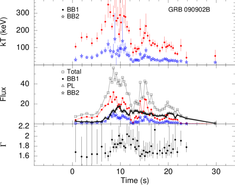
Figure 14: The evolution of the parameters as found by time-resolved spectral study of GRB 090902B using the 2BBPL model. The parameters are — (upper panel): temperature ($kT$) of the two BBs ; (second panel): flux (in the units of $10^{-6}$ erg cm^-2 s^-1) for the total (open boxes), BB1 (red filled circles), BB2 (blue stars), and PL (triangles joined by thick line); (bottom panel): power-law index ($\Gamma$). Source: Rao et al. (2014).

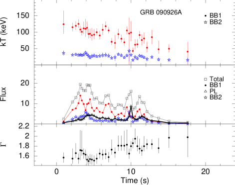
Figure 15: The evolution of the parameters as found by time-resolved spectral study of GRB 090926A using 2BBPL model. The symbols are the same as in Figure 14. Source: Rao et al. (2014).

3 Features Of Spectral Evolution

In Figure 14, and Figure 15, we have shown the evolution of various parameters for GRB 090902B and GRB 090926A, respectively. In the upper panel, we plot the evolution of $kT$ of the two BBs (BB1 and BB2). We note that $kT$ of the two BBs vary in a similar manner. In the second panel, we show the flux evolution of the total (grey open boxes), BB1 (red circles), BB2 (blue stars), and PL component (black triangles joined by thick line). We note the followings: (i) Evolution of $kT$ of both the BBs track the total flux evolution (or possibly the evolution of the respective BB flux), (ii) The flux evolution of the two BBs are similar to each other, and (iii) the PL component starts with a delay, and in GRB 090902B, the PL component lingers at the later phase. All these evolutions will be discussed in detail when we propose a simplistic model in chapter 6.

In the lowest panel, we have shown the evolution of $\Gamma$ of 2BBPL model fit. Note that the negative values of $\Gamma$ are shown for convenience. We note that the value is always lower than -3/2, the line of death of synchrotron emission from fast cooling electrons.

In Figure 16, we have studied the correlation between $kT$ (left panels) and normalization (right panels) of the two BBs of 2BBPL model. The upper panels show the data obtained for GRB 090902B, and the lower panels are those for GRB 090926A. We find high correlation in these parameters.

Figure 16: Correlation study between different parameters of 2BBPL model. For GRB 090902B, (A1): correlation between temperature ($kT$) of the two BBs, (A2): correlation between the flux of the two BBs. Similar plots for GRB 090926A are shown in (B1) and (B2). Source: Rao et al. (2014).

10 Summary

Before moving to the next chapter, let us summarize the results of the parametrized joint fit as applied to the brightest GRBs in the Fermi era. For the GRBs with separable pulses, we have seen that the spectrum has a photospheric origin, which is gradually taken over by a synchrotron emission. However, the photon index of the Band function is only within the slow cooling regime of the synchrotron emission. As we expect a GRB spectrum in the fast cooling regime, it is possible that though the synchrotron becomes important in the later phase, the spectrum is still not fully synchrotron. The models like mBBPL and 2BBPL have a more physical PL index ($\Gamma$). Hence, the spectrum is likely to be a combination of a thermal and a non-thermal component in general. Note that the same conclusion was obtained for the GRBs with single pulses.

By parametrization and tying scheme applied to all the models, we have arrived at the conclusion that the 2BBPL model is marginally preferred over all the other models in all episodes. We have found consistent results for GRB 081221 and GRB 090618, the two brightest Fermi GRBs with multiple broad pulse structures. It is unlikely that the results obtained for these two brightest cases can get any better for other GRBs.

For GRBs with high flux, but rapidly varying LC, we have performed our new technique by dropping the parametrization scheme. We obtain consistent results for three GRBs. Specially for GRB 090902B, we find that the instantaneous spectrum is far from being a Band function. The residual of a BBPL fit gives a clear indication of another BB. A fit with 2BBPL model gives an average $\chi^{2}_{\rm red}=1.05$, which is even better than a mBBPL model fit ($\chi^{2}_{\rm red}=1.14$). We want to emphasize here that the 2BBPL model is found either comparable or preferred than the other models for all cases where we have high signal to noise. Though we do not rule out the possibility that each GRB spectrum can be unique, however, the applicability of a single functional form to a diverse group (single/separable/multiple pulses) possibly indicates that a fundamental radiation process prevails in all GRBs in general.

Chapter 6 Predictions And Physical Picture

1 Overview

In the last two chapters, we have used various alternative models to describe the time evolution of the prompt emission spectrum, which spans a few keV to $\sim 10$ MeV energy band. We have extensively studied these models for the brightest GRBs detected by the Fermi/GBM. In addition to the prompt keV-MeV emission, GRBs are also accompanied by high energy (GeV) emission. CGRO/EGRET was the first instrument used for detecting GeV photons from GRBs. Though the detector severely suffered from backsplash (chapter 2), EGRET was quite successful in detecting a few GRBs with GeV emission. In the modern era, Large Area Telescope (LAT) of Fermi is providing a wealth of data for this class of GRBs. Through extensive studies by the LAT, it is now established that compared to the prompt keV-MeV emission, GeV emission has a delayed onset during the prompt emission phase, and has a longer lasting emission extending to the early afterglow phase. The time evolution of the GeV flux after the prompt emission shows a remarkable similarity with the x-ray and optical afterglows. In fact, it is suggested that GeV photons are produced via synchrotron emission in the external forward shock (Kumar & Barniol Duran 2010). However, this emission as early as the prompt emission is rather puzzling. More curious is the fact that the GeV emission is prominent in some of the brightest GRBs, while there is apparently very little GeV flux in others with comparable brightness in keV-MeV energies. In this chapter, we shall attempt to address some of the observations of GeV emission based on our knowledge of the prompt spectral evolution in the keV-MeV energy band.

Apart from the analysis of high energy spectral data, it is interesting to study the low energy x-ray spectrum ($\lesssim 10$ keV) during the early afterglow phase, and connect it with the prompt emission. However, it is difficult, as unlike the prompt $\gamma$-ray emission which is many orders higher than the background and readily triggers the open (or, large field of view) $\gamma$-ray detectors, x-rays are background limited and need to be focused. Hence, it takes a considerable time to relocate the burst with a focusing x-ray detector. The X-Ray Telescope (XRT) on-board Swift is a dedicated instrument for studying x-rays from a very early stage of the GRB afterglow phase (chapter 2). The XRT has established a canonical picture of the x-ray afterglow with various breaks in the lightcurve. It is suggested that the rapid flux decay before the shallow phase of x-ray afterglow is possibly an after-effect of the late phase of the prompt emission. If it is true, the spectral parameters of the prompt emission should smoothly join those of the early XRT data. By extending the evolution of the prompt emission model, we shall try to connect these two regimes.

The first topic of this chapter is to obtain some predictions for the emission characteristics of the highest energy $\gamma$-rays (GeV, Basak & Rao 2013a) as well as the low energy x-rays ($<10$ keV; Basak et al. in preparation) from the spectral model fitted to the prompt keV-MeV data (Part I and II). In the previous chapters, based on detailed analysis of the time-resolved spectra, we have found that a new model, viz. two blackbodies along with a power-law (2BBPL) is preferred over the other models. In this chapter, we shall assume this model for the keV-MeV spectrum and study how the components connect with the emissions in other wavelengths. We shall also show that none of the other models (Band, BBPL and mBBPL) can explain all the observations. In the third part of our discussion, we shall present a simplistic (and tentative) physical model for the origin of the 2BBPL model.

Part I: Predicting GeV Emission
From MeV Spectrum

2 Background

1 Features Of GeV Emission

Let us begin our discussion with the GeV emission in GRBs. The first long detection of GeV emission was found in GRB 940217 (Hurley et al. 1994) detected by CGRO/EGRET. The GeV emission continued for 90 minutes after the trigger, which showed the longer lasting behaviour of GeV emission. However, with the EGRET and the LAT data it is clear that GeV emission is not solely an afterglow component, it appears during the prompt emission phase, sometimes starting with a delay, and showing the major bursting features of the prompt keV-MeV emission save for the initial phase in some cases. In this regard, the GeV emission behaves like a “bridge” between the prompt and the afterglow emission. Hence, it is interesting to study the GeV emission in light of the evolution of the prompt keV-MeV emission.

In addition to the unique lightcurve (LC), the spectrum of GeV emission is also interesting, and shows diverse features. For example, Dingus et al. (1998) have found a consistent fit for the wide-band spectral data using a Band function, while González et al. (2003) have found an additional PL component which becomes progressively important at a later phase. Recent observations with the Fermi/LAT has validated these observations. With a good sample size (currently 35; Ackermann et al. 2013), the delayed emission, longer lasting behaviour and addition spectral component are found in many cases (Abdo et al. 2009b, c, Ackermann et al. 2010b, Kumar & Barniol Duran 2009, 2010, Barniol Duran & Kumar 2011, Ackermann et al. 2013). In the following, we shall briefly describe the current understanding based on the comparative study of the GBM and the LAT data. For convenience of description, we shall interchangably use the “GeV” emission with the “LAT” emission (and similarly the “keV-MeV” emission with the “GBM” emission).

2 GBM-LAT Correlation

The Fermi/LAT is the modern dedicated instrument for studying GeV emission (see chapter 2 for details). Recently, Fermi LAT team (Ackermann et al. 2013, A13 hereafter) have published the first catalogue of GRBs detected by the LAT (also see Granot et al. 2010, Akerlof et al. 2011, Rubtsov et al. 2012). In order to establish a possible connection between the prompt keV-MeV and GeV emission, A13 have studied the GBM and the LAT fluence in the “GBM time window”. The LAT fluence is calculated by independently fitting the GBM-LAT data and the LAT-only data. For bright bursts, the two fits disagree in the LAT energy band due to the presence of multiple spectral components in the GBM-LAT joint data. In order to account for the longer lasting behaviour of GeV emission, they have also calculated the GeV fluence in the “LAT time window”. They have studied the relative fluence in the GBM and the LAT between 19 GRBs (17 LGRBs), and have found only a tentative correlation, i.e., GRBs with high keV-MeV emission are likely to produce high GeV emission. In fact, for off-axis GRBs from the LAT field of view, the current strategy of the LAT observation is to re-point the telescope to a GRB with high GBM flux. However, the correlation data of A13 has a large scatter, e.g., GRBs with similar GBM fluence are found to have widely different LAT fluence. In fact, A13 have categorized the GRBs into two classes, namely, hyper-fluent LAT bursts (GRB 090902B, GRB 090926A, GRB 080916C, and GRB 090510), and the rest. In an attempt to find a correlation between the GBM and the LAT emission components, Zheng et al. (2012, Z12 hereafter) have selected a sample of 22 GRBs (17 LGRBs). Since the LAT photons are either simultaneous or delayed than the GBM emission, they have selected a uniform 47.5 s time window of match filter technique for both the emissions. The LAT emission outside this time window is considered to be much delayed, and unusable for a correlation study. For the LGRB sample, Z12 also find a weak correlation with a Pearson correlation coefficient, $r=0.537$.

The lack of a strong connection between the GeV and keV-MeV emission could be a manifestation of spectral diversity of the prompt emission. In the standard model, though the basic ingredients are roughly known, the subsequent emission strongly depends upon the unknown initial conditions e.g., emission region, the amount of energy shared by the magnetic field, and the baryon loading of the ejecta (Mészáros 2006). For example, Zhang et al. (2011) have analyzed the broadband data of a set of 17 GRBs. They have found five possible combination of the spectral models (a combination of Band, BB, PL etc). Models other than a Band only function is found for the brightest GRBs. In the following we shall try a single model to describe all the GRBs, and hope for a better GBM-LAT correlation.

Figure 1: Lightcurve of GRB 080916C in various energy bands. The GeV emission detected in the LAT is delayed by $\sim 4$ s from the keV-MeV emission detected in the GBM.

3 Sample Selection And Analysis Method

The A13 catalogue has used 17 LGRBs for studying the GBM-LAT fluence correlation. Among these, 5 GRBs have either much delayed the LAT emission than the GBM emission, or only an upper limit of the GBM and/or the LAT fluence. The Z12 catalogue ignores the following GRBs — 090323, 090328, 090626, 091031, and 100116A, and adds the following GRBs — 091208B, 100325A, 100724B, 110709A, and 120107A. As we are interested in finding a connection between the GBM and the LAT emission during the prompt emission, we follow the uniform time selection criteria of Z12, and study all the GRBs in their sample.

Note that our aim is to perform a spectral fit to the GBM data without invoking the LAT data, and investigate whether any spectral component can predict the LAT observation. As a Band only function does not give a strong correlation, we choose a model having a thermal and non-thermal component, which hopefully gives a better understanding of the physical process. As we have found that the 2BBPL model gives either comparable or marginally better fit to a variety of data, it is interesting to apply this model. Hence, we use 2BBPL model to fit the GBM spectrum of all GRBs with GeV emission. In the previous chapter, we have developed the “parametrized-joint fit” technique (Basak & Rao 2013b) for spectral analysis of GRBs with separable pulses. However, note that majority of the bursts in our present sample do not have well-defined broad pulse structure. Hence, we drop the parametrization scheme in order to perform uniform spectral fitting for all the bursts. However, we tie the PL index ($\Gamma$), and the ratio of the temperatures ($kT$), and normalizations ($N$) of the two BBs. We extract the time-resolved bins by requiring $C_{\rm min}$ between 800-1200, which is chosen by considering the peak flux and duration. For GRBs with high GBM flux (GRB 090902B, GRB 090926A, and GRB 100724B), we choose a higher value of $C_{\rm min}$ ($1800-2000$). For GRB 081006, which has a low GBM count, we use only one bin covering the entire burst (-0.26 to 5.9 s; see A13).

Figure 2: Lightcurve of GRB 090902B in various energy bands. The GeV emission is delayed by $\sim 3$ s from the keV-MeV emission.

We calculate the flux value of each component of 2BBPL model in each time bin. The error of normalization is scaled to calculate the error in flux of each of the components. All these values are used to calculate the fluence and the corresponding error of each component and the total model. For the LAT analysis, we use LAT Science Tools-v9r33p1 package, choosing “transient class” response function (see chapter 2 for detail). The LAT fluence (event count) is directly taken from Z12. Note that Z12 provide the LAT fluence in a 47.5 s time window. We determine the GBM fluence both in $T_{90}$ duration (as provided by A13), and within the 47.5 s inetrval. We study both Spearman rank (coefficient $\rho$, and chance probability $P_{\rho}$) and Pearson linear correlations (coefficient $r$, and chance probability $P_{\rm r}$). We study the correlation of the LAT fluence with both the total, and the PL component of the GBM fluence. In order to determine which among these correlations is more fundamental, we perform Spearman partial rank correlation test (Macklin 1982). This method finds the correlation of two variables, say A and X, when a third variable (Y) is present. The confidence level that the A-X correlation is unaffected by X-Y correlation is given by the D-parameter, whose value should be at least -1 for a significant correlation. The relation between the two fluence quantities are found by fitting a linear function to the logarithmic values, and assuming a Gaussian noise ($\sigma_{\rm int}$), denoting an intrinsic scatter of the data (see chapter 3).

4 Analysis Of GRBs With High GeV Emission

1 Delayed Onset Of The LAT Lightcurve

In chapter 5, we have done a detailed time-resolved spectroscopy of three bright GRBs with high GeV emission, namely, GRB 080916C, GRB 090902B, and GRB 090926A. These bursts are classified as the hyper-fluent LAT GRBs (A13). Here, we shall discuss about the essential features relevant to find a relation between the low energy (GBM) and high energy (LAT) emission. In Figure, 1 (GRB 080916C), 2 (GRB 090902B), and 3 (GRB 090926A), we have shown the LC of these GRBs in three energy bands: $8~{}{\rm keV}-260~{}{\rm keV}$, 260 keV-5 MeV, and $>100$ MeV. Note that in all cases the LAT emission is delayed compared to the prompt emission in the GBM. The Fermi LAT team reports the following delay of the LAT emission: 4 s (GRB 080916C, Abdo et al. 2009c), 3 s (GRB 090902B, Abdo et al. 2009b), and 5 s (GRB 090926A, Ackermann et al. 2011). In chapter 5, we have fitted the time-resolved data of GRB 090902B and GRB 090926A with 2BBPL model. We have found that the two BBs of the 2BBPL model trace each other, while the PL component has a delayed onset (see Figue 14, and 15). Hence, we suspect that the PL component might be connected with the LAT emission. If they are indeed connected the evolution of the PL flux of the keV-MeV data should be similar to the LAT flux. Also, the total flux in the PL component, rather than the total flux of the GBM spectrum should show a better correlation with the total LAT flux.

Figure 3: Lightcurve of GRB 090926A in various energy bands. The GeV emission is delayed by $\sim 5$ s from the keV-MeV emission.

2 Evolution Of The Power-law Flux

We first perform a comparative study of the evolution of the PL flux and the LAT flux. In addition to the time-resolved bins in the main bursting phase, we use a few large time bins at the late stage of the prompt emission for our study. These time bins are: 25-30 s, 30-40 s, 40-60 s, and 60-100 s (for GRB 090902B); 17-30 s, 30-50 s, 50-70 s (for GRB 090926A), and 64-100 s (for GRB 080916C). We fit a power-law to the broad bin GBM data of each GRB, with an index frozen at the average value of that we find during the burst. In the following, we investigate whether the PL flux in the GBM spectrum (which is presumably the non-thermal component of the spectrum) is related with the LAT count (which we assume to have a non-thermal origin).

Figure 4: Comparison of the power-law (PL) flux with the LAT photon flux. (Left panels): The evolution of PL flux (in units of $10^{-6}$ erg cm^-2 s^-1) as calculated by the time-resolved spectroscopy with 2BBPL model (open squares). The LAT count flux (in the units of LAT count rate for $>100$ MeV events) is marked by stars. (Right panels): The cumulative integrated flux distribution of the GBM PL flux (open symbols) compared to that of the LAT count flux (corresponding filled symbols). The GRBs are (top to bottom) GRB 090902B, GRB 090926A, and GRB 080916C. Source: Rao et al. (2014),

Figure 4 (left panel) shows the evolution of the non-thermal GBM flux (open boxes) in the units of $10^{-6}$ erg cm^-2 s^-1, and the LAT flux (stars) in the units of LAT count rate in the $>100$ MeV energies. It is quite fortuitous that our choice of units makes the values of these quantities in the same range. As the LAT bore-sight angle is almost similar for these GRBs, namely, $49^{0}$ (GRB 080916C), $50^{0}$ (GRB 090902B), and $47^{0}$ (GRB 090926A), the observed LAT flux can be regarded as the relative flux of a given GRB. It is clear from this figure that the flux of the PL component of the GBM and the LAT flux track each other quite well. For GRB 090902B, for example, we have found that the PL flux is $\approx 1$ order of magnitude lower than the total flux in the initial $\sim 6$ s data (Figure 14). This evolution coincides with the rise of the LAT flux quite smoothly. The peaks near 9-11 s also coincide, though the PL flux decays faster than the LAT after 20 s. This probably denotes the “end” of the prompt emission. But, quite remarkably the LAT emission enters into the afterglow phase. For GRB 090926A, the PL flux is delayed compared to the total flux by $\sim 3$ s, which is comparable to the delay of the LAT ($\sim 5$ s). The sharp drop of the PL flux is noted at the end. For GRB 080916C, the flux evolutions track each other, including a dip near $\sim 55$ s. In the right panel of Figure 4, we have shown the cumulative flux distribution which again highlights the similarity between the flux evolution of the LAT and the PL component of the GBM spectrum. From the above discussions, we infer that the PL flux has a similar behaviour as the LAT flux both in terms of delayed onset and long-lived emission.

Figure 5: A scatter-plot of the PL flux of 2BBPL model with the LAT count rate for the time-resolved spectral analysis. The GRBs are GRB 090902B (stars), GRB 090926A (open squares), and GRB 080916C (open circles). Source: Rao et al. (2014).

In Figure 5, we have shown a scatter-plot of the PL flux of the GBM versus the LAT count rate flux as obtained in the time-resolved study of these GRBs. Though the correlations obtained for GRB 090926A ($r=0.32$), and GRB 080916C ($r=0.36$) are weak, for GRB 090902B, we obtain a strong correlation ($r=0.84$) between these two emissions.

5 Comparison Of Hyper-fluent With Low-LAT Class

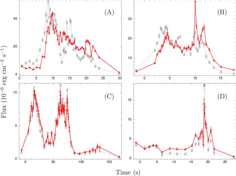
Figure 6: The evolution of the total flux (diamonds joined by dashed line), and the non-thermal (power-law) flux (pluses joined by solid line) is shown for two category of GRBs in our sample. (upper panels): GRBs with high GeV emission as detected by the LAT. The GRBs are (A) GRB 090902B with 378.1 photons m^-2 LAT count, and (B) GRB 090926A with 372.2 photons m^-2 LAT count. (lower panels): GRBs with similar GBM fluence, but with much lower GeV fluence. The GRBs are (C) GRB 100724B with 23.9 photons m^-2, and (D) GRB 091003 with 14.8 photons m^-2. The values of fluence are calculated in 47.5 s time window. Note the delayed onset and lingering behaviour of the PL component for the first category (see text). Source: Basak & Rao (2013a).

It is evident from our discussion of the hyper-fluent GRBs that their associated LAT photons are delayed, and so is the PL component of the prompt keV-MeV emission. This behaviour seems to be ubiquitous for the hyper-fluent LAT GRBs. The natural question that arises is “how does the LAT and PL emission evolve for GRBs with low LAT count”? In order to address this question let us choose a few sample GRBs. Note that Z12 have found a weak but a definite correlation between the GBM and the LAT fluence (Figure 5 of Z12). That is, we expect high LAT count only for GRBs with high GBM count. Hence, we should choose GRBs with comparable GBM fluence. A quick look at Figure 5 of Z12 clearly shows two classes of our interest — (i) GRBs with high GBM fluence as well as high LAT fluence (hyper-fluent LAT class), and (ii) GRBs with the same order of magnitude GBM fluence, but an order of magnitude lower LAT fluence. From set (i), we choose GRB 090902B, and GRB 090926A. From set (ii) we choose GRB 100724B, and GRB 091003. Among the class (ii) GRBs, GRB 100724B has a fluence similar to GRB 090902B, and even greater than GRB 090926A, but a very low LAT fluence of $23.9\pm 7.6$ photons m^-2 (compared to $378.1\pm 29.5$ photons m^-2 and $372.2\pm 28.0$ photons m^-2 for GRB 090902B and GRB 090926A, respectively). GRB 091003 has a factor of 5 lower GBM fluence, but a factor of 25 lower LAT fluence ($14.8\pm 4.5$ photons m^-2) than GRB 090902B.

In Figure 6, we have shown the evolution of the total GBM flux (diamonds joined by dashed line) along with the flux of the PL component (pluses joined by solid line). To show both the evolutions in the same scale, we have multiplied the PL flux by a constant, which is the ratio of the average GBM flux and average PL flux. The upper panels show the evolutions for GRBs with high LAT count, while the lower panels show those for the low-LAT GRBs. Clearly, the non-thermal component of each high-LAT GRB has a delayed onset, and this component lingers at the later phase of the prompt emission. The low-LAT GRBs apparently show no such trend. For this class, the PL component starts simultaneously, and traces the total GBM flux.

A quick look at Figure 2 and 3 immediately shows that the evolution of the LAT flux of the two high-LAT GRBs have a similar characteristic as the PL flux evolution. The LAT flux also starts with a delay and lingers later (A13). Note that we have fitted only the GBM data with a model consisting of a thermal and a non-thermal component, without invoking the LAT data. Still the evolution of the PL component of the keV-MeV data alone shows this remarkable similarity with the LAT flux evolution (see LAT Low-Energy (LLE: 30-100 MeV) lightcurve in Figure 59, 61 of A13 for GRB 090902B and GRB 090926A, respectively). On the other hand, a look at the LLE lightcurves in Figure 63 (GRB 091003) and 78 (GRB 100724B) of A13 shows that the LAT photons (low energy) do not have a delay. Hence, we conclude that (i) the PL component of the 2BBPL model mimics the evolution of the LAT flux in the low energy GBM data, and (ii) GRBs with a delayed and lingering PL component are likely to be LAT-bright.

Table 1: The GBM and LAT fluence of the 17 GRBs with GeV emission

GRB	GBM $T_{90}$ window(a)		47.5 s time window		LAT fluence
	(Photon cm-2)		(Photon cm-2)		(Photon m-2)
	Total fluence	PL fluence	Total fluence	PL fluence	in 47.5 s
080825C	224.8$\pm$6.2	105.2$\pm$5.5	245.1$\pm$13.3	115.7$\pm$11.9	36.6$\pm$11.6
080916C	369.9$\pm$7.7	223.9$\pm$6.4	329.3$\pm$5.7	196.34$\pm$4.8	279.0$\pm$24.9
081006A(b)	6.97$\pm$0.92	3.24$\pm$0.62	6.97$\pm$0.92	3.24$\pm$0.62	16.3$\pm$4.7
090217	124.7$\pm$4.1	54.1$\pm$3.4	129.0$\pm$4.4	55.8$\pm$3.7	22.5$\pm$6.0
090902B	1028.4$\pm$18.6	498.3$\pm$14.6	1102.7$\pm$29.6	525.3$\pm$23.2	378.1$\pm$29.5
090926A	739.6$\pm$10.8	324.9$\pm$8.6	785.6$\pm$13.1	343.3$\pm$10.4	372.2$\pm$28.0
091003	186.8$\pm$6.3	95.9$\pm$4.6	210.1$\pm$9.8	107.7$\pm$7.2	14.8$\pm$4.5
091208B	60.5$\pm$3.5	37.2$\pm$3.1	82.5$\pm$11.4	43.6$\pm$10.0	14.6$\pm$6.5
100325A	13.4$\pm$1.7	3.3$\pm$0.9	13.9$\pm$1.7	3.6$\pm$0.9	6.7$\pm$3.0
100414A	289.9$\pm$7.6	103.4$\pm$6.2	384.8$\pm$7.9	145.4$\pm$6.4	87.5$\pm$33.1
100724B	998.5$\pm$9.5	500.6$\pm$7.1	396.6$\pm$3.8	212.4$\pm$2.9	23.9$\pm$7.6
110120A	69.1$\pm$4.7	27.5$\pm$2.2	77.9$\pm$7.2	32.6$\pm$3.4	9.5$\pm$3.6
110428A	127.4$\pm$3.5	32.4$\pm$2.6	147.6$\pm$5.5	44.0$\pm$4.0	8.0$\pm$3.6
110709A	198.9$\pm$5.6	92.2$\pm$5.2	212.1$\pm$6.2	101.1$\pm$5.7	18.7$\pm$7.1
110721A	182.2$\pm$7.2	98.8$\pm$4.5	192.5$\pm$9.6	105.0$\pm$6.0	46.4$\pm$9.3
110731A	89.6$\pm$5.7	55.5$\pm$2.0	102.9$\pm$11.9	66.9$\pm$4.1	81.5$\pm$10.4
120107A	39.5$\pm$4.1	25.8$\pm$4.9	39.7$\pm$5.2	25.8$\pm$3.9	17.6$\pm$7.2

6 A Detailed Correlation Analysis

From the analysis of the previous section (5), it follows that the PL component of the 2BBPL model has some close relation with the LAT emission. In section 2, we have seen that the non-thermal flux of the time-resolved data of hyper-fluent GRBs indicates a correlation with the LAT flux. However, a flux correlation suffers from the fact that the LAT flux has a delay compared to the corresponding GBM flux. Hence, choosing similar bins for the LAT and the data GBM may wipe out the correlation. Since it is not clear whether the GeV emission is derived from the MeV emission, it may not be possible to correct for the delay. Hence, a correlation study between the fluence quantities seems more reliable. As in this case, we integrate the flux over a chosen time window, it suffers from little error (only contribution, if any, comes from the delayed onset). Both A13 and Z12 have studied fluence correlation rather than flux correlation. Also note that the total fluence in “LAT time window” may not be used for the following reason. We have already seen that the PL flux decreases sharply during the late prompt emission phase, while the LAT emission survives. An extended LAT emission is probably an afterglow phenomenon, rather than a prompt emission. By choosing a time window in the prompt emission phase, we are effectively extracting only the prompt contribution of the LAT data. Following Z12, we use the 47.5 s data from the trigger time of the GBM. However, as the boundary of the late prompt and early afterglow phase is rather arbitrary, the choice of the time window is not unique.

Figure 7: Correlations between the GBM photon fluence (photons cm^-2) and the LAT photon fluence (photons m^-2). The values of fluence are calculated in 47.5 s time window. (Left panel): Correlation of the total GBM fluence with the LAT fluence, (Right panel): correlation of non-thermal GBM fluence with the LAT fluence. Source: Basak & Rao (2013a).

In our analysis, we perform two kinds of correlations: I — the LAT fluence with the total GBM fluence, II — the LAT fluence with the fluence of the non-thermal (PL) component. The GBM fluence is calculated both in the GBM $T_{90}$, and in the 47.5 s time window (Z12). We designate the former with ‘a’, and the latter with ‘b’. In Table 1, we have shown the sample of GRBs we have analyzed (Z12 sample of LGRBs). We have shown the total and the PL fluence of the GBM in the two time windows. The values of the LAT fluence is shown in the last column (taken from Z12).

In Figure 7, we have shown the data for the LAT-Total GBM fluence correlation (Ib, left panel) and the LAT-PL GBM fluence correlation (IIb, right panel) cases, as described above. The correlation coefficient of these cases are reported in Table 2 (last two rows). The $p$-values of the correlations are low, denoting that the correlations are not due to chance. We note that the correlation using $T_{90}$ time window (first two rows) are inferior to those using the 47.5 s time window. This suggests that a uniform time window is a better choice. Also, note that the correlation of the total GBM fluence (in $T_{90}$) with the LAT fluence (0.68) is better than the Z12 correlation (0.537). This is possibly due to the different spectral models as well as different values of $T_{90}$.

The correlation of Ib ($r=0.87$) and IIb ($r=0.88$) are comparable in terms of the Pearson linear correlation. Using the logarithmic values, the corresponding coefficients are 0.68 and 0.72, respectively. We now use the Spearman partial rank correlation to find out which is the more fundamental correlation. The coefficient are $\rho=0.75$ and $\rho=0.81$ for Ib and IIb cases, respectively. Note that a Spearman correlation does not assume the linearity of data, and hence it is a more robust estimator of the correlation (Macklin 1982). Also, the outliers have least effects on the correlation i.e., if some GRBs are really exceptional, while others follow a trend, then a Spearman rank is more reliable. Note that the correlations using $T_{90}$ time window have comparable $\rho$ to the corresponding cases using 47.5 s time window. We calculate the $D$-parameter of I and II correlation. For a 47.5 s time window, we see that a correlation of the LAT fluence with the total GBM fluence (Ib) has $D=-1.4$, while the correlation of the LAT fluence with the non-thermal GBM fluence (IIb) has $D=2.3$. Hence, based on the $D$ value, we conclude that the correlation between the LAT and the non-thermal GBM fluence exists in the presence of a third parameter, namely the total GBM fluence, and it is the more fundamental correlation. Using the fluence values in $T_{90}$ instead of 47.5 s window leads to similar conclusions.

If we assume that the fluence are related as a power-law function, then we can fit a linear function to the logarithmic data as: ${\rm log}(y)=K+\delta{\rm log}(x)$, where $y$ is the LAT fluence, and $x$ is either the total GBM fluence or the PL fluence. In Table LABEL:ch6_t3, we have shown the best-fit parameters $K$, $\delta$, and $\sigma_{\rm int}$. Note that the values of the slopes are remarkably similar, denoting that high PL fluence is expected for high total fluence, and either of them acts as a proxy of high LAT fluence. However, based on the value of $D$-parameter, the PL fluence is a better indicator of the LAT fluence. Note that the $\sigma_{\rm int}$ has a lower value for IIb case, which again shows that the LAT-PL GBM fluence correlation is “better understood” than the LAT-total GBM fluence correlation.

Table 2: Correlations between (i) the LAT fluence with the GBM fluence, and (ii) the LAT fluence with the GBM PL fluence

Correlation	Pearson		Spearman
	r	$\rm P_{r}$	$\rho$	$\rm P_{\rho}$	$D$
Ia	0.68	$2.67\times 10^{-7}$	0.73	$8.20\times 10^{-4}$	-0.6
IIa	0.68	$2.67\times 10^{-7}$	0.79	$1.66\times 10^{-4}$	1.8
Ib	0.87	$5.66\times 10^{-6}$	0.75	$5.61\times 10^{-4}$	-1.4
IIb	0.88	$3.20\times 10^{-6}$	0.81	$9.23\times 10^{-5}$	2.3

Table 3: Results of linear fit to the correlation data in Figure 7

Correlation$\rightarrow$	GBM-LAT (Ib)	GBM PL-LAT (IIb)
$K$	$0.056\pm 0.099$	$0.288\pm 0.096$
$\delta$	$0.698\pm 0.044$	$0.697\pm 0.049$
$\sigma_{int}$	$0.385\pm 0.084$	$0.368\pm 0.081$
$\chi^{2}_{red}$ (dof)	1.10 (15)	1.10 (15)

7 Summary And Discussion On GeV Prediction

1 The Correlation

To summarize, we have used a model consisting of a thermal and a non-thermal component to fit the time-resolved GBM data of GRBs, which have GeV emission during the prompt emission phase. The thermal component of our model is represented by two correlated BBs, and the non-thermal component is assumed as a PL. We have found that a spectral fit using only the GBM data has a predictive power for the LAT emission. For example, the fluence of the PL component bears a strong correlation with the GeV fluence. Previous attempts to find such a connection between keV-MeV emission and GeV emission have failed in a sense that (i) no unified spectral model is found, and (ii) correlation using Band only function (as used by Z12) is weak. The reason behind the success of our study lies in segregating the thermal and non-thermal components of the prompt emission data, and using only the non-thermal component to investigate the correlation.

We would like to point out that a mBBPL model is likely to show similar improvement over a correlation, which is studied through a Band only fitting. We have seen that the data of some GRBs are indeed consistent with a mBBPL model, e.g., GRB 090902B (Ryde et al. 2010). However, a 2BBPL model also gives a comparable fit. It is worthwhile to mention that several recent studies indicate that the prompt emission data of some GRBs require a separate thermal component, rather than a continuous distribution of temperature (Guiriec et al. 2011, Axelsson et al. 2012). For example, Guiriec et al. (2011) find a sub-dominant BB with a temperature, $kT\approx 38$ keV, along with a Band function with $E_{\rm peak}\approx 350$ keV. Note that the peak energy corresponds to a $kT\approx 117$ keV, which has a temperature ratio $\sim 3$ with the lower BB. This ratio is of the same order we find for many GRBs. Can we use BB+Band function for the correlation study? A BB+Band model fit to the data cannot give a possible connection between the non-thermal (Band function) and GeV photon for the following reason. We have explicitly shown for GRBs with high GeV count that the PL of 2BBPL model is delayed and mimics the GeV flux evolution, whereas the two BBs are correlated and do not have any delay (Figure 13 and 14). Using a BB+Band function for such bursts will replace the higher BB peak with a Band peak, and the corresponding flux will not show a delay. Incidentally, GRB 100724B, which is fitted with BB+Band, is included in our LAT sample, and the data is consistent with a 2BBPL model. It is worthwhile to emphasize again that the 2BBPL model stands out as a universal model for time-resolved GRB spectrum, and the non-thermal component of this function gives a better insight for GeV emission.

2 Constraining Physical Models

The origin of the GeV emission is still a matter of intense debate (e.g., Meszaros & Rees 1994, Waxman 1997, Gupta & Zhang 2007, Panaitescu 2008, Fan & Piran 2008, Zhang & Pe’er 2009, Mészáros & Rees 2011). Majority of the mechanisms to produce GeV photons during the prompt and afterglow phase involve inverse compton (IC) of some seed photon. Zhang (2007b) has listed many possible sites of IC including self-Compton in internal and external shock. For example, (i) synchrotron self-Compton (SSC) by electrons accelerated in the IS (e.g., Meszaros et al. 1994, Pilla & Loeb 1998, Razzaque et al. 2004, Pe’er & Waxman 2004b, 2005, Pe’er et al. 2005, 2006), (ii) Synchrotron emission from accelerated protons or photon-meson interaction in the IS (Totani 1998, Bhattacharjee & Gupta 2003), (iii) SSC in the ES — (a) forward shock (Meszaros & Rees 1994, Dermer et al. 2000, Panaitescu & Kumar 2000, Zhang & Mészáros 2001, Kumar & Barniol Duran 2009, 2010), (b) reverse shock (Wang et al. 2001a, Granot & Guetta 2003), and (c) cross IC of photons in either region (Wang et al. 2001a, b), (iv) IC of prompt keV-MeV photons in the ES (Beloborodov 2005, Fan et al. 2005), (v) IC of photons from x-ray flare in ES (Wang et al. 2006, Fan & Piran 2006), or SSC of x-ray flare photons (Wang et al. 2006), and so on. It is important to identify the correct mechanism, as it can give additional constraint on the unknown fireball parameters. For example, Gupta & Zhang (2007) have shown that for a $\epsilon_{\rm e}$ (fraction of energy carried by electrons) not too low, the leptonic models are preferred. Hence, synchrotron emission from protons or photon-meson interaction is disfavoured for high energy (GeV) emission.

The observation of GeV emission can help in constraining the possible models of prompt emission. If we assume, e.g., an IS origin, and extrapolate the Band function fitted to the prompt keV-MeV data, then it generally over-predicts the GeV emission in the LAT (Le & Dermer 2009). It is shown that a low detection rate of the LAT is consistent with a ratio of GeV to MeV emission $\sim 0.1$ (however, see Guetta et al. 2011). Beniamini et al. (2011), using 18 bright GRBs with no LAT detection, have found an upper limit of the fluence ratio $\sim 0.13$ (during the prompt emission phase), $\sim 0.45$ (during 600 s time window). These ratios put a strong constraint on the possible prompt emission model, and particularly rules out SSC for both MeV and GeV data. The implication of our finding in the comparative study of the GBM and the LAT data is that only the PL component is connected with the GeV emission. If the photospheric emission is efficient, the 2BBs possibly do not have any connection with the GeV emission. This requirement puts more constraints on the GeV afterglow model. For example, if we consider SSC as the possible mechanism, then the circumburst density required to explain GeV emission for usual values of parameters varies as some negative power of the energy (Wang et al. 2013). As the energy is channelized into two components, the required density increases. For bursts like GRB 090902B, which have a low calculated circumburst density from afterglow modelling (e.g., Liu & Wang 2011), SSC becomes quite impossible.

3 Spectral Break Or Cut-off

One of the most important application of GeV emission is to give a lower limit on the unknown bulk Lorentz factor ($\Gamma$, Woods & Loeb 1995, section 1.5.1). While $\Gamma$ can be estimated from the variability time scale, observation of the highest GeV photon provides an independent measurement. Note that none of these provide an accurate measurement, and hence, it is important to have such independent estimators. It is expected that the spectrum at very high energy should have a cut-off due to the photon-photon interaction. As this cut-off directly depends on $\Gamma$, observation of cut-off gives another measurement of $\Gamma$. It is also interesting to compare the spectral index of the MeV and GeV data to get an indication of spectral break or cut-off. In our analysis, we have computed the average spectral index of 2BBPL model fit for the hyper-fluent LAT GRBs. For GRB 090902B, the average spectral index in the GBM data ($-1.76\pm 0.17$) is remarkably consistent with that of the LAT data (also $-1.76$, Zhang et al. 2011), showing no cut-off. However, for GRB 090926A, the average index ($-1.65\pm 0.35$) is clearly inconsistent with that of the GeV data ($-2.03$). Hence, there is possibly a spectral break in the second case. A higher spectral slope can possibly indicate that the spectrum approaches a cut-off. Ackermann et al. (2011) have indeed found a cut-off in the spectrum during 9.7-10.5 s of this GRB.

4 Delayed Onset: Early Indication Of GeV Emission

Finally, the PL component in the GBM spectrum of the hyper-fluent LAT GRBs have shown delayed onset and lingering behaviour. GRBs with similar brightness, but an order of magnitude lower LAT count have a coupled PL and total GBM flux variation. In part III of this chapter, we shall discuss about the possible reason of this dual behaviour of PL in terms of a tentative model. We would like to mention that this delayed onset can be used as an early indication of high GeV emission. The current strategy for the off-axis LAT events is to target the brightest GRBs. Based on our analysis, it is evident that even moderately bright GRBs with a delayed PL component may be targeted. A combination of these two criteria can increase the number of GRBs detected by the LAT, and it can also shed light on the seemingly different characteristics of the LAT emission in GRBs with similar GBM brightness.

Part II: Predictions For Low Energy Data

We now turn our discussion to the predictions for the low energy data. We shall use the Swift/XRT for our purpose, and illustrate the predictions for two GRBs.

8 A Hypothetical Situation

Let us first assume a hypothetical situation based on our phenomenological understanding of 2BBPL model. In Figure 8, we have shown the evolution of the two BB temperatures ($kT_{h}$, and $kT_{l}$) as functions of “running fluence”. The evolution of $kT_{h}$ and $kT_{l}$ are shown as strictly hot-to-cold (LK96-like evolution). We expect such evolution for a GRB with a single smooth pulse. Note that, the “running fluence” is a monotonically increasing function of time. Hence, the evolution will be similar if we replace this quantity with time. As we have seen that the ratio of the two BB temperatures is $\sim 3-5$, it is possible that the lower BB goes below the lowest sensitive energy band of the higher energy detectors (GBM and BAT). Note that though the GBM has a lower energy coverage ($\sim 8$ keV) than the BAT ($\sim 15$ keV), we have found that the 8-15 keV band of GBM has $\lesssim 2-3\sigma$ count rate per bin. Hence, a spectral component below the lowest BAT energy is unlikely to be significantly detected in the GBM detector. For convenience of description, let us denote the lowest sensitive energy of these detectors as $E_{\rm low}$. The transition of $kT_{l}$ at $E_{\rm low}$ will have the following observational effects.

• (i) If we attempt to fit the spectrum of the GBM and/or the BAT data with a BBPL model, we shall get average $kT$ in the initial bins. As the lower BB is absent in the later bins of higher energy detectors, we expect a break during the transition of lower BB at $E_{\rm low}$ (see Figure 8). This break is expected to be smooth, as the higher part of the lower BB spectrum will have some residual effect during the transition. Note that, if the two BBs have their corresponding breaks, there can be a variety of averaging effects. In particular, the average temperature in the initial bins can show even an increasing temperature evolution.

• (ii) More interestingly, the lower BB can show up in the later XRT spectrum. Provided that the XRT data is available in the late prompt emission phase, this should be detectable. If this BB is indeed the lower BB of the initial time bins, the lower BB temperature, $kT_{l}$ as found by fitting 2BBPL model to the initial GBM and/or BAT spectrum should smoothly join with the $kT$ of the XRT data.

In the following, we shall look for these two observational effects. For the first effect to be seen, we require a GRB with single pulse and a break in $kT$ evolution (when fitted with a BBPL model). For the later effect, we require a GRB with long duration so that the XRT data is available in the final phase. For this kind of GRB, we shall look at the falling part of the final pulse, firstly because we expect a smooth cooling in the falling part, and second, only the last pulse is smoothly connected with the XRT observation, provided that the two observations overlap at all.

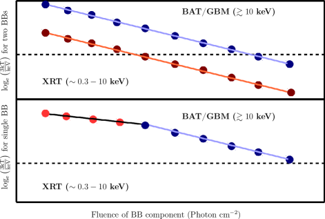
Figure 8: A hypothetical case: temperature ($kT$) evolution as a function of “running fluence” in a GRB with smooth single pulse. As the two $kT$ of two BBs evolve simultaneously, the lower BB can transit from the BAT/GBM lower range to the XRT band (upper panel). If one tries to fit BBPL the $kT$ will show a phenomenological break (lower panel). If the XRT data is available, the lower BB can be detected (see text).

Table 4: Parameters of linear fit to the fluence-log_e($kT$) data

Model	Intercept	Slope	$\chi^{2}$ (dof)
BBPL(a)	$3.02_{-0.29}^{+0.30}$	$(-4.56\pm 1.84)\times 10^{-2}$	0.46 (4)
2BBPL	$3.10_{-0.22}^{+0.23}$	$(-5.10\pm 1.48)\times 10^{-2}$	1.244 (7)

Notes: ^(a) Fitted to the data in the falling part of the pulse

9 Data In The Initial Time Bins

In order to obtain an observational effect due to the averaging in the initial time bins, we use GRB 080904. We choose this GRB because, this is one of the brightest GRBs with a single pulse, and more importantly, it shows a temperature evolution with a break. The time-resolved data of this GRB can be fitted with a BBPL model with similar $\chi^{2}$ as a Band functional fit. In the falling part of the pulse, the BB temperature ($kT$) falls off monotonically with “running fluence” (LK96-like behaviour). However, in the initial bins $kT$ has an increasing trend. The evolution of $kT$ as obtained by BBPL fitting is shown in Figure 9 (orange open circles). If we invoke the photospheric emission and an adiabatic cooling, a break in the evolution is indeed expected if the photosphere occurs at a higher radius than the saturation radius ($r_{\rm ph}>r_{\rm s}$). However, the evolution before the break is expected to be constant. If the majority of the energy is carried by magnetic field, then we expect a decreasing evolution of $kT$ before the break (Drenkhahn & Spruit 2002). But, the increase in $kT$ cannot be explained within these scenarios. Let us investigate whether a 2BBPL model can give a phenomenological explanation. We note that the temperature at the fourth bin (where the turn over of $kT$ evolution occurs) is $12.73_{-0.98}^{+1.11}$ keV i.e., a peak at $\sim 36$ keV. If we assume a ratio of the two BB temperatures as $\sim 3$, the lower BB has $kT_{l}\sim 4.2$ keV, or a peak at $\sim 12$ keV. Hence, it is already outside the BAT lower energy range (15 keV), and almost outside the sensitive energy band of the GBM ($>8$ keV). It is possible that the lower BB is not required for the GBM/BAT data from the fourth bin onwards. Now, we try to fit 2BBPL in the initial three bins. Though we find that a 2BBPL model is not statistically required over a BBPL model, but addition of a second BB with $kT_{l}\sim\frac{1}{3}kT_{h}$, pushes the temperature higher (black filled circles in Figure 9). This higher temperature ($kT_{h}$) is now fully consistent with $kT$ evolution of the later phase. Note that the data in the later phase is fitted only with a BBPL model. Hence, it is not necessary that the single temperature evolution of BBPL model should follow the $kT_{h}$ evolution of a 2BBPL model fit. From a phenomenological point of view, the evolution of the later data is “unaware” of the initial evolution. The fact that $kT$ of later part is smoothly connected with $kT_{h}$ of the initial part requires that both of them are driven by a single emission. It is only because the lower BB temperature ($kT_{l}$) goes below the sensitive energy band of the GBM/BAT detector that we do not require this BB in the later phase of the GBM/BAT data. In other words, both the BBs are present throughout the burst duration, but can appear in different energy bands. As the lower BB is outside the GBM/BAT energy band, a BBPL model gives a consistent temperature evolution in the falling part, whereas we require to put this BB in the initial bins in order to get a consistent evolution throughout.

To quantity the evolution, we fit the fluence-log${}_{\rm e}kT$ data with a linear function. The best-fit value of the slope and intercept are shown in Table 4. We first fit the data after the break to find the evolution of $kT$ as obtained by a BBPL fit. Next, we include $kT_{h}$ of the first three bins as obtained by 2BBPL model fitting, and perform a linear fit to all the data points. Note that for this linear fit, the initial data points are temperature of the higher BB ($kT_{h}$), while the later points are $kT$ of a single BB. It is clearly seen from Figure 9, and Table 4 that the two linear fits match quite well with each other (black dotted line and red solid line, respectively). Hence, we conclude that the actual evolution is two BBs with correlated temperatures, and the break in $kT$ evolution could be simply because the lower BB affects the spectrum in the initial phase, while it goes below the sensitivity at a later phase. However, we do not rule out that both the BBs can have breaks due to the transition at the saturation radius.

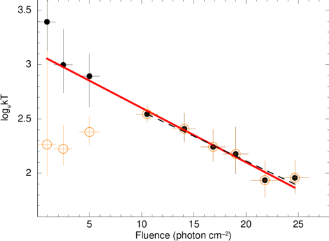
Figure 9: The evolution of temperature ($kT$) as a function of “running fluence” in single pulse GRB 080904 is shown — (i) $kT$ evolution of BBPL model fit (orange open circles), (ii) Higher BB temperature, $kT_{h}$ of 2BBPL fitted to the initial three bins, while BBPL fit is retained for the rest (filled circles). Both the evolution are fitted with a linear function (dotted line for the falling part of case (i), solid red line for case (ii)). The evolution match quite well at the overlapping region (see text for detail). Source: Basak & Rao (2012c)

10 The Lower BB In The XRT Window

It is clear from the above discussion that the lower BB can affect the spectrum in the initial bins giving a phenomenological break. As the lower BB temperature goes below the GBM/BAT sensitivity it is expected to be seen in the low energy detector, namely the Swift/XRT. This is a more direct proof of the evolution of the two BBs. However, this opportunity is very rare as the XRT observation starts with some delay. GRB 090618 is one of such cases where the XRT observation started during the late phase of the prompt emission. In Figure 10, we have shown the count rate lightcurve of the BAT and the XRT data. Note that the two observations overlap at the late prompt phase. The XRT observation starts at 125 s, where the falling part of the last pulse is still visible in the BAT energy band.

Figure 10: Lightcurve of GRB 090618. Count rate (arbitrary unit) is plotted as a function of time — BAT (black points), XRT (red points). Note the overlap of observation time of the two instruments. The XRT data is taken from $http://www.swift.ac.uk/xrt\_curves/$ (see Evans et al. 2007, 2009).

Table 5: Parameters of BBPL and 2BBPL model fit to the time-resolved data of GRB 090618 in 116.95-130.45 s

Interval	2BBPL							BBPL
	$kT_{h}$	$N_{h}$	$kT_{l}$	$N_{l}$	$\Gamma$	$N_{\Gamma}$	$\chi^{2}$	$kT$	$N$	$\Gamma$	$N_{\Gamma}$	$\chi^{2}$
$116.95-118.05$	$23.8_{-5.7}^{+7.1}$	$2.9_{-1.4}^{+1.3}$	$9.0_{-2.6}^{+2.5}$	$1.9_{-1.0}^{+1.0}$	$-2.4_{-0.3}^{+0.2}$	$541_{-215}^{+530}$	76.5 (102)	$14.8_{-1.8}^{+1.8}$	$1.7_{-0.5}^{+0.5}$	$-2.2_{-0.1}^{+0.1}$	$368_{-67}^{+90}$	79.8 (104)
$118.05-119.35$	$21.4_{-5.8}^{+5.6}$	$2.1_{-0.9}^{+1.2}$	$7.6_{-1.5}^{+1.3}$	$2.1_{-0.8}^{+0.9}$	$-2.3_{-0.2}^{+0.4}$	$304_{-137}^{+417}$	95.5 (102)	$10.2_{-1.1}^{+1.4}$	$1.4_{-0.3}^{+0.3}$	$-2.1_{-0.1}^{+0.1}$	$243_{-49}^{+58}$	100.6 (104)
$119.35-120.95$	$20.8_{-4.4}^{+4.4}$	$2.0_{-0.9}^{+0.9}$	$8.3_{-1.6}^{+1.7}$	$1.5_{-0.7}^{+0.8}$	$-2.4_{-0.2}^{+0.4}$	$412_{-163}^{+571}$	85.0 (102)	$12.6_{-1.4}^{+1.5}$	$1.4_{-0.3}^{+0.3}$	$-2.2_{-0.1}^{+0.1}$	$280_{-56}^{+73}$	88.7 (104)
$120.95-122.65$	$14.8_{-1.4}^{+1.9}$	$2.8_{-0.5}^{+0.6}$	$5.2_{-1.0}^{+1.8}$	$1.1_{-0.6}^{+0.7}$	$-2.4_{-0.2}^{+0.3}$	$276_{-163}^{+196}$	123.8 (102)	$13.4_{-0.8}^{+0.8}$	$2.1_{-0.3}^{+0.4}$	$-2.4_{-0.1}^{+0.1}$	$370_{-83}^{+120}$	127.5 (104)
$122.65-124.85$	$20.4_{-1.2}^{+1.5}$	$2.9_{-0.5}^{+0.3}$	$6.4_{-0.5}^{+0.5}$	$2.5_{-0.5}^{+0.6}$	$-3.6_{-0.8}^{+1.3}$	$4650$	105.1 (102)	$14.6_{-2.7}^{+2.4}$	$0.8_{-0.3}^{+0.3}$	$-2.3_{-0.1}^{+0.1}$	$338_{-74}^{+94}$	123.0 (104)
$124.85-127.25$	$24.1_{-10.1}^{+19.2}$	$1.0_{-0.6}^{+0.7}$	$8.7_{-3.8}^{+1.6}$	$1.3_{-0.9}^{+0.5}$	$-2.6_{-0.3}^{+0.4}$	$487_{-279}^{+687}$	91.3 (102)	$10.6_{-1.2}^{+1.4}$	$0.9_{-0.4}^{+0.4}$	$-2.3_{-0.1}^{+0.1}$	$276_{-88}^{+136}$	98.5 (104)
$127.25-130.45$	$15.3_{-3.4}^{+4.0}$	$1.0_{-0.4}^{+0.4}$	$5.2_{-0.9}^{+1.2}$	$1.2_{-0.4}^{+0.5}$	$-2.3_{-0.3}^{+0.4}$	$123_{-87}^{+226}$	91.5 (102)	$8.4_{-1.3}^{+1.7}$	$0.6_{-0.2}^{+0.2}$	$-2.3_{-0.1}^{+0.1}$	$189_{-45}^{+56}$	93.3 (104)

Notes: The bins are obtained by requiring $C_{\rm min}=1500$. Errors are $1\sigma$.

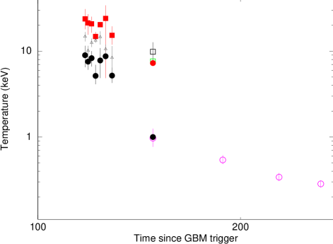
Figure 11: Evolution of BB temperature ($kT$) for different models are shown. The XRT data (open circles with magenta colour) is shown during 125-275 s post BAT trigger (last four points). The joint GBM-BAT data is fitted in the previous bins till 130.45 s post GBM trigger. Evolution of the following parameters are shown: (i) $kT$ of BBPL (grey open triangles), (ii) higher ($kT_{h}$) and lower ($kT_{l}$) BB temperature of 2BBPL model (red filled boxes, and black filled circles, respectively). Note that the evolution of $kT_{l}$ smoothly connects with the later evolution in the XRT. The data of the first XRT bin (125-165 s) is used for a joint BAT-XRT analysis. The corresponding $kT$ remarkably follows the two BB evolution of the previous bins (red filled circle for $kT_{h}$, and black filled circle for $kT_{l}$ in 125-165 s time bin; see text for detail).

Page et al. (2011) have studied this GRB, and have found an evidence of BB component in the XRT spectrum. They have used four time bins from 125-275 s, and one large bin in 275-2453 s. In all cases a BBPL model gives $>0.9999$ F-test significance as compared to a PL fitting. The x-ray spectral fits include absorptions due to galactic and intrinsic neutral hydrogen ($N_{\rm H}=5.8\times 10^{20}$ cm^-2, and $zN_{\rm H}=(1.82\pm 0.08)\times 10^{21}$ cm^-2). In Figure 11, we have shown the BB temperature in the XRT data by open circles with magenta colour (last four points). The time axis is shifted by 3.192 s, as there is a delay of BAT trigger from the GBM trigger by this amount of time. In order to find the connection of this BB with that in the higher energies, we study the time-resolved GBM and/or BAT spectrum in 116.95-130.45 s. The bins are obtained by requiring $C_{\rm min}=1500$ in the NaI detector having the highest count rate (n4). We have used both the GBM and the BAT for our analysis to constrain the parameters with good accuracy. In Table 5, we have shown the best-fit values of BBPL and 2BBPL model fit.

In Figure 11, we have marked the values of $kT$ as obtained by BBPL model fitting by grey triangles. The values of $kT_{h}$ (red filled boxes) and $kT_{l}$ (black filled circles) of 2BBPL model are also marked. Note that $kT$ of BBPL model in these initial bins will largely over-predict those in the later XRT data. Hence, these two BBs are not connected. In contrast, the lower BB temperature, $kT_{l}$ in the initial bins clearly shows the trend of later $kT$ evolution in the XRT data (compare the black filled circles in the initial 7 bins to the magenta open circles in the last 4 bins).

In order to find how the higher BB evolves, we fit the 125-165 s data of the BAT and the GBM data with a BBPL model. Note that if we get a BB temperature consistent with the evolution of $kT_{h}$ in this bin, then it shows that the lower BB must have gone below the GBM/BAT sensitivity level. We fit the data of this bin using BAT, joint BAT-GBM and joint BAT-XRT, all of which are found to be consistent with each other. The corresponding points are shown in Figure 11 by black open box, green open box, and red filled circle, respectively. Note that the BB temperature of this bin is clearly consistent with the trend of $kT_{h}$ evolution in the previous bins (compare with red filled boxes of the initial 7 bins). The corresponding lower BB temperature as found from the joint BAT-XRT analysis is shown by black filled circle in this time bin. The value of this lower BB temperature in this bin is consistent with that obtained by fitting a BBPL model in this bin (magenta open circle below the black symbol). To emphasize again, the GBM/BAT data and the XRT data of 125-165 s are fitted independently by using single BB models for either of them. It is quite remarkable that these two temperatures are fully consistent with the trends of $kT_{h}$ and $kT_{l}$, respectively, and also with the joint BAT-XRT data. Hence, the findings are consistent with the hypothesis that there are indeed two evolving BBs during the prompt emission phase.

Part III: A Simplistic Model

11 The Physical Model

1 List Of Observations:

Let us first list down the important features we have observed.

• (i) The prompt emission spectrum is not totally non-thermal. A Band only function either gives unphysical spectral index, or sometimes additional components are required. Most importantly, the additional parameters seem to show up for high flux case. Consider, e.g., GRB 090902B and GRB 100724B. The former can be fitted by a smoothly varying BB (multi-colour BB) along with a PL, while the later requires a separate BB component on top of a Band function. But, each of the spectra can be fitted with a 2BBPL model. We have also found that these GRBs are not special, all the bright GRBs with GeV photons, with single pulse, or multiple separable pulses are consistent with 2BBPL model. Though it is entirely possible that each GRB has a characteristic spectrum, but the fact that a single model can fit to all possible variety of GRBs strongly indicates a common radiation mechanism.

• (ii) We have also found that the two BBs of 2BBPL model are highly correlated. Both the temperature and normalization of these BBs have a ratio in the range $\sim 3-5$.

• (iii) The PL component of 2BBPL model is physically reasonable for synchrotron radiation. It is also found that the PL index becomes lower at the later phase. For example, GRB 081221 has the following evolution of indices in the rising and falling part of the constituent pulses — pulse 1: $-1.74_{-3.04}^{+\infty}$ to $-2.04_{-0.14}^{+0.28}$, pulse 2: $-1.94_{-0.11}^{+0.16}$ to $-2.15_{-0.08}^{+0.09}$. Hence, the spectrum becomes softer with time.

• (iv) GRBs with high GeV emission have a delayed onset of the PL component. This component becomes important at the later phase. On the other hand, GRBs with similar brightness in the GBM band, but an order of magnitude lower GeV emission have coupled PL and total flux evolution. The evolution of the PL in each case remarkably mimics that of the corresponding GeV emission.

2 A Spine-sheath Jet Model:

The model that we use to explain the observations listed above is a spine-sheath structure of the jet. This is one of the most attractive proposed jet structure based on both theoretical and observational requirement. On the theoretical side, a slowly moving sheath surrounding a fast inner spine is expected as the jet punctures through the envelop of the dying star. The material of the star forms a hot cocoon layer on the spine jet (Woosley et al. 1999, Mészáros & Rees 2001, Ramirez-Ruiz et al. 2002, Zhang et al. 2003, 2004b, Mizuta et al. 2006, Morsony et al. 2007). Even if the cocoon is absent, a MHD jet can have a collimated proton spine with wider neutron sheath (Vlahakis et al. 2003, Peng et al. 2005). On the observational ground a shaeth is invoked in a GRB jet to explain several observations, e.g., shallow decay phase of x-ray afterglow (Granot et al. 2006, Panaitescu et al. 2006, Jin et al. 2007, Panaitescu 2007), observation of jet break in radio as well as in optical and x-ray afterglow (Lipunov et al. 2001, Berger et al. 2003b, Sheth et al. 2003, Liang & Dai 2004, Huang et al. 2004, Wu et al. 2005, Holland et al. 2012). For example, Berger et al. (2003b) have studied the afterglow of GRB 030329 ($z=0.1685$) in the radio wavelength. They have found a jet break at 9.8 day, which together with the observed flux corresponds to a jet opening angle $\theta_{\rm sheath}\sim 17^{\circ}$. However, the optical and x-ray lightcurve also have an achromatic break at $\sim 0.55$ day corresponding to $\theta_{\rm spine}\sim 5^{\circ}$. The optical data also show a re-brightening corresponding to the peak of the second jet component. The ratio of collimation corrected energy of the two components is found to be $E_{\rm sheath}/E_{\rm spine}\sim 5$ i.e., a larger fraction of energy is carried by a much wider jet component. Recently, Holland et al. (2012) have studied the optical afterglow data of GRB 081029 ($z=3.8479$). The opening angle of the two components as required by the data is much smaller than GRB 030329 — $\theta_{\rm spine}\sim 0.86^{\circ}$, and $\theta_{\rm sheath}\sim 1.4^{\circ}$. In addition, unlike GRB 030329, the energetics of the two components are comparable to each other. It is not clear whether there are two classes of GRBs with completely different properties of the spine-sheath components.

Recently, Ito et al. (2013, I13 hereafter) have used a Monte Carlo simulation to study the emergent spectrum from a spine-sheath jet. They have considered the opening angle of spine and sheath as $0.5^{\circ}$ and $1^{\circ}$, respectively. They have injected thermal photons at a region of high optical depth and followed each photon till it escapes at the photosphere. With varying ratio of $\eta$ between the two components (in the range 1-4), and for different viewing angles ($0.25^{\circ}-0.75^{\circ}$), they have obtained some spectra which have the signature of the two BB components (Figure 5 of I13). The two thermal components are most prominent for a viewing angle near the spine sheath boundary. In addition to the BB components, I13 have found a PL with a high energy cut-off. The extra PL component is argued to be the extra hard component as seen for GRBs like 090902B.

3 Origin Of The Spectral Components

Let us consider the spine-sheath model of I13. We shall give some order of magnitude estimates as required by our observations. The assumptions are as follows. The coasting bulk Lorentz factor of spine and sheath regions are $\eta_{\rm sp}$ and $\eta_{\rm sh}$, respectively, and $\eta_{\rm sp}>\eta_{\rm sh}$. As $\eta=L/\dot{M}c^{2}$, the difference in its value in the two regions can occur due the difference in jet luminosity $L$, or mass flow rate $\dot{M}$. It is reasonable to assume that as the sheath should be baryon dominated, it has higher mass flow rate. The jet luminosity can be assumed equal.

A. Origin Of Two Blackbodies

The two BBs in this model appear from two photospheres of the spine and sheath. As the photospheric radius, $r_{\rm ph}\propto L\eta^{-3}$, we find that the photosphere of the spine ($r_{\rm ph,sp}$) occurs lower than that of the sheath ($r_{\rm ph,sh}$). Also, as the saturation radius, $r_{\rm s}\propto r_{\rm i}\eta$, where $r_{\rm i}$ is the initial injection radius, the saturation of spine occurs above the sheath ($r_{\rm s,sp}>r_{\rm s,sh}$). Now, we know that during the adiabatic expansion, the evolution of both bulk Lorentz factor ($\Gamma$) and co-moving temperature ($kT^{\prime}$) have a break at $r_{\rm s}$. The evolution of $\Gamma_{\rm sp}$ and $\Gamma_{\rm sh}$ are similar to each other ($\propto r/r_{\rm i}$) till $r_{\rm s,sh}$. After this radius the sheath stops accelerating and coasts with its corresponding value, $\eta_{\rm sh}$. The spine, however, accelerates till $r_{\rm s,sp}$ (note that $r_{\rm s,sp}>r_{\rm s,sh}$). The evolution of $kT^{\prime}$ can be written as follows (see I13).

$$kT^{\prime}\propto\left(\frac{L}{r_{\rm i}^{2}}\right)^{1/4}\times\left\{\begin{array}[]{ll}(r/r_{\rm i})^{-1}&\mbox{$r<r_{\rm s}$}\\ (r_{\rm s}/r_{\rm i})^{-1}(r/r_{\rm s})^{-2/3}&\mbox{$r>r_{\rm s}$}\end{array}\right.$$ (1)

Here $r$ is the radial distance from the centre of explosion in lab/observer frame. As an observer sees a boosted temperature from the photosphere, the temperature before the break is a constant and does not degrade due to the adiabatic cooling. However, after the saturation the observer temperature drops as $r^{-2/3}$, As the temperature degrades above $r_{\rm s}$, it is evident that the spine has a brighter and efficient photospheric emission than the sheath.

Now, if we consider that the phtosphere in both components occur above the saturation, then from equation 1, we get the observed temperature at $r_{\rm ph}$ as $kT\propto r_{\rm i}^{1/6}\eta^{8/3}L^{-5/12}$. The peak luminosity is found to be $L_{\rm p}\propto r_{\rm i}^{2/3}\eta^{8/3}L^{1/3}$. Note that both these quantities strongly depend on the coasting bulk Lorentz factor, $\eta$. Considering the same radius of initial energy injection ($r_{\rm i}$), and similar jet kinetic luminosity ($L$) for spine and sheath, the ratio of temperature and peak luminosity are $\propto\eta^{8/3}$. Note that the peak luminosity is a representation of the normalization of the two BBs in our analysis. Hence, from the above discussion, we need a ratio of $\eta\approx 1.5-1.8$, to get a ratio of temperature and normalization $\sim 3-5$. On the other hand, if we assume that the jet kinetic luminosities are not similar, then other ratios are possible. For example, I13 have assumed that $\dot{M}$ is the same for the two components, then the ratio of $L$ scales with $\eta$. Hence, we require a ratio $\eta\approx 1.6-2.0$ for temperature ratio of $3-5$. However, the corresponding normalizations have a ratio $4-8$. Note that the observation of Holland et al. (2012) indicates that the kinetic luminosity of the two components should be rather comparable. If the kinetic luminosity of the spine is lower than the sheath by a factor of $\sim 5$ (as required by Berger et al. 2003b), and the mass flow rate is lower by a factor of 10, then the ratio of $\eta$ is $\sim 2$. Hence, if the sheath is indeed the cocoon, the relative values of jet kinetic energy and mass flow rate ensures a moderate ratio of $\eta$, and hence, a reasonable temperature ratio $\sim 3-5$ is attained.

B. Origin Of The Power-law

As discussed, from the region above $r_{\rm s,sh}$, the sheath coasts with the value $\eta_{\rm sh}$, while the spine continues to accelerate. Hence a strong velocity shear occurs in the region $>r_{\rm s,sh}$. The photons crossing the spine-sheath boundary are Comptonized by electrons moving in the flow. Depending on the angle of incidence ($\theta_{\rm i}$) and scattering angle ($\theta_{\rm s}$), the photon either gains energy (up-scattered; $\theta_{\rm s}<\theta_{\rm i}$), or looses energy (down-scattered; $\theta_{\rm s}>\theta_{\rm i}$). I13 have shown that the average gain in up-scattering and in down-scattering are $\frac{1}{2}\left[1+\left(\frac{\Gamma_{\rm sp}}{\Gamma_{\rm sh}}\right)\right]$ and $\frac{1}{2}\left[1+\left(\frac{\Gamma_{\rm sh}}{\Gamma_{\rm sp}}\right)\right]$, respectively. Note that as $\Gamma_{\rm sp}>\Gamma_{\rm sh}$, the up-scattering denotes gain, while down-scattering denotes loss. The overall gain of this process is $>1$. As a result the synthetic photon spectrum is a power-law (see Figure 5 of I13). However, the acceleration is limited by the efficiency of Compton scattering. When the co-moving energy of the photon approaches the rest mass energy of electron, the Compton scattering approaches the Klein-Nishina regime, where the reaction cross section rapidly drops, leading to a very inefficient acceleration. I13 have obtained a sharp cut-off at $\sim 100$ MeV, which corresponds to a Lorentz factor ($\Gamma$) of $\sim 200$. Note that for higher $\Gamma$, the cut-off can occur at higher energy. In Figure 12, we have shown a schematic picture of a spine-sheath jet (the darker region shows the spine). We have marked the photospheres of the two components. Note that the spine photosphere is lower than that of the sheath. The prompt emission can occur in the photosphere and/or in the IS region with a delay. Photons crossing the spine-sheath boundary layer are Comptonized. Hence, these photons will also form a non-thermal component in the higher energy band.

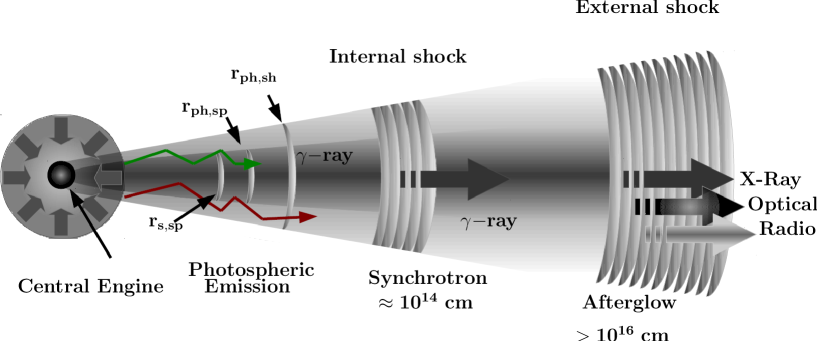
Figure 12: A schematic diagram of spine-sheath jet model. The spine efficiently emits thermal photon at the the photosphere ($r_{\rm ph,sp}$), while the sheath produces a second thermal component. The photons crossing the boundary layer (red and green zig-zag lines) are Inverse-Comptonized. The IS is delayed from these emissions.

4 Explanation Of The Observations:

Let us now use the spine-sheath structure of jet, and examine whether it is consistent with the observations we have shown.

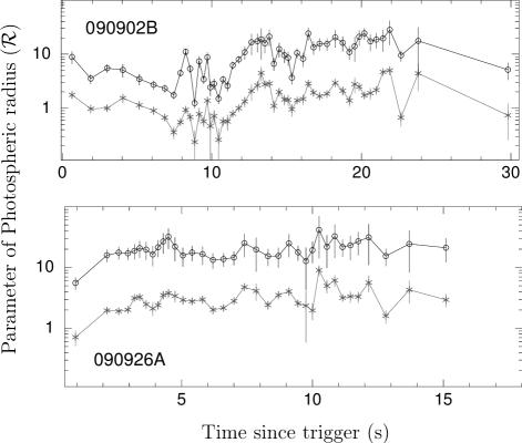
Figure 13: Evolution of the parameter $\cal{R}$ as a function of time for GRB 0909002B (upper panel) and GRB 090926A (lower panel). The actual photospheric temperature can be directly determined from $\cal{R}$. The symbols are: open circles (lower BB), and stars (higher BB). Note that higher BB has a lower $\cal{R}$, and the values are correlated throughout each burst. Source: Rao et al. (2014).

• (i) First note that the model naturally produces two BB spectra from the two photospheres. If we assume that both spine and sheath components have reached the saturation, then the final coasting value of their $\Gamma$ remains constant for the later part, with a ratio $\eta_{\rm sp}/\eta_{\rm sh}$. Now, the co-moving temperature ($kT^{\prime}$) of both spine and sheath undergoes adiabatic cooling. Hence, the later observed temperature ($kT\propto\Gamma kT^{\prime}$) should be correlated. Note that the sheath, having much lower $\eta$, has definitely reached the saturation before reaching the photosphere ($r_{\rm ph,sh}$). The spine, on the other hand, can reach $r_{\rm s,sp}$ after $r_{\rm ph,sp}$. In this case, the observed temperatures ($kT_{h}$ and $kT_{l}$) may not be correlated in the initial bins. Such cases can lead to diverse features in the temperature evolution before the break (as discussed in section 6.9).

• (ii) As discussed, the spine-sheath jet can effectively Inverse-Comptonize the photons crossing the boundary layer in the velocity shearing region. However, the emergent non-thermal component is found to be cut-off power-law (CPL) rather than a full power-law (PL). Hence, we shall probably need synchrotron (and /or IC) in the IS to account for a PL with no break in the observed GBM-LAT band. Note that the values of the PL index as found in our analysis remain within fast cooling regime of an optically thin synchrotron emission. Hence, the PL component can be a combination of both the processes.

• (iii) It is interesting to compare the location of photosphere of the two thermal components and check with the data. For this purpose, let us define the dimensionless quantity ${\cal{R}}$ (see Ryde & Pe’er 2009) as follows.

  $${\cal{R}}(t)=\left[\frac{F_{\rm Th}(t)}{\sigma T(t)^{4}}\right]^{1/2}$$ (2)

  Here $F_{\rm Th}(t)$ and $T(t)$ are respectively the flux and temperature of one of the BBs at a given observer time, $t$. As the physical photosphere is directly proportional to ${\cal{R}}$, an evolution of ${\cal{R}}$ shows the evolution of the actual photosphere. In Figure 13, we have shown the evolution of ${\cal{R}}$ (in units of $10^{-19}$) as a function of time for two GRBs, namely GRB 090902B (upper panel), and GRB 090926A (lower panel). Ryde & Pe’er (2009) have calculated ${\cal{R}}$ for a sample of bursts, and have shown that the quantity either increases or remains constant throughout the prompt emission. The later behaviour is found in these two GRBs — the photospheres of both the BBs remain steady throughout the bursts (see Figure 13). Note that the value of ${\cal{R}}$ for higher BB (stars) is always lower than that of the lower BB (open circles), and the values are correlated.

  Let us calculate the ratio of the photospheric radius based on the ratio of temperature and normalization.

  $$\frac{\cal{R}_{\rm spine}}{\cal{R}_{\rm sheath}}=\left(\frac{N_{\rm spine}}{N_{\rm sheath}}.\frac{T_{\rm sheath}^{4}}{T_{\rm spine}^{4}}\right)$$ (3)

  With a ratio of 3 for both the temperature and normalization, we get $\cal{R}_{\rm spine}\approx$ 0.2$\cal{R}_{\rm sheath}$. This result is consistent with the spine-sheath jet model for a ratio of $\eta\sim 1.5$, and assuming similar kinetic luminosity of both the components.

• (iv) Note that compared to the radius of IS region, the photospheric radius ($r_{\rm ph}$) of the two components are of the same order. Hence, the BB spectrum are nearly simultaneous. In our analysis we have found that the normalization (and flux) of the two BBs are highly correlated. Also note that the IC of photons within $r_{\rm ph}$ will be simultaneously detected with these two BBs. Hence, all these events are nearly simultaneous. As discussed, the non-thermal component of this emergent spectrum is a PL with a cut-off near 100 MeV. Hence, the GRBs with these three components will have less GeV emission. In our analysis, we have indeed found such GRBs (see Figure 6 — case C and D). Note that these two GRBs, despite having high GBM count, have very little LAT emission. Also note from this figure that the non-thermal component of both these GRBs have coupled total and PL evolution. Hence, the spectra of these GRBs are probably composed of three components — two BBs and a PL with a much steeper slope in the GeV range. All these components are nearly simultaneous as supported by the spine-sheath model as well as our observation.

• (v) The radius where the ISs are formed is at least three order of magnitude higher than the photospheric radius. Hence, the IS will be delayed. As the PL of 2BBPL model is always consistent with the fast cooling synchrotron spectrum, this emission is possibly dominant in generating the PL of 2BBPL model. As this spectrum extends to GeV energies, the GRBs accompanying efficient IS will produce GeV emission. Note that the PL component, in this case, will be delayed from the thermal emission. Hence, the model is consistent with our finding that GRBs with delayed PL emission are LAT bright. Note that we expect both synchrotron and IC in the IS regions, and the corresponding spectrum can be approximated as PL. However, for GRB 0909002B, we have shown that the required circumburst density is too high to accommodate SSC as a dominant component. Note that for this GRB we have found that the spectral slope in the keV-MeV data is fully consistent with that in the GeV data. Hence, the synchrotron spectrum does not have a break in the observed band. However, for GRB 090926A, there is a break at a very high energy.

12 Discussion

In this final chapter, we have proposed a simplistic model to explain the observations of prompt emission spectrum in conjunction with the observation of GeV and x-ray data. We would like to point out that though the existence of the 2BBPL model has strong observational supports, the physical model which we have suggested may not be unique. Perhaps the model may be a simplification of a more complex and fundamental phenomenon. A modification of the simplistic model, or a completely different physical process is not ruled out. For example, consider the Cannonball model (Dado et al. 2002, Dar & de Rújula 2004, Dado et al. 2007). In this scenario, the central engine releases the ejecta in a sequence of ordinary matter (“cannon-balls”). The energy is released via particle-particle interaction rather than shock generation or photospheric emission. In this model, the cannon-balls can give rise to blue-shifted bremsstraulung and IC of the ambient photons. If the two BBs found in our prompt emission study are related to the coexisting glories of two photon fields, then the higher BB temperature can be identified with a typical photon bath in the pre-supernova region (for $\Gamma\sim 100$, a few eV photon is boosted by a $\Gamma^{2}$ factor, producing $\sim 100$ keV), while the lower BB can be produced by some other mechanism like bremsstrahlung. Note that as the same cannonball produces both these emissions, the temperatures should be correlated. Such a very different model, in principle, can conform with our observation. Even in the context of the standard fireball model, the IS can produce an effective pair photosphere. Then the thermal emission is likely to be Comptonized BB emission from the photosphere. A variety of such complications over the simple two-component model can be conceived.

The origin of the two components of GRB jet is also an open question. In the cocoon model of sheath, the opening angle is about three times larger than the spine, while the coasting Lorentz factor ($\eta$) of the spine is about five times higher. In our analysis, we require a much lower ratio of $\eta$. It is important to note that as the observations indicate $L_{\rm sh}>L_{\rm sp}$ (Berger et al. 2003b), and we expect $\dot{M_{\rm sh}}>\dot{M_{\rm sp}}$, it is rather possible that the ratio of $\eta_{\rm sp}/\eta_{\rm sh}$ ($\eta\sim L/\dot{M}$) is moderate, and not too high. This is consistent with our finding. The observation of the prompt emission does not put any constraint on the opening angle. Hence, the afterglow observation can give further clue on the origin of the structured jet. Note that observation of Berger et al. (2003b) and Holland et al. (2012) require very different jet structure both in terms of energetics and opening angle. A much wider sheath (Berger et al. 2003b) is probably an indication of the cocoon structure.

We would like to mention that the spine-sheath boundary is not necessarily as sharp as it is assumed in the simplistic model. There can be smooth roll-over between the two regions. A full roll-over (Gaussian jet, Zhang et al. 2004a) will indeed produce a multicolour BB. Recently, Lundman et al. (2014) have considered a jet with a uniform spine, but a graded sheath i.e., the Lorentz factor of the sheath falls off gradually as a PL function of the angle from the jet axis (Spine: uniform $\Gamma_{0}$, sheath: $\Gamma(\theta)\propto\theta^{-p}$). They have studied the polarization properties in such a structured jet, and have found that for a narrow jet ($\theta_{j}\sim 1/\Gamma_{0}$) and steep gradient ($p\gtrsim 4$), the polarization can reach $\sim 40\%$. In recent years, high degree of polarization are indeed reported in a few cases (Yonetoku et al. 2012, Toma et al. 2012, Götz et al. 2013, Mundell et al. 2013, Wiersema et al. 2014). The polarization measurement in the optical afterglow (e.g., Wiersema et al. 2014) is argued to be a definite signature of synchrotron emission. However, as discussed, the finding of polarization in the prompt emission phase (e.g., Götz et al. 2013) is not necessarily associated with a synchrotron radiation. Lundman et al. (2014) have also shown that the spectrum below the thermal peak appears as a non-thermal spectrum due to aberration of light. The higher energy part produces a cut-off PL due to the similar mechanism as considered by I13.

Chapter 7 Summary and Future Directions

1 The First Phase Of The Final Stage

A gamma-ray burst (GRB) appears as an intense flash in the otherwise dark $\gamma$-ray sky. While one class of GRBs mark the cataclysmic event at the final evolutionary stage of a massive star (long GRBs), the other class, namely the short GRBs are probably the outcome of NS-NS, or NS-BH mergers. Our knowledge about the progenitors of these two classes is based on the environment of their formation, and other observational evidences. Despite the differences in the progenitor and environment, the mechanism of the prompt emission and the subsequent afterglow is similar for the two classes of GRBs. It is quite fortuitous that the first phase of a GRB is so luminous in none other than the $\gamma$-ray band so that the open $\gamma$-ray detectors can detect the events occurring at random directions from the edge of the universe. For example, compare a GRB with a supernova, which is bright in the optical wavelengths, and is detected by continuous scanning of the sky in this band. Due to the absorption of optical light a supernova cannot be observed farther than redshift, $z\sim 1.7$, with the majority found at much lower redshifts. In comparison GRBs can be observed at high redshift (the highest two are $z=9.4$, and $z=8.2$).

This thesis is primarily aimed at understanding the prompt emission phase of the long GRB class. In spite of the phenomenal discovery of the cosmological distance, and understanding a great deal of the environment, classes, and the afterglow phase, the emission mechanism of the very first phase of a GRB is still a matter of intense debate. It is important to understand the prompt emission phase in order to understand the progenitor, central engine, and the jet launching mechanism. In the absence of a detectable gravitational wave, the prompt emission characteristics seem to be the only direct signature of the central object. In addition, prompt emission provides the initial condition for the subsequent afterglow emissions, and is directly connected with the x-ray and GeV emission. Through extensive study of the prompt emission data provided by Swift and Fermi satellite, we have obtained several interesting results, and have found strong indication of such connections. In this final chapter, we shall summarize the results of our analysis, our understanding of the GRB phenomenology in general, and the possible future extension of our study.

2 Summary and Conclusions

Let us first summarize the main conclusions discussed in the thesis.

1 Simultaneous Timing And Spectral Description

We have attempted to combine the timing description, $F(t)$, and the spectral description, $F(E)$ to describe GRBs simultaneously in time and energy domain, $F(t,E)$. Such description is solely motivated by the need for using the full information of the data to capture rapid spectral evolution during the prompt emission phase. The constituent broad pulses of a GRB are chosen for this purpose as the spectral evolution is a pulse property, rather than a burst characteristic. We have used GRB 090618, one of the brightest GRBs in the Fermi era, and having four broad pulses with a precursor. We assume that the lightcurve of each pulse can be described by an empirical model with exponential rise and decay part (Norris et al. 2005) — $F(t)=A_{\rm n}f_{\rm n}(t,\tau_{1},\tau_{2},t_{\rm s})$. The instantaneous spectrum is assumed as a Band function (Band et al. 1993) — $F(E)=A_{\rm b}f_{\rm b}(E,\alpha,\beta,E_{\rm peak})$. In addition, the evolution of $E_{\rm peak}$ is assumed to have a hard-to-soft evolution (Liang & Kargatis 1996) — $E_{\rm peak}=f_{\rm LK}(\phi(t),E_{\rm peak,0},\phi_{0})$, where, $\phi(t)$ is the time integrated flux from start of the pulse to time $t$, called “running fluence”. This quantity relates the spectral and timing properties and leads to the simultaneous description. We have developed a XSPEC table model for each pulse to determine the model parameters — initial peak energy ($E_{\rm peak,0}$), and characteristic evolution parameter ($\phi_{0}$).

The best-fit model parameters are used to reconstruct each pulse. These are shifted and added to generate a 3-dimensional model (flux as a function of time and energy) of the entire burst. Such a 3D description has immense flexibility as the derived timing and spectral parameters can be derived and checked against the data. In particular,

• (i) we construct the lightcurve of the GRB in various energy bands, and find remarkable similarity of the data with the synthetic lightcurves.

• (ii) We derive the width variation of each pulse with energy, and find agreement with the data. It is expected that the width should increase with decreasing energy. The first two pulses indeed show such width variation. However, the data of the last two pulses indicate an “anomalous” width broadening in the lower end of the GBM energy band. This phenomenon is also shown by our pulse model. It is quite remarkable that such a minute detail of pulse characteristic is adequately captured, and explained as due to some particular combination of a few model parameters.

• (iii) We also deduce the delay of the high energy bands with respect to the lowest energy band for each pulse. We always find a soft delay, which is a direct consequence of the assumption of hard-to-soft spectral evolution. The spectral lag as calculated by our model also conforms with that calculated using the data directly.

The fact that all the derived parameters agree with those obtained by using the data directly confirms that the pulse description is correct. In addition, we get a better handle on the data as the timing and spectral description can be simultaneously obtained with any desired resolution. The limitation of our model is that the functions used to achieve it are all empirical. In spite of this limitation, the fact that the model correctly predicts the pulse characteristics, possibly indicates a fundamental process responsible for a broad pulse generation. We would like to emphasize again that the pulse description is quite generic. Any spectral and timing model, whether empirical or motivated by theory, can be connected by means of a description of the spectral evolution.

2 Improved GRB Correlation

The crucial step for analyzing the prompt emission data is the realization of the broad pulse structure in the lightcurve. The rapid variability on the broad pulses are considered to be independent. As we have shown that a full burst can be re-generated by adding the individual broad pulses, it is interesting to study each pulse separately. In particular, we have studied GRB correlations in the individual pulses. For this purpose, we have collected a sample of GRBs with secure redshift measurement, and have used the pulses for Amati correlation (Amati et al. 2002, $E_{\rm peak}-E_{\gamma,\rm iso}$). We have found that the pulse-wise Amati correlation is significantly better (Pearson correlation, $r=0.89$, $P_{\rm r=}2.95\times 10^{-8}$, Spearman rank correlation, $\rho=0.88$, $P_{\rho}=4.57\times 10^{-8}$) than both the time-integrated ($r=0.80$, $P_{\rm r=}9.6\times 10^{-3}$, $\rho=0.75$, $P_{\rho}=2.0\times 10^{-1}$), and time-resolved correlation which is not accounted for the broad pulses ($r=0.37$, $P_{\rm r=}9.5\times 10^{-3}$, $\rho=0.45$, $P_{\rho}=3.0\times 10^{-4}$).

As we have developed a simultaneous pulse model, it is interesting to use this model to see the improvement in the GRB correlation. The $E_{\rm peak}$ used in the pulse-wise correlation is a pulse-averaged quantity, and consequently the information of spectral evolution is lost. Hence, it is important to replace $E_{\rm peak}$ by $E_{\rm peak,0}$ which is a constant characterizing the peak energy at the beginning of a pulse. We have found that a pulse-wise $E_{\rm peak,0}-E_{\gamma,\rm iso}$ correlation is better considering the Pearson correlation ($r=0.96$, $P_{\rm r=}1.6\times 10^{-12}$). However, the Spearman rank correlation, which is a robust estimator of the correlation (Macklin 1982), is similar ($\rho=0.87$, $P_{\rho}=1.43\times 10^{-7}$). The intrinsic data scatter ($\sigma_{\rm int}$) per data points are also similar. In addition, we have found in later analysis that the HTS spectral evolution is not universal. Hence, in a later study, we have used the pulse-wise Amati correlation using $E_{\rm peak}$ instead of $E_{\rm peak,0}$ for a larger set of GRBs (19 GRBs with 41 pulses). We have found a reasonable correlation ($r=0.86,P_{\rm r}=1.50\times 10^{-13};\rho=0.86,P_{\rho}=7.47\times 10^{-14}$). We have studied the possible redshift evolution of the correlation parameters, and have found it insignificant (within $\triangle\chi^{2}=1.0$). To find possible bias due to the hardness at the beginning of a GRB, we have studied the correlation in the first/single pulses and the rest of the pulses. We again find no statistically significant difference. Improvement of GRB correlation within the constituent pulses is a significant step in understanding the pulse emission mechanism. It possibly indicates that the pulses are independent episodes of the prompt emission. In addition, the pulse-wise correlation signifies that the Amati-type correlations are real and devoid of selection effects. However, due to large intrinsic scatter even such a tight correlation is still far from being usable as cosmological luminosity indicators (Arabsalmani et al., in preparation). In future, if a pule-wise correlation with an order of magnitude lower intrinsic scatter is indeed available, it can give a good constraint on the inferred redshift of a GRB, and the cosmological parameters due to the application of different pulses of the same GRB.

3 Alternative Models Applied To GRBs With Single Pulses

The 3D pulse model is developed with the assumption that the instantaneous spectrum is a Band function. Though the Band function is statistically the most appropriate standalone model of the prompt emission spectrum, it is a completely phenomenological model. In the internal shock model of a GRB, the shocks are produced at a larger radius from the photosphere. The electrons accelerated by Fermi process in the shock gyrate around the aligned magnetic field (also developed by the shock) to produce synchrotron emission. Hence, it is natural to expect that the emergent spectrum should follow the synchrotron predictions. It is shown that the value of the low energy index ($\alpha$) of the Band function often crosses the limit due to synchrotron radiation. As we expect the electrons to cool fast during the prompt emission phase, the predicted index should be softer than -3/2, i.e., $\alpha>-3/2$ is forbidden (the so called “fast cooling line of death”). Even for slow cooling, the index should be less than -2/3 (“slow cooling line of death”). However, the spectral slope are often higher than both these values (Preece et al. 1998, Crider et al. 1999, Kaneko et al. 2006).

Our inability to associate Band function with a physical model instigates the search for alternative models. We have used three alternative models for our purpose : (i) blackbody with a power-law (BBPL), (ii) multi-colour blackbody with a power-law (mBBPL), and (iii) two BBs with a PL (2BBPL). Note that all the alternative models segregate the spectrum into a thermal and a non-thermal part. The thermal part is either as narrow as a Planck spectrum (BB), or have a surface profile (mBB), or have two BBs. We have applied these models on high flux GRBs with single pulses. Such a set is chosen in the hope of understanding a single pulse, and then use the knowledge for a complex GRB with multiple pulses.

• (i) We have found, based on $\chi^{2}$ values, that all the models are better than the BBPL model, though we could not find which among the other three is the best. Based on the value of $\alpha$ we have found that the Band function does not conform with a synchrotron interpretation. On the other hand, the PL index of the BBPL model ($\Gamma$) is lower than -3/2. As $\Gamma$ of mBBPL and 2BBPL are always found lower than that of BBPL, the corresponding values of $\Gamma$ are well within the fast cooling regime of synchrotron radiation. Based on our analysis, we suggest that either mBBPL or 2BBPL is the preferred model for the prompt emission spectral data. It is interesting to find that the two BBs of 2BBPL model are highly correlated in terms of their temperature and normalization. Hence, if the 2BBPL model is the correct spectral model, the origin of the two BBs should be connected.

• (ii) We have also studied the evolution of $E_{\rm peak}$ and $kT$ with time, and have identified two classes of GRBs — hard-to-soft (HTS) and intensity tracking (IT). As some of the GRBs with single pulse are indeed IT, such a spectral evolution must be physical (at least in some cases) rather than a superposition effect due to the preceding pulse.

• (iii) Important differences are found between the two classes e.g., HTS have generally higher values of $\alpha$ than the IT GRBs. We have also found that the PL component of three HTS bursts have delayed onset than the thermal component, and this component lingers at the final phase of the prompt emission. Interestingly, all these GRBs have reported GeV emission in the Fermi/LAT observation.

4 Parametrized Joint Fit: The 2BBPL Model

Based on the $\chi^{2}$ values and physical arguments, we have seen that the most preferred models of the prompt spectral data are mBBPL and 2BBPL, rather than the Band or BBPL model. Application of various models on GRBs with single pulse is the first step towards understanding the emission mechanism. Though single pulses are ideal for analysis purpose, majority of GRBs have either clean multiple pulses or largely overlapping pulse structure. It is not clear whether the difference between these classes are due to the difference in fundamental radiation process or the difference of the number of episodes.

In order to find the correct model, we have developed a new technique of spectral analysis, namely “Parametrized Joint Fit”. The main motivation of this technique is to reduce the number of parameters in the time-resolved spectroscopy by parameterizing and tying model parameters over certain time interval. We note e.g., the evolution of $kT$ of BBPL model can be parameterized as $kT\propto t^{\mu}$, and the PL index ($\Gamma$) can be tied separately in the rising and the falling part of a pulse. Such parametrization and tying scheme is applied for all models to achieve similar number of free parameters for all of them. For our analysis, we have chosen 2 bright GRBs with clean multiple pulses and 3 bright GRBs with highly variable lightcurves. For the latter class, we have dropped the parametrization scheme.

The results of our analysis is summarized as follows.

• (i) The data agrees with mBBPL and/or BBPL model with similar or better $\chi^{2}$ than the Band function at the rising part. Also, the value of $\alpha$ of Band function is higher than -2/3, which disfavours a synchrotron origin. The PL index of the alternative models are within fast cooling regime of synchrotron. Hence, the rising part of each pulse has both a thermal and a non-thermal component. In the falling part, however, the Band function is preferred in terms of $\chi^{2}$, and the value of $\alpha$ is less than -2/3. The PL index of the other models also lower than that in the rising part. Hence, the spectrum has a definite transition from a thermal to synchrotron domination.

• (ii) As there is a definite transition of the spectrum, and the second pulse repeats the similar behaviour, it can be inferred that the pulses are independent, and possibly represent two episodes of the central engine activity.

• (iii) A comparison with 2BBPL model with all other model shows that this model is either better or comparable to mBBPL and Band function. 2BBPL model, being an extension of the BBPL model shows high significance of adding the extra BB. More importantly, while the $F$-test significance level of the other models (mBBPL, Band) in comparison with BBPL model decreases with finer bin size (e.g., significance of mBBPL/BBPL changes from $2.55\sigma$ to $1.56\sigma$ in the rising part of pulse 2), the significance of 2BBPL over BBPL model remains similar ($9.29\sigma$ to $9.66\sigma$). This signifies that the second BB is required to capture the spectral evolution. The PL index of 2BBPL model has similar characteristic as the BBPL and mBBPL models.

• (iv) For bright GRBs with highly variable lightcurve, we obtain similar conclusions. The time-resolved spectra of GRB 090902B shows a definite improvement in the residual while fitted with a 2BBPL model as compared to the Band and BBPL models. The mBBPL model gives a similar fit statistics as the 2BBPL model.

5 Consequences and Predictions of the 2BBPL Model

In the final chapter, we have discussed about various consequences and predictions of the 2BBPL model. The fact that the spectral analysis of the prompt keV-MeV data has predictive powers for both lower and higher energy data, gives us the confidence that the spectral model is correct. In the following we list the consequences and predictions.

• (i) The evolution of the two BBs (with or without a break) can lead to an increasing temperature during the early part of a pulse. In the standard fireball model the temperature can have a break due to the transition from an accelerated to a coasting phase, and provided that the photosphere occurs below this transition radius. The evolution below the break is expected to be constant (for radiation dominated fireball), or decreasing (for magnetic field dominated fireball). An increasing temperature is unexplained. It is possible that an averaging of the temperature of two BBs, both having characteristic evolution, give rise to such a phenomenological evolution. In the later part, the lower BB may go below the bandwidth of the GBM/BAT, showing no effect on the evolution. We have illustrated such a hypothetical situation with a single pulse GRB.

• (ii) If the lower BB indeed goes below the bandwidth of the higher energy detectors, it should become visible in the low energy detector like the Swift/XRT, provided the data is available in the late prompt emission phase. At a much later time, the emission may be afterglow dominated. Hence, it is important to obtain the XRT data as early as possible. For GRB 090618, we have found that the XRT data in WT mode is available from 125 s after the trigger. During this time the falling part of the last pulse is still visible in the GBM/BAT band. The GBM/BAT data in the falling part of the pulse fitted with a BBPL model gives a much higher trend of temperature evolution compared to that found in the XRT data. However, the lower BB of the 2BBPL model fitted to the same data shows a impressive similarity. In addition, a BBPL model fitted to the GBM/BAT data of the first XRT bin falls perfectly on the predicted evolution of the higher BB of 2BBPL model. Such a finding confirms the presence of a separate BB component in the prompt emission spectrum.

• (iii) In addition to the data in the lower energy band, we find a remarkable prediction for the very high energy band covered by the Fermi/LAT. First we investigate the basic difference of the prompt keV-MeV spectrum of GRBs with similar GBM brightness, but an order of magnitude difference in LAT brightness. We fit the spectral data obtained only from the GBM with a 2BBPL model, and try to predict which among these classes should lead to high GeV emission. We find that the LAT-bright GRBs have a delayed onset of the PL, and this component becomes progressively important at a later phase. GRBs with similar GBM count, but having lower LAT count do not show such a behaviour. In other words, GRBs which show a delayed and lingering non-thermal component in the prompt emission should accompany high GeV emission. The current strategy of re-pointing Fermi to observe GeV emission is to target the GBM-bright GRBs. We propose that the re-pointing criteria should include moderately bright bursts with delayed PL component. Such an inclusive strategy may increase the LAT sample size.

• (iv) One of the puzzles in the comparative study of GeV emission and keV-MeV emission is the poor correlation between these components. It is not clear why GRBs with similar GBM brightness produce seemingly different GeV photons. As the PL component of the 2BBPL model shows a similar evolution as the GeV emission, we study a correlation between the fluence of the PL component with that of the GeV component. We find that the correlation is strong (Spearman rank correlation coefficient, $\rho=0.81$, $P_{\rho}=9.23\times 10^{-5}$), and it is unaffected by the presence of another variable, namely total GBM fluence ($D=2.3$).

6 Physical Origin: A Spine-sheath Jet

Based on the observations, 2BBPL model seems to be the most preferred model for the prompt emission spectrum. We propose a spine-sheath jet structure as a simplistic physical model to explain the observations. Let us summarize the major points.

• (i) The two BBs are natural consequence of the spine-sheath jet. If the coasting bulk Lorentz factor of the spine and sheath are $\eta_{\rm sp}$ and $\eta_{\rm sh}$ respectively, then the observed temperature and normalization above the saturation radius will always show a ratio $(\eta_{\rm sp}/\eta_{\rm sh})^{8/3}$. As $\eta\equiv L/\dot{M}c^{2}$, and we generally expect the spine to have higher $\dot{M}$, the sheath will show higher temperature and normalization. Also, note that the jet luminosity ($L$) as found by observation of the two components are either comparable, or sheath has a higher value. Hence, we do not expect a large ratio of $\eta$. For a nominal ratio of temperature and normalization as found in our observation, we require the ratio of $\eta=1.5-2.0$.

• (ii) In the velocity shear region, the jet structure Comptonize the photons crossing the boundary layer. As the photons on an average gain in energy, the emergent spectrum is a PL. This spectrum also has a cut-off due to decreasing cross-section at very high energy $\sim 100$ MeV. Hence, it is likely that some GRBs should have a cut-off PL (CPL) as the non-thermal component. However, GRBs with PL at very high energies (GeV) require other processes. As these processes are delayed, the GeV emission should also be delayed. This supports the observation that GRBs with delayed PL component have high GeV emission.

• (iii) Using the data of two GRBs, and with an order of magnitude calculation, we have also shown that the photosphere of the spine should occur at a lower radius than the sheath, which is also required by the model.

3 Future Directions

1 Analyzing The GBM Data To Predict The LAT Data

One of the remarkable results of our analysis is finding a connection between the GeV and keV-MeV emission. The fact that the delayed onset of the PL component indicates high GeV emission can be used for targeting this category of GRBs for the LAT observation. For off-axis GRBs from the LAT field of view, this strategy can increase the sample size of GRBs with LAT detection, and can shed light on the ongoing research in identifying potential GRBs with high energy emission. Such data needs to be quickly handled, and the analysis results should be immediately available. As our analysis is dependent only on the lower energy spectrum, only the GBM data is targeted. From 2012 November 26, the GBM is supplying continuous time-tagged event data (TTE) with $2\mu$s resolution. The data are sent through TDRSS message within a few seconds to the GBM’s Instrument Operation Center (GIOC). The GBM software is implemented to analyze the characteristics of the event, classify the object, and provide a crude event location. If a GRB is detected, the sky location is sent to the LAT. If the LAT monitoring reveals an increasing $\gamma$-ray flux, it sends an autonomous re-point recommendation (ARR) to the spacecraft. Generally the spacecraft accepts this request and performs a slew to the sky location of the target. An observation of a GRB by the LAT is performed for the next 2.5 hour including earth occultation.

In order to implement our finding for the LAT observation, we require science data of the GBM rather than the preliminary flux and localization data. For the data analysis, an automatized software should be developed. This software should analyze the GBM data in nearly real time, and it should report any signature of delayed PL component in the prompt emission data. For moderately bright GRBs, such an analysis can indicate a high GeV emission, which otherwise might have been missed based only on the flux level. Note that such a procedure crucially depends on the quickness of receiving the GBM science data which in practice can take several hours. Even if the procedure may not be used in the current strategy used by the Fermi satellite, it may prove useful to get an insight on the radiation process nonetheless, and may be used for later missions.

2 Physical Model Of The Prompt Emission

Through extensive data analysis, we have shown that the preferred model of the prompt emission is a 2BBPL model. Though this model is applicable for all variety of GRBs, it is important to establish a physical model for such a functional form. We have suggested a tentative physical picture within the frame work of the standard fireball model, namely a spine-sheath jet structure. We have shown that a fast moving spine with a slow sheath layer can indeed give rise to two BB components. It also produces a PL component by inverse Comptonizing the photons crossing the spine-sheath boundary. However, it is clear that shocks outside the photosphere are also required to explain a PL with no break in the LAT energy band. Both the mechanisms, in principle, can operate for the production of the non-thermal spectral component.

It is important to find out the relative contribution of the two components in order to constraint the physical parameters e.g., Lorentz factor, energy in the magnetic field etc. In this context, it is useful to employ physical function of synchrotron model (see e.g., Burgess et al. 2011). Such functions require electron distribution, Lorentz factor, magnetic field etc. Hence, the fitting directly gives these quantities. Various components in addition to the simple synchrotron model can be easily conceived, e.g., one can implement inverse Compoton (IC) in the internal shock to account for the high energy component. Using such models can give further insight in the production of the non-thermal component of the spectrum. However, these models are computationally expensive. As we are more interested in studying spectral evolution, the models should be made fast to be usable for time-resolved spectroscopy with parameterized-joint fitting.

3 Afterglow Observations

In this thesis, we have primarily discussed about the prompt emission phase. It is important to connect the inferences of the prompt emission to those of the afterglow. Though the afterglow emission is mostly related to the circumburst environment, the prompt emission sets the initial conditions in terms of total energy, energy in the thermal and non-thermal component and energy in the two components of the jet. Hence, a full prompt-afterglow analysis can constraint these quantities and establish the connection. For example, an early indication of delayed PL emission indicates GeV emission. Hence, it is interesting to perform afterglow observation in other wavelengths for this class of GRBs. As a two-component jet model naturally explains the observations during the prompt emission, it is important to establish this model on the basis of afterglow observations.

A two component jet has interesting observational signature e.g., re-brightening of the optical flux and double jet break in the x-ray/optical and radio (e.g., Berger et al. 2003a, Holland et al. 2012). Such signatures may give important constraints on the jet opening angle and the correct energetics of each component. While we obtain the $\gamma$-ray energy from the observation of prompt emission, the correct jet kinetic energy can be obtained by afterglow data and the observed jet break. It is worthwhile to point out again that the opening angle and jet kinetic energy obtained for two GRBs can be very different For example, Berger et al. (2003a) have found opening angles: $\theta_{\rm spine}\sim 5^{\circ}$, $\theta_{\rm sheath}\sim 17^{\circ}$, and $E_{\rm sheath}/E_{\rm spine}\sim 5$. Holland et al. (2012), on the other hand, have found $\theta_{\rm spine}\sim 0.86^{\circ}$, $\theta_{\rm sheath}\sim 1.4^{\circ}$, and $E_{\rm sheath}/E_{\rm spine}\sim 1$. Observations of a variety of such GRBs might provide important clues on the energy budget of each component, and the jet launching mechanism in general.

It is interesting to note that jet-breaks are relatively rare in Swift era ($\sim 12\%$; Liang et al. 2008, Racusin et al. 2009). Such observations even challenge the consensus of a GRB jet. Alternatively, the unobserved jet-break may be attributed to the uncertainties and bias in the observations (e.g., Curran et al. 2008, Kocevski & Butler 2008, Racusin et al. 2009), and/or smoother break due to off-axis viewing angle (e.g., van Eerten et al. 2010). Recently, Zhang et al. (2014) have investigated whether a jet-break is indeed present at a much later time and at a much deeper level of sensitivity than the Swift/XRT ($10^{-14}$ erg cm^-2 s^-1). They have used Chandra/Advanced CCD Imaging Spectrometer (ACIS) for a set of 27 GRBs, and have found 56% of jet-break. They have also performed a Monte Carlo simulation to show that the off-axis effects are indeed important to interpret a jet-break. It is interesting to investigate how the interpretations of an observed jet-break change with two components in the jet. For example, the proposed break will be affected by the presence of a much wider sheath component.

4 Clues From Other Objects

Additional information of the spectral model and jet structure can be obtained by comparing the observations of GRBs with other astrophysical objects. Though each of the objects would show a characteristic property, the underlying jet launching mechanism and radiation process should provide important clue on whether the processes are similar, diverse or follows a continuity. In the following, we have listed some of the objects which might prove very useful in studying these properties in a general sense.

I. X-ray Flashes (XRFs)

XRFs are lower energy cousins of GRBs and are believed to be a subset of the LGRB class, due to the similarity of LC, spectrum and the SN association in a few cases (Soderberg et al. 2005). XRFs were extensively studied with High Energy Transient Explorer 2 (HETE-2) (Heise et al. 2001, Kippen et al. 2003). The peak energy ($E_{\rm peak}$) and hardness of XRFs are found to be lower than the typical GRBs. Liang & Dai (2004) using a combined sample of GRB and XRF have found a tentative bi-modality in the $E_{\rm peak}$ distribution, which has peaks at $\lesssim 30$ keV and $\sim 160-250$ keV. Various intrinsic and extrinsic models are suggested to explain the mechanism of XRFs (see Zhang 2007b for a detailed discussion). Various speculations in the intrinsic differences are (i) XRFs are fainter and wider jets than GRBs (Lamb et al. 2005), (ii) ‘dirty fireballs” (Dermer & Mitman 1999) are possibly XRFs, (iii) XRFs are clean but inefficient fireballs (Barraud et al. 2005), (iv) both are photosphere dominated and follows a continuous distribution of $E_{\rm peak}$ (e.g., Lazzati et al. 2011), (v) they have completely different progenitors e.g., the progenitor of XRF 060218 (Campana et al. 2006) is possibly a neutron star (Soderberg et al. 2006b, Mazzali et al. 2006). In the extrinsic models the two classes are similar objects with differences in the observer’s point of view. One of most important suggestions is that XRFs are off-axis GRBs. However, we require a structured jet to account for such a model (Zhang 2007b). There are two types of structured jet discussed in the literature. The first one is the spine-sheath structure, which we have discussed in the previous chapter. Another possible structure is a smooth symmetric variation of $\Gamma$ with angle from the jet axis ($\theta$). Such a jet is modelled by power-law (Rossi et al. 2002), or a Gaussian function (Zhang et al. 2004a). It is important to note that the structured jets are completely theoretical. Only the observation of jet structure can find out which among these proposals are indeed the correct one. It is also possible that the difference between the two classes are both intrinsic and extrinsic. For example, consider the spine-sheath jet. It is quite possible that the spine, being relatively baryon free has mainly photospheric emission. As the photospheric emission is efficient, the spine may get exhausted. The sheath, having wider angle, and higher baryon load mainly produces the afterglow via shocks, with a little photospheric emission during the prompt phase. While an on-axis observer sees a prompt emission with high $E_{\rm peak}$, an off-axis observer sees a XRF. Investigation of such combinations may give important clues for the GRB/XRF connection as well as jet structure of the two classes.

II. Blackhole Binaries And BL Lacertae

It is worthwhile to mention that a spine-sheath structure is also claimed in other astrophysical jets e.g., Cyg X-1 (Szostek & Zdziarski 2007), and BL Lacertae objects (Ghisellini et al. 2005). In this context, GRBs provide the best opportunity to study the launching mechanism of jet. A universal structure in a wide range of jets may provide crucial information on the mechanism of jet propagation, and can give clues to the common radiation process.

5 GRB Correlation Using Physical Models

We have seen that simple assumption of empirical spectral evolution can lead to a better handle on the data, and improvement of a GRB correlation. It is interesting to see how we can be benefited from a physical understanding. However, a simple replacement of Band function with 2BBPL model for a simultaneous timing and spectral description may not be useful. Firstly because the temperature evolution may not be always hot-to-cold. Either or both of the BB components can have break in the temperature evolution depending on the relative baryon load. Such evolutions cannot be distinguished by statistical means. Secondly, the 2BBPL model can be an approximation of a more complex and physical picture e.g., a non-trivial structured jet. Such complications may not be understood by analyzing only the prompt emission spectrum. A detailed analysis of a set of GRBs with valuable inputs from afterglow data, circumburst environment, and theoretical understanding may enrich our understanding of the physical mechanism and thereby lead to using GRBs as cosmological candles.

Chapter 8 Annexure

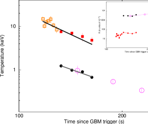
Figure 1: Evolution of the thermal components in the falling part of the last pulse of GRB 090618 is shown. The symbols are: (i) open squares denote the temperature of the BBPL model fitted to the BAT-GBM joint data, (ii) open circles denote the temperature of the BBPL model fitted to the XRT data (from Page et al. 2011), (iii) filled squares and filled circles denote the temperatures of the higher and lower temperature blackbodies obtained by 2BBPL model fitted to the joint BAT-XRT data. It is evident that the evolution of the higher temperature blackbody is similar to case (i), while the evolution of the lower temperature blackbody is similar to case (ii). Hence, the two blackbodies are always present and shows up in two different detectors (BAT and XRT) in the overlapping observation. The inset shows the evolution of $\cal{R}$, which is a proxy of the photospheric radius, for the two components. A smooth evolution is seen (see text for explanation).

This annexure gives updated information we have obtained by re-analyzing the data presented in Section 6.10. A comparison of the fit statistics of the 2BBPL and BBPL model fitted to the time-resolved BAT-GBM joint data (Table 6.5) shows that the 2BBPL model is not required based on the $\chi^{2}_{\rm red}$ values. However, when we fit the joint BAT-XRT data in the overlapping region (125-165 s) a 2BBPL model is required at a high significance ($\chi^{2}$ for BBPL and 2BBPL: 787.0 (283) and 307.1 (281), respectively). As the flux evolution in this overlapping observation has a sharp variation, we have re-analyzed the data by using finer time bins (four uniform bin in 125-165 s). The data is fitted with 2BBPL model. The temperature of the two blackbodies are shown graphically in Figure 1. The filled squares represent the higher temperature blackbody, while the filled circles represent the lower temperature blackbody. The time-resolved data before the XRT observation is fitted with a BBPL model, and the corresponding temperature is shown by open squares. The temperature of the blackbody found in the XRT data (from Page et al. 2011) are also shown (open circles). Note that the temperature of both the blackbodies of the 2BBPL model are consistent with those of the single blackbodies found in the higher (BAT/GBM) and lower energy (XRT) detectors. Hence, we conclude that the two blackbodies are always present in the data. The low blackbody is not visible in the early data because it is outside the lowest energy coverage of the higher energy detectors, and the XRT observation is absent during this time. We have also calculated the $\cal{R}$, which is a proxy of the photospheric radius, for both the components. The evolutions are shown in the inset of Figure 1. The photosphere of the lower temperature blackbody is about 65 times higher than the higher temperature blackbody. From this ratio, one finds that the required ratio of the coasting bulk Lorentz factor ($\eta$) of the spine and sheath is $\sim 8$, provided that the jet luminosity scales with $\eta$.

Chapter 9 A Few Acronyms

Appendix 9.A Astrophysical Objects

BH	Blackhole
GRB	Gamma-Ray Burst
LGRB	Long Gamma-Ray Burst
SGRB	Short Gamma-Ray Burst
NS	Neutron Star
SN	Supernova

Appendix 9.B Timing And Spectral Features

LC	Lightcurve
FRED	Fast Rise Exponential Decay
BB	Blackbody
PL	Power-law
2BBPL	Two blackbodies and a power-law
mBBPL	Multicolour blackbody and a power-law
HTS	Hard-to-soft
IT	Intensity Tracking
IC	Inverse Compton
IS	Internal Shock
ES	External Shock

Appendix 9.C General Astronomy

CCD	Charge Coupled Device
FITS	Flexible Image Transport System
FOV	Field Of View
FWHM	Full Width at Half Maximum
HEASARC	High Energy Astrophysics Science Archive Research Center
PSF	Point Spread Function
PHA	Pulse Height Amplitude
TTE	Time-tagged Event

Appendix 9.D Instruments And Missions

CGRO	Compton Gamma Ray Observatory
BATSE	Burst and Transient Source Experiment
EGRET	Energetic Gamma Ray Experiment Telescope
FGST	Fermi Gamma-ray Space Telescope
GBM	Gamma-ray Burst Monitor
LAT	Large Area Telescope
MIDEX	Medium Explorer Program
BAT	Burst Alert Telescope
XRT	X-ray Telescope
UVOT	Ultraviolet/Optical Telescope
MET	Mission Elapsed Time

References

- Abbott et al. (2008) Abbott, B., Abbott, R., Adhikari, R., et al. 2008, ApJ, 681, 1419
- Abdo et al. (2009a) Abdo, A. A., Ackermann, M., Ajello, M., et al. 2009a, Nature, 462, 331
- Abdo et al. (2009b) —. 2009b, ApJ, 706, L138
- Abdo et al. (2009c) Abdo, A. A., Ackermann, M., Arimoto, M., et al. 2009c, Science, 323, 1688
- Abdo et al. (2009d) Abdo, A. A., Ackermann, M., Ajello, M., et al. 2009d, ApJS, 183, 46
- Ackermann et al. (2010a) Ackermann, M., Asano, K., Atwood, W. B., et al. 2010a, ApJ, 716, 1178
- Ackermann et al. (2010b) Ackermann, M., Ajello, M., Baldini, L., et al. 2010b, ApJ, 717, L127
- Ackermann et al. (2011) Ackermann, M., Ajello, M., Asano, K., et al. 2011, ApJ, 729, 114
- Ackermann et al. (2013) —. 2013, ApJS, 209, 11
- Ackermann et al. (2014) —. 2014, Science, 343, 42
- Akerlof et al. (2011) Akerlof, C. W., Zheng, W., Pandey, S. B., & McKay, T. A. 2011, ApJ, 726, 22
- Aloy et al. (2000) Aloy, M. A., Müller, E., Ibáñez, J. M., Martí, J. M., & MacFadyen, A. 2000, ApJ, 531, L119
- Amati (2006) Amati, L. 2006, MNRAS, 372, 233
- Amati et al. (2009) Amati, L., Frontera, F., & Guidorzi, C. 2009, A&A, 508, 173
- Amati et al. (2002) Amati, L., Frontera, F., Tavani, M., et al. 2002, A&A, 390, 81
- Arnaud (1996) Arnaud, K. A. 1996, in Astronomical Society of the Pacific Conference Series, Vol. 101, Astronomical Data Analysis Software and Systems V, ed. G. H. Jacoby & J. Barnes, 17
- Atwood et al. (2009) Atwood, W. B., Abdo, A. A., Ackermann, M., et al. 2009, ApJ, 697, 1071
- Axelsson et al. (2012) Axelsson, M., Baldini, L., Barbiellini, G., et al. 2012, ApJ, 757, L31
- Azzam (2012) Azzam, W. J. 2012, International Journal of Astronomy and Astrophysics, 2, 1
- Band et al. (1993) Band, D., Matteson, J., Ford, L., et al. 1993, ApJ, 413, 281
- Band & Preece (2005) Band, D. L., & Preece, R. D. 2005, ApJ, 627, 319
- Barkov & Komissarov (2008) Barkov, M. V., & Komissarov, S. S. 2008, MNRAS, 385, L28
- Barnes & Kasen (2013) Barnes, J., & Kasen, D. 2013, ApJ, 775, 18
- Barniol Duran & Kumar (2011) Barniol Duran, R., & Kumar, P. 2011, MNRAS, 417, 1584
- Barraud et al. (2005) Barraud, C., Daigne, F., Mochkovitch, R., & Atteia, J. L. 2005, A&A, 440, 809
- Barthelmy et al. (2005a) Barthelmy, S. D., Chincarini, G., Burrows, D. N., et al. 2005a, Nature, 438, 994
- Barthelmy et al. (2005b) Barthelmy, S. D., Barbier, L. M., Cummings, J. R., et al. 2005b, Space Sci. Rev., 120, 143
- Basak & Rao (2012a) Basak, R., & Rao, A. R. 2012a, ApJ, 749, 132
- Basak & Rao (2012b) —. 2012b, ApJ, 745, 76
- Basak & Rao (2012c) Basak, R., & Rao, A. R. 2012c, in -Ray Bursts 2012 Conference (GRB 2012)
- Basak & Rao (2013a) —. 2013a, ApJ, 775, 31
- Basak & Rao (2013b) —. 2013b, ApJ, 768, 187
- Basak & Rao (2013c) —. 2013c, MNRAS, 436, 3082
- Basak & Rao (2014) —. 2014, MNRAS, 442, 419
- Beardmore & Schady (2009) Beardmore, A. P., & Schady, P. 2009, GRB Coordinates Network, 9528, 1
- Belli (1999) Belli, B. M. 1999, A&AS, 138, 415
- Beloborodov (2005) Beloborodov, A. M. 2005, ApJ, 618, L13
- Beniamini et al. (2011) Beniamini, P., Guetta, D., Nakar, E., & Piran, T. 2011, MNRAS, 416, 3089
- Berger (2009) Berger, E. 2009, ApJ, 690, 231
- Berger (2013) —. 2013, ArXiv e-prints, arXiv:1311.2603
- Berger et al. (2003a) Berger, E., Cowie, L. L., Kulkarni, S. R., et al. 2003a, ApJ, 588, 99
- Berger et al. (2013) Berger, E., Fong, W., & Chornock, R. 2013, ApJ, 774, L23
- Berger et al. (2003b) Berger, E., Kulkarni, S. R., Pooley, G., et al. 2003b, Nature, 426, 154
- Berger et al. (2005) Berger, E., Price, P. A., Cenko, S. B., et al. 2005, Nature, 438, 988
- Bhat et al. (1994) Bhat, P. N., Fishman, G. J., Meegan, C. A., et al. 1994, ApJ, 426, 604
- Bhat et al. (2012) Bhat, P. N., Briggs, M. S., Connaughton, V., et al. 2012, ApJ, 744, 141
- Bhattacharjee & Gupta (2003) Bhattacharjee, P., & Gupta, N. 2003, Astroparticle Physics, 20, 169
- Blandford & Znajek (1977) Blandford, R. D., & Znajek, R. L. 1977, MNRAS, 179, 433
- Bloom (2011) Bloom, J. S. 2011, What Are Gamma-Ray Bursts?
- Bloom et al. (2003) Bloom, J. S., Frail, D. A., & Kulkarni, S. R. 2003, ApJ, 594, 674
- Bloom et al. (2002) Bloom, J. S., Kulkarni, S. R., & Djorgovski, S. G. 2002, AJ, 123, 1111
- Bloom et al. (1999) Bloom, J. S., Sigurdsson, S., & Pols, O. R. 1999, MNRAS, 305, 763
- Bloom et al. (2006) Bloom, J. S., Prochaska, J. X., Pooley, D., et al. 2006, ApJ, 638, 354
- Boella et al. (1997) Boella, G., Butler, R. C., Perola, G. C., et al. 1997, A&AS, 122, 299
- Briggs (1995) Briggs, M. S. 1995, Ap&SS, 231, 3
- Burgess et al. (2011) Burgess, J. M., Preece, R. D., Baring, M. G., et al. 2011, ApJ, 741, 24
- Burrows et al. (2005a) Burrows, D. N., Romano, P., Falcone, A., et al. 2005a, Science, 309, 1833
- Burrows et al. (2005b) Burrows, D. N., Hill, J. E., Nousek, J. A., et al. 2005b, Space Sci. Rev., 120, 165
- Campana et al. (2006) Campana, S., Mangano, V., Blustin, A. J., et al. 2006, Nature, 442, 1008
- Cavallo & Rees (1978) Cavallo, G., & Rees, M. J. 1978, MNRAS, 183, 359
- Cenko (2009) Cenko, S. B. 2009, GRB Coordinates Network, 9513, 1
- Cenko et al. (2009) Cenko, S. B., Perley, D. A., Junkkarinen, V., et al. 2009, GRB Coordinates Network, 9518, 1
- Chandra & Frail (2012) Chandra, P., & Frail, D. A. 2012, ApJ, 746, 156
- Chincarini et al. (2005) Chincarini, G., Moretti, A., Romano, P., et al. 2005, ArXiv Astrophysics e-prints, astro-ph/0506453
- Chornock et al. (2010) Chornock, R., Soderberg, A. M., Foley, R. J., et al. 2010, Central Bureau Electronic Telegrams, 2228, 1
- Christensen et al. (2004) Christensen, L., Hjorth, J., & Gorosabel, J. 2004, A&A, 425, 913
- Cline & Desai (1976) Cline, T. L., & Desai, U. D. 1976, Ap&SS, 42, 17
- Cobb et al. (2006) Cobb, B. E., Bailyn, C. D., van Dokkum, P. G., & Natarajan, P. 2006, ApJ, 645, L113
- Cohen et al. (1997) Cohen, E., Katz, J. I., Piran, T., et al. 1997, ApJ, 488, 330
- Collazzi et al. (2012) Collazzi, A. C., Schaefer, B. E., Goldstein, A., & Preece, R. D. 2012, ApJ, 747, 39
- Connaughton (2002) Connaughton, V. 2002, ApJ, 567, 1028
- Costa et al. (1997) Costa, E., Frontera, F., Heise, J., et al. 1997, Nature, 387, 783
- Crider et al. (1999) Crider, A., Liang, E. P., Preece, R. D., et al. 1999, A&AS, 138, 401
- Crider et al. (1997) Crider, A., Liang, E. P., Smith, I. A., et al. 1997, ApJ, 479, L39
- Cucchiara et al. (2011) Cucchiara, A., Levan, A. J., Fox, D. B., et al. 2011, ApJ, 736, 7
- Cui et al. (2005) Cui, X.-H., Liang, E.-W., & Lu, R.-J. 2005, Chinese J. Astron. Astrophys., 5, 151
- Curran et al. (2008) Curran, P. A., van der Horst, A. J., & Wijers, R. A. M. J. 2008, MNRAS, 386, 859
- Dado et al. (2002) Dado, S., Dar, A., & De Rújula, A. 2002, A&A, 388, 1079
- Dado et al. (2007) —. 2007, ApJ, 663, 400
- D’Agostini (2005) D’Agostini, G. 2005, ArXiv Physics e-prints, physics/0511182
- Daigne & Mochkovitch (1998) Daigne, F., & Mochkovitch, R. 1998, MNRAS, 296, 275
- Dar (2006) Dar, A. 2006, Chinese Journal of Astronomy and Astrophysics Supplement, 6, 010000
- Dar & de Rújula (2004) Dar, A., & de Rújula, A. 2004, Phys. Rep., 405, 203
- Della Valle et al. (2006) Della Valle, M., Chincarini, G., Panagia, N., et al. 2006, Nature, 444, 1050
- Dermer et al. (2000) Dermer, C. D., Chiang, J., & Mitman, K. E. 2000, ApJ, 537, 785
- Dermer & Mitman (1999) Dermer, C. D., & Mitman, K. E. 1999, ApJ, 513, L5
- Dezalay et al. (1997) Dezalay, J.-P., Atteia, J.-L., Barat, C., et al. 1997, ApJ, 490, L17
- Dingus et al. (1998) Dingus, B. L., Catelli, J. R., & Schneid, E. J. 1998, in American Institute of Physics Conference Series, Vol. 428, Gamma-Ray Bursts, 4th Hunstville Symposium, ed. C. A. Meegan, R. D. Preece, & T. M. Koshut, 349–353
- Drenkhahn & Spruit (2002) Drenkhahn, G., & Spruit, H. C. 2002, A&A, 391, 1141
- Eichler et al. (1989) Eichler, D., Livio, M., Piran, T., & Schramm, D. N. 1989, Nature, 340, 126
- Evans et al. (2007) Evans, P. A., Beardmore, A. P., Page, K. L., et al. 2007, A&A, 469, 379
- Evans et al. (2009) —. 2009, MNRAS, 397, 1177
- Fan & Piran (2006) Fan, Y., & Piran, T. 2006, MNRAS, 370, L24
- Fan & Piran (2008) Fan, Y.-Z., & Piran, T. 2008, Frontiers of Physics in China, 3, 306
- Fan et al. (2005) Fan, Y. Z., Zhang, B., & Wei, D. M. 2005, ApJ, 629, 334
- Fenimore & Ramirez-Ruiz (2000) Fenimore, E. E., & Ramirez-Ruiz, E. 2000, ArXiv Astrophysics e-prints, astro-ph/0004176
- Fenimore et al. (1988) Fenimore, E. E., Conner, J. P., Epstein, R. I., et al. 1988, ApJ, 335, L71
- Firmani et al. (2006) Firmani, C., Avila-Reese, V., Ghisellini, G., & Ghirlanda, G. 2006, MNRAS, 372, L28
- Firmani et al. (2007) —. 2007, Rev. Mexicana Astron. Astrofis., 43, 203
- Firmani et al. (2005) Firmani, C., Ghisellini, G., Ghirlanda, G., & Avila-Reese, V. 2005, MNRAS, 360, L1
- Fishman (1979) Fishman, G. J. 1979, ApJ, 233, 851
- Fishman (1999) —. 1999, A&AS, 138, 395
- Fishman & Meegan (1995) Fishman, G. J., & Meegan, C. A. 1995, ARA&A, 33, 415
- Fishman et al. (1994) Fishman, G. J., Meegan, C. A., Wilson, R. B., et al. 1994, ApJS, 92, 229
- Fong et al. (2010) Fong, W., Berger, E., & Fox, D. B. 2010, ApJ, 708, 9
- Ford et al. (1995) Ford, L. A., Band, D. L., Matteson, J. L., et al. 1995, ApJ, 439, 307
- Fox et al. (2005) Fox, D. B., Frail, D. A., Price, P. A., et al. 2005, Nature, 437, 845
- Frail et al. (1994) Frail, D. A., Goss, W. M., & Whiteoak, J. B. Z. 1994, ApJ, 437, 781
- Frail et al. (2001) Frail, D. A., Kulkarni, S. R., Sari, R., et al. 2001, ApJ, 562, L55
- Fruchter et al. (1999) Fruchter, A. S., Thorsett, S. E., Metzger, M. R., et al. 1999, ApJ, 519, L13
- Fruchter et al. (2006) Fruchter, A. S., Levan, A. J., Strolger, L., et al. 2006, Nature, 441, 463
- Fryer et al. (2001) Fryer, C. L., Woosley, S. E., & Heger, A. 2001, ApJ, 550, 372
- Fynbo et al. (2006) Fynbo, J. P. U., Watson, D., Thöne, C. C., et al. 2006, Nature, 444, 1047
- Gal-Yam et al. (2006) Gal-Yam, A., Fox, D. B., Price, P. A., et al. 2006, Nature, 444, 1053
- Galama et al. (1998) Galama, T. J., Vreeswijk, P. M., van Paradijs, J., et al. 1998, Nature, 395, 670
- Gao et al. (2013) Gao, H., Lei, W.-H., Zou, Y.-C., Wu, X.-F., & Zhang, B. 2013, New A Rev., 57, 141
- Gehrels & Mészáros (2012) Gehrels, N., & Mészáros, P. 2012, Science, 337, 932
- Gehrels et al. (2009) Gehrels, N., Ramirez-Ruiz, E., & Fox, D. B. 2009, ARA&A, 47, 567
- Gehrels & Razzaque (2013) Gehrels, N., & Razzaque, S. 2013, Frontiers of Physics, 8, 661
- Gehrels et al. (2004) Gehrels, N., Chincarini, G., Giommi, P., et al. 2004, ApJ, 611, 1005
- Gehrels et al. (2005) Gehrels, N., Sarazin, C. L., O’Brien, P. T., et al. 2005, Nature, 437, 851
- Gehrels et al. (2006) Gehrels, N., Norris, J. P., Barthelmy, S. D., et al. 2006, Nature, 444, 1044
- Ghirlanda et al. (2003) Ghirlanda, G., Celotti, A., & Ghisellini, G. 2003, A&A, 406, 879
- Ghirlanda et al. (2004a) Ghirlanda, G., Ghisellini, G., & Celotti, A. 2004a, A&A, 422, L55
- Ghirlanda et al. (2004b) Ghirlanda, G., Ghisellini, G., & Lazzati, D. 2004b, ApJ, 616, 331
- Ghirlanda et al. (2010a) Ghirlanda, G., Ghisellini, G., & Nava, L. 2010a, A&A, 510, L7
- Ghirlanda et al. (2010b) Ghirlanda, G., Nava, L., & Ghisellini, G. 2010b, A&A, 511, A43
- Ghirlanda et al. (2008) Ghirlanda, G., Nava, L., Ghisellini, G., Firmani, C., & Cabrera, J. I. 2008, MNRAS, 387, 319
- Ghisellini et al. (2000) Ghisellini, G., Celotti, A., & Lazzati, D. 2000, MNRAS, 313, L1
- Ghisellini et al. (2005) Ghisellini, G., Tavecchio, F., & Chiaberge, M. 2005, A&A, 432, 401
- Goldstein et al. (2011) Goldstein, A., Preece, R. D., Briggs, M. S., et al. 2011, ArXiv e-prints, arXiv:1101.2458
- Goldstein et al. (2012) Goldstein, A., Burgess, J. M., Preece, R. D., et al. 2012, ApJS, 199, 19
- Golenetskii et al. (2009) Golenetskii, S., Aptekar, R., Mazets, E., et al. 2009, GRB Coordinates Network, 9553, 1
- Golenetskii et al. (1983) Golenetskii, S. V., Mazets, E. P., Aptekar, R. L., & Ilinskii, V. N. 1983, Nature, 306, 451
- González et al. (2003) González, M. M., Dingus, B. L., Kaneko, Y., et al. 2003, Nature, 424, 749
- Goodman (1986) Goodman, J. 1986, ApJ, 308, L47
- Götz et al. (2013) Götz, D., Covino, S., Fernández-Soto, A., Laurent, P., & Bošnjak, Ž. 2013, MNRAS, 431, 3550
- Granot et al. (2010) Granot, J., for the Fermi LAT Collaboration, & the GBM Collaboration. 2010, ArXiv e-prints, arXiv:1003.2452
- Granot & Guetta (2003) Granot, J., & Guetta, D. 2003, ApJ, 598, L11
- Granot et al. (2006) Granot, J., Königl, A., & Piran, T. 2006, MNRAS, 370, 1946
- Granot et al. (1999a) Granot, J., Piran, T., & Sari, R. 1999a, ApJ, 513, 679
- Granot et al. (1999b) —. 1999b, ApJ, 527, 236
- Granot & Sari (2002) Granot, J., & Sari, R. 2002, ApJ, 568, 820
- Gruber et al. (2014) Gruber, D., Goldstein, A., Weller von Ahlefeld, V., et al. 2014, ApJS, 211, 12
- Guetta & Della Valle (2007) Guetta, D., & Della Valle, M. 2007, ApJ, 657, L73
- Guetta et al. (2011) Guetta, D., Pian, E., & Waxman, E. 2011, A&A, 525, A53
- Guiriec et al. (2011) Guiriec, S., Connaughton, V., Briggs, M. S., et al. 2011, ApJ, 727, L33
- Guiriec et al. (2013) Guiriec, S., Daigne, F., Hascoët, R., et al. 2013, ApJ, 770, 32
- Gupta & Zhang (2007) Gupta, N., & Zhang, B. 2007, MNRAS, 380, 78
- Hakkila et al. (2008) Hakkila, J., Giblin, T. W., Norris, J. P., Fragile, P. C., & Bonnell, J. T. 2008, ApJ, 677, L81
- Hakkila & Preece (2011) Hakkila, J., & Preece, R. D. 2011, ApJ, 740, 104
- Hakkila & Preece (2014) —. 2014, ApJ, 783, 88
- Harding (2001) Harding, A. K. 2001, in Supernovae and Gamma-Ray Bursts: the Greatest Explosions since the Big Bang, ed. M. Livio, N. Panagia, & K. Sahu, 121–130
- Harrison et al. (1999) Harrison, F. A., Bloom, J. S., Frail, D. A., et al. 1999, ApJ, 523, L121
- Hartmann & Epstein (1989) Hartmann, D., & Epstein, R. I. 1989, ApJ, 346, 960
- Heger et al. (2003) Heger, A., Fryer, C. L., Woosley, S. E., Langer, N., & Hartmann, D. H. 2003, ApJ, 591, 288
- Heise et al. (2001) Heise, J., Zand, J. I., Kippen, R. M., & Woods, P. M. 2001, in Gamma-ray Bursts in the Afterglow Era, ed. E. Costa, F. Frontera, & J. Hjorth, 16
- Higdon & Lingenfelter (1990) Higdon, J. C., & Lingenfelter, R. E. 1990, ARA&A, 28, 401
- Higdon et al. (1992) Higdon, J. C., Matz, S. M., Share, G. H., Messina, D. C., & Iadicicco, A. 1992, in American Institute of Physics Conference Series, Vol. 265, American Institute of Physics Conference Series, ed. W. S. Paciesas & G. J. Fishman, 89–93
- Hjorth & Bloom (2012) Hjorth, J., & Bloom, J. S. 2012, The Gamma-Ray Burst - Supernova Connection, 169–190
- Hjorth et al. (2003) Hjorth, J., Sollerman, J., Møller, P., et al. 2003, Nature, 423, 847
- Hjorth et al. (2005a) Hjorth, J., Sollerman, J., Gorosabel, J., et al. 2005a, ApJ, 630, L117
- Hjorth et al. (2005b) Hjorth, J., Watson, D., Fynbo, J. P. U., et al. 2005b, Nature, 437, 859
- Höflich et al. (2004) Höflich, P., Kumar, P., & Wheeler, J. C., eds. 2004, Cosmic explosions in three dimensions : asymmetries in supernovae and gamma-ray bursts
- Hogg & Fruchter (1999) Hogg, D. W., & Fruchter, A. S. 1999, ApJ, 520, 54
- Holland et al. (2012) Holland, S. T., De Pasquale, M., Mao, J., et al. 2012, ApJ, 745, 41
- Hoyle (1966) Hoyle, F. 1966, Nature, 209, 751
- Huang et al. (2004) Huang, Y. F., Wu, X. F., Dai, Z. G., Ma, H. T., & Lu, T. 2004, ApJ, 605, 300
- Hurley et al. (1994) Hurley, K., Dingus, B. L., Mukherjee, R., et al. 1994, Nature, 372, 652
- Ioka et al. (2006) Ioka, K., Toma, K., Yamazaki, R., & Nakamura, T. 2006, A&A, 458, 7
- Ito et al. (2013) Ito, H., Nagataki, S., Ono, M., et al. 2013, ApJ, 777, 62
- Iwamoto et al. (1998) Iwamoto, K., Mazzali, P. A., Nomoto, K., et al. 1998, Nature, 395, 672
- Jarosik et al. (2011) Jarosik, N., Bennett, C. L., Dunkley, J., et al. 2011, ApJS, 192, 14
- Jin et al. (2007) Jin, Z. P., Yan, T., Fan, Y. Z., & Wei, D. M. 2007, ApJ, 656, L57
- Kaneko et al. (2003) Kaneko, Y., Preece, R. D., & Briggs, M. S. 2003, in Bulletin of the American Astronomical Society, Vol. 35, American Astronomical Society Meeting Abstracts, 1331
- Kaneko et al. (2006) Kaneko, Y., Preece, R. D., Briggs, M. S., et al. 2006, ApJS, 166, 298
- Kann et al. (2010) Kann, D. A., Klose, S., Zhang, B., et al. 2010, ApJ, 720, 1513
- Katz (1994a) Katz, J. I. 1994a, ApJ, 432, L107
- Katz (1994b) —. 1994b, ApJ, 422, 248
- Katz (2002) —. 2002, The biggest bangs : the mystery of gamma-ray bursts, the most violent explosions in the universe
- Kippen et al. (2003) Kippen, R. M., Woods, P. M., Heise, J., et al. 2003, in American Institute of Physics Conference Series, Vol. 662, Gamma-Ray Burst and Afterglow Astronomy 2001: A Workshop Celebrating the First Year of the HETE Mission, ed. G. R. Ricker & R. K. Vanderspek, 244–247
- Klebesadel et al. (1973) Klebesadel, R. W., Strong, I. B., & Olson, R. A. 1973, ApJ, 182, L85
- Kobayashi et al. (1997) Kobayashi, S., Piran, T., & Sari, R. 1997, ApJ, 490, 92
- Kocevski & Butler (2008) Kocevski, D., & Butler, N. 2008, ApJ, 680, 531
- Kocevski & Liang (2003) Kocevski, D., & Liang, E. 2003, ApJ, 594, 385
- Kocevski et al. (2003) Kocevski, D., Ryde, F., & Liang, E. 2003, ApJ, 596, 389
- Komissarov & Barkov (2007) Komissarov, S. S., & Barkov, M. V. 2007, MNRAS, 382, 1029
- Kono et al. (2009) Kono, K., Daikyuji, A., Sonoda, E., et al. 2009, GRB Coordinates Network, 9568, 1
- Koshut et al. (1996) Koshut, T. M., Paciesas, W. S., Kouveliotou, C., et al. 1996, ApJ, 463, 570
- Kouveliotou et al. (1993) Kouveliotou, C., Meegan, C. A., Fishman, G. J., et al. 1993, ApJ, 413, L101
- Kouveliotou et al. (1992) Kouveliotou, C., Norris, J. P., Wood, K. S., et al. 1992, ApJ, 392, 179
- Kouveliotou et al. (2012) Kouveliotou, C., Wijers, R. A. M. J., & Woosley, S. 2012, Gamma-ray Bursts
- Kouveliotou et al. (1987) Kouveliotou, C., Norris, J. P., Cline, T. L., et al. 1987, ApJ, 322, L21
- Krimm et al. (2009) Krimm, H. A., Yamaoka, K., Sugita, S., et al. 2009, ApJ, 704, 1405
- Kulkarni et al. (1998) Kulkarni, S. R., Frail, D. A., Wieringa, M. H., et al. 1998, Nature, 395, 663
- Kulkarni et al. (1999) Kulkarni, S. R., Djorgovski, S. G., Odewahn, S. C., et al. 1999, Nature, 398, 389
- Kumar & Barniol Duran (2009) Kumar, P., & Barniol Duran, R. 2009, MNRAS, 400, L75
- Kumar & Barniol Duran (2010) —. 2010, MNRAS, 409, 226
- Lamb (1995) Lamb, D. Q. 1995, PASP, 107, 1152
- Lamb et al. (2005) Lamb, D. Q., Donaghy, T. Q., & Graziani, C. 2005, ApJ, 620, 355
- Laros et al. (1987) Laros, J. G., Fenimore, E. E., Klebesadel, R. W., et al. 1987, ApJ, 320, L111
- Larsson et al. (2007) Larsson, J., Levan, A. J., Davies, M. B., & Fruchter, A. S. 2007, MNRAS, 376, 1285
- Lazzati et al. (2011) Lazzati, D., Morsony, B. J., & Begelman, M. C. 2011, ApJ, 732, 34
- Lazzati et al. (2013) Lazzati, D., Morsony, B. J., Margutti, R., & Begelman, M. C. 2013, ApJ, 765, 103
- Lazzati et al. (2001) Lazzati, D., Ramirez-Ruiz, E., & Ghisellini, G. 2001, A&A, 379, L39
- Le & Dermer (2009) Le, T., & Dermer, C. D. 2009, ApJ, 700, 1026
- Le Floc’h et al. (2003) Le Floc’h, E., Duc, P.-A., Mirabel, I. F., et al. 2003, A&A, 400, 499
- Leibler & Berger (2010) Leibler, C. N., & Berger, E. 2010, ApJ, 725, 1202
- Li & Dermer (1992) Li, H., & Dermer, C. D. 1992, Nature, 359, 514
- Li & Fenimore (1996) Li, H., & Fenimore, E. E. 1996, ApJ, 469, L115
- Li (2007) Li, L.-X. 2007, MNRAS, 379, L55
- Li & Paczyński (1998) Li, L.-X., & Paczyński, B. 1998, ApJ, 507, L59
- Li et al. (2011) Li, W., Chornock, R., Leaman, J., et al. 2011, MNRAS, 412, 1473
- Liang & Kargatis (1996) Liang, E., & Kargatis, V. 1996, Nature, 381, 49
- Liang & Dai (2004) Liang, E. W., & Dai, Z. G. 2004, ApJ, 608, L9
- Liang et al. (2008) Liang, E.-W., Racusin, J. L., Zhang, B., Zhang, B.-B., & Burrows, D. N. 2008, ApJ, 675, 528
- Liang et al. (2002) Liang, E.-W., Xie, G.-Z., & Su, C.-Y. 2002, PASJ, 54, 1
- Lipunov et al. (2001) Lipunov, V. M., Postnov, K. A., & Prokhorov, M. E. 2001, Astronomy Reports, 45, 236
- Lister et al. (2009) Lister, M. L., Cohen, M. H., Homan, D. C., et al. 2009, AJ, 138, 1874
- Liu & Wang (2011) Liu, R.-Y., & Wang, X.-Y. 2011, ApJ, 730, 1
- Lloyd & Petrosian (2000) Lloyd, N. M., & Petrosian, V. 2000, ApJ, 543, 722
- Longo et al. (2009) Longo, F., Moretti, E., Barbiellini, G., et al. 2009, GRB Coordinates Network, 9524, 1
- Lu et al. (2012) Lu, R.-J., Wei, J.-J., Liang, E.-W., et al. 2012, ApJ, 756, 112
- Lundman et al. (2014) Lundman, C., Pe’er, A., & Ryde, F. 2014, MNRAS, 440, 3292
- MacFadyen & Woosley (1999) MacFadyen, A. I., & Woosley, S. E. 1999, ApJ, 524, 262
- MacFadyen et al. (2001) MacFadyen, A. I., Woosley, S. E., & Heger, A. 2001, ApJ, 550, 410
- Macklin (1982) Macklin, J. T. 1982, MNRAS, 199, 1119
- Malesani et al. (2004) Malesani, D., Tagliaferri, G., Chincarini, G., et al. 2004, ApJ, 609, L5
- Malesani et al. (2012) Malesani, D., Schulze, S., Kruehler, T., et al. 2012, Central Bureau Electronic Telegrams, 3100, 1
- Mallozzi et al. (1995) Mallozzi, R. S., Paciesas, W. S., Pendleton, G. N., et al. 1995, ApJ, 454, 597
- Mazets & Golenetskii (1981) Mazets, E. P., & Golenetskii, S. V. 1981, Astrophysics and Space Physics Reviews, 1, 205
- Mazets et al. (1980) Mazets, E. P., Golenetskii, S. V., Aptekar, R. L., Guryan, Y. A., & Ilinskii, V. N. 1980, Soviet Astronomy Letters, 6, 372
- Mazets et al. (1979) Mazets, E. P., Golentskii, S. V., Ilinskii, V. N., Aptekar, R. L., & Guryan, I. A. 1979, Nature, 282, 587
- Mazure & Basa (2009) Mazure, A., & Basa, S. 2009, Exploding Superstars Understanding Supernovae and Gamma-Ray Bursts, doi:10.1007/978-0-387-09548-6
- Mazzali et al. (2006) Mazzali, P. A., Deng, J., Nomoto, K., et al. 2006, Nature, 442, 1018
- McBreen et al. (1994) McBreen, B., Hurley, K. J., Long, R., & Metcalfe, L. 1994, MNRAS, 271, 662
- McBreen (2009) McBreen, S. 2009, GRB Coordinates Network, 9535, 1
- McKinney (2005) McKinney, J. C. 2005, ApJ, 630, L5
- McKinney (2006) —. 2006, MNRAS, 368, 1561
- McKinney & Narayan (2007) McKinney, J. C., & Narayan, R. 2007, MNRAS, 375, 513
- Medvedev & Loeb (1999) Medvedev, M. V., & Loeb, A. 1999, ApJ, 526, 697
- Meegan et al. (1994) Meegan, C., Fishman, G., Wilson, R., et al. 1994, in American Institute of Physics Conference Series, Vol. 307, Gamma-Ray Bursts, ed. G. J. Fishman, 3
- Meegan et al. (2009) Meegan, C., Lichti, G., Bhat, P. N., et al. 2009, ApJ, 702, 791
- Mészáros (2001) Mészáros, P. 2001, Science, 291, 79
- Mészáros (2002) —. 2002, ARA&A, 40, 137
- Mészáros (2006) —. 2006, Reports on Progress in Physics, 69, 2259
- Meszaros & Rees (1993) Meszaros, P., & Rees, M. J. 1993, ApJ, 405, 278
- Meszaros & Rees (1994) —. 1994, MNRAS, 269, L41
- Mészáros & Rees (1997) Mészáros, P., & Rees, M. J. 1997, ApJ, 476, 232
- Mészáros & Rees (2001) —. 2001, ApJ, 556, L37
- Mészáros & Rees (2011) —. 2011, ApJ, 733, L40
- Meszaros et al. (1994) Meszaros, P., Rees, M. J., & Papathanassiou, H. 1994, ApJ, 432, 181
- Metzger (2010) Metzger, B. D. 2010, in Astronomical Society of the Pacific Conference Series, Vol. 432, New Horizons in Astronomy: Frank N. Bash Symposium 2009, ed. L. M. Stanford, J. D. Green, L. Hao, & Y. Mao, 81
- Metzger et al. (2007) Metzger, B. D., Thompson, T. A., & Quataert, E. 2007, ApJ, 659, 561
- Metzger et al. (2010) Metzger, B. D., Martínez-Pinedo, G., Darbha, S., et al. 2010, MNRAS, 406, 2650
- Metzger et al. (1997) Metzger, M. R., Djorgovski, S. G., Kulkarni, S. R., et al. 1997, Nature, 387, 878
- Miller (2007) Miller, J. M. 2007, ARA&A, 45, 441
- Mirabal et al. (2006) Mirabal, N., Halpern, J. P., An, D., Thorstensen, J. R., & Terndrup, D. M. 2006, ApJ, 643, L99
- Mizuta et al. (2011) Mizuta, A., Nagataki, S., & Aoi, J. 2011, ApJ, 732, 26
- Mizuta et al. (2006) Mizuta, A., Yamasaki, T., Nagataki, S., & Mineshige, S. 2006, ApJ, 651, 960
- Modjaz et al. (2006) Modjaz, M., Stanek, K. Z., Garnavich, P. M., et al. 2006, ApJ, 645, L21
- Modjaz et al. (2008) Modjaz, M., Kewley, L., Kirshner, R. P., et al. 2008, AJ, 135, 1136
- Morsony et al. (2007) Morsony, B. J., Lazzati, D., & Begelman, M. C. 2007, ApJ, 665, 569
- Mundell et al. (2013) Mundell, C. G., Kopač, D., Arnold, D. M., et al. 2013, Nature, 504, 119
- Murakami et al. (1988) Murakami, T., Fujii, M., Hayashida, K., Itoh, M., & Nishimura, J. 1988, Nature, 335, 234
- Nagataki (2009) Nagataki, S. 2009, ApJ, 704, 937
- Nakar & Piran (2002) Nakar, E., & Piran, T. 2002, MNRAS, 331, 40
- Nakar & Piran (2005) —. 2005, MNRAS, 360, L73
- Narayan et al. (1992) Narayan, R., Paczynski, B., & Piran, T. 1992, ApJ, 395, L83
- Nava et al. (2011) Nava, L., Ghirlanda, G., Ghisellini, G., & Celotti, A. 2011, A&A, 530, A21
- Nava et al. (2012) Nava, L., Salvaterra, R., Ghirlanda, G., et al. 2012, MNRAS, 421, 1256
- Nemiroff (1994) Nemiroff, R. J. 1994, Comments on Astrophysics, 17, 189
- Nemiroff (2000) —. 2000, ApJ, 544, 805
- Nolan et al. (2012) Nolan, P. L., Abdo, A. A., Ackermann, M., et al. 2012, ApJS, 199, 31
- Norris (2002) Norris, J. P. 2002, ApJ, 579, 386
- Norris & Bonnell (2006) Norris, J. P., & Bonnell, J. T. 2006, ApJ, 643, 266
- Norris et al. (2005) Norris, J. P., Bonnell, J. T., Kazanas, D., et al. 2005, ApJ, 627, 324
- Norris et al. (2000) Norris, J. P., Marani, G. F., & Bonnell, J. T. 2000, ApJ, 534, 248
- Norris et al. (1996) Norris, J. P., Nemiroff, R. J., Bonnell, J. T., et al. 1996, ApJ, 459, 393
- Norris et al. (1986) Norris, J. P., Share, G. H., Messina, D. C., et al. 1986, ApJ, 301, 213
- Nousek & Shue (1989) Nousek, J. A., & Shue, D. R. 1989, ApJ, 342, 1207
- Nousek et al. (2006) Nousek, J. A., Kouveliotou, C., Grupe, D., et al. 2006, ApJ, 642, 389
- O’Brien et al. (2006) O’Brien, P. T., Willingale, R., Osborne, J., et al. 2006, ApJ, 647, 1213
- Ofek et al. (2008) Ofek, E. O., Muno, M., Quimby, R., et al. 2008, ApJ, 681, 1464
- Ogasaka et al. (1991) Ogasaka, Y., Murakami, T., Nishimura, J., Yoshida, A., & Fenimore, E. E. 1991, ApJ, 383, L61
- Paciesas et al. (2012) Paciesas, W. S., Meegan, C. A., von Kienlin, A., et al. 2012, ApJS, 199, 18
- Paczynski (1986) Paczynski, B. 1986, ApJ, 308, L43
- Paczynski (1991) —. 1991, Acta Astron., 41, 257
- Paczynski (1992) —. 1992, Acta Astron., 42, 145
- Paczynski (1995) —. 1995, PASP, 107, 1167
- Paczyński (1998a) Paczyński, B. 1998a, ApJ, 494, L45
- Paczyński (1998b) Paczyński, B. 1998b, in American Institute of Physics Conference Series, Vol. 428, Gamma-Ray Bursts, 4th Hunstville Symposium, ed. C. A. Meegan, R. D. Preece, & T. M. Koshut, 783–787
- Page et al. (2011) Page, K. L., Starling, R. L. C., Fitzpatrick, G., et al. 2011, MNRAS, 416, 2078
- Palmer et al. (2005) Palmer, D. M., Barthelmy, S., Gehrels, N., et al. 2005, Nature, 434, 1107
- Panaitescu (2007) Panaitescu, A. 2007, MNRAS, 379, 331
- Panaitescu (2008) —. 2008, MNRAS, 385, 1628
- Panaitescu & Kumar (2000) Panaitescu, A., & Kumar, P. 2000, ApJ, 543, 66
- Panaitescu et al. (2001) Panaitescu, A., Kumar, P., & Narayan, R. 2001, ApJ, 561, L171
- Panaitescu & Mészáros (2000) Panaitescu, A., & Mészáros, P. 2000, ApJ, 544, L17
- Panaitescu et al. (2006) Panaitescu, A., Mészáros, P., Burrows, D., et al. 2006, MNRAS, 369, 2059
- Pe’er (2008) Pe’er, A. 2008, ApJ, 682, 463
- Pe’er et al. (2005) Pe’er, A., Mészáros, P., & Rees, M. J. 2005, ApJ, 635, 476
- Pe’er et al. (2006) —. 2006, ApJ, 642, 995
- Pe’er & Ryde (2011) Pe’er, A., & Ryde, F. 2011, ApJ, 732, 49
- Pe’er & Waxman (2004a) Pe’er, A., & Waxman, E. 2004a, ApJ, 613, 448
- Pe’er & Waxman (2004b) —. 2004b, ApJ, 603, L1
- Pe’er & Waxman (2005) —. 2005, ApJ, 633, 1018
- Pendleton et al. (1994) Pendleton, G. N., Paciesas, W. S., Briggs, M. S., et al. 1994, ApJ, 431, 416
- Peng et al. (2005) Peng, F., Königl, A., & Granot, J. 2005, ApJ, 626, 966
- Percival et al. (2010) Percival, W. J., Reid, B. A., Eisenstein, D. J., et al. 2010, MNRAS, 401, 2148
- Perley (2009) Perley, D. A. 2009, GRB Coordinates Network, 9514, 1
- Perlmutter et al. (1999) Perlmutter, S., Aldering, G., Goldhaber, G., et al. 1999, ApJ, 517, 565
- Perna & Belczynski (2002) Perna, R., & Belczynski, K. 2002, ApJ, 570, 252
- Pian et al. (2000) Pian, E., Amati, L., Antonelli, L. A., et al. 2000, ApJ, 536, 778
- Pian et al. (2006) Pian, E., Mazzali, P. A., Masetti, N., et al. 2006, Nature, 442, 1011
- Pilla & Loeb (1998) Pilla, R. P., & Loeb, A. 1998, ApJ, 494, L167
- Piran (1992) Piran, T. 1992, ApJ, 389, L45
- Piran (1999) —. 1999, Phys. Rep., 314, 575
- Piran (2000) —. 2000, Phys. Rep., 333, 529
- Piran (2004) —. 2004, Reviews of Modern Physics, 76, 1143
- Planck Collaboration et al. (2013) Planck Collaboration, Ade, P. A. R., Aghanim, N., et al. 2013, ArXiv e-prints, arXiv:1303.5076
- Preece et al. (1998) Preece, R. D., Briggs, M. S., Mallozzi, R. S., et al. 1998, ApJ, 506, L23
- Preece et al. (2000) —. 2000, ApJS, 126, 19
- Preece et al. (1996) Preece, R. D., Briggs, M. S., Pendleton, G. N., et al. 1996, ApJ, 473, 310
- Prochaska et al. (2006) Prochaska, J. X., Bloom, J. S., Chen, H.-W., et al. 2006, ApJ, 642, 989
- Proga et al. (2003) Proga, D., MacFadyen, A. I., Armitage, P. J., & Begelman, M. C. 2003, ApJ, 599, L5
- Proga & Zhang (2006) Proga, D., & Zhang, B. 2006, MNRAS, 370, L61
- Qin & Dong (2005) Qin, Y.-P., & Dong, Y.-M. 2005, MNRAS, 358, 1320
- Qin et al. (2000) Qin, Y.-P., Xie, G.-Z., Xue, S.-J., et al. 2000, PASJ, 52, 759
- Racusin et al. (2009) Racusin, J. L., Liang, E. W., Burrows, D. N., et al. 2009, ApJ, 698, 43
- Ramirez-Ruiz et al. (2002) Ramirez-Ruiz, E., Celotti, A., & Rees, M. J. 2002, MNRAS, 337, 1349
- Ramirez-Ruiz & Fenimore (2000) Ramirez-Ruiz, E., & Fenimore, E. E. 2000, ApJ, 539, 712
- Rao et al. (2014) Rao, A. R., Basak, R., Bhattacharya, J., et al. 2014, Research in Astronomy and Astrophysics, 14, 35
- Rao et al. (2009) Rao, A. R., Malkar, J. P., Hingar, M. K., et al. 2009, GRB Coordinates Network, 9665, 1
- Rao et al. (2011) —. 2011, ApJ, 728, 42
- Raskin et al. (2008) Raskin, C., Scannapieco, E., Rhoads, J., & Della Valle, M. 2008, ApJ, 689, 358
- Razzaque et al. (2004) Razzaque, S., Mészáros, P., & Zhang, B. 2004, ApJ, 613, 1072
- Rees (1967) Rees, M. J. 1967, MNRAS, 135, 345
- Rees & Meszaros (1992) Rees, M. J., & Meszaros, P. 1992, MNRAS, 258, 41P
- Rees & Meszaros (1994) —. 1994, ApJ, 430, L93
- Rees & Mészáros (2005) Rees, M. J., & Mészáros, P. 2005, ApJ, 628, 847
- Reichart (1997) Reichart, D. E. 1997, ApJ, 485, L57
- Reichart et al. (2001) Reichart, D. E., Lamb, D. Q., Fenimore, E. E., et al. 2001, ApJ, 552, 57
- Rhoads (1997) Rhoads, J. E. 1997, ApJ, 487, L1
- Rhoads (1999) —. 1999, ApJ, 525, 737
- Ricker et al. (2003) Ricker, G. R., Atteia, J.-L., Crew, G. B., et al. 2003, in American Institute of Physics Conference Series, Vol. 662, Gamma-Ray Burst and Afterglow Astronomy 2001: A Workshop Celebrating the First Year of the HETE Mission, ed. G. R. Ricker & R. K. Vanderspek, 3–16
- Riess et al. (1998) Riess, A. G., Filippenko, A. V., Challis, P., et al. 1998, AJ, 116, 1009
- Riess et al. (2007) Riess, A. G., Strolger, L.-G., Casertano, S., et al. 2007, ApJ, 659, 98
- Riess et al. (2011) Riess, A. G., Macri, L., Casertano, S., et al. 2011, ApJ, 730, 119
- Roming et al. (2005) Roming, P. W. A., Kennedy, T. E., Mason, K. O., et al. 2005, Space Sci. Rev., 120, 95
- Rossi et al. (2002) Rossi, E., Lazzati, D., & Rees, M. J. 2002, MNRAS, 332, 945
- Rubtsov et al. (2012) Rubtsov, G. I., Pshirkov, M. S., & Tinyakov, P. G. 2012, MNRAS, 421, L14
- Ruderman (1975) Ruderman, M. 1975, in Annals of the New York Academy of Sciences, Vol. 262, Seventh Texas Symposium on Relativistic Astrophysics, ed. P. G. Bergman, E. J. Fenyves, & L. Motz, 164–180
- Ryde (2004) Ryde, F. 2004, ApJ, 614, 827
- Ryde (2005) —. 2005, ApJ, 625, L95
- Ryde & Pe’er (2009) Ryde, F., & Pe’er, A. 2009, ApJ, 702, 1211
- Ryde et al. (2010) Ryde, F., Axelsson, M., Zhang, B. B., et al. 2010, ApJ, 709, L172
- Sakamoto et al. (2011a) Sakamoto, T., Pal’Shin, V., Yamaoka, K., et al. 2011a, PASJ, 63, 215
- Sakamoto et al. (2011b) Sakamoto, T., Barthelmy, S. D., Baumgartner, W. H., et al. 2011b, ApJS, 195, 2
- Salvaterra et al. (2009) Salvaterra, R., Della Valle, M., Campana, S., et al. 2009, Nature, 461, 1258
- Sari et al. (1996) Sari, R., Narayan, R., & Piran, T. 1996, ApJ, 473, 204
- Sari & Piran (1997) Sari, R., & Piran, T. 1997, MNRAS, 287, 110
- Sari & Piran (1999a) —. 1999a, ApJ, 517, L109
- Sari & Piran (1999b) —. 1999b, ApJ, 520, 641
- Sari et al. (1999) Sari, R., Piran, T., & Halpern, J. P. 1999, ApJ, 519, L17
- Savaglio et al. (2006) Savaglio, S., Glazebrook, K., & Le Borgne, D. 2006, in American Institute of Physics Conference Series, Vol. 836, Gamma-Ray Bursts in the Swift Era, ed. S. S. Holt, N. Gehrels, & J. A. Nousek, 540–545
- Schady (2009) Schady, P. 2009, GRB Coordinates Network, 9527, 1
- Schady et al. (2009a) Schady, P., Baumgartner, W. H., & Beardmore, A. P. 2009a, GCN Report, 232, 1
- Schady et al. (2009b) Schady, P., Baumgartner, W. H., Beardmore, A. P., et al. 2009b, GRB Coordinates Network, 9512, 1
- Schaefer (2003) Schaefer, B. E. 2003, ApJ, 583, L67
- Schaefer (2007) —. 2007, ApJ, 660, 16
- Schaefer & Collazzi (2007) Schaefer, B. E., & Collazzi, A. C. 2007, ApJ, 656, L53
- Schaefer et al. (1992) Schaefer, B. E., Teegarden, B. J., Cline, T. L., et al. 1992, ApJ, 393, L51
- Schmidt et al. (1998) Schmidt, B. P., Suntzeff, N. B., Phillips, M. M., et al. 1998, ApJ, 507, 46
- Schmidt et al. (1988) Schmidt, M., Higdon, J. C., & Hueter, G. 1988, ApJ, 329, L85
- Schmidt (1978) Schmidt, W. K. H. 1978, Nature, 271, 525
- Sekiguchi & Shibata (2011) Sekiguchi, Y., & Shibata, M. 2011, ApJ, 737, 6
- Shahmoradi (2013) Shahmoradi, A. 2013, ApJ, 766, 111
- Shemi & Piran (1990) Shemi, A., & Piran, T. 1990, ApJ, 365, L55
- Sheth et al. (2003) Sheth, K., Frail, D. A., White, S., et al. 2003, ApJ, 595, L33
- Shirasaki et al. (2008) Shirasaki, Y., Yoshida, A., Kawai, N., et al. 2008, PASJ, 60, 919
- Smith & Owocki (2006) Smith, N., & Owocki, S. P. 2006, ApJ, 645, L45
- Soderberg et al. (2006a) Soderberg, A. M., Nakar, E., Berger, E., & Kulkarni, S. R. 2006a, ApJ, 638, 930
- Soderberg et al. (2005) Soderberg, A. M., Kulkarni, S. R., Fox, D. B., et al. 2005, ApJ, 627, 877
- Soderberg et al. (2006b) Soderberg, A. M., Kulkarni, S. R., Nakar, E., et al. 2006b, Nature, 442, 1014
- Soderberg et al. (2006c) Soderberg, A. M., Berger, E., Kasliwal, M., et al. 2006c, ApJ, 650, 261
- Soderberg et al. (2010) Soderberg, A. M., Chakraborti, S., Pignata, G., et al. 2010, Nature, 463, 513
- Sollerman et al. (2006) Sollerman, J., Jaunsen, A. O., Fynbo, J. P. U., et al. 2006, A&A, 454, 503
- Spruit et al. (2001) Spruit, H. C., Daigne, F., & Drenkhahn, G. 2001, A&A, 369, 694
- Stanek et al. (1999) Stanek, K. Z., Garnavich, P. M., Kaluzny, J., Pych, W., & Thompson, I. 1999, ApJ, 522, L39
- Stanek et al. (2003) Stanek, K. Z., Matheson, T., Garnavich, P. M., et al. 2003, ApJ, 591, L17
- Stanek et al. (2006) Stanek, K. Z., Gnedin, O. Y., Beacom, J. F., et al. 2006, Acta Astron., 56, 333
- Szostek & Zdziarski (2007) Szostek, A., & Zdziarski, A. A. 2007, MNRAS, 375, 793
- Takiwaki et al. (2009) Takiwaki, T., Kotake, K., & Sato, K. 2009, ApJ, 691, 1360
- Tanvir et al. (2005) Tanvir, N. R., Chapman, R., Levan, A. J., & Priddey, R. S. 2005, Nature, 438, 991
- Tanvir et al. (2013) Tanvir, N. R., Levan, A. J., Fruchter, A. S., et al. 2013, Nature, 500, 547
- Tanvir et al. (2009) Tanvir, N. R., Fox, D. B., Levan, A. J., et al. 2009, Nature, 461, 1254
- Tavani (1997) Tavani, M. 1997, ApJ, 483, L87
- Thompson (1994) Thompson, C. 1994, MNRAS, 270, 480
- Toma et al. (2012) Toma, K., Mukohyama, S., Yonetoku, D., et al. 2012, Physical Review Letters, 109, 241104
- Totani (1998) Totani, T. 1998, ApJ, 509, L81
- Tsutsui et al. (2008) Tsutsui, R., Nakamura, T., Yonetoku, D., et al. 2008, MNRAS, 386, L33
- Tueller et al. (2010) Tueller, J., Baumgartner, W. H., Markwardt, C. B., et al. 2010, ApJS, 186, 378
- Usov (1992) Usov, V. V. 1992, Nature, 357, 472
- Usov (1994) —. 1994, MNRAS, 267, 1035
- Usov & Chibisov (1975) Usov, V. V., & Chibisov, G. V. 1975, Soviet Ast., 19, 115
- van Eerten et al. (2010) van Eerten, H., Zhang, W., & MacFadyen, A. 2010, ApJ, 722, 235
- van Paradijs et al. (2000) van Paradijs, J., Kouveliotou, C., & Wijers, R. A. M. J. 2000, ARA&A, 38, 379
- van Paradijs et al. (1997) van Paradijs, J., Groot, P. J., Galama, T., et al. 1997, Nature, 386, 686
- van Putten (2005) van Putten, M. H. P. M. 2005, Gravitational radiation, luminous black holes, and gamma-ray burst supernovae
- Vedrenne & Atteia (2009) Vedrenne, G., & Atteia, J.-L. 2009, Gamma-Ray Bursts: The brightest explosions in the Universe
- Vietri (1997) Vietri, M. 1997, ApJ, 478, L9
- Vlahakis et al. (2003) Vlahakis, N., Peng, F., & Königl, A. 2003, ApJ, 594, L23
- von Kienlin et al. (2014) von Kienlin, A., Meegan, C. A., Paciesas, W. S., et al. 2014, ApJS, 211, 13
- Wang et al. (2011) Wang, F.-Y., Qi, S., & Dai, Z.-G. 2011, MNRAS, 415, 3423
- Wang et al. (2001a) Wang, X. Y., Dai, Z. G., & Lu, T. 2001a, ApJ, 546, L33
- Wang et al. (2001b) —. 2001b, ApJ, 556, 1010
- Wang et al. (2006) Wang, X.-Y., Li, Z., & Mészáros, P. 2006, ApJ, 641, L89
- Wang et al. (2013) Wang, X.-Y., Liu, R.-Y., & Lemoine, M. 2013, ApJ, 771, L33
- Waxman (1997) Waxman, E. 1997, ApJ, 485, L5
- Weiler (2003) Weiler, K., ed. 2003, Lecture Notes in Physics, Berlin Springer Verlag, Vol. 598, Supernovae and Gamma-Ray Bursters
- Wiersema et al. (2012) Wiersema, K., Cucchiara, A., Levan, A. J., et al. 2012, GRB Coordinates Network, 13276, 1
- Wiersema et al. (2014) Wiersema, K., Covino, S., Toma, K., et al. 2014, Nature, 509, 201
- Wijers et al. (1997) Wijers, R. A. M. J., Rees, M. J., & Meszaros, P. 1997, MNRAS, 288, L51
- Willingale et al. (2006) Willingale, R., O’Brien, P. T., Cowley, S. W. H., et al. 2006, ApJ, 649, 541
- Woltjer (1966) Woltjer, L. 1966, ApJ, 146, 597
- Woods & Loeb (1995) Woods, E., & Loeb, A. 1995, ApJ, 453, 583
- Woosley (1993) Woosley, S. E. 1993, ApJ, 405, 273
- Woosley & Bloom (2006) Woosley, S. E., & Bloom, J. S. 2006, ARA&A, 44, 507
- Woosley et al. (1999) Woosley, S. E., Eastman, R. G., & Schmidt, B. P. 1999, ApJ, 516, 788
- Woosley & Heger (2006) Woosley, S. E., & Heger, A. 2006, ApJ, 637, 914
- Woosley et al. (2002) Woosley, S. E., Heger, A., & Weaver, T. A. 2002, Reviews of Modern Physics, 74, 1015
- Wu et al. (2005) Wu, X. F., Dai, Z. G., Huang, Y. F., & Lu, T. 2005, MNRAS, 357, 1197
- Xu & Li (2014) Xu, S.-Y., & Li, Z. 2014, Research in Astronomy and Astrophysics, 14, 411
- Yi et al. (2006) Yi, T., Liang, E., Qin, Y., & Lu, R. 2006, MNRAS, 367, 1751
- Yonetoku et al. (2004) Yonetoku, D., Murakami, T., Nakamura, T., et al. 2004, ApJ, 609, 935
- Yonetoku et al. (2010) Yonetoku, D., Murakami, T., Tsutsui, R., et al. 2010, PASJ, 62, 1495
- Yonetoku et al. (2012) Yonetoku, D., Murakami, T., Gunji, S., et al. 2012, ApJ, 758, L1
- Zhang (2007a) Zhang, B. 2007a, Advances in Space Research, 40, 1186
- Zhang (2007b) —. 2007b, Chinese J. Astron. Astrophys., 7, 1
- Zhang (2014) —. 2014, International Journal of Modern Physics D, 23, 30002
- Zhang et al. (2004a) Zhang, B., Dai, X., Lloyd-Ronning, N. M., & Mészáros, P. 2004a, ApJ, 601, L119
- Zhang et al. (2006) Zhang, B., Fan, Y. Z., Dyks, J., et al. 2006, ApJ, 642, 354
- Zhang & Mészáros (2001) Zhang, B., & Mészáros, P. 2001, ApJ, 559, 110
- Zhang & Mészáros (2002) —. 2002, ApJ, 581, 1236
- Zhang & Mészáros (2004) —. 2004, International Journal of Modern Physics A, 19, 2385
- Zhang & Pe’er (2009) Zhang, B., & Pe’er, A. 2009, ApJ, 700, L65
- Zhang & Yan (2011) Zhang, B., & Yan, H. 2011, ApJ, 726, 90
- Zhang et al. (2007a) Zhang, B., Zhang, B.-B., Liang, E.-W., et al. 2007a, ApJ, 655, L25
- Zhang et al. (2007b) Zhang, B., Liang, E., Page, K. L., et al. 2007b, ApJ, 655, 989
- Zhang et al. (2014) Zhang, B.-B., van Eerten, H., Burrows, D. N., et al. 2014, ArXiv e-prints, arXiv:1405.4867
- Zhang et al. (2011) Zhang, B.-B., Zhang, B., Liang, E.-W., et al. 2011, ApJ, 730, 141
- Zhang et al. (2004b) Zhang, W., Woosley, S. E., & Heger, A. 2004b, ApJ, 608, 365
- Zhang et al. (2003) Zhang, W., Woosley, S. E., & MacFadyen, A. I. 2003, ApJ, 586, 356
- Zheng et al. (2012) Zheng, W., Akerlof, C. W., Pandey, S. B., et al. 2012, ApJ, 756, 64