Towards an $N$-body Model for the Globular Cluster M4

Abstract

This paper describes an $N$-body model for the dynamical evolution of the nearby globular cluster M4. The initial conditions, with $N=484710$ particles, were generated from a published study of this cluster with a Monte Carlo code. With the Monte Carlo code, these initial conditions led, after 12 Gyr of dynamical and stellar evolution, to a model which resembles M4 in terms of its surface brightness and velocity dispersion profiles, and its local luminosity function. Though the $N$-body  model reported here is marred by some errors, its evolution can be compared with that of the published Monte Carlo model, with a result from the synthetic evolution code EMACSS, and with M4 itself.

1 Introduction

Globular star clusters are an obvious target for modelling by $N$-body simulations. Software techniques have been developed over several decades, and are well matched to readily available current hardware (Aarseth, 1999; Nitadori & Aarseth, 2012). And yet progress in applying these methods to the Galactic globular clusters has been very slow, simply because the computations take such a long time. Indeed only two clusters have been adequately modelled, in the sense that initial conditions have been selected so that the evolved model matches detailed observational data on the cluster. These are the clusters Pal 14 and Pal 4 (Hasani Zonoozi et al., 2011, 2014). These are manageable because the initial particle number ($\mathrel{\raise 1.29167pt\hbox{$<$}\mkern-14.0mu\lower 2.58334pt\hbox{$\sim$}}10^{5}$) is not excessive, and the initial models are relatively distended (half-mass radius $\mathrel{\raise 1.29167pt\hbox{$>$}\mkern-14.0mu\lower 2.58334pt\hbox{$\sim$}}10$pc), making all time-scales relatively large, and the computations short.

Without such restrictions (i.e. for the bulk of the Galactic globular clusters, and certainly the richer and best observed ones) one must resort to approximate modelling techniques. One of these is to use small $N$-body models, i.e. models in which the number of stars is much smaller than that in the actual cluster under study, and to scale the results appropriately, which means scaling so that the relaxation time of the model matches that of the real cluster. An alternative is the use of a Monte Carlo code (Giersz, 1998; Joshi, Rasio, & Portegies Zwart, 2000; Fregeau & Rasio, 2007; Giersz et al., 2013), which yields results much more quickly than even a scaled $N$-body model, but with a different set of simplifying approximations. Both of these approximate methods have been used, for example, to study the dynamics of stellar-mass black holes in the cluster M22 (Sippel & Hurley, 2013; Heggie & Giersz, 2014).

Experience shows that finding appropriate initial conditions in such studies requires the computation of order 50 models or more. Therefore the speed of the Monte Carlo method, which can compute each model in a day or two, is a major advantage, except for the sparsest clusters. For this reason it has been used in a number of studies of the richest, closest and best observed clusters (Heggie & Giersz, 2008; Giersz & Heggie, 2009, 2011; Heggie & Giersz, 2014), of which the first was M4. This is the nearest Galactic globular cluster, which makes it uniquely favourable for the most delicate observational programmes (e.g. Bedin et al., 2013).

The current mass of M4 has been estimated at about $10^{5}M_{\odot}$ (McLaughlin & van der Marel, 2005), which seems roughly comparable with Pal 4 and Pal 14. But two factors make it a harder target for $N$-body modelling: its smaller half-mass radius (under 1pc initially, according to Heggie & Giersz (2008)), which reduces the time scale of its evolution, and the likelihood that it has lost a large fraction of its population. Indeed the best fitting models which were found by Heggie & Giersz (2008) were those which began with almost $5\times 10^{5}$ stars. Nevertheless the continuing importance of this object, and the availability of appropriate initial conditions from the Monte Carlo study, motivated the author to attempt a direct $N$-body simulation.

The description of this model and results, and comparison with two approximate models (mainly, the Monte Carlo model) and observational data on M4 are the main purposes of this paper. The following section summarises the initial conditions, and software and hardware issues, including difficulties and flaws in the model. Section 3 presents the main results on the dynamical evolution of the model, and a comparison with the Monte Carlo results. A comparison with observations of the cluster itself is the topic of Section 4. The final section picks out some highlights, and sums up.

2 Description of the simulation

2.1 Initial conditions, software and hardware

Initial conditions were generated from those of a Monte Carlo model described by Heggie & Giersz (2008, Tables 1 and 3). Briefly, the initial model is a Plummer model, with initial tidal and half-mass radii of 35.0 and 0.58 pc, respectively. The tidal field was that of a point-mass galaxy. The initial number of objects (single stars plus binaries) was 453000, of which 7% were binaries. Thus the initial number of stars was 484710. The initial mass function for single stars was a continuous, two-part power law in the range $0.1M_{\odot}<m<50M_{\odot}$, with power law indices of 0.9 and 2.3 (Salpeter) below and above a break mass of $0.5M_{\odot}$. The binary mass distribution was drawn from Kroupa, Gilmore, & Tout (1991, eq.1), with a uniform mass ratio between components, restricted to component masses in the same range as for single stars. A uniform distribution for the log of the semi-major axis in the range from 50AU down to twice the sum of the radii of the components was used. Eccentricities were thermal, with “eigenevolution” (Kroupa, 1995). The stellar metallicity was $Z=0.002$. As a result of these choices the units of mass and time (Hénon units) were, respectively, $350044M_{\odot}$ (the initial total mass) and $0.01655$Myr, reflecting the short initial crossing time of the model.

The initial conditions of the Monte Carlo model are incomplete for $N$-body purposes (e.g. the initial position of a star is specified only as far as the radius), and complete $N$-body initial conditions were generated using the obvious distributions. For single stars and the barycentres of binaries, the spherical polar angles of the position are distributed with probability density function $f(\theta,\phi)=\sin\theta/(4\pi)$. Given the magnitude of the radial and transverse components of the velocity (of a single star or binary barycentre), the sign of the radial velocity is chosen with probability $0.5$ each, and the direction of the transverse component is specified by an angle $\psi$ (in a plane perpendicular to the radius vector) with probability density $f(\psi)=1/(2\pi)$. For each binary the semi-major axis, $a$, and eccentricity, $e$, are known from the Monte Carlo data. The three standard angles specifying the orientation of the binary orbit (i.e. the orbit for the relative motion of the two components) is chosen from $f(\omega,\Omega,i)=\sin i/(8\pi^{2})$, and the initial mean anomaly has probability density $f(M)=1/(2\pi)$.

The simulation was run on two virtually identical devices (fermi0 and fermi1, which were used alternately according to availability) at Edinburgh Parallel Computing Centre. Each is equipped with $4\times 6$ Intel Xeon X5650 cores at 2.67GHz, and 4 Nvidia Tesla C2050 GPUs, though, as these are shared machines, only 12 cores and 2 cards were used for this simulation.

The simulation was carried out with the code NBODY6 in a form which exploits GPUs (Nitadori & Aarseth, 2012). As this code is continually evolving and improving, however, several different versions were adopted during the long course of the run. In some cases the version was changed in order to progress over a particularly recalcitrant problem in the simulation.

Output was mainly confined to a quite full version of the standard output of NBODY6, sampled every Hénon time unit initially, and then more infrequently as the simulation speeded up. A complete dump of the calculation, from which a restart would be possible, was taken almost daily. Particle lists extracted from these dumps are available at http://datashare.is.ed.ac.uk/handle/10283/618 .

2.2 Progress of the simulation

The simulation began in October 2010 and was finally completed after 2 years and 8 months in June 2013. Only about 5 months were unproductive, because of downtime and the occasional need for restarts. The effort devoted to different parts of the simulation varied enormously, as can be seen from Fig.1. To begin with each Hénon time unit took about 3 hours, at which rate the entire simulation would have taken nearly 400 years. As shall be seen (Sec.3.1.2) an expansion of the system began around 5 Myr, and then the wall-clock time per Hénon unit began to diminish. The decrease accelerated in the latter part of the simulation because of escape.

Figure 1: Wall-clock time in hours per Hénon time unit, as a function of simulated evolution time in Myr.

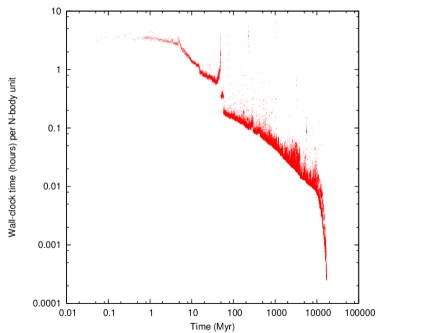
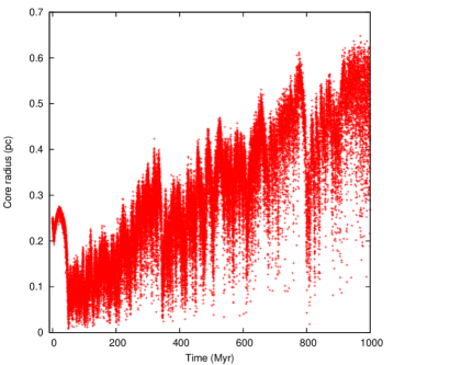
Between the early and late phases of the simulation only two features are noteworthy. At around 50 Myr a sharp deterioration in performance was noted (see Fig.1), accompanied by collapse of a core consisting predominantly of stellar-mass black holes (Fig.6,which shows the early evolution of the core radius). On inspection a decrease was noticed in the regularisation parameters $R_{cl}$ and $\Delta t_{cl}$ (Aarseth, 2003, p.145), caused by a specific choice of a certain NBODY6 input parameter. When corrected, the rate of progress improved by about a factor of 10. The second feature, visible above and to the right of the “main sequence” of points in Fig.1, is a number of phases of poor performance caused by “difficult” few-body interactions, when the time taken per Hénon time unit can increase by as much as a factor of 100.

2.3 Anomalies

2.3.1 Roche-lobe treatment

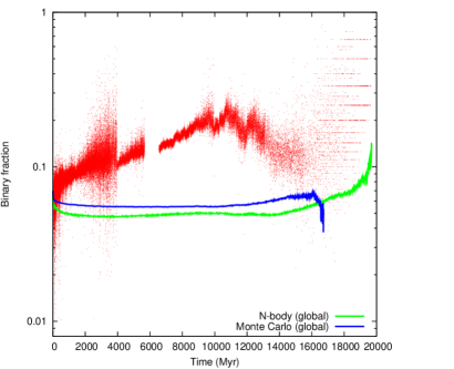
During the course of the run, two flaws emerged which have a significant effect on some of the statistical results of interest. The first concerns binaries, and resulted from a recalcitrant error in the treatment of one case of Roche-lobe overflow. Different treatments of this process are available in NBODY6, and again a change of one input parameter cured the problem. However, this also apparently led to a slight decrease in the binary fraction, from about 4.82% to about 4.79%. This is invisible on the scale of Fig.7, where the binary fraction is plotted.

2.3.2 “Anomalous” black holes

Much more serious was a flaw which was noticed when, just before 4 Gyr, the total bound mass of the model decreased by several hundred solar masses between successive output times. After some time this was traced to an unfortunate choice of one of the starting parameters in NBODY6. The result of this flaw was to artificially enhance the rate of collisions of neutron stars and black holes with other objects, and hence (in particular) it led to the build-up of the mass of individual black holes. Its effects, which are discussed further below (Sections 3.1.2, 3.2 and 3.3.2), are particularly noticeable in the measurements of the core radius.

A list of the detected anomalous black holes is given in Table 1, and for brevity these objects are referred to henceforth as ABH1, etc, using the identifier in this table. In most of the early cases each object was involved in only one event, at the time stated. All except the last, which was still present when the simulation ended, presumably escaped. It may seem surprising that such a massive object as ABH23 can escape dynamically, but it was not the only anomalous black hole present at the time, and interactions between these two objects and normal black holes may be responsible. Unfortunately no details of such interactions were stored.

Table 1: Detected “anomalous” black holes

Identifier	First detection	Last detection	Final Mass
	(Myr)	(Myr)	($M_{\odot}$)
1	106.2	106.2	33.4
2	106.5	106.5	37.9
3	107.1	107.1	38.8
4	107.2	107.2	38.6
5	206.9	206.9	38.6
6	207.2	207.2	38.9
7	207.3	207.3	38.9
8	207.4	317.4	110.3
9	306.4	306.4	38.6
10	371.8	371.8	14.3
11	405.4	405.4	33.3
12	406.2	406.2	34.5
13	505.5	505.5	37.8
14	506.2	506.2	38.2
15	507.0	606.2	58.3
16	663.4	663.4	19.8
17	704.6	704.6	29.0
18	705.1	705.1	38.4
19	705.5	705.5	38.8
20	706.5	706.5	38.5
21	814.1	814.1	19.6
22	836.0	1213.7	189.0
23	1213.7	3957.0	514.5
24	3946.8	5512.8	155.8
25	6188.8	9908.7	66.9
26	10453.9	10987.9	22.0
27	10686.9	11843.3	26.8
28	12478.0	12670.0	11.4
29	13376.8	19550.6	114.6

3 Results of the model

In this description of the results a comparison is given, where possible, with the Monte Carlo simulation of Heggie & Giersz (2008), though it is worth mentioning here that the Monte Carlo code has been substantially developed since the time of that study (see Giersz et al., 2013). A comparison is also presented with the synthetic cluster evolution code EMACSS (Alexander et al., 2014).

3.1 Global evolution

3.1.1 Total mass

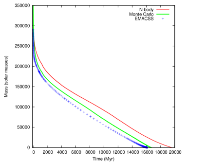
The evolution of the mass within the tidal radius is shown in Fig.2. All models exhibit the familiar two stages of mass loss: first, a rapid loss through winds and supernovae (mainly), and, second, a gentler loss due to escape across the tidal boundary.

In the first stage, it might be thought surprising that the Monte Carlo model loses mass more rapidly than the $N$-body  model, as both codes use the same packages for stellar evolution (Hurley, Pols, & Tout, 2000; Hurley, Tout, & Pols, 2002). But the treatment of escape in the Monte Carlo model is deliberately generous: the escape energy is lowered a little in order to match in a crude way the complicated physics of escape in a tidal field (Giersz, Heggie, & Hurley, 2008, Sec.2.2.2). While this gives a better match in general to the overall lifetime of star clusters it does produce an early burst of escapers, the effects of which are seen here.

The reason why EMACSS also lies below the $N$-body  result is different: it is not possible to adjust the initial mean mass in EMACSS, which is based on an assumed initial mass function which is different from that adopted in the other two codes. In fact if, as is done here, one arranges for EMACSS to start with the same number of objects, then the initial total mass is deficient, as one can see in Fig.2. (The curve for the $N$-body  model is overprinted by that for the Monte Carlo model, but the initial total mass in these two models is in fact the same: $350044M_{\odot}$.)

In the second stage all three models lose mass at a very comparable rate. Up to a point it is slightly surprising that the Monte Carlo model agrees so well, as one of the significant improvements that have been made to the method since the time of the M4 study is exactly in the treatment of escape. It is gratifying that the mass loss rate in EMACSS agrees well with the mass loss rate in this $N$-body  model, as this is not one of the models against which it was calibrated.

3.1.2 Half-mass radius

Figure 2: Evolution of the total mass for three dynamical evolutionary methods applied to the initial conditions for M4.

The other important global parameter is the half-mass radius (Fig.3). This figure may help to explain the shorter lifetime of the EMACSS model, which expands too little and too slowly. This keeps its dynamical timescales smaller than in the other two models, which accelerates its dissolution.

In much the same way, the somewhat greater expansion of the $N$-body  model may help to explain its greater longevity compared with the Monte Carlo model, though the initial stages of the rise in the two models are quite comparable. The subsequent features look dissimilar, but the dissimilarity can be understood in part as a result of the different evolutionary timescales of the models. It will be seen later (Sec.3.2) that the slight rise (at about 9 Gyr in the Monte Carlo model and about 12 Gyr in the $N$-body model) is associated with (second) core collapse. Before that, the rate of expansion of the half-mass radius decreases from its initial value to about 0 in the Monte Carlo model, and even reverses in the $N$-body  model.

Figure 3: Evolution of the three-dimensional half-mass radius for three models of M4. Incidentally, an effect of the escape of ABH23 (Sec 2.3.2) is just visible shortly before 4 Gyr in the $N$-body  model.

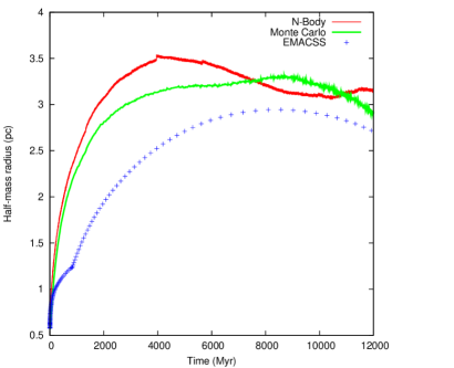
There is no evidence that the presence of anomalous black holes affects the evolution of the half-mass radius, even though they may lead to more vigorous binary formation, hardening and heating. According to “Hénon’s Principle” (Hénon, 1975) the core adjusts so that the rate of heating becomes equal to that required by self-similar evolution of the whole system, and that in turn is determined by global two-body relaxation. (This is what is often referred to as “balanced evolution”.) Thus the rate of expansion of the system need not be determined by the efficiency of the heating mechanism.

3.2 Evolution of the core

Some complications in the evolution of the core have already been hinted at in Sections 2.3.2 and 3.1.2, and are visible in the raw results (Fig.4), as will be discussed. But a further complication is the definition of “core radius”, which is different for the two models. For the $N$-body  model it is based entirely on the density distribution, and is estimated along the lines of Casertano & Hut (1985) as the rms distance from the density centre, weighted by a power of the local density. For the Monte Carlo model the estimate depends on the velocity dispersion and the central density, along the lines of King (1966).

Figure 4: Evolution of core radii for the Monte Carlo and $N$-body  models of M4. Note the effect on the $N$-body  data of the escape of ABH23 and ABH24 at about 4 and 6 Gyr, respectively. Much of the spread in the $N$-body  values is caused by their orbital motion, but other mechanisms contribute noticeably in the first Gyr; see Fig.6.

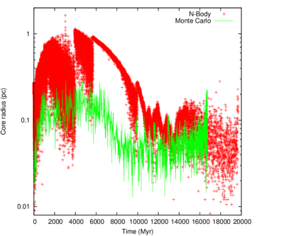
The presence of anomalously massive black holes in the $N$-body  model (Sec.2.3.2) has a dramatic effect on the data. Their motion in the core is responsible for much of the spread in values immediately before the loss of ABH23 just before 4 Gyr. This spread, however, is nothing more than a shortcoming of the definition of the core radius, which is sensitive to the orbital motion of one or more particularly massive bodies. After about 4 Gyr the absence of ABH23 changes the amplitude of the spread, but ABH24 causes a continuing but reduced spread in values until it too escapes at about 6 Gyr. Despite the spread, the upper envelope of the data shows a clear rise up to about 4 Gyr. While it is tempting to hold the anomalous black holes responsible for the rapidity of the rise (as well as for the spread of values, as mentioned above), there is no evidence that the rise would have been any slower with a normal black hole population. Furthermore, despite their continued presence, the rise to about 4 Gyr is followed by a steady fall until about 13 Gyr. These trends match those in the half-mass radius quite well chronologically. Similar remarks (about the trends) may be made about the Monte Carlo model, which suggests that the role of anomalous black holes is at most quantitative.

The end of the decreasing phase in both models is what is referred to in this paper as “(second) core collapse”. After this point there are no such clear trends, but in the Monte Carlo data one can (with care) discern brief, quasi-periodic episodes of small core radius, of which there are about eight between 10 and 14 Gyr. A similar phenomenon was noticed in the Monte Carlo model of the globular cluster NGC 6397 discussed by Giersz & Heggie (2009), and was also visible in an $N$-body  model of that cluster which covered only a short period around an age of 12 Gyr and used initial conditions generated from the evolved Monte Carlo model (Heggie & Giersz, 2009).

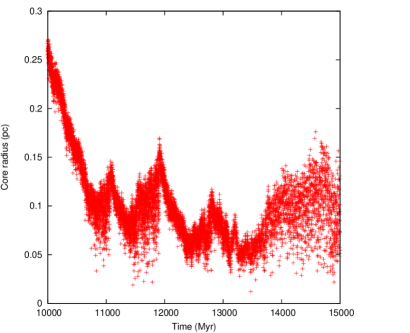
Core evolution in the $N$-body  model after second core collapse is obscured by the Monte Carlo data in Fig.4, and so it is presented alone in Fig.5, which begins just after the escape of ABH25. Second core collapse is quite distinct near 11 Gyr. After about 14 Gyr the spread in values caused by the growth of ABH29 obscures any detail, but between 11 and 14 Gyr there are clear oscillations on a range of timescales and amplitudes. These are not simply caused by the orbital motions of individual black holes, the crossing time of the whole cluster being only 0.99 Myr at 12.5 Gyr, and about 0.02 Myr for the core. Three anomalous black holes (ABH26–28) escape during the evolution shown in Fig.5, but the times of their departure (Table 1) do not seem to be obviously related to any of the features in the plot, and in any case their masses would not be untypical of stellar-mass black holes. The oscillations resemble those observed in the aforementioned $N$-body  model of NGC6397 (Heggie & Giersz, 2009).

Figure 5: Core radius of the $N$-body  model from 10 to 15 Gyr.

The early evolution of the core radius in the $N$-body  model is even more curious (Fig.6). There is a brief contraction, just discernible at the left, until stellar evolution begins at about 5 Myr. The resulting loss of mass causes a rise, but this weakens, and the evolution is reversed by continuing mass segregation. The core, increasingly dominated by black holes, passes through (“first”) core collapse at about 50 Myr, and thereafter exhibits post-collapse expansion. But overlying the expansionary trend is a long sequence of deep oscillations. As with those shown in Fig.5, these cannot be caused by orbital motions of individual black holes, the crossing time at 500 Myr being about 0.04 Myr in the core. The escape of anomalous black holes is also unlikely to be responsible, as most oscillations cannot be associated with these times (Table 1). A plausible explanation of these oscillations is that they are gravothermal.

Figure 6: Core radius of the $N$-body  model up to 1 Gyr.

3.3 Evolution of populations

3.3.1 Binaries

After the rapid erosion of soft binaries near the start, both the $N$-body and Monte Carlo models exhibit rather little evolution of the binary fraction until the end of each model (Fig.7). For most of the evolution the values in the $N$-body  model are in the range 0.047–0.050. In the core the $N$-body  data generally exhibit large fluctuations because of large variations in the estimate of the core radius caused by anomalous black holes (cf. the discussion in the second paragraph of Sec.3.2). Still, it is clear that high values, of order 0.2, prevail at ages in the range 10–12 Gyr. Note that these are binary fractions in the three-dimensional core, not the projected core, in which the binary fraction is 0.046. Similarly, they include all binaries, including binaries with remnant components. If these are excluded, the global binary fraction reduces to 0.035. This is much lower than the range of about 0.10–0.15 reported in a recent study of photometric offset binaries in M4 (Milone et al., 2012). The primordial value is the same as in the Monte Carlo model, and at the time when the latter was developed, the binary fraction was not well constrained (Table 2 in Heggie & Giersz, 2008).

Figure 7: Evolution of the global binary fraction and, for the $N$-body  model, the fraction in the core (dots). For this plot, data was lost around 6 Gyr. Core data is not readily available for the Monte Carlo model.

3.3.2 Degenerate remnants

The numbers of white dwarfs in the $N$-body  and Monte Carlo models are shown in Fig.8. After about 50 Myr the differences merely reflect the different lifetimes and masses of the two models (Sec.3.1.1). Before that the differences are caused by the fact that stellar evolution is not updated as frequently in the Monte Carlo model, because the overall time step is much longer (than in the $N$-body  model).

Figure 8: Numbers of white dwarfs, neutron stars and black holes in the $N$-body  and Monte Carlo models.

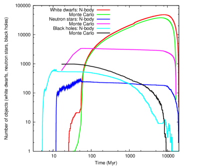
The numbers of neutron stars in the two models, also plotted in Fig.8, are quite different, but only because no natal kicks were applied to neutron stars in the Monte Carlo model. The numbers in the $N$-body  model, where kicks with a 1-dimensional dispersion of 190 km/s were applied, are smaller by a factor of approximately 0.07, which may be taken as an evaluation of the retention factor for this model.

Most problematic is the evolution of the number of black holes (Fig.8 again). Initially the numbers in the Monte Carlo model are higher, because of the absence of natal kicks, though the cadence of the Monte Carlo time steps is hardly adequate at this time. In the $N$-body  model, black holes were formed with natal kicks, except in cases akin to complete “fallback” or “reimplosion” (Woosley & Weaver, 1995), as determined by the recipes of Hurley, Pols, & Tout (2000). The subsequent evolution of the black hole population is greatly affected by the “anomalous” black holes reported in Sec.2.3.2, but it is possible to argue that the numbers are not greatly affected, in the following manner. Breen & Heggie (2013) argued that the rate at which black holes are lost by escape, in particular the rate of mass loss, is determined by the overall evolution of the cluster (mainly, the expansion of the half-mass radius). In the formation of an anomalous black hole a certain number of black holes are removed from the system, but when the “anomalous” black hole eventually escapes, it carries off all the mass of the black holes which contributed to it. The effect, on both the mass and number of black holes, may well be comparable with what would have happened had the evolution of black holes been calculated correctly. At any rate it can be seen that the number of black holes reduces to zero (Monte Carlo) or one ($N$-body) at about the time of second core collapse, a fact which is understandable from the theory of Breen & Heggie (2013); and this time is later in the $N$-body model than in the Monte Carlo model (Sec.3.2).

3.3.3 Collisions, etc

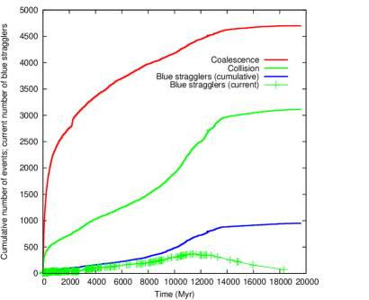
The cumulative number of collisions is plotted in Fig.9, which shows substantial increases around the time of both first and second core collapse. Collisions arise in two-body and higher multiple encounters, and are distinguished from coalescence following Roche-lobe mass transfer. The cumulative numbers of these are also plotted, along with one of the possible outcomes of these events, i.e. the formation of a blue straggler. All three curves flatten out as the model loses almost all its stars towards the end of its life. Note, however, that these are the cumulative numbers formed, and not the current number, which is diminished by escape. As an example, the figure also shows the current number of blue stragglers (defined as main sequence stars with a mass at least 1.02 times the turnoff mass).

Figure 9: Numbers of collisions, coalescences, and events leading to the formation of blue stragglers; and the current number of blue stragglers. The last of these is based on much more sparsely sampled data.

4 Comparison with observations

4.1 Surface brightness profile

For the purposes of comparison with observations, the state of the model was extracted from the complete dump file at a simulated time of 12 Gyr, which is the age for M4 that has been assumed in this study, as in Heggie & Giersz (2008). To compute the surface brightness, the positions were first projected along the three coordinate axes, and the location of the centre of the cluster was taken to lie at the median values of the coordinates. The surface brightness was computed in a series of annuli, uniform in the logarithm of the projected radius, and averaged over the three projections. Since the dump file includes only the luminosity and radius of each star, a simple bolometric correction was applied (Reed, 1998), but it was also verified that $V$-magnitudes, calculated according to recipes kindly provided by J. Hurley, produced an almost indistinguishable surface brightness profile. Extinction was applied to the resulting surface brightness, and the result is compared with the observational profile from Trager et al. (1995) in Fig.10.

Figure 10: Surface brightness of the model at 12 Gyr, compared with the observational profile of Trager et al. (1995). The size of points in the latter is determined by the weight which those authors assigned to different data; note in particular the scatter of small points at small radii. The model profile at 11.9 Gyr is also shown.

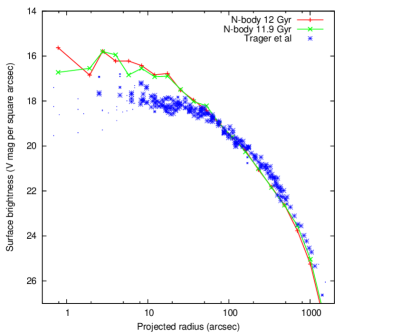
While the overall size of the model is acceptable, in detail the profile is too concentrated. The central surface brightness is too bright by about two magnitudes, and the profile is too dim beyond about 100 arcsec, i.e. not far outside the observational core radius of about 70 arcsec (Harris, 1996, 2010 revision). In almost every respect the Monte Carlo model did better (Fig.1 in Heggie & Giersz, 2008). The Monte Carlo code (now called MOCCA) has been improved considerably since the time of that study (Giersz et al., 2013), and it is possible that the newer version would share the problems of the $N$-body  model, indicating merely that the initial conditions were not optimal for either the $N$-body  code or MOCCA. But the problem does not appear to lie with the model at 12 Gyr. Though the dynamical core radius appeared to be somewhat larger at 11.9 Gyr (Fig.4), suggesting that the $N$-body  model would appear less concentrated, the surface brightness profile was little better (Fig.10).

A possible reason for the brighter, smaller core in the $N$-body  model is the relative paucity of black holes and neutron stars. It is known (Merritt et al., 2004; Mackey et al., 2008) that a large retained population of black holes drives an expansion of the core radius, and it may be that a large retained population of neutron stars could enhance this effect slightly. Incidentally, the central mass to light ratio (in projection) is $M/L_{V}\simeq 1.4$ in solar units, while the global value is 2.16.

4.2 Velocity dispersion profile

To construct the velocity dispersion profile (Fig.11), an average over three lines of sight (i.e. the three coordinate axes) is again taken, and only stars brighter than a limit about 2 magnitudes fainter than turnoff have been used. For each projection the stars were binned in projected radius centred on the density centre, the mean square line-of-sight velocity was corrected for the mean l.o.s. velocity of the cluster, and the results were averaged over the three projections.

Figure 11: Line-of-site velocity dispersion in the $N$-body  model, compared with the observational data of Peterson et al. (1995).

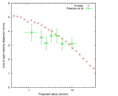
The agreement with observational data (Peterson et al., 1995) is certainly no worse than for the surface brightness profile. The observational data is confined to the region from about the core radius outward, and again the problems of the $N$-body  model seem mainly confined to the region of the core, much as in Fig.10. At $69300M_{\odot}$, the $N$-body  model is somewhat more massive than the Monte Carlo model ($46100M_{\odot}$) at age 12 Gyr (Fig.2), which itself provided a satisfactory fit to the observational data, and this is sufficient quantitatively to account for the poorer results in Fig.11. The fact that the $N$-body  model, with a half-mass radius of 3.13 pc, is slightly larger than the Monte Carlo model (2.90 pc) makes little difference.

4.3 Luminosity functions

Here the $N$-body  model will be compared with the innermost and outermost of the four local luminosity functions observed by Richer et al. (2004). Again the model results have been obtained by projecting the model along the three coordinate axes. In the model, those stars were counted which lay in two annuli which have the same area and median radius (after dimensional scaling) as in the two observational fields. The results are compared in Fig.12.

Figure 12: V luminosity functions in annuli with median radii of 0.938 (top) and 5.028 arcmin (bottom). The $N$-body  model is compared with the observational data of Richer et al. (2004) and the Monte Carlo results of Heggie & Giersz (2008).

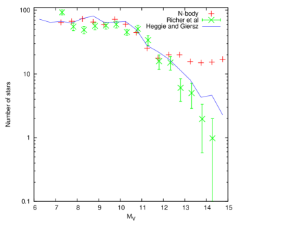
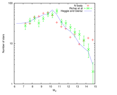
Since both the observational and $N$-body  data are numbers of stars in a given area, the Poisson errors will be comparable, even though error bars are only given for the observational data. The most noticeable feature of the inner profile (top) is the great excess of stars at the faintest magnitudes. Part of this may perhaps be attributed to completeness, for which the observational data were not corrected. According to Richer et al. (2002), incompleteness in the outer field is negligible down to $M_{V}=15$, though it could presumably be significant in the inner field. Another possible explanation is the effect of anomalous black holes, as Gill et al. (2008) found that mass segregation was diminished in $N$-body models by the presence of an intermediate-mass black hole. But in their models the smallest black hole mass was 0.9% of the cluster mass, while for the most massive anomalous black hole in the $N$-body  model of M4 (at least, at any time since the escape of ABH24 almost 7 Gyr earlier) the fraction is about 0.1%, which diminishes the strength of this mechanism. Whatever the explanation, the $N$-body  data greatly exceeds the corresponding result for the Monte Carlo model at faint magnitudes in the inner field (Fig.12, top), indicating once again considerable differences between the two models. Nevertheless in the outer field (Fig.12, bottom) the comparison with the observational data is not very discrepant, except at the faintest magnitudes, and near the peak of the observational luminosity function: the reduced chi-square is 2.2, of which about half is contributed by the points at magnitudes 10.75 and 14.75.

5 Conclusions and discussion

5.1 Conclusions

In this paper results are reported of the largest sustained $N$-body  model of a globular star cluster to date. It began with $N=484710$ stars, and took about two years and eight months, using the code NBODY6 with extensions for GPU support (Nitadori & Aarseth, 2012). The initial conditions were generated from a Monte Carlo model (Heggie & Giersz, 2008) which, after 12 Gyr of simulated evolution, resembled the globular star cluster M4 in respect of its surface brightness and radial (line-of-sight) velocity dispersion profiles, and its observed luminosity function at two radii.

The evolution of the total mass and half-mass radius in the $N$-body  and Monte Carlo models are fairly comparable (Figs.2, 3), though the mass of the Monte Carlo model is systematically smaller, leading to a shorter-lived model. This may be caused by the treatment of escape in the Monte Carlo model. The larger mass of the $N$-body  model is one factor which may contribute to the moderate disagreement, at small projected radii, between the line-of-sight velocity dispersion of the model and the observational data (Fig.11). The evidence of the luminosity function, when compared with observational results (Fig.12), is that some excess mass may be found in the lower main sequence at small projected radii. The most serious disagreement, however, concerns the surface brightness profile of the core, where the $N$-body  model is too bright to be consistent with observations (Fig.10). The most plausible explanation for this is the relatively small retention factor of black holes and neutron stars, at least by comparison with the Monte Carlo model (Fig.8), where no natal kicks were applied.

Discussion of the core radius is complicated by a recurrent error in the $N$-body  model, which led to spurious coalescence of degenerate remnants, especially black holes (Table 1). Though it can be argued that this does not affect the bulk evolution, its effect on the core cannot be so readily dismissed. One of these effects is the resulting size of fluctuations in the estimated core radius when these “anomalous” massive black holes were present (Fig.4). Nevertheless these anomalous black holes do not seem to be responsible for some very interesting aspects of core evolution, especially the oscillations observed in the core radius in about the first Gyr of the simulation, and even at times around the present age of M4 (Figs 5,6).

There is rather little evolution of the binary fraction, except in the core (Fig.7), though the value is too low for consistency with observational data, because of a poor choice of the initial value. Though this initial binary fraction was 7%, almost 5000 of the binaries led to coalescence as a result of Roche-lobe overflow (Fig.9), which is considerably more than the number of stellar collisions in encounters. About a thousand of all these events were identified by the code as leading to the formation of a blue straggler.

5.2 Discussion

Evidently the $N$-body  model presented in this paper fails to serve as a completely satisfactory model of M4. Faults could lie within aspects of the dynamical evolution of M4 which are excluded in the $N$-body  and Monte Carlo models, such as the formation of a second generation, or conceivably the rotation of the cluster. The choice of a circular Galactic orbit in a point-mass Galactic potential was made to facilitate comparison with the Monte Carlo results, and implicitly ignores the effects of disk and bulge shocking. Actually, no greater effort would have been required to use a more realistic orbit (see, for example, Dinescu, Girard, & van Altena 1999) and potential. But within the self-imposed constraints of the modelling underlying this paper, it is worth considering how a better model might be found, besides some obvious improvements in the initial conditions, such as the primordial binary fraction.

Some technical problems of the $N$-body  model are easily avoided, such as occurrence of the spurious collisions between black holes which marred the model described in this paper. But it is clear that there is one important respect in which the $N$-body  model was physically more realistic than the Monte Carlo model which generated the initial conditions, and that is the treatment of natal kicks given to black holes. The first step to be taken, then, could be to repeat the Monte Carlo calculation, but using a similar prescription for natal kicks as in the $N$-body  model. If it turned out that such a Monte Carlo model exhibited a similar bright core to that of the $N$-body  model, it would add significant confirmation of the reliability of the Monte Carlo model for this kind of work. Then it would be profitable to repeat the exercise of using the Monte Carlo model to find appropriate initial conditions for M4, especially as the Monte Carlo code (now named MOCCA) has been improved substantially in the meantime. Likewise, ongoing improvements in $N$-body  modelling might then make it possible to confirm the new Monte Carlo results with $N$-body  techniques in less time than was taken for the $N$-body  model described in this paper.

An important point exposed by this discussion is the role played by the fit to the surface brightness profile. If the comparison (between the models and with the cluster) had been restricted to a discussion of the half-mass radius and the mass then it would have been much less clear how unsatisfactory the $N$-body  model was. A second important point is the continuing central role played by the Monte Carlo method in this field. Finding initial conditions requires the computation of many models – at least a few dozen. Even if the run-time of an $N$-body  model could be reduced from two or three years to two or three months, the time required for finding appropriate initial conditions for a single cluster would still be many years.

References

- Aarseth (1999) Aarseth S. J., 1999, PASP, 111, 1333
- Aarseth (2003) Aarseth S. J., 2003, Gravitational N-Body Simulations. Cambridge University Press, Cambridge
- Alexander et al. (2014) Alexander P. E. R., Gieles M., Lamers H. J. G. L. M., Baumgardt H., 2014, MNRAS, 442, 1265
- Bedin et al. (2013) Bedin L. R., et al., 2013, AN, 334, 1062
- Breen & Heggie (2013) Breen P. G., Heggie D. C., 2013, MNRAS, 432, 2779
- Casertano & Hut (1985) Casertano S., Hut P., 1985, ApJ, 298, 80
- Dinescu, Girard, & van Altena (1999) Dinescu D. I., Girard T. M., van Altena W. F., 1999, AJ, 117, 1792
- Fregeau & Rasio (2007) Fregeau J. M., Rasio F. A., 2007, ApJ, 658, 1047
- Giersz (1998) Giersz M., 1998, MNRAS, 298, 1239
- Giersz & Heggie (2009) Giersz M., Heggie D. C., 2009, MNRAS, 395, 1173
- Giersz & Heggie (2011) Giersz M., Heggie D. C., 2011, MNRAS, 410, 2698
- Giersz, Heggie, & Hurley (2008) Giersz M., Heggie D. C., Hurley J. R., 2008, MNRAS, 388, 429
- Giersz et al. (2013) Giersz M., Heggie D. C., Hurley J. R., Hypki A., 2013, MNRAS, 431, 2184
- Gill et al. (2008) Gill M., Trenti M., Miller M. C., van der Marel R., Hamilton D., Stiavelli M., 2008, ApJ, 686, 303
- Harris (1996) Harris, W. E. 1996, AJ, 112, 1487
- Hasani Zonoozi et al. (2014) Hasani Zonoozi A., Haghi H., Küpper A. H. W., Baumgardt H., Frank M. J., Kroupa P., 2014, MNRAS, 440, 3172
- Hasani Zonoozi et al. (2011) Hasani Zonoozi A., Küpper A. H. W., Baumgardt H., Haghi H., Kroupa P., Hilker M., 2011, MNRAS, 411, 1989
- Heggie & Giersz (2008) Heggie D. C., Giersz M., 2008, MNRAS, 389, 1858
- Heggie & Giersz (2009) Heggie D. C., Giersz M., 2009, MNRAS, 397, L46
- Heggie & Giersz (2014) Heggie D. C., Giersz M., 2014, MNRAS, 439, 2459
- Hénon (1971) Hénon M. H., 1971, Ap&SS, 14, 151
- Hénon (1975) Hénon M., 1975, IAUS, 69, 133
- Hurley, Pols, & Tout (2000) Hurley J. R., Pols O. R., Tout C. A., 2000, MNRAS, 315, 543
- Hurley, Tout, & Pols (2002) Hurley J. R., Tout C. A., Pols O. R., 2002, MNRAS, 329, 897
- Joshi, Rasio, & Portegies Zwart (2000) Joshi K. J., Rasio F. A., Portegies Zwart S., 2000, ApJ, 540, 969
- King (1966) King I. R., 1966, AJ, 71, 64
- Kroupa (1995) Kroupa, P. 1995, MNRAS, 277, 1507
- Kroupa, Gilmore, & Tout (1991) Kroupa P., Gilmore G., Tout C. A., 1991, MNRAS, 251, 293
- Mackey et al. (2008) Mackey A. D., Wilkinson M. I., Davies M. B., Gilmore G. F., 2008, MNRAS, 386, 65
- McLaughlin & van der Marel (2005) McLaughlin D. E., van der Marel R. P., 2005, ApJS, 161, 304
- Merritt et al. (2004) Merritt D., Piatek S., Portegies Zwart S., Hemsendorf M., 2004, ApJ, 608, L25
- Milone et al. (2012) Milone A. P., et al., 2012, A&A, 540, A16
- Nitadori & Aarseth (2012) Nitadori K., Aarseth S. J., 2012, MNRAS, 424, 545
- Peterson et al. (1995) Peterson, R. C., Rees, R. F., & Cudworth, K. M. 1995, ApJ, 443, 124
- Reed (1998) Reed B. C., 1998, JRASC, 92, 36
- Richer et al. (2002) Richer H. B., et al., 2002, ApJ, 574, L151
- Richer et al. (2004) Richer, H. B., et al. 2004, AJ, 127, 2771
- Sippel & Hurley (2013) Sippel A. C., Hurley J. R., 2013, MNRAS, 430, L30
- Trager et al. (1995) Trager, S. C., King, I. R., & Djorgovski, S. 1995, AJ, 109, 218
- Woosley & Weaver (1995) Woosley S. E., Weaver T. A., 1995, ApJS, 101, 181