Foucault’s method in new settings

Abstract

In this paper, we introduce two simple and inexpensive versions of the well-known Foucault method for measuring the speed of light. In a footprint of just 20 cm by 270 cm with readily available laboratory items and a webcam, we obtained $c=296720\pm 3000$ km/s, and $c=302295\pm 3000$ km/s, respectively, both within less than a per cent of the defined value. The experiment also prepares students to work with large amounts of data.

I Introduction

In recent years, we could witness a substantial paradigm shift in sciences: relationships emerge from vast amounts of collected data (sometimes dubbed big data), and not just a few measurements. Notable examples are customer recommendation systems of Amazon, eBay and similar retailers, or the data streams of the Large Hadron Collider or the Square Kilometre Array. This trend is expected to continue in the foreseeable future, especially, with the advent of always-online mobile devices capable of continuously collecting and transmitting all kinds of data.

However, it also seems that science education does not keep up with the pace of progress in data collection and analysis capabilities, and that many introductory or even advanced level laboratory experiments are still conducted with hand-held stopwatches, weights, mercury thermometers, and microscopes with engraved scales. This approach has at least three inherent problems. The first is that it teaches students how experiments were conducted two centuries ago, but does not tell them how to do them now. Second, the amount of data that can be collected in this way is limited, and inaccurate. This also means that statistical evaluation of the results is constrained to a handful of data points. Finally, by the very nature of the required specialized setups, these experiments are expensive, and students have to operate within the spatial and temporal confines of the laboratory course. We are convinced that one cannot underestimate the pedagogical benefits of pursuing science on the kitchen sink: when one can accurately measure something relevant (such as, a fundamental constant) with easily available and cheap everyday items, and without reference to a dedicated laboratory. It is a very fortunate coincidence that in our times, everyday items are digital gadgets capable of measuring all kinds of physical quantities, e.g., distance, temperature, acceleration, magnetic fields, light intensity, frequency, time etc., and that the demand for high quality in user experience makes it possible to deliver unprecedented accuracy.

At the same time, we also recognize the pedagogical value of discussing how experiments were conducted in the past and that it would be an irreparable loss not to show what could be achieved with devices that we would now consider rudimentary. What we would like to demonstrate in this paper is that it is not necessary to regard the above-mentioned two subjects, historical perspective, and progress in measurement capabilities as disjoint. There are ways of showing the beauty and ingenuity of past experiments, while reaping the many benefits of modern technologies in terms of measurement time, accuracy, cost, or the volume of data.

The example that we take is the measurement of the speed of light, which is one of the fundamental physical constants. Strictly speaking, our example is pathological in the sense that the international meter is defined by the help of the speed of light and the international standard of time, and not the other way around. However, first, till 1983 (i.e., in Foucault’s life), length and time were defined and the speed of light was the derived quantity, second, this fact does not reduce the didactic value of the experiment itself. We would like to emphasize that while the evaluation of the measurements requires some data processing, this fact does definitely not qualify it as a big data exercise.

The paper is organized as follows. In the next two sections, we outline the historical and theoretical background and derive the expression for $c$. In Section IV., we introduce our experimental setup and the critical components, Section V. contains a detailed discussion of our results, while Section VI. is devoted to a thorough analysis of various systematic errors. In the appendix, we present a couple of MATLAB (The Mathworks, Inc.) snippets that can be used to evaluate measurement data.

II Historical background

That the speed of light, $c$, is finite was already conjectured by Galileo in the XVII. century, though, his experimental apparatus at the time prevented him from giving even an order-of-magnitude estimate for the value. Since then, various methods have been developed.

It was first Huygens, who, based on the astronomical measurements of Rømer in 1676 on the entry into and exit from eclipses of Jupiter’s moons, could provide a lower bound of about 200 000 km/s. The same measurements, repeated with higher accuracy by Delambre in 1809, yielded 304 000 km/s, astonishingly close to the true value. Another astronomical method, the aberration of light, was discovered by Bradley in 1729, with the result of about 296 000 km/s.

Later, it was realized that in Maxwell’s theory, the speed of light is linked to fundamental electromagnetic constants through the relation $\epsilon_{0}\mu_{0}=c^{-2}$, and therefore, by measuring the vacuum permittivity $\epsilon_{0}$, and the vacuum permeability $\mu_{0}$, it is possible to indirectly infer the value of $c$ Clark (1956, 2001).

It is also to be noted that, if the frequency $f$ of electromagnetic radiation is known, and the wavelength $\lambda$ can be measured, then by dint of the relation $c=f\lambda$, $c$ can be indirectly determined. This is the basis of measurements of interferometric methods Belich et al. (1996); Lahaye et al. (2012), and of cavity resonance methods D’Orazio et al. (2010).

Finally, there are several methods that measure the time of flight in terrestrial settings. One of them is the Foucault method that we discuss in more detail in the next section Dillman (1964); Feagin (1979); Morrison and Driedger (1980); Brody et al. (2010), while with the advent of high-speed electronics, it is now possible to directly measure the delay in the arrival of short optical pulses as the distance between the emitter and receiver is increased Rogers et al. (1969); Deblaquiere et al. (1991); Aoki and Mitsui (2008); Ronzani et al. (2008). This latter method is the simplest of all, but it definitely lacks the elegance of the others.

The interested reader can find a more detailed survey of various measurement methods and their significance in Bates (1988).

III Theoretical background

Foucault’s is one of the simplest methods of measuring the speed of light on Earth, and it falls into the category of time of flight measurements. It is based on the observation that, if a light beam bounces off a moving mirror twice, the mirror will have moved by a small amount by the time it is hit by the beam the second time, and this movement results in a small displacement of the reflected beam. It is this displacement that is to be measured, and from where the speed of light is to be inferred. In this particular instance, the mirror is rotating, and the rotation angle between the two events can simply be related to the time that was required for the round trip. The speed of light can be obtained from the measured displacement, and the length of the round-trip path. Due to its conceptual simplicity, this is perhaps the most popular method in student laboratories.

To be more specific, let us take the simplified experimental setup shown in Fig. 1. A point source emitting light is located at point $S$, at a distance $d_{1}$ from the lens $L$. The source’s light is reflected by the rotating mirror $RM$ (at a distance of $d_{2}$ from the lens, and at this point, stationary) and its image is created at the position of the end mirror $M$, which is at a distance of $d{}_{3}$ from the rotating mirror, and is normal to the in-coming light. This also means that the light reflected by $M$ is focused on $S$ again. In the absence of the rotating mirror, the image of $S$ would be at $V$.

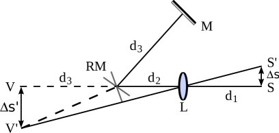
Figure 1: The concept of the experiment. $RM$ is the rotating mirror, $M$ is the end reflector, and $L$ is a lens. $S,S^{\prime}$ are the light source, and its image, respectively, while $V$, and $V^{\prime}$ are the virtual images of $S$, and $S^{\prime}$.

Now, let us assume that in the time $\Delta t$ the light traverses the distance between $RM$ and $M$ in both directions, the rotating mirror turns by an amount $\omega\Delta t$, where $\omega$ is the angular velocity, and $\Delta t=2d_{3}/c$. This rotation displaces the virtual image $V$ to $V^{\prime}$, where the distance between these two points is simply $\Delta s^{\prime}=2\omega\Delta t\cdot d{}_{3}$. The factor of $2$ is a result of the reflection on $RM$: upon reflection, all angles change by a factor of $2$. The image of the virtual point $V^{\prime}$ is mapped by the lens to the point $S^{\prime}$, and using the two similar triangles formed by $V,V^{\prime}$, and the lens, and $S,S^{\prime}$, and the lens, respectively, we conclude that the distance between $S$ and $S^{\prime}$ is

$$\Delta s=\frac{d_{1}}{d_{2}+d_{3}}\Delta s^{\prime}=2\omega\Delta t\frac{d_{1}d_{3}}{d_{2}+d_{3}}=\frac{4d_{1}d_{3}^{2}}{d_{2}+d_{3}}\frac{\omega}{c}\ ,$$

i.e., the speed of light is

$$c=\frac{4d_{1}d_{3}^{2}}{d_{2}+d_{3}}\frac{\omega}{\Delta s}\ .$$ (1)

Given $d_{1,2,3}$, the speed of light can be gotten by measuring the displacement $\Delta s$ for a given angular speed. In principle, to determine $c$, a single measurement point is enough, but as we will see later, by measuring $\Delta s$ as a function of $\omega$, and taking the slope of the linear dependence, it is not necessary to find the reference position at $\omega=0$. Re-arranging Eq.(1) yields

$$c_{0}=\frac{4d_{1}d_{3}^{2}}{d_{2}+d_{3}}\left(\frac{d\Delta s}{d\omega}\right)^{-1}\ .$$ (2)

In Section VI., we will show that the errors are negligible, if the lens is not positioned perfectly, and the image of $S$ is not formed at $M$. In the formula above, $c_{0}$ indicates that these errors are not yet taken into account.

IV Experimental setup

Fig. 2 displays our first experimental setup. Laser light from a standard fibre fault locator (OZ Optics, FODL-43S-635-1) emitting at a wavelength of 635 nm is transmitted through a single-mode fibre, and collimated by a short focal length fibre collimator (Thorlabs F240FC-B). While it is not absolutely necessary, by passing the light through the single-mode fibre patch cable (Thorlabs P1-630A-FC-1), we begin with a perfect Gaussian beam. It is worth noting that the fault locator can be replaced by an inexpensive laser pointer.

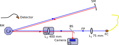
Figure 2: Experimental setup Setup 1. $RM$, $FM$, $SM$ are the rotating, folding, and back reflector mirrors, respectively, $L_{1}$, $L_{2}$ are lenses of focal length 75 and 400 mm, respectively, $FP$ is the focal point of $L_{1}$, $FC$ is the fibre collimator, $BS$ is the beamsplitter, and $TS$ are translation stages. Dimensions are given in the text.

The collimated beam is then lead through a telescope consisting of two lenses of focal lengths 75 mm ($L_{1}$), and 400 mm ($L_{2}$), respectively. The telescope is misaligned slightly in the longitudinal direction (the distance between the two lenses is larger than 475 mm), so that the beam leaving is not collimated any more, but, after being reflected on the rotating mirror $RM$, is focused on a spherical mirror $SM$, which acts as the back reflector. The rotating mirror is located at a distance of 1630 mm from the 400-mm lens, while the back reflector with a radius of curvature of 4000 mm is positioned at a distance of 4830 mm from the rotating mirror. Distances were measured with a tape measure. In order to reduce the overall size of the setup, the 4830-mm path was folded by the insertion of a flat mirror (not shown) between $RM$, and $SM$, $FM$. We should also note that since the spherical mirror is not involved in the imaging, it can be replaced by a flat mirror.

For monitoring the rotation, we also placed a standard silicon photodiode (Thorlabls PD136A) close to the rotating mirror: when rotating, the mirror diverts the laser light to the diode 8 times per revolution, thereby, producing a well-defined potential spike that can conveniently be recorded on an oscilloscope.

The light reflected by the spherical mirror travels along the same path, except that it is diverted to a webcam (Logitech C310) by a pellicle beam splitter ($BS$, Thorlabs BP150) positioned to the left of $FP$, which is the focal point of $L_{1}$. The small lens of the webcam has to be removed before use, so that no extra imaging element is introduced. In the original version of the experiment, instead of a camera, a microscope is used to measure the displacement of the beam. However, given the finite size of the focal spot, this also entails that large distances have to be employed in order to realize measurable displacements. The application of the camera not only makes data collection more convenient, but it also implies that the physical size of the setup can considerably be reduced. We would like to point out that the use of a webcam in the context of speed of light measurements was discussed in an interferometric setting in Lahaye et al. (2012).

Our second setup, Setup 2, is shown in Fig. 3. The light of the fault locator is focused by a lens of focal length $400\,\mathrm{mm}$ onto $FP$, from where it reaches the spherical mirror $SM$ with a focal length of 2 m. The spherical mirror is $4060\,\mathrm{mm}$ away from $FP$, and is tilted slightly, so that the light is reflected off the rotating mirror $RM$, located $730\,\mathrm{mm}$ away from $SM$, and finally $FM$, located $3260\,\mathrm{mm}$ away from $RM$. The lengths in the setup are chosen in such a way that the light is focused on the flat end reflector, $FM$, although, as will be discussed in Section VI., small longitudinal misalignments do not influence the results in any significant way. As in the first setup, folding mirrors were used between $SM$, and $RM$, and between $RM$, and $FM$.

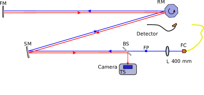
Figure 3: Experimental setup, Setup 2. $RM$, $FM$, and $SM$ are the rotating, flat, and spherical mirrors, respectively, $L$ is a lens of focal length 400 mm, $FC$ is the fibre collimator, $BS$ is the beamsplitter, and $TS$ are translation stages. Dimensions as indicated in the text.

The two setups are conceptually the same: the only difference between them is that the imaging element in the first case is a lens, while in the other case, it is a spherical mirror.

As the rotating reflector, we employed an octagonal printer mirror scavenged from a faulty printer, shown in Fig. 4. (This part can also be purchased separately. A possible alternative is a barcode reader with a revolving mirror.) Laser printers utilize a focused laser beam to locally discharge a positively pre-charged cylindrical drum, that is itself rotating around its own axis. The octagonal (sometimes quadratic, or hexagonal) mirror is used for scanning the laser beam along the axis of the drum, thereby creating an accurate time-to-two-dimensional mapping on the drum’s surface. In order to achieve high spatial accuracy, both the drum and the rotating mirror have to revolve at a constant speed. Stabilization of the rotation frequency is achieved by means of phase-locked loops (PLL), in which an external clock signal is locked to the signal of a magnetic field transducer measuring the temporal variations of the field of a constant magnet moving with the axle of the motor. This also means that, within limits, the rotation speed can be set by adjusting the clock signal that is fed into the PLL loop. Fig. 4 also indicates the connections of the mirror assembly: $PWR$ (pin 1) is the power line, whose potential can be anything between +18, and +36 V, $GND$ (pin 2) is ground, $ENAB$ (pin 3) is the active-low motor enable pin (this should be tied to ground), while $CLK$ (pin 5) is the clock line, which takes TTL pulses with frequencies between around 300, and 6000 Hz. Pin 4 is an output connected to the magnetic field transducer, and can be used for monitoring the rotation.

The advantages of the mirror assembly are that first, the mirror is monolithic, therefore, it is safe to operate: no pieces can break off at high speeds. Second, the control electronics makes it possible to adjust the speed by setting the frequency of the clock signal from a simple function generator, and that there is a well-defined linear relationship between the rotation speed and the clock frequency.

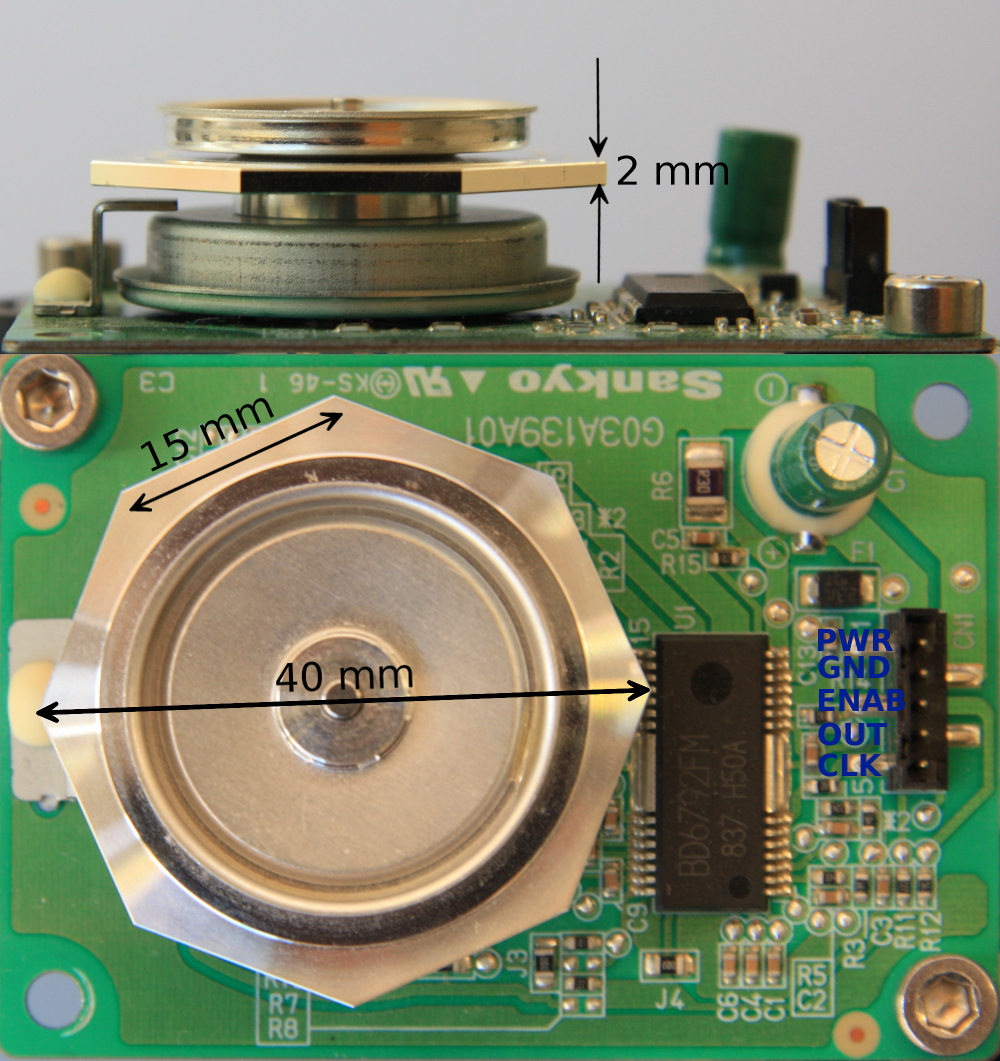
Figure 4: Rotating printer mirror, side view (top), and top view (bottom). The 30-pin integrated circuit contains the motor driver (BD6792FM from Rohm Semiconductors) with the built-in PLL. Control pins are labeled in blue.

Initial alignment of the setup is performed when the mirror is stopped (the enable line is high). First, all mirrors are placed to their respective positions, and $FC$ is aligned such that the collimated laser beam can travel to the end mirror, $SM$. Then $L_{1}$ is inserted in such a way that the diverging laser light still reaches both $RM$, and $SM$. After this, $L_{2}$ is inserted in the path, and is moved along the optical axis till the size of the light spot reaches its minimum on $SM$. When this is achieved, the beamsplitter, $BS$, has to be placed on the left hand side of the focal point of $L_{1}$, at a distance of about 5-7 cm from the focal spot, $FP$. With the tip-tilt control knobs of the mirror holder, $SM$ has now to be aligned so that the light is reflected back to the laser. At this point, the reflected beam should be focused on $FP$. Finally, the camera has to be placed in the diverted focus of the back-reflected beam. Great care has to be taken to make sure that the camera’s plane is as perpendicular to the laser beam as possible: failure to do so will results in a systematic error, which leads to higher speeds of light. For a thorough discussion on this, see Section VI.

V Experimental results

As can be inferred from Eq.(2), in order to determine the speed of light, one has to measure $d_{1,2,3}$, the angular frequency $\omega$, and the displacement $\Delta s$. The measurement can be done in the same way in both setups, and the steps are as follows. First, one has to determine the rotation speed as a function of the clock frequency. Next, the pixel size of the camera has to be measured. This step amounts to calibrating a ruler. Then the displacement of the image on the camera has to be measured at various clock frequencies (this step involves fitting to the camera images), and by using the pixel size, this displacement has to be converted to physical units. Finally, the slope of the displacement-frequency relationship has to be determined, and inserted in Eq.(2).

The rotation speed can be deduced from the time traces of the photodiode, either by simply measuring the time difference between an integer number of maxima, or recording the potential values, taking the Fourier transform, and identifying the strongest frequency component. Given a high enough number of samples, the two methods deliver the same results. In Fig. 5, we show the measured rotation speed as a function of the clock frequency, with a typical time trace of the detector signal on an oscilloscope, and its Fourier transform. The period can clearly be resolved from either the signal, or its Fourier spectrum. Note that at high clock rates, the rotation speed saturates. For this reason, we excluded the last 3 points from the linear fit, from which we deduced the relationship $f_{\mathrm{rot}}(Hz)=(0.167\pm 0.00054)\cdot f_{\mathrm{clk}}(\mathrm{Hz)}-0.649\,\mathrm{(Hz)}$. The error of the fit is approximately 0.3%. Given the precision (in the ppm range) of frequency standards used in modern pulse generators, and the stability of phase-locked loops used in laser printers, we ascribe the error to our way of determining the frequency from the Fourier transform of the time trace. Also note that, since the rotating mirror has 8 facets, the actual rotation speed is only 1/8 of what the detector signal indicates.

It is worth pointing out that, given the order of magnitude of the rotation speed, in the absence of an oscilloscope, these frequencies can easily be measured by means of a smart phone. All one has to do is to convert the electrical signal of the photodiode to sound by amplifying it, and connecting it to a speaker, and then record the sound through the microphone. There are countless applications that can take and display the Fourier transform of the microphone input. Likewise, the clock signal can be generated by a suitable waveform applied to the phone’s speaker.

Figure 5: Rotation speed as a function of clock frequency. The inset in the lower right corner shows a typical time trace on the detector with its Fourier spectrum in the upper left. The clock frequency for this trace is 300 Hz. The parameters of a linear fit are displayed in the figure. The last three data points (blue squares) were excluded. The error in the slope is 0.00054.

In order to convert the pixel positions into physical distance, we have to calibrate the CCD camera. In other words, we have to measure the pixel size. For this procedure, we stopped the rotating mirror, and shifted the camera by an amount indicated by the micrometer screw on the translation stage. The data points are plotted in Fig. 6 in conjunction with a linear fit, which gives a pixel size of $2.75\,\mu\mathrm{m}$. This is also the value given by the manufacturer. By the help of this measurement, one can also ascertain that the translation axis is parallel to the camera’s plane, because if that is not the case, then the width of the profiles changes as the camera is shifted. As shown below (see e.g., Fig. 8), the centre of the nearly Gaussian profiles can be obtained with sub-pixel accuracy. If we take half of the smallest micrometer division ($10\,\mu\mathrm{m}$) as the error in position, this procedure incurs an overall error of less than one fifth of a per cent.

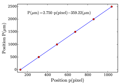
Figure 6: Measurement of the pixel size. The statistical errors in both the dependent and independent variables are too small to be visible. The parameters of the linear fit are indicated in the figure.

Having determined the calibration for both the camera, and the rotation speeds, we now turn to the measurement of the displacements. First we discuss the results obtained from Setup 1. Typical images of the reflected beam at three different rotation speeds (183, 417, and 885 Hz) are shown in Fig. 7 (only a small part of the otherwise 720-by-1280 chip is displayed). The movement of the beam is clearly visible. Note that, while we begin with a circularly symmetric Gaussian beam (this is what leaves the single-mode fiber), the camera image is elongated along the vertical direction, which is perpendicular to the direction of the displacement. The reason for this is that the mirrors are only 2 mm thick, but 15 mm wide, while the beam at the mirror’s position is still about 10 mm in diameter. This means that diffraction will stretch the beam in the direction of the smallest dimension of the mirror.

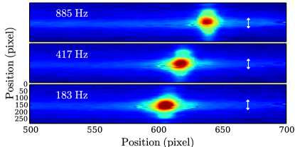
Figure 7: Typical camera images in Setup 1 at rotation frequencies 183, 417, and 885 Hz, respectively. The profiles below were obtained by integrating over the region indicated on the right hand side by the small white arrows.

The images in Fig. 7 are turned into nearly Gaussian profiles by vertically integrating over a range of $\pm 25$ pixels around the maximum, as indicated by the small white arrows in the figure. Such profiles for three different rotation speeds (183, 417, and 885 Hz) are shown in Fig. 8. In order to accurately determine the centre positions of these profiles, we fit a Gaussian with an offset to the data points in a range of $\pm 15$ pixels around the pixel with the highest intensity, as shown by the shaded gray domains in the figure. The centre of these fits is then accepted as the true position of the reflected beam. The error in the fit is less than $0.15$ pixels for all measurements.

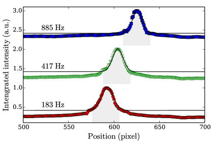
Figure 8: Typical profiles taken in Setup 1 at a rotation frequency of 183 (solid red circle), 417 (empty green triangle), and 885 Hz (solid blue square), respectively. The domain of Gaussian fits is indicated by the shaded gray regions, while the solid black lines are the fits.

Figure 9 contains measurement data on the beam displacement as a function of the rotation speed. On the right vertical axis, the positions are given in terms of the CCD pixels, as taken from images similar to Fig. 7. The left axis displays the positions in physical units, after the CCD pixels were converted using the fit from Fig. 6. The linear fit to these data yields a slope of $(0.130\pm 0.00047)\,\mathrm{\mu m/Hz}$. Given that, with the nomenclature of Eq. (2), $d_{1}=425\pm 1\,\mathrm{mm}$, $d_{2}=1630\pm 1\,\mathrm{mm}$, and $d_{3}=4830\pm 1\,\mathrm{mm}$, and taking all above-mentioned error sources into account, we calculate a speed of light of $c=(2.97\pm 0.03)\cdot 10^{8}\,\mathrm{m/s}$. This is within 1% of the defined value of $2.99792458\cdot 10^{8}\,\mathrm{m/s}$, and overall, the statistical errors are within 1%.

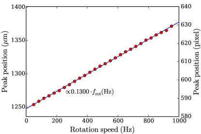
Figure 9: Position of the reflected beam as a function of the rotation speed in Setup 1. On the right vertical axis, the same data are shown in units of the CCD pixels. The peak position can be obtained from $P_{\mathrm{peak}}(\mathrm{\mu m})=(0.130\pm 0.00047)\cdot f_{\mathrm{rot}}\mathrm{(Hz)}+1247.6(\mathrm{\mu m)}$. Error on the data points is not visible.

We now discuss measurements in Setup 2. Typical camera images at frequencies 50, 400, and 751 Hz, respectively are shown in Fig. 10. As opposed to the other setup, the laser spot is stretched vertically over the whole length of the camera (720 pixels). Also note that as the frequency increases, so does the width of the images. We speculate that this might be related to turbulence generated by the fast rotating mirrors: while the average speed of the motor is determined by the clock frequency, vortices detaching from the vertices of the octagonal mirror can lead to fluctuations in the instantaneous speed.

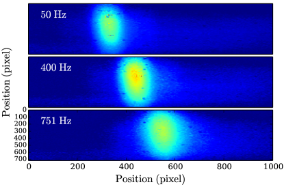
Figure 10: Camera images in Setup 2 at frequencies 50, 400, and 751 Hz.

This change in the width can also be seen in Fig. 11, where we plot the vertically integrated camera images for 17 rotation frequencies as indicated. However, despite the broadening of the profiles, the displacement is clearly visible as the frequency changes.

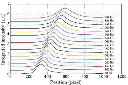
Figure 11: Vertically integrated camera profiles in Setup 2 as a function of the frequency.

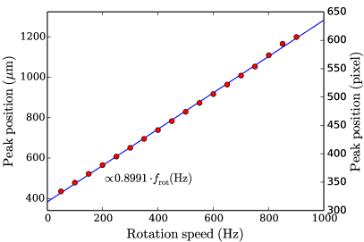
Figure 12: Position of the reflected beam as a function of the rotation speed in Setup 2. On the right vertical axis, the same data are shown in units of the CCD pixels. The linear fit to the peak position is $P_{\mathrm{peak}}(\mathrm{\mu m})=(0.899\pm 0.0059)\cdot f_{\mathrm{rot}}\mathrm{(Hz)}+383.3(\mathrm{\mu m)}$. Error on the data points is not visible.

In Fig. 12 we plot the beam displacement as a function of the rotation speed, similar to Fig.9. The linear fit to these data yields a slope of $(0.899\pm 0.0059)\,\mathrm{\mu m/Hz}$. Given that $d_{1}=4060\pm 1\,\mathrm{mm}$, $d_{2}=730\pm 1\,\mathrm{mm}$, and $d_{3}=3260\pm 1\,\mathrm{mm}$, and considering all error sources, we calculate a speed of light of $c=(3.02\pm 0.03)\cdot 10^{8}\,\mathrm{m/s}$.

Our experimental conditions and results are summarized in Table 1.

	$d_{1}$	$d_{2}$	$d_{3}$	c (m/s)
Setup 1	$\overline{FP-L_{2}}$	$\overline{L_{2}-RM}$	$\overline{RM-SM}$	$2.97\cdot 10^{8}$
	425 mm	1630 mm	4830 mm
Setup 2	$\overline{FP-SM}$	$\overline{SM-RM}$	$\overline{RM-FM}$	$3.02\cdot 10^{8}$
	4060 mm	730 mm	3260 mm

Table 1: Summary of experimental conditions, and results. Overlines denote distances between designated elements.

VI Systematic errors

We have already indicated the magnitude of statistical errors: the calibration of the CCD is about 0.2%, the rotation frequency’s is about 0.3%, the length measurement’s is less than 0.1%, while the Gaussian fits to the profiles contain an error of about 0.2%. However, in addition to these, there are a number of systematical errors that one has to consider.

One we have already pointed out, namely, if the camera is not perpendicular to the laser beam, all displacements will be measured shorter and this will lead to a seemingly larger speed of light. One way of removing this error source is to slightly rotate the camera without moving it, and repeat the measurements multiple times. The smallest value of $c$ should correspond to the perpendicular configuration. However, since this correction is proportional to the cosine of the angle of deviation from the normal, errors are of second order.

Second, if the camera’s plane is not parallel to the axis of the translation stage, the pixel size will be inferred incorrectly, and this, again, will lead to a seemingly higher light speed. As mentioned above, a trivial test for this is the beam profile measured at various positions of the translation stage: all other conditions being identical, a simple translation should result in identical profiles. If this is not the case, then the camera has to be rotated slightly with respect to the translation stage till all measured profiles are identical. As with the systematic error discussed above, corrections are quadratic in the angle.

Third, the measurement of independent quantities, in this case, the frequency (time) and distance might contain errors that result from the particular method used to measure them. Given the accuracy of frequency measurements, it is reasonable to expect that only the value of distance would be affected, and one can safely neglect systematic errors in frequency.

Fourth, imperfections in the focusing lead to small errors. In order to estimate the order of magnitude of these, let us assume that the image of $S$ is formed not at the end mirror, but at $P$, which is at a distance of $x$ from $M$, as shown in Fig. 13. The virtual image of $P$ will also be shifted by the same amount, and following the derivation in Section III., we arrive at

$$c=\frac{4d_{1}d_{3}(d_{3}-x)}{d_{2}+d_{3}-x}\left(\frac{d\Delta s}{d\omega}\right)^{-1}\approx c_{0}\left[1-\frac{xd_{2}}{d_{3}(d_{2}+d_{3})}\right]\ ,$$ (3)

if $x\ll d_{3}$. Note that $d_{1}$ does not necessarily indicate the distance at which the image is formed: it simply designates the position of the measurement (webcam). If $d_{1}$ is chosen such that the imaging condition is not satisfied, it does not mean that the derivation is incorrect, it only means that the image will not be sharp at that point, but Eq.(3) is still valid.

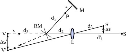
Figure 13: The concept of the measurements, with focusing errors. Notation as in Fig. 1. $P$ is the image of the source $S$.

The magnitude of the correction will depend on two parameters of the setup, $d_{2},d_{3}$, and the inaccuracy in the focusing, $x$. Note that for $d_{2}=0$, i.e., when the rotating mirror is next to the imaging element, the first-oder correction is zero. In the first setup $d_{2}/d_{3}\approx 1/3$, while in the second case, $d_{2}/d_{3}\approx 1/4$. Therefore, an upper bound for the correction in Eq.(3) is $x/(4d_{3})$. Given that $d_{3}\geq 3\,\mathrm{m}$, we incur an error of 1%, if $x\approx 0.12\,\mathrm{m}$. It is reasonable to assume that the focus can be determined with $10\,\mathrm{cm}$ accuracy, even if the imaging elements have such long focal length. Therefore, we can conclude that the error related to imperfect focusing is less than 1%.

Finally, the lens, the only glass element in the first setup, has finite width with a refractive index larger than one, and this adds to the total length between the focal point and the end mirror. This extra optical length can be measured and added to the path, provided the refractive index of the glass is known. Of course, the second setup does not suffer from this kind of error.

VII Conclusion

In conclusion, we presented a simple version of the Foucault method for the measurement of the speed of light. We demonstrated that with readily available and inexpensive optics, and a bit of data processing, acceptable accuracy (results within 1% of the defined value) can be achieved. We also discussed a range of systematic errors, and pointed out several possible improvements. The experiment teaches students the historically important Foucault method, and modern data evaluation concepts at the same time.

Appendix A MATLAB code

Here we list matlab snippets that can be used for the evaluation of images. The usual workflow is to create a profile similar to that in Fig. 8 with the function create_profile, and pass the output to the function fit_profile, which will print the parameters of the best Gaussian fit to the console. gauss simply defines the fit function, and it can easily be replaced by other, more appropriate forms, if necessary.

⬇

function profile = create_profile(fn, range1, range2)

% Returns and displays a profile (a vertically integrated image segment)

%

% Input:

%

% fn: the file (camera image) to read

% range1, range2: the limits of the vertical intagration

im = imread(fn);

im1 = sum(im, 3); % Turns the RGB image into grayscale

figure(1); imagesc(im1)

profile = sum(im1(range1:range2,:));

figure(2); plot(profile, ’ro’);

⬇

function y = gauss(par, xdata)

% Returns a Gaussian function evaluated at points given in xdata

%

% y = A*exp(-(x-x0)^2/sigma^2)+offset

%

% Input:

% par: an array of parameters in the form [A, x0, sigma, offset]

% A: amplitude of the Gaussian

% x0: centre of the Gaussian

% sigma: standard deviation of the Gaussian

% offset: offset of the Gaussian

% xdata: points where the function is to be evaluated

y = par(1) * exp(-(xdata-par(2)).^2/par(3)/par(3)) + par(4);

⬇

function fit_profile(profile, xlim1, xlim2, par)

% Fits a profile with a Gaussian

%

% Input:

% profile: a 1D array of evenly spaced measurement points

% xlim1, xlim2: the fit will be done on domain [xlim1:xlim2]

% par: initial guess of the fit (see gauss(par, xdata))

f = lsqcurvefit(@gauss, par, xlim1:xlim2, profile(xlim1:xlim2))

figure(3); hold on; plot(xlim1:xlim2, profile(xlim1:xlim2), ’ro’)

plot(xlim1:xlim2, gauss(f, xlim1:xlim2), ’b-’);

hold off;

References

- Clark (1956) G. W. Clark, American Journal of Physics 24, 189 (1956).
- Clark (2001) G. W. Clark, American Journal of Physics 69, 110 (2001).
- Belich et al. (1996) T. J. Belich, R. P. Lahm, R. W. Peterson, and C. D. Whipple, American Journal of Physics 65, 186 (1996).
- Lahaye et al. (2012) T. Lahaye, P. Labastie, and R. Mathevet, American Journal of Physics 80, 497 (2012).
- D’Orazio et al. (2010) D. J. D’Orazio, M. J. Pearson, J. T. Schultz, D. Sidor, M. W. Best, K. M. Goodfellow, R. E. Scholten, and J. D. White, American Journal of Physics 78, 524 (2010).
- Dillman (1964) L. T. Dillman, American Journal of Physics 32, 567 (1964).
- Feagin (1979) J. M. Feagin, American Journal of Physics 47, 288 (1979).
- Morrison and Driedger (1980) H. M. Morrison and J. A. Driedger, Physics Education (1980), URL http://iopscience.iop.org/0031-9120/15/2/006.
- Brody et al. (2010) J. Brody, L. Griffin, and P. Segre, American Journal of Physics 78, 650 (2010).
- Rogers et al. (1969) J. Rogers, R. McMillan, R. Pickett, and R. Anderson, American Journal of Physics 37, 816 (1969).
- Deblaquiere et al. (1991) J. A. Deblaquiere, K. C. Harvey, and A. K. Hemann, American Journal of Physics 59, 443 (1991).
- Aoki and Mitsui (2008) K. Aoki and T. Mitsui, American Journal of Physics 76, 812 (2008).
- Ronzani et al. (2008) A. Ronzani, F. Maccarrone, and A. D. Lieto, European Journal of Physics 29, 957 (2008), URL http://iopscience.iop.org/0143-0807/29/5/009.
- Bates (1988) H. E. Bates, American Journal of Physics 56, 682 (1988).