Statistical Estimation: From Denoising to Sparse Regression and Hidden Cliques

Abstract.

These notes review six lectures given by Prof. Andrea Montanari on the topic of statistical estimation for linear models. The first two lectures cover the principles of signal recovery from linear measurements in terms of minimax risk. Subsequent lectures demonstrate the application of these principles to several practical problems in science and engineering. Specifically, these topics include denoising of error-laden signals, recovery of compressively sensed signals, reconstruction of low-rank matrices, and also the discovery of hidden cliques within large networks.

Preface

These lectures provide a gentle introduction to some modern topics in high-dimensional statistics, statistical learning and signal processing, for an audience without any previous background in these areas. The point of view we take is to connect the recent advances to basic background in statistics (estimation, regression and the bias-variance trade-off), and to classical –although non-elementary– developments (sparse estimation and wavelet denoising).

The first three sections will cover these basic and classical topics. We will then cover more recent research, and discuss sparse linear regression in Section 4.3.1, and its analysis for random designs in Section 5.2. Finally, in Section 6.3 we discuss an intriguing example of a class of problems whereby sparse and low-rank structures have to be exploited simultaneously.

Needless to say, the selection of topics presented here is very partial. The reader interested in a deeper understanding can choose from a number of excellent options for further study. Very readable introductions to the fundamentals of statistical estimation can be found in the books by Wasserman [1, 2]. More advanced references (with a focus on high-dimensional and non-parametric settings) are the monographs by Johnstone [3] and Tsybakov [4]. The recent book by Bühlmann and van de Geer [5] provides a useful survey of recent research in high-dimensional statistics. For the last part of these notes, dedicated to most recent research topics, we will provide references to specific papers.

1. Statistical estimation and linear models

1.1. Statistical estimation

The general problem of statistical estimation is the one of estimating an unknown object from noisy observations. To be concrete, we can consider the model

$$y=f(\theta;\text{noise})\,,$$ (1)

where $y$ is a set of observations, $\theta$ is the unknown object, for instance a vector, a set of parameters, or a function. Finally, $f(\,\cdot\,;{\rm noise})$ is an observation model which links together the observations and the unknown parameters which we wish to estimate. Observations are corrupted by random noise according to this model. The objective is to produce an estimation $\widehat{\theta}=\widehat{\theta}(y)$ that is accurate under some metric. The estimation of $\theta$ from $y$ is commonly aided by some hypothesis about the structure, or behavior, of $\theta$. Several examples are described below.

Statistical estimation can be regarded as a subfield of statistics, and lies at the core of a number of areas of science and engineering, including data mining, signal processing, and inverse problems. Each of these disciplines provides some information on how to model data acquisition, computation, and how best to exploit the hidden structure of the model of interest. Numerous techniques and algorithms have been developed over a long period of time, and they often differ in the assumptions and the objectives that they try to achieve. As an example, a few major distinctions to keep in mind are the following.

Parametric versus non-parametric:

In parametric estimation, stringent assumptions are made about the unknown object, hence reducing $\theta$ to be determined by a small set of parameters. In contrast, non-parametric estimation strives to make minimal modeling assumptions, resulting in $\theta$ being an high-dimensional or infinite-dimensional object (for instance, a function).

Bayesian versus frequentist:

The Bayesian approach assumes $\theta$ to be a random variable as well, whose ‘prior’ distribution plays an obviously important role. From a frequentist point of view, $\theta$ is instead an arbitrary point in a set of possibilities. In these lectures we shall mainly follow the frequentist point of view, but we stress that the two are in fact closely related.

Statistical efficiency versus computational efficiency:

Within classical estimation theory, a specific estimator $\widehat{\theta}$ is mainly evaluated in terms of its accuracy: How close (or far) is $\widehat{\theta}(y)$ to $\theta$ for typical realizations of the noise? We can broadly refer to this figure of merit as to ‘statistical efficiency.’

Within modern applications, computational efficiency has arisen as a second central concern. Indeed $\theta$ is often high-dimensional: it is not uncommon to fit models with millions of parameters. The amounts of observations has grown in parallel. It becomes therefore crucial to devise estimators whose complexity scales gently with the dimensions, and with the amount of data.

We next discuss informally a few motivating examples.

1.1.1. Example 1: Exploration seismology

Large scale statistical estimation plays a key role in the field of exploration seismology. This technique uses seismic measurements on the earth surface to reconstruct geological structures, composition and density field of a geological substrates in [6]. Measurements are acquired, generally, by sending some known seismic wave through the ground, perhaps through a controlled explosive detonation, and measuring the response at multiple spatially dispersed sensors.

Below is a simple dictionary that points at the various elements of the model (1) in this example.

Exploration Seismology
$y$	seismographic measurements
$\theta$	earth density field
Hypothesis	smooth density field

The function $f(\,\cdots\,)$ in Eq. (1) expresses the outcome of the seismographic measurements, given a certain density field $\theta$ and a certain source of seismic waves (left implicit since it is known). While this relation is of course complex, and ultimately determined by the physics of wave propagation, it is in principle perfectly known.

Because of the desired resolution of the recovered earth density field, this statistical estimation problem is often ill-posed, as sampling is severely limited by the cost of generating the source signal and the distribution and set-up of the receivers. Resolution can be substantially improved by using some structural insights into the nature of the earth density field. For instance, one can exploit the fact that this is mostly smooth with the exception of some discontinuity surfaces.

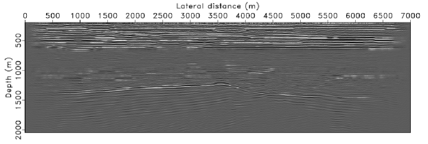
Figure 1. A recovered earth density field, from [6].

1.1.2. Example 2: Hidden structure in networks

Many modern data sets are relational, i.e. they express pairwise relations within a set of objects. This is the case in social networks, communication networks, unsupervised learning and so on.

In the simplest case, for each pair of nodes in a network, we know whether they are connected or not. Finding a hidden structure in such a network is a recurring problem with these datasets. A highly idealized but nevertheless very interesting problem requires to find a highly connected subgraph in a otherwise random graph.

Hidden Network Structure
$y$	large network
$\theta$	hidden subset of nodes
Hypothesis	hidden network is highly connected

From Figure 2, it is apparent that the discovery of such networks can be a difficult task.

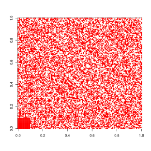
(a) Subgraph easily visible.

(b) Subgraph hidden.

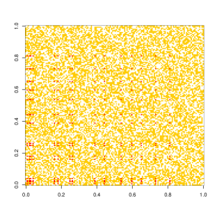
(c) Subgraph revealed

Figure 2. The same network adjacency matrix, is shown in (a) and (b), but the nodes permuted in (b). In (c), the hidden subgraph is revealed.

1.1.3. Example 3: Collaborative filtering

Recommendation systems are ubiquitous in e-commerce and web services. They aim at personalizing each user’s experience through an analysis of her past behavior, and –crucially– the past behavior of similar users. The algorithmic and statistical techniques that allow to exploit this information are referred to as ‘collaborative filtering.’ Amazon, Netflix, YouTube all make intensive use of collaborative filtering technologies.

In a idealized model for collaborative filtering, each user of a e-commerce site is associated to a row of a matrix, and each product to a column. Entry $\theta_{i,j}$ in this matrix corresponds to the evaluation that user $i$ gives of product $j$. A small subset of the entries is observed because of feedback provided by the users (reviews, ratings, purchasing behavior). In this setting, collaborative filtering aims at estimating the whole matrix, on the basis of noisy observations of relatively few of its entries.

While this task is generally hopeless, it is observed empirically that such data matrices are often well approximated by low-rank matrices. This corresponds to the intuition that a small number of factors (corresponding to the approximate rank) explain the opinions of many users concerning many items. The problem is then modeled as the one of estimating a low-rank matrix from noisy observations of some of its entries.

Collaborative Filtering
$y$	small set of entries in a large matrix
$\theta$	unknown entries of matrix
Hypothesis	matrix has a low-rank representation

A toy example of this problem is demonstrated in Figures 4-4. It can be observed that an accurate estimation of the original matrix is possible even when very few of its coefficients are known.

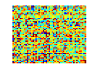
(a) low-rank matrix $M$

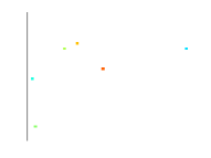
(b) sampled matrix $M^{\mathbb{E}}$

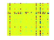
(c) output $\hat{M}$

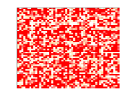
(d) squared error $\left(M-\hat{M}\right)^{2}$

Figure 3. Recovering a $2000\times 2000$ rank-8 matrix from $0.25\%$ of its values.

(a) low-rank matrix $M$

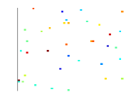
(b) sampled matrix $M^{\mathbb{E}}$

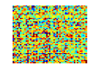
(c) output $\hat{M}$

(d) squared error $\left(M-\hat{M}\right)^{2}$

Figure 4. Recovering a $2000\times 2000$ rank-8 matrix from $1.75\%$ of its values.

1.2. Denoising

We will begin by considering in greater depth a specific statistical estimation problem, known as ‘denoising.’ One the one hand, denoising is interesting, since it is a very common signal processing task: In essence, it seeks restore a signal which has been corrupted by some random process, for instance additive white-noise. On the other, it will allow us to introduce some basic concepts that will play an important role throughout these lectures. Finally, recent research by [7] has unveiled a deep and somewhat surprising connection between denoising and the rapidly developing field of compressed sensing.

To formally define the problem, we assume that the signal to be estimated is a function $t\mapsto f(t)$ Without loss of generality, we will restrict the domain of $f(t)$, $f:\left[0,1\right]\rightarrow$. We measure $n$ uniformly-spaced samples over the domain of $f$,

$$y_{i}=f\left(i/n\right)+w_{i}~{},$$ (2)

where $i\in\left\{1,2,\dots,n\right\}$ is the sample index, and $w_{i}\sim\mathcal{N}\left(0,\sigma^{2}\right)$ is the additive noise term. Each of $y_{1},\dots y_{n}$ is a sample.

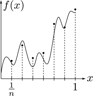
Figure 5. Depiction of a discrete-time sampling of the continuous-time function, $f(x)$. Notice that the additive noise term, $w_{i}$, prevents exact knowledge of $f(i/n)$.

For the denoising problem, we desire to calculate the original function from the noise-corrupted observables $y_{i}$. How might we go about doing this?

1.3. Least Squares (LS) estimation

The Least Squares Method dates back to Gauss and Legendre [8].

A natural first idea is to parametrize the function $f$. For instance we can tentatively assume that it is a degree $p-1$ polynomial

$$f(t)=\displaystyle\sum\limits_{j=1}^{p}\theta_{j}~{}t^{j-1}.$$ (3)

Each monomial is weighted according to coefficient $\theta_{j}$ for $j\in\left\{1,2,\dots,p\right\}$, and we will collect these coefficients in a vector $\theta=(\theta_{1},\theta_{2},\dots,\theta_{p})\in^{p}$. Thus, the problem of recovering $f(t)$ boils down to the recovery of the $p$ coefficients $\theta_{j}$ from the set of observables, $y_{i}$. We therefore seek to find the set of coefficients which which generate a function that most closely matches the observed samples.

It is natural to set this up as an optimization problem (here RSS stands for ‘residual sum of squares’)

$$\widehat{\theta}^{{\mbox{\rm\tiny LS}}}(y) \equiv\operatorname*{argmin}_{\theta}~{}~{}\text{RSS}(\theta),$$ (4)

$$\text{RSS}(\theta) \equiv~{}\displaystyle\sum\limits_{i=1}^{n}\left(y_{i}-\displaystyle\sum\limits_{j=1}^{p}\theta_{j}\left(\frac{i}{n}\right)^{j-1}\right)^{2}.$$ (5)

Fitting a low-degree polynomial to a dataset by least squares is a very common practice, and the reader has probably tried this exercise at least once. A moment reflection reveals that nothing is special about the polynomials used in this procedure. In general, we can consider a set of functions $\{\varphi_{1},\varphi_{2},\dots,\varphi_{p}\}$, where

$$\varphi_{j}:[0,1]\rightarrow.$$ (6)

Of course, the quality of our estimate depends on how well the functions $\{\varphi_{j}\}$ capture the behavior of the signal $f$. Assuming that $f$ can be represented as a linear combination of these functions, we can rewrite our model as

$$y_{i} =\displaystyle\sum\limits_{j=1}^{p}\theta_{0j}\varphi_{j}\left(i/n\right)+w_{i}.$$ (7)

Equivalently, if we define $\varphi:[0,1]\to^{p}$ by letting $\varphi(x)=(\varphi_{1}(x),\varphi_{2}(x),\dots,\varphi_{p}(x))$, $\theta_{0}=(\theta_{0,1},\theta_{0,2},\dots,\theta_{0,p})$, and denoting by $\langle a,b\rangle\equiv\sum_{i=1}^{m}a_{i}b_{i}$ the usual scalar product in ^m, we have

$$y_{i} =\langle\theta_{0},\varphi(i/n)\rangle+w_{i}.$$ (8)

Before continuing further, it is convenient to pass to matrix notation. Let us define a matrix ${\mathbf{X}}\left(X_{ij}\right)\in^{n\times p}$ whose entry $i,j$ is given by

$$X_{ij} =\varphi_{j}\left(\frac{i}{n}\right),$$ (9)

Using this notation, and letting $y=(y_{1},y_{2},\dots,y_{n})$, $w=(w_{1},w_{2},\dots,w_{n})$, our model reads

$$y=X\theta_{0}+w\,,$$ (10)

$w\sim\mathcal{N}\left(0,\sigma^{2}{\rm I}_{n}\right)$ (here and below ${\rm I}_{n}$ denotes the identity matrix in $n$ dimensions: the subscript will be dropped if clear from the context).

From (10), we see that vector of observations $y$ is approximated as a linear combination of the columns of ${\mathbf{X}}$, each columns corresponding to one of the functions $\varphi_{1},\varphi_{2},\dots,\varphi_{p}$, evaluated on the sampling points.

This is a prototype of a very general idea in statistical learning, data mining and signal processing. Each data point $x$ (or each point in a complicated space, e.g. a space of images) is represented by a vector in ^p. This vector is constructed by evaluating $p$ functions at $x$ hence yielding the vector $(\varphi_{1}(x),\varphi_{2}(x),\dots,\varphi_{p}(x))$. Of course, the choice suitable functions $\{\varphi_{j}\}$ is very important and domain-specific.

The functions $\{\varphi_{j}\}$ (or –correspondingly– the columns of the matrix ${\mathbf{X}}$) have a variety of names. They are known as “covariates” and “predictors” in statistics, as “features” in the context of machine learning and pattern recognition. The set of features $\{\varphi_{j}\}$ is sometimes called a “dictionary,” and the matrix ${\mathbf{X}}$ is also referred to as the “design matrix.” Finding an appropriate set of features, i.e. “featurizing”, is a problem of its own. The observed $y_{i}$ are commonly referred to as the “responses” or “labels” within statistics and machine-learning, respectively. The act of finding the true set of coefficients $\theta_{0}$ is known as both “regression” and “supervised learning”.

So, how do we calculate the coefficients $\theta_{0}$ from $y$? Going back to least squares estimation, we desire to find a set of coefficients, $\widehat{\theta}$ which best match our observations. Specifically, in matrix notation (4) reads

$$\widehat{\theta}^{{\mbox{\rm\tiny LS}}}=\operatorname*{argmin}_{\theta\in^{p}}~{}~{}\mathcal{L}(\theta),$$ (11)

where

$$\mathcal{L}(\theta) =\frac{1}{2n}\|y-{\mathbf{X}}\theta\|_{2}^{2},$$

$$=\frac{1}{2n}\displaystyle\sum\limits_{i=1}^{n}\left(y_{i}-\left<x_{i},\theta\right>\right)^{2},$$ (12)

with $x_{i}$ the $i$-th row of ${\mathbf{X}}$. Here and below $\|a\|_{2}$ denotes the $\ell_{2}$-norm of vector $a$: $\|a\|_{2}^{2}=\displaystyle\sum\limits_{i}a_{i}^{2}$. The minimizer can be found by noting that

$$\nabla\mathcal{L}(\theta) =-\frac{1}{n}{\mathbf{X}}^{\sf T}(y-{\mathbf{X}}\theta),$$ (13)

$$\therefore~{}~{}~{}~{}\widehat{\theta}^{{\mbox{\rm\tiny LS}}} =\left({\mathbf{X}}^{\sf T}{\mathbf{X}}\right)^{-1}{\mathbf{X}}^{\sf T}y.$$ (14)

Looking at (14), we note that an important role is played by the sample covariance matrix

$$\widehat{\Sigma}=\frac{1}{n}{\mathbf{X}}^{T}{\mathbf{X}}.$$ (15)

This is the matrix of correlations of the predictors $\{\varphi_{1},\dots,\varphi_{p}\}$. The most immediate remark is that, for $\widehat{\theta}^{{\mbox{\rm\tiny LS}}}$ to be well defined, $\widehat{\Sigma}$ needs to be invertible, which is equivalent to require $\text{rank}\left({\mathbf{X}}\right)=p$. This of course can only happen if the number of parameter is no larger than the number of observations: $n\leq p$. Of course, if $\widehat{\Sigma}$ is invertible but is nearly-singular, then $\widehat{\theta}$ will be very unstable and hence a poor estimator. A natural way to quantify the ‘goodness’ of $\widehat{\Sigma}$ is through its condition number $\kappa(\widehat{\Sigma})$, that is the ratio of its largest to its smallest eigenvalue: $\kappa(\widehat{\Sigma})=\lambda_{\rm max}(\widehat{\Sigma})/\lambda_{\rm min}(\widehat{\Sigma})$. From this point of view, an optimal design has minimal condition number $\kappa(\widehat{\Sigma})=1$, which corresponds to ${\mathbf{X}}$ to be proportional to an orthogonal matrix. In this case ${\mathbf{X}}$ is called an ‘orthogonal design’ and we shall fix normalizations by assuming $\widehat{\Sigma}=({\mathbf{X}}^{{\sf T}}{\mathbf{X}}/n)={\rm I}_{p}$

In functional terms, we see that the LS estimator is calculated according to the correlations between $y$ and the predictors,

$$\widehat{\Sigma}_{jl} =\frac{1}{n}\displaystyle\sum\limits_{i=1}^{n}\varphi_{j}\left(i/n\right)\varphi_{l}\left(i/n\right),$$ (16)

$$\therefore~{}~{}~{}~{}\widehat{\theta}^{{\mbox{\rm\tiny LS}}}_{l} =\displaystyle\sum\limits_{j=1}^{p}\left(\widehat{\Sigma}^{-1}\right)_{lj}\left(\frac{1}{n}\displaystyle\sum\limits_{i=1}^{n}\varphi_{j}(i/n)y_{i}\right).$$ (17)

1.4. Evaluating the estimator

Now that we calculated the LS estimator for our problem, a natural question arises: is this indeed the best estimator we could use? In order to answer this question, we need a way of comparing one estimator to another.

This is normally done by considering the risk function associated with the estimator. If the model depends on a set of parameters $\theta\in^{p}$, the risk function is a function $R:^{p}\to$, defined by

$$R(\theta) =\mathbb{E}\left\{\|\widehat{\theta}(y)-\theta\|_{2}^{2}\right\},$$

$$=\displaystyle\sum\limits_{j=1}^{p}\mathbb{E}\left\{(\hat{\theta}_{j}(y)-\theta_{j})^{2}\right\}.$$ (18)

Here expectation is taken with respect to $y$, distributed according to the model (10) with $\theta_{0}=\theta$. Note that the $\ell_{2}$-distance is used to measure the estimation error.

Other measures (called ‘loss functions’) could be used as well, but we will focus on this for the sake of concreteness. We can also calculate risk over the function space and not just over the parameter space. This is also known as the ‘prediction error’:

$$R_{{\rm p}}(\theta) =\frac{1}{n}\displaystyle\sum\limits_{i=1}^{n}\mathbb{E}\left\{\left(\widehat{f}\left(i/n\right)-f\left(i/n\right)\right)^{2}\right\},$$

$$=\frac{1}{n}\displaystyle\sum\limits_{i=1}^{n}\mathbb{E}\left\{\left[\displaystyle\sum\limits_{j=1}^{p}{\mathbf{X}}_{ij}\left(\hat{\theta}_{j}-\theta_{j}\right)\right]^{2}\right\},$$

$$=\frac{1}{n}\mathbb{E}\left\{\|{\mathbf{X}}\left(\hat{\theta}-\theta\right)\|_{2}^{2}\right\}.$$ (19)

In particular, for ${\mathbf{X}}$ an orthogonal design, $R_{{\rm p}}(\theta)=c\,R(\theta)$.

Let us apply this definition of risk to the LS estimator, $\hat{\theta}^{{\mbox{\rm\tiny LS}}}$. Returning to the signal sampling model,

$$y ={\mathbf{X}}\theta_{0}+w.$$ (20)

$$\therefore~{}~{}~{}~{}\widehat{\theta}^{{\mbox{\rm\tiny LS}}} =\left({\mathbf{X}}^{{\sf T}}{\mathbf{X}}\right)^{-1}{\mathbf{X}}^{{\sf T}}y,$$

$$=\theta_{0}+({\mathbf{X}}^{{\sf T}}{\mathbf{X}})^{-1}{\mathbf{X}}^{{\sf T}}w,$$ (21)

which shows that the LS estimator will return the true parameters, $\theta_{0}$, perturbed by some amount due to noise. Now, we will calculate the risk function

$$R(\theta) =\mathbb{E}\left\{\|\widehat{\theta}^{{\mbox{\rm\tiny LS}}}(y)-\theta_{0}\|_{2}^{2}\right\},$$

$$=\mathbb{E}\left\{\|\left({\mathbf{X}}^{{\sf T}}{\mathbf{X}}\right)^{-1}{\mathbf{X}}^{{\sf T}}w\|_{2}^{2}\right\},$$

$$=\mathbb{E}\left\{w^{{\sf T}}{\mathbf{X}}\left({\mathbf{X}}^{{\sf T}}{\mathbf{X}}\right)^{-2}{\mathbf{X}}^{{\sf T}}w\right\},$$

$$=\sigma^{2}\text{Tr}\left({\mathbf{X}}\left({\mathbf{X}}^{{\sf T}}{\mathbf{X}}\right)^{-2}{\mathbf{X}}^{{\sf T}}\right),$$

$$=\sigma^{2}\text{Tr}\left(\left({\mathbf{X}}^{{\sf T}}{\mathbf{X}}\right)^{-1}\right),$$

$$=\frac{\sigma^{2}p}{n}\left[\frac{\text{Tr}\left(\widehat{\Sigma}^{-1}\right)}{p}\right],$$ (22)

where we add the $p$ term to the final result because we expect that $\frac{1}{p}\text{Tr}\left(\widehat{\Sigma}^{-1}\right)$ to be on the order one, under the assumption of near-orthonormal predictors.

Tho further illustrate this point, let us consider the case in which the functions $\{\varphi_{j}\}$ are orthonormal (more precisely, they are an orthonormal set in $L^{2}([0,1])$). This means that

$$\int_{0}^{1}\varphi_{i}(x)\varphi_{j}(x)\,{\rm d}x=\delta_{ij}\,.$$ (23)

where $\delta{ij}$ is $1$ when $i=j$ and $0$ for all $i\neq j$. For $n$ large, this implies

$$\widehat{\Sigma}_{jl}=\frac{1}{n}\displaystyle\sum\limits_{i=1}^{n}\varphi_{j}\left(i/n\right)\varphi_{l}\left(i/n\right)\approx\delta_{jl},$$ (24)

where we assumed that the sum can be approximated by an integral. In other words, if the functions $\{\varphi_{j}\}$ are orthonormal, the design is nearly orthogonal, and this approximation gets better as the number of samples increases. Thus, in such good conditions, $\text{Tr}\left(\widehat{\Sigma}^{-1}\right)\approx p$. Under these conditions, we can simplify the risk function for the LS estimator in the case of orthonormal or near-orthonormal predictors to be,

$$R(\theta)\approx\frac{p\sigma^{2}}{n}.$$ (25)

This result has several interesting properties:

• The risk is proportional to the noise variance. This makes sense: the larger is noise, the worst we can estimate the function.

• It is inversely proportional to the number of samples $n$: the larger is the number of observations, the better we can estimate $f$.

• The risk is proportional to the number of parameters $p$. This fact can be interpreted as an over-fitting phenomenon If we choose a large $p$, then our estimator will be more sensitive to noise. Conversely, we are effectively searching the right parameters in a higher-dimensional space, and a larger number of samples is required to determine it the same accuracy.

• The risk $R(\theta)$ is independent of $\theta$. This is closely related to the e linearity of the LS estimator.

At this point, two questions arise naturally:

1. Is this the best that we can do? Is it possible to use a different estimator and decrease risk?

2. What happens if the function to be estimated is function is not exactly given by a linear combinations of the predictors? Indeed in general, we cannot expect to have a perfect model for the signal, and any set of predictors is only approximate:

   $$f(t)\neq\sum_{j=1}^{p}\theta_{j}\varphi_{j}(t).$$ (26)

To discuss these two issues, let us first change the notation for the risk function, by making explicit the dependence on the estimator $\widehat{\theta}$:

$$R(\theta;\widehat{\theta})\quad\text{where}\quad \theta\in^{p},$$ (27)

$$\hat{\theta}:^{n}\rightarrow^{p}.$$

Note that estimators, $\widehat{\theta}$, are functions of $y\in^{n}$. For two estimators, $\widehat{\theta}^{1}$ and $\widehat{\theta}^{2}$, we can compare $R(\theta;\widehat{\theta}^{1})$ and $R(\theta;\widehat{\theta}^{2})$. This leads to the next, crucial question: how do we compare these two curves? For instance, in Figure 6 we sketch two cartoon risk functions $R(\theta;\widehat{\theta}^{1})$ and $R(\theta;\widehat{\theta}^{2})$. Which one is the best one? The way this question is answered has important consequences.

Note that naively, one could hope to find an estimator that is simultaneously the best at all points $\theta$. Letting this ideal estimator be denoted by $\widehat{\theta}^{\text{opt}}$, we would get

$$R(\theta;\widehat{\theta}^{\text{opt}})\leq R(\theta;\widehat{\theta})\quad\forall~{}\theta,\widehat{\theta}.$$ (28)

However, assuming the existence of such an ideal estimator leads to a contradiction. To see this, we will let the predictors be, for simplicity

$${\mathbf{X}}=\sqrt{n}{\rm I}_{n}\,,\quad\quad p=n,$$ (29)

which means our regression problem is now

$$y=\theta+\frac{w}{\sqrt{n}},\quad\quad w\sim\mathcal{N}(0,\sigma^{2}{\rm I}_{n}).$$ (30)

Note that in this case the LS estimator is simply $\widehat{\theta}^{{\mbox{\rm\tiny LS}}}(y)=y$.

Next, fix $\xi\in^{p}$, and consider the oblivious estimator that always returns $\xi$:

$$\widehat{\theta}^{\xi}(y)=\xi\,.$$ (31)

This has the risk function

$$R(\theta;\widehat{\theta}^{\xi})=\|\xi-\theta\|_{2}^{2}.$$ (32)

If an ‘ideal’ estimator $\widehat{\theta}^{\text{opt}}$ as above existed, it would beat $\widehat{\theta}^{\xi}$, which implies in particular

$$R(\xi;\widehat{\theta}^{\text{opt}})=0\,.$$ (33)

Since $\xi$ is arbitrary, this would imply that the ideal estimator has risk everywhere equal to $0$, i..e. always reconstruct the true signal perfectly, independently of the noise. This is of course impossible.

One approach would be to evaluate the Bayes risk, which would compute the expected value of each risk curve dependent upon the prior distribution of the parameters, $\text{Pr}[\theta]$. However, it is not clear in every case how one might determine this prior, and its choice can completely skew the comparison between $\hat{\theta}^{1}$ and $\hat{\theta}^{2}$.

Figure 6. Comparing the risk functions of two different estimators, $\hat{\theta}^{1}$, $\hat{\theta}^{2}$ over the space of possible parameters, $\theta$. Also shown is a risk function for some estimator which is ideal in the sense that it is below both both of the known estimators for all $\theta$.

Figure 7. Any arbitrary trivial estimator can minimize the point-wise risk at point $\xi$.

One approach to overcome this problem is to evaluate for each risk function the corresponding ‘Bayes risk.’ This amounts to averaging $R(\theta;\widehat{\theta})$ over $\theta$, using a certain prior distribution of the parameters $\text{P}(\theta)$. Namely

$$R_{B}({\rm P};\widehat{\theta})\equiv\int~{}R(\theta;\widehat{\theta})\;{\rm P}({\rm d}\theta).$$ (34)

However, it is not clear in every case how one might determine this prior. Further, the choice of $\text{P}(\theta)$ can completely skew the comparison between $\widehat{\theta}^{1}$ and $\widehat{\theta}^{2}$. If $\text{P}(\theta)$ is concentrated in a region in which –say– $\widehat{\theta}^{1}$ is superior to $\widehat{\theta}^{2}$, then $\widehat{\theta}^{1}$ will obviously win the comparison, and viceversa.

In the next section we shall discuss the minimax approach to comparing estimators.

2. Nonlinear denoising and sparsity

2.1. Minimax risk

The previous lecture discussed estimating a set of parameters, $\theta$, given the linear model

$$y={\mathbf{X}}\theta+w.$$ (35)

In this discussion, we stated that there exists no estimator which dominates all other possible estimators in terms of risk, $R(\theta;\widehat{\theta})$. Still the question remains of how to compare two different estimators $\widehat{\theta}^{1}$, $\widehat{\theta}^{2}$.

Figure 8. The risk of an unknown estimator which dominates $\hat{\theta}^{LS}$ for all $\theta$.

A fruitful approach to this question is to consider the worst case risk over some region $\Omega\subseteq^{p}$. Formally, we define the minimax risk of $\widehat{\theta}$ over $\Omega$ as

$$R_{*}(\Omega;\widehat{\theta})=\sup_{\theta\in\Omega}~{}R(\theta;\widehat{\theta}).$$ (36)

Such a definition of risk is useful if we have some knowledge a priori about the region in which the true parameters live. The minimax risk allows us to compare the maximal risk of a given estimator over the set $\Omega$ to find an estimator with minimal worst case risk. The minimax risk is also connected to the Bayes risk which we defined earlier,

$$R_{B}({\rm P};\widehat{\theta}) \equiv\int~{}R(\theta;\widehat{\theta})\;{\rm P}({\rm d}\theta)\,,$$ (37)

$$R_{*}(\Omega;\widehat{\theta}) =\sup_{\text{supp}({\rm P})\subseteq\Omega}R_{B}({\rm P};\widehat{\theta}).$$ (38)

With this definition of minimax risk, it is easy do compute the minimax risk of least squares

$$R_{*}(^{p};\widehat{\theta}^{{\mbox{\rm\tiny LS}}})=\frac{p\sigma^{2}}{n}\left[\frac{\text{Tr}(\hat{\Sigma}^{-1})}{p}\right],.$$ (39)

The least squares estimator is optimal in minimax sense.

Theorem 1.

The least squares estimator is minimax optimal over ^p. Namely, any estimator $\widehat{\theta}$ has minimax risk $R_{*}(^{p};\widehat{\theta})\geq R_{*}(^{p};\widehat{\theta}^{{\mbox{\rm\tiny LS}}})$.

Proof.

The proof of this result relies on the connection with Bayes risk. Consider for the sake of simplicity the case of orthogonal designs, $\widehat{\Sigma}={\rm I}$. It is not hard to show that, if ${\rm P}$ is gaussian with mean $0$ and covariance $c^{2}{\rm I}_{p}$, then

$$\inf_{\widehat{\theta}}R_{B}({\rm P};\widehat{\theta}) =\frac{c^{2}\sigma^{2}}{c^{2}+\sigma^{2}}\,.$$ (40)

Hence, for any estimator $\widehat{\theta}$

$$\sup_{\theta\in^{p}}R(\theta;\widehat{\theta})\geq R_{B}({\rm P};\widehat{\theta})\geq\frac{c^{2}\sigma^{2}}{c^{2}+\sigma^{2}}\,.$$ (41)

Since $c$ is arbitrary, we can let $c\to\infty$, whence

$$R_{*}(^{p};\widehat{\theta})\geq\sigma^{2}\,.$$ (42)

A full treatment of a more general result can be found, for instance in [2, Chapter 7]. ∎

A last caveat. One might suspect –on the grounds of the last theorem– that least squares estimation is optimal ‘everywhere’ in ^p. This was indeed common belief among statisticians until the surprising discovery of the ‘Stein phenomenon’ in the early sixties [9]. In a nutshell, for $p\geq 3$ there exist estimators that have risk $R(\theta;\widehat{\theta})<R(\theta;\widehat{\theta}^{{\mbox{\rm\tiny LS}}})$ strictly for every $\theta\in^{p}$! (The gap vanishes as $\theta\to\infty$.) We refer to [2, Chapter 7] for further background on this.

2.2. Approximation error and the bias-variance tradeoff

Until now we have assumed that the unknown function$f(t)$, could be exactly represented by the set of predictors, corresponding to columns of ${\mathbf{X}}$. How is our ability to estimate the parameters set $\theta$, and thus $f(t)$, affected when this assumption is violated?

In order to study this case, we assume that we are given an infinite sequence of predictors $\{\varphi_{j}\}_{j\geq 1}$, and use only the first $J$ to estimate $f$. For any fixed $J$, $f(t)$ can be approximated as a linear combination of the first $J$ predictors, plus an error term which is dependent upon $J$

$$f(t)=\displaystyle\sum\limits_{j=1}^{J}\theta_{j}\varphi_{j}(t)+\Delta_{J}(t).$$ (43)

For a complete set $\{\varphi_{j}\}$, we can ensure $\lim_{J\to\infty}\|\Delta_{J}\|=0$ in a suitable norm. This can be formalized by assuming $\{\varphi_{j}\}_{j\geq 1}$ to be a orthonormal basis in the Hilbert space $L^{2}([0,1])$ and the above to be the orthonormal decomposition. In particular, the remainder will be orthogonal to the expansion,

$$\int_{0}^{1}~{}\Delta_{J}(t)\varphi_{j}(t)\,{\rm d}t=0\quad\forall j\in\{1,\dots,J\}\,.\$$ (44)

Alternatively, we can require orthogonality with respect to the sampled points (the resulting expansions are very similar for $n$ large)

$$\frac{1}{n}\displaystyle\sum\limits_{i=1}^{n}\Delta_{J}\left(i/n\right)\varphi_{j}\left(i/n\right)=0\quad\forall j\in\{1,2,\dots,J\}.$$ (45)

With the remainder $\Delta_{J}$, our regression model becomes

$$y={\mathbf{X}}\theta_{0}+\Delta_{J}+w,$$ (46)

where ${\mathbf{X}}\in^{n\times J}$, $w\sim\mathcal{N}\left(0,\sigma^{2}I_{n}\right)$, and ${\mathbf{X}}^{T}\Delta_{J}=0$. Recall, the LS estimator is given by

$$\widehat{\theta} =({\mathbf{X}}^{T}{\mathbf{X}})^{-1}{\mathbf{X}}^{T}y,$$

$$=\theta_{0}+({\mathbf{X}}^{T}{\mathbf{X}})^{-1}{\mathbf{X}}^{T}w.$$ (47)

We can compute the prediction risk as follows

$$R_{p}(f) =~{}\frac{1}{n}~{}\mathbb{E}\left\{\displaystyle\sum\limits_{i=1}^{n}\Big{(}\hat{f}\left(i/n\right)-f\left(i/n\right)\Big{)}^{2}\right\},$$

$$=~{}\frac{1}{n}~{}\mathbb{E}\left\{\|{\mathbf{X}}\widehat{\theta}-{\mathbf{X}}\theta_{0}-\Delta_{J}\|_{2}^{2}\right\},$$

$$=~{}\frac{1}{n}~{}\mathbb{E}\left\{\|{\mathbf{X}}(\theta-\widehat{\theta}_{0})\|_{2}^{2}\right\}+\frac{1}{n}\|\Delta_{J}\|_{2}^{2},$$

$$=~{}\frac{1}{n}~{}\mathbb{E}\left\{\|{\mathbf{X}}({\mathbf{X}}^{T}{\mathbf{X}})^{-1}{\mathbf{X}}^{T}w\|_{2}^{2}\right\}+\frac{1}{n}\|\Delta_{J}\|_{2}^{2},$$

$$=~{}\frac{1}{n}~{}\|\Delta_{J}\|_{2}^{2}+\frac{\sigma^{2}}{n}\text{Tr}\left({\mathbf{X}}({\mathbf{X}}^{T}{\mathbf{X}})^{-1}{\mathbf{X}}^{T}\right).$$ (48)

Finally, note that ${\mathbf{X}}({\mathbf{X}}^{T}{\mathbf{X}})^{-1}{\mathbf{X}}^{T}\in^{n\times n}$ is the orthogonal projector o the space spanned by the columns of ${\mathbf{X}}$. Hence its trace is always equal to $J$.This gives us the final form of the estimation risk at $f(\,\cdot\,)$, as a function of $J$,

$$R_{p}(f)=\frac{\|\Delta_{J}\|_{2}^{2}}{n}+J\frac{\sigma^{2}}{n}.$$ (49)

In other words, the estimation risk associated with $f(\,\cdot\,)$ is a sum of two terms, both of which are dependent upon the choice of $J$:

• The first term is associated with the approximation error induced by the choice of the predictor $\{\varphi_{j}\}$. It is independent of the noise variance $\sigma^{2}$, decreases with $J$.

  We interpret it therefore a bias term.

• The second term depends on the noise level, and is related to the fluctuations that the noise induces in $\widehat{\theta}$. It increases with the number of predictors $J$, as the fi becomes more unstable.

  We interpret it therefore as a variance term.

Therefore, the optimal number of predictors to use, $J^{*}$ is the one which minimizes the risk by striking a balance between bias and variance. In other words, we want to find the optimal point between under- and over-fitting the model. Note that how we choose the predictors themselves determines the rate at which the bias term goes to zero as $J$ increases.

Figure 9. The effect of bias and variance on estimation risk.

2.2.1. Example: The Fourier basis

In this example we select our set of predictors to be a Fourier basis

$$\varphi_{j}(t)=\sqrt{2}\cos((j-1)\pi t),$$ (50)

for $t\in[0,1]$. If $f(\,\cdot\,)$ is square-integrable, then it can be represented as an infinite series (converging in $L^{2}([0,1])$, i.e. in mean square error)

$$f(t)=\displaystyle\sum\limits_{j=1}^{\infty}\theta_{0j}\varphi_{j}(t).$$ (51)

However, if only $J$ sinusoids are used, the remainder, $\Delta_{J}$ is

$$\Delta_{J}(t)=f(t)-\displaystyle\sum\limits_{j=1}^{J}\theta_{0j}\varphi_{j}(t).$$ (52)

And, finally, the squared norm of $\Delta_{J}$ is, by orthogonality

$$\|\Delta_{J}\|^{2}_{2} =\sum_{i=1}^{n}\Delta_{J}(i/n)^{2},$$

$$\approx n\int_{0}^{2}\Delta_{J}(t)^{2}=n\int\displaystyle\sum\limits_{j=J+1}^{\infty}\theta_{0j}^{2}.$$ (53)

Here we replaced the sum by an integral, an approximation that is accurate for $n$ large.

Note that the decay of the bias term mirrors the decay of the Fourier coefficients of $f$, by (53). In particular, if $f$ is smooth, its Fourier coefficients decay faster, and hence the bias decays rapidly with $J$. In this case, the Fourier basis is a good set of features/predictors (a good dictionary) for our problem.

Figure 10. Depiction of the rate of decay of the bias term as a function of $J$.

We now look at the case of Fourier predictors for a specific class od smooth functions, namely functions whose second derivative is square integrable. Formally we define

$$W(C)\equiv\left\{\int_{0}^{1}\left(f^{\prime\prime}\left(t\right)\right)^{2}\,{\rm d}t\leq C^{2}\right\}\,,$$ (54)

and we will consider estimation over $\Omega=W(C)$. This space is known in functional analysis as the ‘Sobolev ball of radius $C$ and order $2$.’

In terms of Fourier coefficients, this set of smooth functions can be characterized as

$$\int_{0}^{1}\left(\displaystyle\sum\limits_{j=1}^{\infty}\pi^{2}(j-1)^{2}\theta_{0j}\varphi_{j}(t)\right)^{2}{\rm d}t\leq C$$ (55)

Or equivalently

$$\displaystyle\sum\limits_{j=1}^{\infty}\pi^{4}(j-1)^{4}\theta_{0j}^{2}\leq C.$$ (56)

Now, in order for this to happen, we must have (56) is satisfied,

$$\sum_{j=J+1}^{\infty}\theta_{0j}^{2}\lesssim\frac{C^{\prime}}{J^{4}},$$ (57)

and hence, we can estimate a bound on the squared norm of the remainder term

$$\|\Delta_{J}\|_{2}^{2}\approx n\sum_{j=J+1}^{\infty}\theta_{0j}^{2}\lesssim\frac{nC^{\prime}}{J^{4}}.$$ (58)

Therefore, the prediction risk for the set of functions $\Omega=W(C)$ is upper bounded

$$R_{p,*}(\Omega;\widehat{\theta})\lesssim\frac{C}{J^{4}}+\frac{\sigma^{2}J}{n}.$$ (59)

The optimum value of $J$ is achieved when the two terms are of the same order, or by setting to $0$ the derivative with respect to $J$

$$\frac{\partial\phantom{J}}{\partial J}\left\{\frac{C}{J^{4}}+\frac{\sigma^{2}J}{n}\right\}=\frac{\sigma^{2}}{n}-\frac{4C}{J^{5}},$$ (60)

$$~{}~{}~{}\therefore~{}~{}J_{*}\sim\left(\frac{n}{\sigma^{2}}\right)^{1/5}.$$ (61)

Finally, with the optimal choice of $J$, we obtain the upper bound for the prediction risk, in general,

$$R_{p,*}(\Omega;\widehat{\theta})\lesssim\left(\frac{\sigma^{2}}{n}\right)^{4/5}\,.$$ (62)

As in the standard parametric case, see (25), the risk depends on the ratio of the noise variance to the number of samples. However the decay with the number of samples is slower: $n^{-4/5}$ instead of $n^{-1}$. This is the price paid for not knowing in advance the $p$-dimensional space to which $f$ belong. It can be proved that the exponent derived here is optimal.

2.3. Wavelet expansions

As we emphasized several times, the quality of our function estimation procedure is highly dependent on the choice of the features $\{\varphi_{j}\}$. More precisely, it depends on the ability to represent the signal of interest with a few elements of this dictionary. While the Fourier basis works well for smooth signals, it is not an adequate dictionary for many signals of interest. For instance, the Fourier expansion does not work very well for images.

Why is this the case? Let us reconsider what are the LS estimates for the Fourier coefficients. Using orthonormality of the Fourier basis, we have

$$\widehat{\theta}^{{\mbox{\rm\tiny LS}}}_{j}\approx\frac{1}{n}\displaystyle\sum\limits^{n}_{i=1}\varphi_{j}\left(i/n\right)y_{i}=\theta_{0,j}+\widehat{w}_{j}\,,$$ (63)

where $\widehat{w}_{i}=n^{-1}\displaystyle\sum\limits^{n}_{i=1}\varphi_{j}\left(i/n\right)y_{i}$. Figure 11 shows a cartoon of these coefficients.

Figure 11. Cutting off coefficients at $J^{*}$.

In other words, each estimated coefficients is a sum of two contributions: the true Fourier coefficients $\theta_{0,j}$ and the noise contribution $\widehat{w}_{j}$. Since the noise is white, its energy is equally spread across all Fourier modes. On the other hand, if the signal is smooth, its energy concentrates on low-frequency modes. By selecting a cut-off at $J^{*}$, we are sacrificing some true signal information, in order to get rid of most of the noise. For frequencies higher than $J^{*}$, the noise energy surpasses any additional information these coefficients contain about the original signal we wish to estimate.

In other words, by selecting $J=J_{*}$, we are filtering out high frequencies in our measurements. In ‘time’ domain, this is essentially equivalent to averaging the observations over a sliding window of size of order $J_{*}^{-1}$. Formally, this is done by convolving the observations $y$, with some smooth kernel $K(\,\cdot\,)$,

$$\hat{f}(t)=\frac{1}{n}\displaystyle\sum\limits_{i=1}^{n}K\left(\frac{i}{n}-t\right)y_{i}.$$ (64)

The details of the kernel $K(\,\cdot\,)$ can be worked out in detail, but what is important here is that it is $K(s)$ significantly different from $0$ if and only if $|s|\leq J_{*}^{-1}$. This point of view gives a different perspective on the bias-variance tradeoff:

• For small $J_{*}$, we are averaging over large window, and hence reducing the variance of our estimates. On the other hand, we are introducing a large bias in favor of smooth signals.

• For large $J_{*}$ we average over a large window. The estimate is less biased, but has a lot of variance.

For truly smooth signals, this approach to denoising is adequate. However, for many signals, the degree of smoothness changes dramatically from one point to the other of the signal. For instance, an image is mostly smooth, because of homogeneous surfaces corresponding to the same object or degree of illumination. However, they contain a lot of important discontinuities (e.g. edges) as well. Missing or smoothing out edges has a dramatic impact on the quality of reconstruction.

Smoothing with a kernel with uniform width produces a very bad reconstruction on such signals. If the width is large the image becomes blurred across these edges. If the width is small, it will not filter out noise efficiently in the smooth regions. A different predictor set must be used that adapts to different levels of smoothness in different point of the image.

Wavelets are one such basis. A wavelet expansion of a function allows for localization of frequency terms, which means high-frequency coefficients can be localized to edges, while smoother content of the image can be more concisely described with just a few low-frequency coefficients. Wavelets, as in our previous example of the Fourier basis, are an orthonormal basis of $[0,1]$. The expansion is formed via two functions, the father-wavelet, or scaling, function, $\varphi(\cdot)$, and the mother-wavelet function, $\psi_{jk}(\cdot)$. The mother-wavelet function is used to generate set of self-similar functions which are composed of scaled and shifted versions of the mother-wavelet,

$$\psi_{jk}(t)=2^{j/2}\psi(2^{j}t-k)\quad\text{where} \quad j\in\{0,1,2,\dots\},$$ (65)

$$\quad k\in\{0,1,\dots,2^{j-1}\}.$$

Hence $j$ is an index related to frequency, and $k$ is related to position. The full wavelet expansion is then

$$f(t)=\theta_{0}\varphi(t)+\displaystyle\sum\limits_{j=0}^{\infty}\displaystyle\sum\limits_{k=0}^{2^{j-1}}\theta_{0jk}\psi_{jk}(t).$$ (66)

There exist many families of wavelet functions, but the simplest among them is the Haar wavelet family. For the Haar wavelet, the wavelet functions are defined as

$$\varphi(t)=\begin{cases}~{}~{}1&\text{if}~{}~{}0\leq t<1,\\ ~{}~{}0&\text{otherwise},\end{cases}$$

and

$$\psi(t)=\begin{cases}~{}~{}-1&\text{if}~{}~{}0\leq t<\frac{1}{2},\\ ~{}~{}~{}~{}1&\text{if}~{}~{}\frac{1}{2}\leq t<1,\\ ~{}~{}~{}~{}0&\text{otherwise}.\end{cases}$$

Figure 12. Wavelet coefficients of a piecewise-continuous function for increasing scale levels.

In Fig. 12 we see an example wavelet expansion of a piecewise-continuous function. Larger magnitude wavelet coefficients will be located with the discontinuities in the original function across all scales.

Two problems arise naturally:

1. Unlike the Fourier basis, wavelet coefficients have no natural ordering of “importance”, since each wavelet coefficient describes the function at a certain length scale, and in a certain position. Hence, the simple idea of fitting all coefficients up to a certain maximum index $J_{*}$ cannot be applied. If we select all coefficients corresponding to all positions up to a certain maximum frequency, we will not exploit the spatial adaptivity property of the wavelet basis.

2. Any linear estimation procedure, that is also translation invariant can be represented as a convolution cf. (64), and thus incurs the problems outlined above. In order to treat differently edges from smooth regions in an image, a nonlinear procedure must be used.

The simplest approach that overcomes these problems is the wavelet denoising method that was developed in a sequence of seminal papers by David Donoho and Iain Johnstone [10, 11, 12, 13, 3]. The basic idea is to truncate, not according to the wavelet index, but according according to the magnitude of the measured wavelet coefficient. In the simplest implementation, we proceed in two steps. First we perform least squares estimation of each coefficient. In the case of orthogonal designs considered here, this yields

$$\tilde{y}=\frac{1}{n}{\mathbf{X}}^{{\sf T}}y=\theta+\tilde{w},$$ (67)

Here $\tilde{w}={\mathbf{X}}^{{\sf T}}w/n$ is again white noise $\tilde{w}\sim\mathcal{N}\left(0,(\sigma^{2}/n){\rm I}_{n}\right)$. After this, coefficients are thresholded, independently,

$$\widehat{\theta}_{i}=\begin{cases}~{}~{}\tilde{y_{i}},&\text{if}~{}~{}|\tilde{y}_{i}|\geq\lambda,\\ ~{}~{}0,&\text{otherwise},.\end{cases}$$

The overall effect of this thresholding is to preserve large magnitude wavelet coefficients while zeroing those that are ‘below the noise level.’ Since larger coefficients corresponds to edged in the image, this approach seek to estimate higher frequencies near edges, only retaining low frequencies in smooth regions. This allows denoising without blurring across edges.

3. Denoising with thresholding

In the last section we briefly described a denoising method, wavelet thresholding, that is can adapt to a degree of smoothness that varies across a signal (e.g. an image). In this section, we work out some basic properties of this method, under a simple signal model. Apart from being interesting per se, this analysis provides key insights for generalizing the same method to high-dimensional statistical estimation problems beyond denoising. For an in-depth treatment we refer, for instance, to [3, 10].

To recall the our set-up, we are considering the model

$$y={\mathbf{X}}\theta+w,$$ (68)

where $y\in^{n}$, ${\mathbf{X}}\in^{n\times p}$ are observed, and we want to estimate the vector of coefficients $\theta\in^{p}$. The vector $w$ is noise $w\sim\mathcal{N}\left(0,\sigma^{2}{\rm I}_{n}\right)$. We are focusing on orthogonal designs, i.e. on the case $n=p$ with ${\mathbf{X}}^{{\sf T}}{\mathbf{X}}=n,{\rm I}_{n\times n}$.

There is no loss of generality in carrying out least squares as a first step, which in this case reduces to

$$\tilde{y}=\frac{1}{n}{\mathbf{X}}^{{\sf T}}y=\theta+\tilde{w},\quad\tilde{w}\sim\mathcal{N}(0,\frac{\sigma^{2}}{n}{\rm I}_{n\times n}).$$ (69)

In other words, in the case of orthogonal designs we can equivalently assume that the unknown object $\theta$ has been observed directly, with additive Gaussian noise.

Since we expect $\theta$ to be sparse, it is natural to return a sparse estimate $\widehat{\theta}$. In particular, if $\tilde{y}_{i}$ is of the same order as the noise standard deviation $\sigma$, it is natural to guess that $\theta_{i}$ is actually very small or vanishing, and hence set $\widehat{\theta}_{i}=0$. Two simple ways to implement this idea are ‘hard thresholding’ and ‘soft thresholding.’

Under hard thresholding, the estimate $\widehat{\theta}=(\widehat{\theta}_{1},\cdots,\widehat{\theta}_{p})$ of $\theta$ is given by

$$\widehat{\theta}_{i}=\begin{cases}\tilde{y}_{i}&\text{if $|\tilde{y}_{i}|\geq\lambda$},\\ 0&\text{else.}\end{cases}$$ (70)

Under soft-thresholding, the estimate $\widehat{\theta}$ is given by

$$\widehat{\theta}_{i}=\begin{cases}\tilde{y}_{i}-\lambda&\text{if $\tilde{y}_{i}\geq\lambda$},\\ 0&\text{if $|\tilde{y}_{i}|\leq\lambda$},\\ \tilde{y}_{i}+\lambda&\text{if $\tilde{y}_{i}\leq-\lambda$}.\end{cases}$$ (71)

These hard thresholding and soft thresholding functions are plotted in Fig. 13. While the two approaches have comparable properties (in particular, similar risk over sparse vectors), we shall focus here on soft thresholding since it is most easily generalizable to other estimation problems.

Figure 13. Soft thresholding (red) and hard thresholding (blue).

Note that both hard and soft thresholding depend on a threshold parameter that we denoted by $\lambda$. Entries below $\lambda$ are set to zero: to achieve minimal risk, it is of course crucial to select an appropriate $\lambda$. Ideally, the threshold should cut-off the coefficients resulting from the noise, and hence we expect $\lambda$ to be proportional to the noise standard deviation $\sigma$. In order to determine the optimal choice of $\lambda$, let us first consider the case $\theta=0$. Note that, when $\theta=0$, $\tilde{y}\sim\mathcal{N}(0,\frac{\sigma^{2}}{n}\,{\rm I}_{n})$ is a vector with i.i.d. Gaussian entries. We claim that, in this case

$$\max_{i\in 1,\cdots,p}|\tilde{y}_{i}|\approx\sigma\sqrt{\frac{2\log p}{n}}\,,$$ (72)

with probability very close to one

To see why this is the case, let $N(z)={\mathbb{E}}\#\{i\in[p]:|\tilde{y}_{i}|\geq|z|\}$ be the expected number of coordinates in the vector $\tilde{y}$ that are above level $|z|$, or below $-|z|$. By linearity of expectation, we have

$$N(z)=2\,p\,\Phi\Big{(}-\frac{n|z|}{\sigma}\Big{)}\,,$$ (73)

where $\Phi(x)=\int_{-\infty}^{x}e^{-t^{2}/2}{\rm d}t/\sqrt{2\pi}$ is the Gaussian distribution function. Using the inequality $\Phi(-x)\leq e^{-x^{2}/2}/2$, valid for $x\geq 0$, we obtain $N(z)\leq p\,\exp(-nz^{2}/2\sigma^{2})$. In particular, for any $\delta>0$

$${\mathbb{P}}\Big{\{}\max_{i\in 1,\cdots,p}|\tilde{y}_{i}|\geq\sigma\sqrt{\frac{2(1+\delta)\log p}{n}}\Big{\}}\leq N\Big{(}\sigma\sqrt{\frac{2(1+\delta)\log p}{n}}\Big{)}\leq p^{-\delta}\,,$$ (74)

which vanishes as $p\to\infty$. Roughly speaking, this proves that $\max_{i\in 1,\cdots,p}|\tilde{y}_{i}|\lesssim\sigma\sqrt{\frac{2\log p}{n}}$ with high probability. A matching lower bound can be proved by a second moment argument and we leave it to the reader (or refer to the literature).

Figure 14. Sketch $\log N(z)$ (logarithm of the number of coordinates with noise level $z$).

Figure 14 reproduces the behavior of $\log N(z)$. The reader with a background in statistical physics has probably noticed the similarity between the present analysis and Derrida’s treatment of the ‘random-energy model’ [14]. In fact the two models are identical and there is a close relationship between the problem addressed within statistical physics and estimation theory.

Figure 15. Cartoon of the vector of observations $\tilde{y}$ when $\theta=0$.

Figure 15 is a carton of the vector of observations $\tilde{y}$ in the case in which the signal vanishes: $\theta=0$. All the coordinates of $\tilde{y}$ lie between $-\sigma\sqrt{\frac{2\log p}{n}}$ and $+\sigma\sqrt{\frac{2\log p}{n}}$. This suggests to set the threshold $\lambda$ as to zero all the entries that are pure noise. This leads to the so-called following thresholding rule, proposed in [15]

$$\lambda=\sigma\sqrt{\frac{2\log p}{n}}\,.$$ (75)

We now turn to evaluating the risk for such an estimator, when $\theta\neq 0$ is a sparse signal:

$$R(\theta;\widehat{\theta})={\mathbb{E}}\big{\{}\|\theta-\widehat{\theta}\|^{2}\big{\}}=\sum_{i=1}^{p}{\mathbb{E}}\big{\{}(\theta_{i}-\widehat{\theta}_{i})^{2}\big{\}}\,.$$ (76)

We can decompose this risk as

$$R=R_{0}+R_{\neq 0},$$

where $R_{0}$ (respectively, $R_{\neq 0}$) is risk from entries $\theta_{i}$ that are zero (respectively, non-zero). The two contributions depend differently on $\lambda$: the contribution of zeros decreases with $\lambda$ since for large $\lambda$ more entries are set to $0$. The contribution of non-zero entries instead increases with $\lambda$ since large $\lambda$ produces a larger bias, see Fig. 16 for a cartoon.

Figure 16. Risk $R_{\neq 0}$ in comparison to $R_{0}$.

Figure 17. This picture illustrates the universal thresholding. The solid dots represent $\tilde{\theta}$ and the bars represent $\tilde{y}$.

Under universal thresholding, since $\max_{i:\theta_{i}=0}|\tilde{y}_{i}|\lesssim\sigma\sqrt{\frac{2\log p}{n}}=\lambda$, we have $R_{0}\approx 0$. In order to evaluate the contribution of non-zero entries, we assume that $\theta$ is $s_{0}$ sparse, i.e., letting ${\rm supp}(\theta)\equiv\{i\in[p]:\theta_{i}\neq 0\}$, we have $|{\rm supp}(\theta)|\leq s_{0}$. Note that soft thresholding introduces a bias of size $\lambda$ on these entries, as soon as they are sufficiently than $\lambda$. This gives an error per coordinate proportional to $\lambda^{2}$ (the variance contribution is negligible on these entries). This gives

$$R(\theta;\widehat{\theta})\approx R_{\neq 0}\approx s_{0}\lambda^{2}=\frac{s_{0}\sigma^{2}}{n}(2\log p)\,.$$ (77)

We can now step back and compare this result with the risk of least square estimation (25). Neglecting the factor $(2\log p)$ which is small even for very high dimension, our formula for sparse vectors (77) is the same as for least squares, except that the dimension $p$ is replaced by the number of non-zero entries $s_{0}$. In other words, we basically achieve the same risk as if we knew a priori ${\rm supp}(\theta)$ and run least squares on that support! The extra factor $(2\log p)$ is the price we pay for not knowing where the support is. For sparse vectors, we achieve an impressive improvement over least squares.

Notice that this improvement is achieved simultaneously over all possible sparsity levels $s_{0}$, and the estimator does not need to know a priori $s_{0}$.

3.1. An equivalent analysis: Estimating a random scalar

There is a different, and essentially equivalent, way to analyze soft thresholding denoising. We will quickly sketch this approach because it provides an alternative point of view and, most importantly, because we will use some of its results in the next sections. We will omit spelling out the correspondence with the analysis in the last section.

We state this analysis in terms of a different –but essentially equivalent– problem. A source of information produces a random variable $\Theta$ in with distribution $p_{\Theta}$, and we observe it corrupted by Gaussian noise. Namely, we observe $Y$ given by

$$Y=\Theta+\tau\,Z\,,$$ (78)

where $Z\sim\mathcal{N}\left(0,1\right)$ independent of $\Theta$, and $\tau$ is the noise standard deviation. We want to estimate $\Theta$ from $Y$. A block diagram of this proces is shown below.

(A hint: the correspondence with the problem in the previous section is obtained by setting $\tau=\sigma/\sqrt{n}$ and $p_{\Theta}=\frac{1}{p}\sum_{i=1}^{p}\delta_{\theta_{i}}$.)

We saw in the previous sections that sparse vectors can be used to model natural signals (e.g. images in wavelet domain). In the present framework, this can be modeled by the set of probability distributions that attribute mass at least $1-{\varepsilon}$ to $0$:

$$\mathcal{F}_{{\varepsilon}}=\big{\{}p_{\Theta}\in{\mathcal{P}}\;\big{|}\;p_{\Theta}(\{0\})\geq 1-{\varepsilon}\,\big{\}},$$ (79)

where ${\mathcal{P}}$ is the set of all probability distributions over the real line . Equivalently, ${\mathcal{F}}_{{\varepsilon}}$ is the class of probability distributions that can be written as $p_{\Theta}=(1-{\varepsilon})\delta_{0}+{\varepsilon}\,Q$ where $\delta_{0}$ is the Dirac measure at $0$ and $Q$ is an arbitrary probability distribution.

The Bayes risk of an estimator $\widehat{\Theta}$ is given by

$$R_{B}(p_{\Theta};\widehat{\Theta})={\mathbb{E}}\big{\{}[\widehat{\Theta}-\Theta]^{2}\big{\}}\,.$$ (80)

In view of the interesting properties of soft thresholding, unveiled in the previous section, we will assume that $\Theta$ is obtained by soft thresholding $Y$. It is convenient at this point to introduce some notation for soft thresholding:

$$\eta(z;\lambda)=\begin{cases}z-\lambda&\text{if $z\geq\lambda$},\\ 0&\text{if $|z|\leq\lambda$},\\ z+\lambda&\text{if $z\leq-\lambda$}.\end{cases}$$ (81)

With an abuse of notation, we write $R_{B}(p_{\Theta};\lambda)=R_{B}(p_{\Theta};\eta(\,\cdot\,;\lambda))$ for the Bayes risk of soft thresholding with threshold $\lambda$. Explicitly

$$R_{B}(p_{\Theta};\lambda)={\mathbb{E}}\big{\{}[\eta(Y;\lambda)-\Theta]^{2}\big{\}}\,.$$ (82)

We are interested in bounding the risk $R_{B}(p_{\Theta};\lambda)$ for all sparse signals, i.e., in the present framework, for all the probability distributions $p_{\Theta}\in{\mathcal{F}}_{{\varepsilon}}$. We then consider the minimax risk:

$$R_{*}({\varepsilon};\tau^{2})=\inf_{\lambda}\sup_{p_{\Theta}\in{\mathcal{F}}_{{\varepsilon}}}R_{B}(p_{\Theta};\lambda)\,.$$ (83)

First note that the class ${\mathcal{F}}_{{\varepsilon}}$ is scale invariant. If $p_{\Theta}\in{\mathcal{F}}_{{\varepsilon}}$, also the probability distribution that is obtained by ‘stretching’ $p_{\Theta}$ by any positive factor $s$ is in ${\mathcal{F}}_{{\varepsilon}}$. Hence the only scale in the problem is the noise variance $\tau^{2}$. It follows that

$$R_{*}({\varepsilon};\tau^{2})=M({\varepsilon})\,\tau^{2}.$$ (84)

for some function $M({\varepsilon})$. Explicit formulae for $M({\varepsilon})$ can be found –for instance– in [16, Supplementary Material] or [17]. A sketch is shown in Fig. 18: in particular $M({\varepsilon})\approx 2{\varepsilon}\log\frac{1}{{\varepsilon}}$ as ${\varepsilon}\to 0$.

Figure 18. Sketch of the minimax risk of soft thresholding $M({\varepsilon})$.

By the same scaling argument as above, the optimal threshold $\lambda$ takes the form

$$\lambda^{*}=\tau\ell({\varepsilon}),\quad$$ (85)

where the function $\ell({\varepsilon})$ can be computed as well and behaves as $\ell({\varepsilon})\approx\sqrt{2\log\frac{1}{{\varepsilon}}}$ for small ${\varepsilon}$. Finally, the worst case signal distribution is

$$p_{\Theta}^{*}=(1-{\varepsilon})\delta_{0}+{\varepsilon}\delta_{\infty}.$$ (86)

Note that the small ${\varepsilon}$ behavior matches –as expected– the very sparse limit for vector denoising derived in the previous section. The correspondence is obtained by substituting $\epsilon=s_{0}/p$ for the fraction of non-zero entries and noting that the vector risk is

$$R=pR_{*}({\varepsilon};\tau)=pM({\varepsilon})\tau^{2}.$$ (87)

When $s_{0}\ll p$, we have $\epsilon\approx 0$ and

$$R=pM({\varepsilon})\tau^{2} \approx p\,2{\varepsilon}\log\frac{1}{{\varepsilon}}\,\tau^{2}$$ (88)

$$=p\,2\frac{s_{0}}{p}\log\frac{p}{s_{0}}\,\frac{\sigma^{2}}{n}$$ (89)

$$=\frac{2s_{0}\sigma^{2}}{n}\log\frac{p}{s_{0}},$$ (90)

which matches the behavior derived earlier.

4. Sparse regression

Up to now we have focused on estimating $\theta\in^{p}$ from observations of the form

$$y={\mathbf{X}}\theta+w,$$ (91)

where $y\in^{n}$, ${\mathbf{X}}\in^{n\times p}$ are known and $w\in^{n}$ is an unknown noise vector. We focused in the previous case on orthogonal designs $n\geq p$ and ${\mathbf{X}}^{{\sf T}}{\mathbf{X}}=n\,{\rm I}_{p\times p}$.

Over the last decade, there has been a lot of interest in the underdetermined case $n\ll p$, as general a ${\mathbf{X}}$ as possible, which naturally emerges in many applications. It turns out that goos estimation is possible provided $\theta$ is highly structured, and in particular when it is very sparse. Throughout, we let $\|\theta\|_{0}$ denote the ‘$\ell_{0}$ norm’ of $\theta$, i.e. the number of non-zero entries in $\theta$ (note that this is not really a norm). The main outcome of the work in this area is that the number of measurements needs to scale with with the number of non-zeros $\|\theta\|_{0}$ instead of the ambient dimension $p\gg\|\theta\|_{0}$. This setup is the so-called sparse regression, or high-dimensional regression problem.

4.1. Motivation

It is useful to overview a few scenarios where the above framework applies, and in particular the high-dimensional regime $n\ll p$ plays a crucial role.

Signal processing:

An image can be modeled, for instance, by a function $f:[0,1]\times[0,1]\to$ if it is gray-scale. Color images requires three scalars at each point, three dimensional imaging requires to use a domain $[0,1]\times[0,1]\times[0,1]$, and so on. Many imaging devices can be modeled (to a first order) as linear operators $A$ collecting a vector $y^{n}$ corrupted by noise $w$ denotes the noise.

$$y=Af+w,$$ (92)

To keep a useful example in mind, $A$ can be the partial Fourier matrix, i.e. the operator computing a subset of Fourier coefficients. As emphasized in the previous sections, the image $f$ is often sparse in some domain, say wavelet transform. That is $f=T\theta$, where $\theta$ is sparse and $T$ is the wavelet transform, or whatever sparsifying transform. This gives rise to the model

$$y=Af+w=(AT)\theta+w={\mathbf{X}}\theta+w,$$ (93)

where ${\mathbf{X}}=AT$. Here $n$ corresponds to the number of measurements, while $p$ scales with the number of wavelet coefficient, and hence with the resolution that we want to achieve. The high-dimensional regime $n\ll p$ is therefore very useful as it corresponds to simpler measurements and higher resolution.

Machine learning:

In web services, we often want to predict an unknown property of a user, on the basis of a large amount on known data about her. For instance, an online social network as Facebook, might want to estimate the income of its users, in order to display targeted advertisement. For each user $i$, we can construct a feature vector $x_{i}\in^{p}$, where e.g.,

$$x_{i}$$ = (age, location, number of friends, number of posts,

$$\text{time of first post in a day, $\cdots$)}.$$

In a linear model, we assume

$$\underbrace{y_{i}}_{\text{income}}=\langle x_{i},\theta\rangle+w_{i},$$ (94)

Combining all users, we have

$$y={\mathbf{X}}\theta+w,$$ (95)

where $y=(y_{1},y_{2},\dots,y_{n})$ is a vector comprising all response variables (e.g. the customers’ income), and ${\mathbf{X}}$ is a matrix whose $i$-th row is the feature vector $x_{i}$ of the $i$-th customer. Typically, one constructs feature vectors with tens of thousands of attributes, hence giving rise to $p=10^{4}$ to $10^{5}$. On the other hand, in order to fit such a model, the response variable (income) $y_{i}$ needs to be known for a set of users and this is often possible only for $n\ll p$ users.

Luckily, only a small subset of features is actually relevant to predict income, and hence we are led to use sparse estimation techniques.

4.2. The LASSO

The LASSO (Least Absolute Shrinkage and Selection Operator) presented in [18], also known as Basis Pursuit DeNoising (BPDN) [19, 20] is arguably the most successful method for sparse regression. The LASSO estimator is defined in terms of an optimization problem

$$\widehat{\theta}=\operatorname*{argmin}_{\theta\in\mathbb{R}^{p}}\Big{\{}\underbrace{\frac{1}{2n}\|y-{\mathbf{X}}\theta\|_{2}^{2}}_{\text{Residual sum of squares}}+\underbrace{\lambda\|\theta\|_{1}}_{\text{Regularizer}}\Big{\}}$$ (LASSO)

The term $\mathcal{L}(\theta)=\frac{1}{2n}\|y-{\mathbf{X}}\theta\|_{2}^{2}$ is the ordinary least squares cost function, and the regularizer $\lambda\|\theta\|_{1}$ promotes sparse vectors by penalizing coefficients different from $0$. Note that the optimization problem is convex and hence it can be solved efficiently: we wil discuss a simple algorithm in the following.

To gain insight as to why the LASSO is well-suited for sparse regression, let us start by revisiting the case of orthogonal designs, namely $n\geq p$ and

$${\mathbf{X}}^{{\sf T}}{\mathbf{X}}=n\,{\rm I}_{n\times n}.$$ (96)

Rewriting $\mathcal{L}(\theta)$:

$$\mathcal{L}(\theta) =\frac{1}{2n}\left<y-{\mathbf{X}}\theta,y-{\mathbf{X}}\theta\right>,$$

$$=\frac{1}{2n}\left<y-{\mathbf{X}}\theta,\frac{1}{n}{\mathbf{X}}{\mathbf{X}}^{{\sf T}}(y-{\mathbf{X}}\theta)\right>,$$

$$=\frac{1}{2n^{2}}\left<{\mathbf{X}}^{{\sf T}}y-n\theta,{\mathbf{X}}^{{\sf T}}y-n\theta\right>,$$

$$=\frac{1}{2}\left\|\theta-\frac{1}{n}{\mathbf{X}}^{{\sf T}}y\right\|^{2},$$

$$=\frac{1}{2}\left\|\theta-\tilde{y}\right\|^{2},\qquad\text{where $\tilde{y}=\frac{1}{n}{\mathbf{X}}^{{\sf T}}y$}\,.$$ (97)

Thus, in this case, the LASSO problem is equivalent to

$${\rm minimize}\;\;\;\sum_{i=1}^{p}\left\{\frac{1}{2}\big{|}\tilde{y}_{i}-\theta_{i}\big{|}^{2}+\lambda|\theta_{i}|\right\}.$$ (98)

This is a ‘separable’ cost function, and we can minimize each coordinate separately. Let $F(\theta_{i})=\frac{1}{2}(\tilde{y}-\theta_{i})^{2}+\lambda|\theta_{i}|$. Now,

$$\frac{\partial F}{\partial\theta_{i}} =\theta_{i}-\tilde{y}_{i}+\lambda\,\text{sign}(\theta_{i}),$$ (99)

where $\text{sign}(\cdot)$ denotes the sign function shown in Figure 19.

Figure 19. The sign function.

Note that $|\theta_{i}|$ is non-differentiable at $\theta_{i}=0$. How should we interpret its derivative ${\rm sign}(\theta_{i})$ in this case? For convex functions (which is the case here) the derivative can be safely replaced by the ‘subdifferential,’ i.e. the set of all possible slopes of tangent lines at $\theta_{i}$ that stay below the graph of the function to be differentiated. The subdifferential coincides with the usual derivative where the function is differentiable. For the function $\theta_{i}\to|\theta_{i}|$, it is an easy exercise to check that the subdifferential at $\theta_{i}=0$ is given by the interval $[-1,1]$. In other words, we can think of Figure 19 as the correct graph of the subdifferential of $|\theta_{i}|$ if we interpret its value at $0$ as given by the whole interval $[-1,1]$.

The minimizer of $F(\theta_{i})$ must satisfy

$$\tilde{y}_{i}=\theta_{i}+\lambda\,\text{sign}(\theta_{i})\,.$$ (100)

Hence we can obtain the minimizer as a function of $\tilde{y}_{i}$ by adding $\theta_{i}$ to the graph i figure (19) and flipping the axis. The result is plotted in the next figure.

The reader will recognize the soft thresholding function $\eta(\,\cdot\,;\lambda)$ already encountered in the previous section. Summarizing, in the case of orthogonal designs, the LASSO estimator admits the explicit representation

$$\widehat{\theta}=\eta\Big{(}\frac{1}{n}{\mathbf{X}}^{{\sf T}}y;\lambda\Big{)}\,,$$ (101)

where it is implicitly understood that the soft thresholding function is applied component-wise to the vector $(1/n){\mathbf{X}}^{{\sf T}}y$. As we saw in the previous section, component-wise soft-thresholding has nearly optimal performances on this problem, and hence the same holds for the LASSO.

In the high-dimensional setting $p\gg n$ and ${\mathbf{X}}$ is obviously not orthogonal, and the LASSO estimator is non-explicit. Nevertheless it can be computed efficiently, and we will discuss next a simple algorithm that is guaranteed to converge. It is an example of a generic method for convex optimization known as a ‘subgradient’ or ‘projected gradient’ approach. The important advantage of these algorithms (and more generally of ‘first order methods’) is that their complexity per iteration scales only linearly in the dimensions $p$ of the problem, and are hence well suited for high-dimensional applications [21]. They are not as fast to converge as –for instance– Newton’s method, but this is often not crucial. For statistical problems a ‘low precision’ solution is often as good as a ‘high precision’ one since in any case there is an unavoidable statistical error to deal with.

We want to minimize the cost function

$$F(\theta)=\frac{1}{2n}\|y-{\mathbf{X}}\theta\|^{2}+\lambda\|\theta\|_{1}\,.$$ (102)

At each iteration, the algorithm constructs an approximation $\theta^{(t)}$ of the minimizer $\widehat{\theta}$. In order to update this state, the idea is to construct an upper bound to $F(\theta)$ that is easy to minimize and is a good approximation of $F(\theta)$ close to $\theta^{(t)}$. Rewriting $\mathcal{L}(\theta)$:

$$\mathcal{L}(\theta) =\frac{1}{2n}\|y-{\mathbf{X}}\theta\|^{2}_{2},$$

$$=\frac{1}{2n}\|y-{\mathbf{X}}\theta^{(t)}-{\mathbf{X}}(\theta-\theta^{(t)})\|^{2}_{2},$$

$$=\frac{1}{2n}\|y-{\mathbf{X}}\theta^{(t)}\|_{2}^{2}-\frac{1}{n}\left\langle{\mathbf{X}}(\theta-\theta^{(t)}),y-{\mathbf{X}}\theta^{(t)}\right\rangle+\frac{1}{2n}\|{\mathbf{X}}(\theta-\theta^{(t)})\|_{2}^{2}\,.$$ (103)

Note that the first two terms are ‘simple’ in that they are linear in $\theta$. The last term is ‘small’ for $\theta$ close to $\theta^{(t)})$ (quadratic in $(\theta-\theta^{(t)})$). We will upper bound the last term. Suppose the largest eigenvalue of $\frac{1}{n}{\mathbf{X}}^{\sf T}{\mathbf{X}}$ is bounded by $L$,

$$\lambda_{\max}\left(\frac{1}{n}{\mathbf{X}}^{{\sf T}}{\mathbf{X}}\right)\leq L,$$ (104)

and let $v=\frac{1}{n}{\mathbf{X}}^{{\sf T}}(y-{\mathbf{X}}\theta^{(0)})$. Then

$$\mathcal{L}(\theta) =\frac{1}{2n}\|y-{\mathbf{X}}\theta^{(t)}\|_{2}^{2}-\left\langle v,\theta-\theta^{(t)}\right\rangle+\frac{1}{2}\left\langle\theta-\theta^{(t)},\frac{1}{n}{\mathbf{X}}^{\sf T}{\mathbf{X}}(\theta-\theta^{(t)})\right\rangle,$$

$$\leq\frac{1}{2n}\|y-{\mathbf{X}}\theta^{(t)}\|_{2}^{2}-\left\langle v,\theta-\theta^{(t)}\right\rangle+\frac{L}{2}\|\theta-\theta^{(t)}\|_{2}^{2},$$

$$=\underbrace{\frac{1}{2n}\|y-{\mathbf{X}}\theta^{(t)}\|_{2}^{2}-\frac{1}{2L}\|v\|_{2}^{2}}_{\triangleq C}+\frac{L}{2}\|\theta-\theta^{(t)}-\frac{1}{L}v\|_{2}^{2}\,.$$ (105)

We therefore obtain the following upper bound, whereby $C$ is a constant independent of $\theta$,

$$F(\theta)\leq C+\lambda\|\theta\|_{1}+\frac{L}{2}\Big{\|}\theta-\theta^{(0)}-\frac{v}{L}\Big{\|}_{2}^{2}.$$ (106)

We compute the next iterate $\theta^{(t+1)}$ by minimizing the above upper bound:

minimize $$\frac{\lambda}{L}\|\theta\|_{1}\!+\!\frac{1}{2}\|\theta-\tilde{\theta}^{(0)}\|^{2},\,\,$$

$$\tilde{\theta}^{(0)}=\!\theta^{(0)}+\frac{1}{nL}{\mathbf{X}}^{{\sf T}}(y\!-\!{\mathbf{X}}\theta^{(0)})\,.$$ (107)

We already solved this problem when discussing the case of orthogonal designs. The solution is given by the soft thresholding operator:

$$\theta^{(t+1)}=\eta\left(\theta^{(t)}+\frac{1}{nL}{\mathbf{X}}^{{\sf T}}(y-{\mathbf{X}}\theta^{(t)});\frac{\lambda}{L}\right).$$ (108)

This yields an iterative procedure known as Iterative Soft Thresholding that can be initialized arbitrarily, e.g. with $\theta^{(0)}=0$. This algorithm is guaranteed to always converge, as shown in [22, 23], in the sense that

$$F(\theta^{(t)})-F(\widehat{\theta})\leq\frac{\text{constant}}{t}.$$ (109)

Note that this is much slower that the rate achieved by Newton’s method. However it can be proved that no first order method (i.e. no method using only gradient information) can achieve global convergence rate faster than $1/t^{2}$ for any problem in the class of the LASSO. We refer to [21] for a recent introduction to first order methods.

Figure 20. Subgradient approach: construct a convenient upper bound to $F(\theta)$.

To conclude this section, it is instructive to quickly consider two special cases: $\lambda\to\infty$ and $\lambda\to 0$. We rewrite the minimization problem as

$$\widehat{\theta} =\operatorname*{argmin}_{\theta\in\mathbb{R}^{p}}F(\theta)\,,$$

$$\frac{1}{\lambda}F(\theta) =\frac{1}{2n\lambda}\|y-{\mathbf{X}}\theta\|_{2}^{2}+\|\theta\|_{1}.$$ (110)

When $\lambda\to\infty$, the first term vanishes and $\widehat{\theta}\to\operatorname*{argmin}_{\theta}\|\theta\|_{1}=0$. In fact, $\widehat{\theta}=0$ for all $\lambda\geq\lambda_{*}$ for some critical $\lambda_{*}$. When $\lambda\to 0$, the weight in front of the first term goes to infinity, and hence the equality $y={\mathbf{X}}\theta$ is enforced strictly. In the high-dimensional regime $p>n$, this linear system is underdetermined and has multiple solution. The most relevant is selected by minimizing the $\ell_{1}$ norm. In other words, as $\lambda\to 0$, the LASSO estimator $\widehat{\theta}$ converges to the solution of the following problem (known as ‘basis pursuit’)

minimize $$\qquad\|\theta\|_{1}\,,$$

subject to $$\quad y={\mathbf{X}}\theta.$$ (111)

4.3. Behavior of the LASSO under Restricted Isometry Property

A significant amount of theory has been developed to understand and generalize the remarkable properties of the LASSO estimator and its empirical success. The theory establishes certain optimality properties under suitable assumptions on the design matrix ${\mathbf{X}}$. The most popular of these assumptions goes under the name of restricted isometry property (RIP) and was introduced in the groundbreaking work of Candés, Tao and collaborators [24, 25]. Several refinements of this condition were developed in recent years (the restricted eigenvalue condition of [26], the compatibility condition of [5] and so on).

In order to motivate the RIP, we notice that the LASSO estimator performs well when the columns of the matrix ${\mathbf{X}}$ are orthogonal, ${\mathbf{X}}^{\sf T}{\mathbf{X}}=n\,{\rm I}_{n\times n}$. Indeed this is the case of orthogonal designs explored above. The orthogonality condition ${\mathbf{X}}^{\sf T}{\mathbf{X}}=n\,{\rm I}_{n\times n}$ is equivalent to

$$\|{\mathbf{X}}v\|^{2}=n\|v\|^{2}\quad\text{for all $v\in\mathbb{R}^{p}$}$$ (112)

This is of course impossible in the high-dimensional regime $p>n$ (indeed the null space of ${\mathbf{X}}$ has dimension at least $p-n$). The idea is to relax this condition, by requiring that ${\mathbf{X}}$ is “almost orthogonal” instead of orthogonal, and only when it acts on sparse vectors. Explicitly, we say that ${\mathbf{X}}$ satisfies the condition RIP$(k,\delta)$ for some integer $k$ and $\delta\in(0,1)$ if

$$(1\!-\!\delta)\|v\|^{2}\leq\frac{1}{n}\|{\mathbf{X}}v\|^{2}\leq(1\!+\!\delta)\|v\|^{2}\quad\text{for all $v\in\mathbb{R}^{p}$ with $\|v\|_{0}\!\leq\!k$}\quad\text{(RIP property)}$$ (113)

It is possible to show that this definition is non-empty and indeed –in a certain sense– most matrices satisfy it. For instance if ${\mathbf{X}}$ has iid entries ${\mathbf{X}}_{ij}\sim\text{Unif}\{+1,-1\}$ or ${\mathbf{X}}_{ij}\sim\mathcal{N}\left(0,1\right)$, then with high probability, ${\mathbf{X}}$ satisfies RIP$(k,\delta)$ for a fixed $\delta$ and $n\geq Ck\log\frac{p}{k}$. The RIP property has been established for a large number of matrix constructions. For instance partial Fourier matrices satisfy RIP with high probability for $n\geq C_{1}\,k(\log p)^{4}$, as shown in [27].

The following theorem illustrates the utility of RIP matrices for sparse estimation. It is a simplified version of stronger results established in [26] (without any attempt at reproducing optimal constants, or the explicit dependence of all the quantities). Results of the same nature were proved earlier in [25] for a closely related estimator, known as the ‘Dantzig selector.’

Theorem 2 (Candes, Tao 2006 and Bickel, Ritov, Tsybakov 2009).

If $\theta$ is $s_{0}$-sparse and ${\mathbf{X}}$ satisfies RIP$(10\,s_{0},0.1)$, then, by choosing $\lambda=\sigma\sqrt{\frac{5\log p}{n}}$, we have, with high probability for a suitable constant $C>0$,

$$\|\widehat{\theta}-\theta\|_{2}^{2}\leq\frac{C\,s_{0}\sigma^{2}}{n}\log p\,.$$ (114)

A few observations are in order. It is –once again– instructive to compare this bound with the risk of ordinary least squares, cf. Eq. (25). Apart from the $\log p$ factor, the error scales as if $\theta_{0}$ was $s_{0}$-dimensional. As in the case of orthogonal designs discussed above, we obtain roughly the same scaling as if the support of $\theta$ was known. Also the choice of $\lambda$ scales as in the case where ${\mathbf{X}}$ is orthogonal.

Finally, as $\sigma\rightarrow 0$, we have $\widehat{\theta}\to\theta$ provided the RIP condition is satisfied. As mentioned above, this happens for random design matrices if $n\geq Cs_{0}\log p$. In other words, we can reconstruct exactly an $s_{0}$-sparse vector from about $s_{0}\log p$ random linear observations.

4.3.1. Modeling the design matrix ${\mathbf{X}}$

The restricted isometry property and its refinements/generalizations allow to build a develop a powerful theory of high-dimensional statistical estimation (both in the context of linear regression and beyond). This approach has a number of strengths:

1. Given a matrix ${\mathbf{X}}$, we can characterize it in terms of its RIP constant, and hence obtain a bound on the resulting estimation error. The bound holds uniformly over all signals $\theta$.

2. The resulting bound is often nearly optimal.

3. Many class of random matrices of interest have been proved to possess RIP.

4. RIP allows to decouple the analysis of the statistical error, e.g. the risk of the LASSO estimator $\widehat{\theta}$, (which is the main object interest of statisticians) from the development of algorithms to compute $\widehat{\theta}$ (which is the focus within the optimization community).

The RIP theory has also some weaknesses. It is useful to understand them since this exercise leads to several interesting research directions that are –to a large extent– still open:

1. In practice, given a matrix ${\mathbf{X}}$ it is NP-hard to whether it has RIP. Hence, one has often to rely on the intuition provided by random matrix constructions.

2. The resulting bounds typically optimal within a constant, that can be quite large. This makes it difficult to compare different estimators for the same problem. If estimator $\widehat{\theta}^{(1)}$ has risk that is –say– twice as large as the one of $\widehat{\theta}^{(2)}$, this is often not captured by this theory.

3. As a special case of the last point, RIP theory provides little guidance for the practically important problem of selecting the right amount of regularization $\lambda$. It is observed in practice that changing $\lambda$ by a modest amount has important effects on the quality of estimation, but this is hardly captured by RIP theory.

4. Since RIP theory aims at bounding the risk uniformly over all (sparse) vectors $\theta$, it is typically driven by the ‘worst case’ vectors, and is overly conservative for most $\theta$’s.

Complementary information on the LASSO, and other high-dimensional estimation methods, can be gathered by studying simple random models fr the design matrix ${\mathbf{X}}$. This will be the object of the next lecture.

5. Random designs and Approximate Message Passing

In this lecture we will revisit the linear model (91) and the LASSO estimator, while assuming a very simple probabilistic model for the design matrix ${\mathbf{X}}$. Before proceeding, we should therefore ask: Is there any application for which probabilistic design matrices are well suited? Two type of examples come to mind

• In statistics and machine learning, we are given pairs $($response variable, covariate vector$)$, $(y_{1},x_{1})$, …, $(y_{n},x_{n})$ and postulate a relationship as for instance in Eq. (94). These pairs can often be thought as samples from a larger ‘population,’ e.g. customers of a e-commerce site are samples of a population of potential customers.

  One way to model this, is to assume that the covariate vectors $x_{i}$’s, i.e. the rows of ${\mathbf{X}}$ are i.i.d. samples from a distribution.

• In compressed sensing, the matrix ${\mathbf{X}}$ models a sensing or sampling device, that is designed within some physical constraints. Probabilistic constructions have been proposed and implemented by several authors, see e.g. [28] for an example. A cartoon example of these constructions is obtained by sampling i.i.d. random rows from the discrete $p\times p$ Fourier transform.

In other words, random design matrices ${\mathbf{X}}$ with i.i.d. rows can be used to model several applications. Most of the work has however focused on the special case in which the rows are i.i.d. with distribution $\mathcal{N}\left(0,{\rm I}_{p\times p}\right)$. Equivalently, the matrix ${\mathbf{X}}$ has i.i.d. entries ${\mathbf{X}}_{i,j}\sim\mathcal{N}\left(0,1\right)$. Despite its simplicity, this model has been an important playground for the development of many ideas in compressed sensing, starting with the pioneering work of Donoho [29], and Donoho and Tanner [30, 31]. Recent years have witnessed an explosion of contributions also thanks to the convergence of powerful ideas from high-dimensional convex geometry and Gaussian processes, see e.g. [32, 33, 34, 35, 36]. Non-rigorous ideas from statistical physics were also used in [37, 38, 39, 40].

Here we follow a rigorous approach that builds upon ideas from statistical physics, information theory and graphical models, and is based on the analysis of an highly efficient reconstruction algorithm. We will sketch the main ideas referring to [16] for the original idea, to [17, 41, 42] for the analysis of the LASSO, and to [7, 43, 44] for extensions. This approach was also used in [45] to establish universality of the compressed sensing phase transition for non-Gaussian i.i.d. entries ${\mathbf{X}}_{i,j}$.

5.1. Message Passing algorithms

The plan of our analysis is as follows:

1. We define an approximate message passing (AMP) algorithm to solve the LASSO optimization problem. The derivation presented here starts from the subgradient method described in Section 4.2 and obtain a slight –but crucial– modification of the same algorithm. Also in this case the algorithm is iterative and computes a sequence of iterates $\{\theta^{(t)}\}$.

   An alternative approach (susceptible of generalizations –for instance– to Bayesian estimation) is presented in [46].

2. Derive an exact asymptotic characterization of the same algorithm as $n,p\to\infty$, for $t$ fixed. The characterization is given in terms of the so-called state evolution method developed rigorously in [41] (with generalizations in [43, 45]).

3. Prove that AMP converges fast to the optimized $\widehat{\theta}$, namely with high probability as $n,p\to\infty$ we have $\|\theta^{(t)}-\widehat{\theta}\|_{2}^{2}/p\leq c_{1},\,e^{-c_{2}t}$, with $c_{1},c_{2}$ two dimension-independent constants. A full proof of this step can be found in [42].

4. Select $t$ a large enough constant and use the last two result to deduce properties of the optimizer $\widehat{\theta}$.

We next provide a sketch of the above steps. We start by considering iterative soft thresholding with $L=1$:

$$\begin{cases}&\theta^{(t+1)}=\eta(\theta^{(t)}+\frac{1}{n}{\mathbf{X}}^{\sf T}r^{(t)};\gamma_{t})\,,\\ &r^{(t)}=y-{\mathbf{X}}\theta^{(t)}\,,\end{cases}$$ (115)

where we introduced the additional freedom of an iteration-dependent threshold $\gamma_{t}$ (instead of $\lambda$). Component-wise, the iteration takes the form

$$\begin{cases}&\theta^{(t+1)}_{i}=\eta(\theta^{(t)}_{i}+\frac{1}{n}\sum_{a=1}^{n}{\mathbf{X}}_{ai}r^{(t)}_{a};\gamma_{t})\,,\\ &r^{(t)}_{a}=y_{a}-\sum_{i=1}^{p}{\mathbf{X}}_{ai}\theta^{(t)}_{i}\,.\end{cases}$$ (116)

We next derive a message passing version of this iteration (we refer for instance to [47, 48] for background). The motivation for this modification is that message passing algorithms have appealing statistical properties. For instance, they admit an exact asymptotic analysis on locally tree-like graphs. While –in the present case– the underlying graph structure is not locally tree-like, the conclusion (exact asymptotic characterization) continues to hold.

In order to define the message-passing version, we need to associate a factor graph to the LASSO cost function:

$$F(\theta)=\frac{1}{2n}\sum_{a=1}^{n}\big{(}y_{a}-\langle x_{a},\theta\rangle\big{)}^{2}+\lambda\sum_{i=1}^{p}|\theta_{i}|\,.$$ (117)

Following a general prescription from [48], we associate a factor node to each term $(y_{a}-\langle x_{a},\theta\rangle)^{2}/(2n)$ in the cost function indexed by $a\in\{1,2,\dots,n\}$ (we do not need to represent the singletons $|\theta_{i}|$ by factor nodes), and we associate a variable node to each variable, indexed by $i\in\{1,2,\dots,p\}$. We connect factor node $a$ and variable node $i$ by an edge $(a,i)$ if and only if term $a$ depends on variable $\theta_{i}$, i.e. if ${\mathbf{X}}_{ai}\neq 0$. Note for Gaussian design matrices, all the entries ${\mathbf{X}}_{ai}$ are non-zero with probability one. Hence, the resulting factor graph is a complete bipartite graph with $n$ factor nodes and $p$ variable nodes.

The message-passing version of the iteration (116) has iteration variables (messages) associated to directed edges of the factor graph. Namely, for each edge $(a,i)$ we introduce a message $r^{(t)}_{a\to i}$ and a message $\theta^{(t)}_{i\to a}$. We replace the update rule (116) by the following

$$\begin{cases}&\theta^{(t+1)}_{i\to a}=\eta\Big{(}\frac{1}{n}\sum_{b\in[n]\setminus a}{\mathbf{X}}_{bi}r^{(t)}_{b\to i};\gamma_{t}\Big{)}\,,\\ &r^{(t)}_{a\to i}=y_{a}-\sum_{j\in[p]\setminus i}{\mathbf{X}}_{aj}\theta^{(t)}_{j\to a}\,.\end{cases}$$ (118)

The key property of this iteration is that an outgoing message from node $\alpha$ is updated by evaluating a function of all messages incoming in the same node $\alpha$, except the one along the same edge. An alternative derivation of this iteration follows by considering the standard belief propagation algorithm (in its sum-product or min-sum forms), and using a second order approximation of the messages as in [46].

Note that, with respect to standard iterative soft thresholding, cf. Eq. (115), the algorithm (118) has higher complexity, since it requires to keep track of $2np$ messages, as opposed to the $n+p$ variables in Eq. (115). Also, there is obvious interpretation to the fixed points of the iteration (118).

It turns out that a simpler algorithm can be defined, whose state as dimension $n+p$ as for iterative soft thresholding, but tracks closely the iteration (118). This builds on the remark that the messages $\theta^{(t)}_{i\to a}$ issued from a node $i$ do not differ to much, since their definition in Eq. (118) only differ in one out of $n$ terms. A similar argument applies to the messages $r^{(t)}_{a\to i}$ issued by node $a$/ We then write $\theta^{(t)}_{i\to a}=\theta_{i}^{(t)}+\delta\theta_{i\to a}^{(t)}$, $r^{(t)}_{a\to i}=r_{a}^{(t)}+\delta r_{a\to i}^{(t)}$ and linearize the iteration (118) in $\{\delta\theta_{i\to a}^{(t)}\}$, $\{\delta r_{a\to i}^{(t)}\}$. After eliminating these quantities [46], the resulting iteration takes the form, known as approximate message passing (AMP)

$$\begin{cases}&\theta^{(t+1)}=\eta\Big{(}\theta^{(t)}+\frac{1}{n}{\mathbf{X}}^{\sf T}r^{(t)};\gamma_{t}\Big{)}\,,\\ &r^{(t)}=y-{\mathbf{X}}\theta^{(t)}+{\sf b}_{t}r^{(t-1)},\end{cases}$$ (AMP)

where ${\sf b}_{t}\equiv\|\theta^{(t)}\|_{0}/n$ is a scalar. In other words we recovered iterative soft thresholding except for the memory term ${\sf b}_{t}r^{(t-1)}$ that is straightforward to evaluate. In the context of statistical physics, a similar correction is known as the Onsager term. Remarkably, this memory term changes the statistical behavior of the algorithm.

It is an instructive exercise (left to the reader) to prove that fixed points of the AMP algorithm (with $\gamma_{t}=\gamma_{*}$ fixed) are minimizers of the LASSO. In particular, for Gaussian sensing matrices, such minimizer is unique with probability one.

We notice in passing that there is nothing special about the least squares objective, or the $\ell_{1}$ regularization in our derivation. Indeed similar ideas were developed and applied to a large number of problems, see [49, 49, 50, 7, 51, 52, 53, 54] for a a very incomplete list of examples.

5.2. Analysis of AMP and the LASSO

We next carry out a heuristic analysis of AMP, referring to [41] for a rigorous treatment that uses ideas developed by Bolthausen in the context of mean-field spin glasses [55].

We use the message passing version of the algorithm, cf. Eq. (118) and we will use the assumption that the pairs $\{(r_{a\to i}^{(t)},{\mathbf{X}}_{ai})\}_{a\in[n]}$ are “as if” independent, and likewise for $\{(\theta_{a\to i}^{(t)},{\mathbf{X}}_{ai})\}_{i\in[p]}$. This assumption is only approximately correct, but leads to the right asymptotic conclusions.

Consider the first equation in (118), and further assume (this assumption will be verified inductively)

$${\mathbb{E}}(r_{a\to i}^{(t)})={\mathbf{X}}_{ai}\theta_{i}\,,\;\;\;\;{\rm Var}(r^{(t)}_{a\to i})=\tau_{t}^{2}\,.$$ (119)

Letting $\tilde{r}^{(t)}_{a\to i}\equiv r^{(t)}_{a\to i}-{\mathbb{E}}(r_{a\to i}^{(t)})$, the argument of $\eta(\,\cdot\,;\gamma_{t})$ in Eq. (118) can be written as

$$\frac{1}{n}\sum_{b\in[n]\setminus a}{\mathbf{X}}_{bi}r_{b\to i}^{(t)}=\frac{1}{n}\sum_{b\in[n]\setminus a}{\mathbf{X}}_{bi}^{2}\theta_{i}+\frac{1}{n}\sum_{b\in[n]\setminus a}{\mathbf{X}}_{bi}\tilde{r}_{b\to i}^{(t)}\approx\theta_{i}+\frac{\tau_{t}}{\sqrt{n}}\,Z_{i\to a}^{(t)},$$ (120)

where, by central limit theorem, $Z_{i\to a}^{(t)}$ is approximately distributed as $\mathcal{N}\left(0,1\right)$.

Rewriting the first equation in (118) , we obtain

$$\theta^{(t+1)}_{i\to a}=\eta\Big{(}\theta_{i}+\frac{\tau_{t}}{\sqrt{n}}Z_{i\to a}^{(t)};\gamma_{t})\,.$$ (121)

In the second message equation, we substitute $y_{a}=w_{a}+\sum_{j=1}^{p}{\mathbf{X}}_{aj}\theta_{j}$, thus obtaining

$$r^{(t+1)}_{a\to i}=w_{a}+{\mathbf{X}}_{ai}\theta_{i}-\sum_{j\in[p]\setminus i}{\mathbf{X}}_{aj}(\theta^{(t+1)}_{j\to a}-\theta_{j})\,.$$ (122)

The first and the last terms have $0$ mean thus confirming the induction hypothesis ${\mathbb{E}}(r_{a\to i}^{(t+1)})={\mathbf{X}}_{ai}\theta_{i}$. The variance of $r^{t+1}_{a\to i}$ is given by (neglecting sublinear terms)

$$\tau_{t+1}^{2}=\sigma^{2}+\sum_{j=1}^{p}\left[\eta(\theta_{j}+\frac{\tau_{t}}{\sqrt{n}}Z_{j};\gamma_{t})-\theta_{j}\right]^{2}.$$ (123)

It is more convenient to work with the rescaled quantities $\tilde{\theta}_{i}=\theta_{i}\sqrt{n}$ and $\tilde{\gamma}_{t}=\gamma_{t}\sqrt{n}$ (this allows us to focus on the most interesting regime, whereby $\theta_{i}$ is of the same order as the noise level $\tau_{t}/\sqrt{n}$). Using the scaling property of the thresholding function $\eta(ax,a\gamma)=a\eta(x,\gamma)$, the last equation becomes

$$\tau_{t+1}^{2}=\sigma^{2}+\frac{1}{n}\sum_{j=1}^{p}\left[\eta(\tilde{\theta}_{j}+\tau_{t}Z_{j};\tilde{\gamma}_{t})-\tilde{\theta}_{j}\right]^{2}.$$ (124)

We now define the probability measure $p_{\Theta}$ as the asymptotic empirical distribution of $\tilde{\theta}$, $p^{-1}\sum_{j=1}^{p}\delta_{\tilde{\theta}_{j}}$ (formally, we assume that $p^{-1}\sum_{j=1}^{p}\delta_{\tilde{\theta}_{j}}$ converges weakly to $p_{\Theta}$, and that low order moments converge as well). We also let $\delta=\lim_{n\to\infty}(n/p)$ be the asymptotic aspect ratio of ${\mathbf{X}}$. We then obtain

$$\tau_{t+1}^{2}=\sigma^{2}+\frac{1}{\delta}{\mathbb{E}}\left\{\left(\eta(\Theta+\tau_{t}Z;\tilde{\gamma}_{t})-\Theta\right)^{2}\right\},$$ (125)

where expectation is with respect to $\Theta\sim p_{\Theta}$ independent of $Z\sim\mathcal{N}\left(0,1\right)$. The last equation is known as state evolution: despite the many unjustified assumptions in our derivation, it can be proved to correctly describe the $n,p\to\infty$ asymptotics of the message passing algorithm (118) as well as of the AMP algorithm.

Reconsidering the above derivation, we can derive asymptotically exact expressions for the risk at $\theta$ for of the AMP estimator $\theta^{(t+1)}$. Namely, we define the asymptotic risk

$$R_{\infty}(\theta;\theta^{(t+1)})=\lim_{n,p\to\infty}{\mathbb{E}}\big{\{}\|\theta-\theta^{(t)}\|^{2}\big{\}}\,,$$ (126)

the limit being taken along sequences of vectors $\theta$ with converging empirical distribution. Then we claim that the limit exists and is given by

$$R_{\infty}(\theta;\theta^{(t+1)})=\frac{1}{\delta}\mathbb{E}\left\{\left(\eta(\Theta+\tau_{t}Z;\tilde{\gamma}_{t})-\Theta\right)^{2}\right\}\,,$$ (127)

or, equivalently,

$$R_{\infty}(\theta;\theta^{(t+1)})=\tau_{t+1}^{2}-\sigma^{2}.$$ (128)

Thus, apart from an additive constant, $\tau_{t}^{2}$ coincides with risk and the latter can be tracked using state evolution.

In [42], it is proved that the AMP iterates $\theta^{(t)}$ converge rapidly to the LASSO estimator $\widehat{\theta}$. We are therefore led to consider the large $t$ behavior of $\tau_{t}$, which yields the risk of the LASSO, or –equivalently– the risk of AMP after a sufficiently large (constant in $n,p$) number of iterations. Before addressing this question, we need to set the values of $\tilde{\gamma}_{t}$. A reasonable choices to fix $\tilde{\gamma}_{t}=\kappa\tau_{t}$, for some constant $\kappa$, since $\tau_{t}$ can be thought as the “effective noise level” at iteration $t$. There is a one-to-one correspondence between $\kappa$ and the regularization parameter $\lambda$ in the LASSO [17]. We thus define the function

$$G(\tau^{2};\sigma^{2})\equiv\sigma^{2}+\frac{1}{\delta}{\mathbb{E}}\left\{\left(\eta(\Theta+\tau\,Z;\kappa\tau)-\Theta\right)^{2}\right\}\,,$$ (129)

which of course depends implicitly on $p_{\Theta}$, $\kappa$, $\delta$. State evolution is then the one-dimensional recursion $\tau_{t+1}^{2}=G(\tau_{t}^{2};\sigma^{2})$. For the sequence $\tau_{t}$ to stay bounded we assume $\lim_{\tau^{2}\to\infty}G(\tau^{2};\sigma^{2})/\tau^{2}<1$ which can always be ensured by taking $\kappa$ sufficiently large.

Let us first consider the noiseless case $\sigma=0$. Since $G(0;0)=0$, we know that $\tau=0$ is always a fixed point. It is not hard to shown [16] that indeed $\lim_{t\to\infty}\tau_{t}^{2}=0$ if and only if this is the unique non-negative fixed point, see figure below. If this condition is satisfied, AMP reconstructs exactly the signal $\theta$, and due to the correspondence with the LASSO, also basis pursuit (the LASSO with $\lambda\to 0$) reconstructs exactly $\theta$.

Notice that this condition is sharp: If it is not satisfied, then AMP and the LASSO fail to reconstruct $\theta$, despite vanishing noise. In order to derive the phase transition location, remember that by the definition of minimax risk of soft thresholding, cf. Section 3.1, we have, assuming $\kappa=\ell({\varepsilon})$ to be set in the optimal way

$$G(\tau^{2};0)=\frac{1}{\delta}{\mathbb{E}}\left\{\left(\eta(\Theta+\,Z;\kappa\tau)-\Theta\right)^{2}\right\}\leq\frac{M({\varepsilon})}{\delta}\tau^{2}\,.$$ (130)

Hence $\tau_{t+1}^{2}\leq(M({\varepsilon})/\delta)\tau_{t}^{2}$ and, if

$$\delta>M({\varepsilon})\,,$$ (131)

then $\tau_{t}^{2}\to 0$ and AMP (LASSO) reconstructs $\theta$ with vanishing error. This bound is in fact tight: For $\delta<M({\varepsilon})$, any probability distribution $p_{\Theta}$ with $p_{\Theta}(\{0\})=1-{\varepsilon}$, and any threshold parameter $\kappa$, the mean square error remains bounded away from zero.

Recalling the definition of $\delta=n/p$, the condition $\delta>M({\varepsilon})$ corresponds to requiring a sufficient number of samples, as compared to the sparsity. It is interesting to recover the very sparse regime from this point of view. Recall from previous lectures that $M({\varepsilon})\approx 2{\varepsilon}\log(1/{\varepsilon})$ for small $\epsilon$. The condition $\delta>M({\varepsilon})$ then translates to $\delta\gtrsim 2{\varepsilon}\log(1/{\varepsilon})$ or, in other words, $(n/p)\gtrsim 2(s_{0}/p)\log(p/s_{0})$. Thus, we obtain the condition –already discussed before– that the number of samples must be as large as the number of non-zero coefficients, times a logarithmic factor. Reconstruction is possible if and only if

$$n\gtrsim 2s_{0}\log\frac{p}{s_{0}},$$ (132)

a condition that we have seen in previous lectures.

In the noisy case, we cannot hope to achieve perfect reconstruction. In this case, we say that estimation is stable if there is a constant $C$ such that, for any $\theta\in^{p}$, $R(\theta;\widehat{\theta})\leq C\sigma^{2}$. This setting is sketched in the figure below. Exact reconstruction at $\sigma=0$ translate into a fixed point $\tau_{*}^{2}=O(\sigma^{2})$ and hence stability. Inexact reconstruction corresponds to a fixed point of order $1$ and hence lack of stability.

Again by choosing a suitable threshold value $\kappa$, we can ensure that the minimax bound (130) is valid and hence

$$\tau_{t+1}^{2}\leq\sigma^{2}+\frac{M({\varepsilon})}{\delta}\tau_{t}^{2}\,.$$ (133)

Taking the limit $t\to\infty$, in the case that $\delta>M({\varepsilon})$ we have that

$$\tau^{2}_{*}\leq\frac{\sigma^{2}}{1-(M({\varepsilon})/\delta)}.$$ (134)

This establishes that the following is an upper bound on the asymptotic mean square error of AMP, and hence (by the equivalence discussed above) of the LASSO,

$$R_{\infty}(\theta;\widehat{\theta})=\begin{cases}\frac{\displaystyle M(\epsilon)}{\displaystyle\delta-M({\varepsilon})}\,\sigma^{2},&\text{if }M({\varepsilon})<\delta,\\ \infty&\text{otherwise.}\end{cases}$$ (135)

As proven in [17, 42], this result holds indeed with equality (these papers have slightly different normalizations of the noise variance $\sigma^{2}$).

A qualitative sketch of resulting phase diagram in ${\varepsilon}$ and $\delta$ is in the figure below. As anticipated above, if $\delta>M({\varepsilon})$, i.e. in the regime in which exact reconstruction is feasible through basis pursuit in zero noise, reconstruction is also stable with respect to noise.

Again, let us consider the sparse regime ${\varepsilon}\to 0$. Assuming $M({\varepsilon})\ll\delta$, and substituting $M({\varepsilon})\approx 2{\varepsilon}\log(1/{\varepsilon})$ together with the definitions of ${\varepsilon}$ and $\delta$ we get

$$R_{\infty}(\theta;\widehat{\theta})=\sigma^{2}\frac{M({\varepsilon})}{\delta-M({\varepsilon})}\approx\frac{\sigma^{2}}{\delta}\,2{\varepsilon}\log\frac{1}{{\varepsilon}}=\frac{s_{0}\sigma^{2}}{n}2\log\frac{p}{s_{0}}\,.$$ (136)

We therefore rederived the same behavior already established in the previous section under the RIP assumption. Apart from the factor $2\log(p/s_{0})$ the risk is the same ‘as if’ we knew the support of $\theta$.

6. The hidden clique problem

One of the most surprising facts about sparse regression is that we can achieve ideal estimation error, using a low complexity algorithm, namely by solving a convex optimization problem such as the LASSO. Indeed –at first sight– one might have suspected it necessary to search over possible supports of size $s_{0}$, a task that requires at least $\binom{p}{s_{0}}$ operations, and is therefore non-polynomial. Unfortunately, this is not always the case. There are problems in which a huge gap exists between the statistical limits of estimation (i.e. the minimax risk achieved by an arbitrary estimator) ant the computational limits (i.e. the minimax risk achieved by any estimator computable in polynomial time). The hidden clique (or hidden submatrix) problem is a prototypical example of this class of computationally hard estimation problems. Recently, reductions to this problem were used to prove that other estimation problems are hard as well [56].

We next define the problem. Let $Q_{0}$ and $Q_{1}$ be two given probability distributions on . For a set $S\subseteq\{1,2,\ldots,n\}$ we let ${\mathbf{W}}\in^{n\times n}$ be a symmetric random matrix with entries $({\mathbf{W}}_{ij})_{i\leq j}$ independent, with distribution:

$${\mathbf{W}}_{ij} \sim Q_{1},\;\;\;\mbox{if }i,j\in S$$ (137)

$${\mathbf{W}}_{ij} \sim Q_{0},\;\;\;\mbox{otherwise}\,.$$ (138)

The problem is to find the set $S$ given one realization of ${\mathbf{W}}$.

Example 1:

Suppose $Q_{0}=\mathcal{N}\left(0,1\right)$ and $Q_{1}=\mathcal{N}\left(\mu,1\right)$ to be two Gaussian distributions with different means and same known variance (which we set –without loss of generality– equal to one). The model is then equivalent to the following

$${\mathbf{W}}=\mu\,u_{S}u_{S}^{{\sf T}}+{\bf Z}\,,$$ (139)

where $u_{S}$ is the indicator vector of the set $S$, namely $(u_{S})_{i}=1$ if $i\in S$, and $(u_{S})_{i}=0$ otherwise.

Example 2:

This is the original setting of the hidden clique problem from [57]. Both $Q_{0}$ and $Q_{1}$ are Bernoulli distributions:

$$Q_{0} =\frac{1}{2}\delta_{-1}+\frac{1}{2}\delta_{+1}\,,$$ (140)

$$Q_{1} =\delta_{+1}.$$ (141)

There is a straightforward way to interpret this as a graph problem. Let $G$ be the random graph on $n$ vertices $\{1,\ldots,n\}$ whereby two vertices $i,j$ are joined by an edge if and only if ${\mathbf{W}}_{ij}=+1$. Then $G$ is an Erdös-Renyi random graph (with edge density $1/2$) to which a clique has been added with support on $S$.

For simplicity of exposition, we will focus for the rest of this lecture on the Bernoulli case, i.e. on the last example above. We will use interchangeably the language of random graphs and the one of random matrices. All of our results can in fact be generalized to arbitrary probability distributions $Q_{0}$, $Q_{1}$ under suitable tail conditions, as shown in [58].

(a) A random graph with a planted clique.

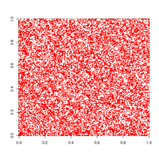
(b) The same graph, but with the vertices shuffled.

(c) Retrieving the clique in the shuffled graph

We will denote by $k=|S|$ the size of the hidden set. It is not hard to see that the problem is easy for $k$ large (both from the statistical and the computational point of view), and hard for $k$ small (both computationally and a statistically). Indeed, for $k$ sufficiently large, a simple degree based heuristics is successful. This is based on the remark that vertices in the clique have a slightly higher degree than others. Hence sorting the vertices by degree, the first $k$ vertices should provide a good estimate of $S$.

Proposition 1.

Let $\widehat{S}$ be the set of $k$ vertices with larges degree in $G$. If $k\geq\sqrt{(2+{\varepsilon})n\log n}$, then with high probability $\widehat{S}=S$.

Proof.

Let $D_{i}$ denote the degree of vertex $i$. If $i\not\in S$, then $D_{i}\sim{\rm Binom}(n-1,1/2)$. In particular, standard concentration bounds on independent random variables yield ${\mathbb{P}}\{D_{i}\geq{\mathbb{E}}D_{i}+t\}\leq\exp(-2t^{2}/n)$. By a union bound (the same already used to analyze denoising in Section 3.1), and using ${\mathbb{E}}(D_{i})=(n-1)/2$, we have, for any ${\varepsilon}^{\prime}>0$, with probability converging to one as $n\to\infty$,

$$\max_{i\not\in S}D_{i}\leq\frac{n}{2}+\sqrt{(1+{\varepsilon}^{\prime})\frac{n\log n}{2}}\,.$$ (142)

On the other hand, if $i\in S$, then $D_{i}\sim k-1+{\rm Binom}(n-k,1/2)$. Hence, by a similar union bound

$$\min_{i\in S}D_{i}\geq\frac{n+k}{2}-\sqrt{(1+{\varepsilon}^{\prime})\frac{n\log k}{2}}\,.$$ (143)

The claim follows by using together the above, and selecting a suitable value ${\varepsilon}^{\prime}$. ∎

For $k$ too small, the problem becomes statistically intractable because the planted clique is not the unique clique of size $k$. Hence no estimator can distinguish between the set $S$ and another set $S^{\prime}$ that supports a different (purely random) clique. The next theorem characterizes this statistical threshold.

Proposition 2.

Let ${\varepsilon}>0$ be fixed. Then, for $k<2(1-{\varepsilon})\log_{2}n$ any estimator $\widehat{S}$ is such that $\widehat{S}\neq S$ with probability converging to one as $n\to\infty$.

Viceversa, for $k<2(1-{\varepsilon})\log_{2}n$ there exists an estimator $\widehat{S}$ such that $\widehat{S}=S$ with probability converging to one as $n\to\infty$.

Proof.

We will not present a complete proof but only sketch the fundamental reason for a threshold $k\approx 2\log_{2}n$ and leave to the reader the task of filling the details.

The basic observation is that the largest ‘purely random’ clique is of size approximately $2\log_{2}n$. As a consequence, for $k$ larger than this threshold, searching for a clique of size $k$ returns the planted clique.

More precisely, let ${\mathcal{G}}(n,1/2)$ be an Erdös-Renyi random graph with edge density $1/2$ (i.e. a random graph where each edge is present independently with probability $1/2$). We will show that the largest clique in ${\mathcal{G}}(n,1/2)$ is with high probability of size between $2(1-{\varepsilon})\log_{2}n$ and $2(1+{\varepsilon})\log_{2}n$.

This claim can be proved by a moment calculation. In particular, for proving that the largest clique cannot be much larger than $2\log_{2}n$, it is sufficient to compute the expected number of cliques of size $\ell$. Letting $N(\ell;n)$ denote the number of cliques of size $\ell$ in ${\mathcal{G}}(n,1/2)$, we have

$${\mathbb{E}}\,N(\ell;n)=\binom{n}{\ell}2^{-\binom{\ell}{2}}\approx n^{\ell}2^{-\ell^{2}/2}=2^{\ell\log_{2}n-\ell^{2}/2}.$$ (144)

For $\ell>2(1+{\varepsilon})\log_{2}n$ the exponent is negative and the expectation vanishes as $n\to\infty$. In fact $\sum_{\ell\geq 2(1+{\varepsilon})\log_{2}n}{\mathbb{E}}N(\ell;n)$ vanishes as well. By Markov inequality, it follows that –with high probability– no clique has size larger than $2(1+{\varepsilon})\log_{2}n$. ∎

The catch with the last proposition is that the estimator needs not to be computable in polynomial time. Indeed the estimator implicitly assumed in the proof requires searching over all subsets of $k$ vertices, which takes time at least $\binom{n}{k}\approx n^{k}$. For $k$ above the threshold, this is $\exp\{c(\log n)^{2}\}$, that is super-polynomial.

To summarize, with unlimited computational resources we can find planted cliques as soon as their size is larger than $c\log_{2}n$ for any $c>2$. This is the fundamental statistical barrier towards estimating the set $S$/ On the other hand, the naive degree-based heuristic described above, correctly identifies the clique if $k\geq\sqrt{c\,n\log n}$. There is a huge gap between the fundamental statistical limit, and what is achieved by a simple polynomial-time algorithm. This begs the question as to whether this gap can be filled by more advanced algorithmic ideas.

A key observation, due to Alon, Krivelevich and Sudakov [59] is that the matrix ${\mathbf{W}}$ –in expectation– a rank-one matrix. Namely

$${\mathbb{E}}\{{\mathbf{W}}\}=u_{S}\,u_{S}^{sT}\,,$$ (145)

and therefore $S$ can be reconstructed from the eigenvalue decomposition of ${\mathbb{E}}\{{\mathbf{W}}\}$. Of course ${\mathbb{E}}\{{\mathbf{W}}\}$ is not available, but one can hope the random part of ${\mathbf{W}}$ not to perturb too much the leading eigenvector. In other words, one can compute the principal eigenvector $v_{1}({\mathbf{W}})$, i.e. the eigenvector of ${\mathbf{W}}$ with largest eigenvalue, and use its largest entries to estimate the clique. For instance, one can take the $k$ vertices corresponding to the entries of $v_{1}({\mathbf{W}})$ with largest absolute value.

This spectral approach allows to reduce the minimum detectable clique size by a factor $\sqrt{\log n}$, with respect to the degree heuristics of 1.

Theorem 3 (Alon, Krivelevich and Sudakov, 1998).

There exists an algorithm that returns an estimate $\widehat{S}$ of the set $S$, with the same complexity as computing the principal eigenvector of ${\mathbf{W}}$, and such that the following holds. If $k>100\sqrt{n}$, then $\widehat{S}=S$ with probability converging to one as $n\to\infty$.

Proof sketch.

Again, we will limit ourselves to explaining the basic argument. The actual proof requires some additional steps.

Then the matrix ${\mathbf{W}}$ has the form

$${\mathbf{W}}=u_{S}u_{S}^{{\sf T}}+{\bf Z}-{\bf Z}_{SS},$$ (146)

where ${\bf Z}$ is a Wigner matrix i.e. a matrix with i.i.d. zero-mean entries $({\bf Z}_{ij})_{i\leq j}$, and ${\bf Z}_{S,S}$ is the restriction of ${\bf Z}$ to indices in $S$. In the present case, the entries distribution is Bernoulli

$${\bf Z}_{ij}=\begin{cases}+1,&\text{with probability }1/2\\ -1,&\text{with probability }1/2\end{cases}.$$ (147)

By the celebrated Füredi-Komlos theorem of [60], the operator norm of this matrix (i.e. the maximum of the largest eigenvalue of ${\bf Z}$ and the largest eigenvalue of $-{\bf Z}$) is upper bounded as $\|{\bf Z}\|_{2}\leq(2+{\varepsilon})\sqrt{n}$, with high probability. By the same argument $\|{\bf Z}_{SS}\|_{2}\leq(2+{\varepsilon})\sqrt{k}$, which is much smaller than $\|{\bf Z}\|_{2}$.

We view ${\mathbf{W}}$ as a perturbation of the matrix $u_{S}u_{S}^{{\sf T}}$ (whose principal, normalized, eigenvector is $u_{S}/\sqrt{k}$). Matrix perturbation theory implies that the largest eigenvector is perturbed by an amount proportional to the norm of the perturbation and inversely proportional to the gap between top eigenvalue and second eigenvalue of the perturbed matrix. More precisely, Davis-Kahan ‘sin theta’ theorem yields (for $v_{1}=v_{1}({\mathbf{W}})$)

$$\sin\theta(v_{1},u_{S})\leq\frac{\|{\bf Z}-{\bf Z}_{S,S}\|_{2}}{\lambda_{1}(u_{S}u_{S}^{{\sf T}})-\lambda_{2}({\mathbf{W}})}\,,$$ (148)

where $\lambda_{\ell}({\mathbf{A}})$ denotes the $\ell$-th largest eigenvalue of matrix ${\mathbf{A}}$, and $\theta(a,b)$ is the angle between vectors $a$ and $b$. We of course have $\lambda_{1}(u_{S}u_{S}^{{\sf T}})=\|u_{S}\|_{2}^{2}=k$, and $\lambda_{2}({\mathbf{W}})\leq\lambda_{2}(u_{S}u_{S}^{{\sf T}})+\|{\bf Z}-{\bf Z}_{S,S}\|_{2}$. Therefore, for

$$\sin\theta(v_{1},u_{S}) \leq\frac{\|{\bf Z}-{\bf Z}_{S,S}\|_{2}}{k-\|{\bf Z}-{\bf Z}_{S,S}\|_{2}}$$ (149)

$$\leq\frac{2.1\sqrt{n}}{k-2.1\sqrt{n}}\leq frac{1}{45}\,.\,,$$ (150)

where the last inequality holds with high probability by Füredi-Komlos theorem. Using standard trigonometry, this bound can be immediately converted in a bound on the $\ell_{2}$ distance between $v_{1}({\mathbf{W}})$ and the unperturbed eigenvector:

$$\Big{\|}v_{1}-\frac{u_{S}}{\sqrt{k}}\Big{\|}_{2}\leq\frac{1}{40}\,.$$ (151)

We can then select the set $B$ of $k$ vertices that correspond to the $k$ entries of $v_{1}$ with largest absolute value. The last bound does not guarantee that $B$ coincide with $S$, but it implies that $B$ must have a substantial overlap with $S$. The estimator $\widehat{S}$ is constructed by selecting the $k$ vertices in $\{1,2,\dots,p\}$ that have the largest number of neighbors in $B$. ∎

It is useful to pause for a few remarks on this result.

Remark 1.

The complexity of the above algorithm is the same as the one of computing the principale eigenvector $v_{1}({\mathbf{W}})$. Under the assumptions of the theorem, this is non-degenerate and in fact, there is a large gap between the first eigenvalue and the second one, say $\max(\lambda_{2}({\mathbf{W}}),|\lambda_{n}({\mathbf{W}})|)\leq(1/2)\lambda_{1}({\mathbf{W}})$.

Hence, $v_{1}({\mathbf{W}})$ can be computed efficiently through power iteration, i.e. by computing the sequence of vectors $v^{(t+1)}={\mathbf{W}}v^{(t)}$. Each operation takes at most $n^{2}$ operations, and due to the fast convergence, $O(\log n)$ iterations are sufficient for implementing the above algorithm. We will revisit power iteration in the following.

Remark 2.

The eigenvalues and eigenvectors of a random matrix of the form (146) have been studied in detail in statistics (under the name of ‘spiked model’) and probability theory (as ‘low-rank perturbation of Wigner matrices’), see e.g. [61, 62, 63]. These work unveil a phase transition phenomenon that, in the present application, can be stated as follows. Assume $k,n\to\infty$ with $k/\sqrt{n}=\kappa\in(0,\infty)$. Then

$$\lim_{n\to\infty}|\langle v_{1}({\mathbf{W}}),u_{S}/\sqrt{k}\rangle|=\left\{\begin{array}[]{ll}0&\mbox{ if $\kappa\leq 1$,}\\ \sqrt{1-\kappa^{-2}}&\mbox{ otherwise.}\end{array}\right.$$ (154)

In other words, for $k\leq(1-{\varepsilon})\sqrt{n}$ the principal eigenvector of ${\mathbf{W}}$ is essentially uncorrelated with the hidden set $S$. The barrier at $k$ of order $\sqrt{n}$ is not a proof artifact, but instead a fundamental limit related to this phase transition.

On the other hand, a more careful analysis of the spectral method can possibly show that it succeeds for all $k\geq(1+{\varepsilon})\sqrt{n}$. (Here and above ${\varepsilon}>0$ is an arbitrary constant).

Remark 3.

A clever trick by Alon and collaborators [59], allow to find cliques of size $k\geq\delta\sqrt{n}$ for any fixed constant $\delta>0$ in polynomial time. The price to pay is that the computational complexity increases rapidly as $\delta$ gets smaller. ore precisely, we can identify sets of size $k\geq\delta\sqrt{n}$ for any with time complexity of order $n^{O(\log(1/\delta))}$.

To see this, we use the spectral method as a routine that is able to find the clique with high probability provided $k\geq c\sqrt{n}$ for some constant $c$. First assume that an oracle gives us one node in the clique. We can solve the problem with $k\gtrsim c\sqrt{n/2}$. Indeed we can focus our attention on the set of neighbors of the node provided by the oracle. There is about $n/2$ such neighbors, and they contain a clique of size $k-1$, hence the spectral method will succeed under the stated condition.

We then observe that we do not need an such: we can search for the vertex that the oracle would tell us by blowing up the runtime by a factor at most $n$ (indeed only a $\sqrt{n}$ factor is sufficient, since one every $\sqrt{n}$ vertices is in the clique). In this way we can trade a factor of $\sqrt{2}$ in $k$ by an $n$-fold increase of the runtime. This construction can be repeated $O(\log(1/\delta))$ times to achieve the trade-off mentioned above.

6.1. An iterative thresholding approach

Throughout this section, we shall normalize the data and work with the matrix ${\mathbf{A}}={\mathbf{W}}/\sqrt{n}$. As we saw in the previous section, the principal eigenvector of ${\mathbf{A}}$ carries important information about the set $S$, and in particular it is correlated with the indicator vector $u_{S}$, if the hidden set $S$ is large enough. Also an efficient way to compute the principal eigenvector is through power iteration

$$v^{(t+1)}={\mathbf{A}}\,v^{(t)}\,.$$ (155)

Note that the resulting vector $v^{(t)}$ will not –in general– be sparse, if not, a posteriori, because of the correlation with $u_{S}$. It is therefore a natural idea to modify the power iteration by introducing a non-linearity that enforces sparsity:

$$\theta^{(t+1)}={\mathbf{A}}\,f_{t}(\theta^{(t)}),$$ (156)

where $\theta\in^{n}$ and $f_{t}:^{n}\to^{n}$ is a non-linear function that enforces sparsity. To be definite, we will assume throughout that the initialization is $\theta^{(0)}=(1,1,\dots,1)$, the all-ones vector.

For ease of exposition, we shall focus on separable functions and denote by $f_{t}$ the action of this function on each component. In other words, with a slight abuse of notation, we will write $f_{t}(v)=(f_{t}(v_{1}),f_{t}(v_{2}),\dots,f_{t}(v_{n}))$ when $v=(v_{1},v_{2},\dots,v_{n})$. Example of such a function might be

• Positive soft thresholding: $f_{t}(x)=(x-\lambda_{t})_{+}$ for some iteration-dependent threshold $\lambda_{t}$. The threshold can be chosen so that, on average $f_{t}(\theta^{(t)})$ has a number of non-zeros of order $k$.

• Positive hard thresholding: $f_{t}(x)=x\,{\mathbb{I}}(x\geq\lambda_{t})$ (here ${\mathbb{I}}$ is the indicator function: ${\mathbb{I}}(B)=1$ if $B$ is true and $=0$ otherwise). Again $\lambda_{t}$ is a threshold.

• Logistic nonlinearity:

  $$f_{t}(x)=\frac{1}{1+\exp(-a_{t}(x-\lambda_{t}))}\,,$$ (157)

  where $\lambda_{t}$ plays the role of a ‘soft threshold.’

Which function should we choose? Which thresholds? Will this approach beat the simple power iteration (i.e. $f_{t}(x)=x$)?

In order to address these questions, we will carry out a simple heuristic analysis of the above non-linear power iteration. Remarkably, we will see in the next section that this analysis yields the correct answer for a modified version of the same algorithm –a message passing algorithms. Our discussion is based on [58], and we refer to that paper for al omitted details, formal statements and derivations.

The heuristic analysis requires to consider separately vertices in $S$ and outside $S$:

1. For $i\not\in S$, the non-linear power iteration (156) reads

   $$\theta_{i}^{(t+1)}=\sum_{j=1}^{n}{\mathbf{A}}_{ij}f_{t}(\theta_{j}^{(t)})\,.$$ (158)

   Since in this case the variables $\{{\mathbf{A}}_{ij}\}_{j\in[n]}$ are i.i.d. with mean zero and variance $1/n$, it is natural to guess –by central limit theorem– $\theta_{i}^{(t+1)}$ to be approximately normal with mean $0$ and variance $(1/n)\sum_{j=1}^{n}f_{t}^{2}(\theta_{j}^{(t)})$. Repeating this argument inductively, we conclude that that $\theta_{i}^{t}\sim\mathcal{N}\left(0,\sigma_{t}^{2}\right)$, where –by the law of large numbers applied to $(1/n)\sum_{j=1}^{n}f_{t}^{2}(\theta_{j}^{(t)})$–

   $$\sigma_{t+1}^{2}={\mathbb{E}}\big{\{}f_{t}(\sigma_{t}\,Z)^{2}\big{\}}\,,$$ (159)

   where the expectation is taken with respect to $Z\sim\mathcal{N}\left(0,1\right)$. The initialization $\theta^{(0)}=u$ implies $\sigma_{1}^{2}=f_{0}(1)^{2}$

2. For $i\in S$, we have ${\mathbf{A}}_{ij}=\kappa$ if $j\in S$ as well, and ${\mathbf{A}}_{ij}={\bf Z}_{ij}/\sqrt{n}$ having zero mean and variance $1/n$ otherwise. Hence

   $$\theta_{i}^{(t+1)}=\kappa\sum_{j\in S}f_{t}(\theta_{j}^{(t)})+\frac{1}{\sqrt{n}}\sum_{j\in[n]\setminus S}{\bf Z}_{ij}f_{t}(\theta_{j}^{(t)})\,.$$ (160)

   By the same argument as above, the second part gives rise to a zero-mean Gaussian contribution, with variance $\sigma_{t}^{2}$, and the first has non-zero mean and negligible variance. We conclude that $\theta_{i}^{(t)}$ is approximately $\mathcal{N}\left(\mu_{t},\sigma_{t}^{2}\right)$ with $\sigma_{t}$ given recursively by Eq. (159). Applying the law of large numbers to the non-zero mean contribution, we get the recursion

   $$\mu_{t+1}=\kappa\,{\mathbb{E}}\big{\{}f_{t}(\mu_{t}+\sigma_{t}\,Z)\big{\}}\,,$$ (161)

   where the expectation is taken with respect to $Z\sim\mathcal{N}\left(0,1\right)$, and the initialization $\theta^{(0)}=u$ implies $\mu_{1}=\kappa\,f_{0}(1)$ (recall that $\kappa$ is defined as the limit of $k/\sqrt{n}$.

A few important remarks.

The above derivation is of course incorrect! The problem is that the central limit theorem cannot be applied to the right-hand side of Eq. (158) because the summands are not independent. Indeed, each term $f_{t}(\theta^{(t)}_{j})$ depends on all the entries of the matrix ${\mathbf{A}}$.

The conclusion that we reached is incorrect. It is not true that, asymptotically, $\theta^{(t)}_{i}$ is approximately Gaussian, with the above mean and variance.

Surprisingly, the conclusion is correct for a slightly modified algorithm, namely a message passing algorithm that will be introduced in the next section. This is a highly non-trivial phenomenon

6.2. A message passing algorithm

We modify the non-linear power iteration (158) by transforming it into a message passing algorithm, whose underlying graph is the complete graph with $n$ vertices. The iteration variables are ‘messages’ $\theta^{(t)}_{i\to j}$ for each $i\neq j$ (with $\theta^{(t)}_{i\to j}\neq\theta^{(t)}_{j\to i}$. These are updated using the rule

$$\theta_{i\to j}^{(t)}=\sum_{k\in[n]\setminus j}{\mathbf{A}}_{ik}f_{t}(\theta_{k\to i}^{(t)})\,.$$ (162)

The only difference with respect to the iteration (158) is that we exclude the term $k=j$ from the sum. Despite this seemingly negligible change (one out of $n$ terms is dropped), the statistical properties of this algorithm are significantly different from the ones of the nonlinear power iteration (158), even in the limit $n\to\infty$. In particular, the Gaussian limit derived heuristically in the previous section, holds for the message passing algorithm. Informally, we have, as $n\to\infty$,

$$\theta_{i\to j}^{(t)}\sim\begin{cases}\mathcal{N}\left(\mu_{t},\sigma_{t}^{2}\right)&\mbox{ if $i\in S$},\\ \mathcal{N}\left(0,\sigma_{t}^{2}\right)&\mbox{ if $i\not\in S$},\end{cases}$$ (163)

where $\mu_{t},\sigma_{t}$ are determined by the state evolution equations (159) and (159).

Let us stress that we did not yet choose the functions $f_{t}(\,\cdot\,)$: we defer this choice, as well as an analysis of state evolution to the next section. Before this, we note that –as in the case of sparse regression– an approximate message passing (AMP) version of this algorithm can be derived by writing $\theta^{(t)}_{i\to j}=\theta^{(t)}_{i}+\delta\theta^{(t)}_{i\to j}$ and linearizing in the latter correction. This calculation leads to the simple AMP iteration

$$\theta^{(t+1}={\mathbf{A}}f_{t}(\theta^{(t)})-{\sf b}_{t}f_{t-1}(\theta^{(t-1)}),$$ (164)

where the ‘Onsager term’ ${\sf b}_{t}$ is given in this case by

$${\sf b}_{t}=\frac{1}{n}\sum_{i=1}^{n}f^{\prime}_{t}(\theta^{(t)}_{i})\,.$$ (165)

6.3. Analysis and optimal choice of $f_{t}(\,\cdot\,)$

We now consider the implications of state evolution for the performance of the above message passing algorithms. For the sake of simplicity, we will refer to the AMP form (164), but analogous statements hold for the message passing version (162). Informally, state evolution implies that

$$\theta^{(t)}\approx\mu_{t}\,u_{S}+\sigma_{t}\,z\,,$$ (166)

where $z\sim\mathcal{N}\left(0,{\rm I}_{n}\right)$, and this statement holds asymptotically in the sense of finite-dimensional marginals.

In other words, we can interpret $\theta^{(t)}$ as a noisy observation of the unknown vector $u_{S}$, corrupted by Gaussian noise. This suggest to choose $f_{t}(\,\cdot\,)$ as the posterior expectation denoiser. Namely, for $y\in$

$$f^{{\rm opt}}_{t}(y)={\mathbb{E}}\{U|\,\mu_{t}\,U+\sigma_{t}\,Z=y\big{\}}\,,$$ (167)

where $U\sim{\rm Bernoulli}(p)$ for $p=k/n=\kappa/\sqrt{n}$, and $Z\sim\mathcal{N}\left(0,1\right)$ independently of $U$. A simple calculation yields the explicit expression

$$f^{{\rm opt}}_{t}(y)=\frac{\delta}{\delta+(1-\delta)\,\exp\Big{(}-\frac{\mu_{t}}{\sigma_{t}^{2}}y+\frac{\mu_{t}^{2}}{\sigma_{t}^{2}}\Big{)}}\,.$$ (168)

This is indeed empirically the best choice for the non-linearity $f^{{\rm opt}}_{t}(\,\cdot\,)$. We shall next rederive it from a different point of view, which also allow to characterize its behavior.

Reconsider again the Gaussian limit (166). It is clear that the quality of the information contained in $\theta^{(t)}$ depends on signal to noise ratio $\mu_{t}/\sigma_{t}$. Note that $u_{S}$ is very sparse, hence the vector $\theta^{(t)}$ is undistinguishable from a zero-mean Gaussian vector unless $(\mu_{t}/\sigma_{t})\to\infty$. Indeed, unless this happens, the entries $\theta^{(t)}_{i}$, $i\in S$, are hidden in the tail of the zero-mean entries $\theta^{(t)}_{i}$, $i\in[n]\setminus S$, see figure below. It turns out that, by optimally choosing $f_{t}(\,\cdot\,)$, this happens if and only if $\kappa>1/\sqrt{e}$. In other words, the message passing algorithm succeeds with high probability as long as $k$ is larger than $(1+{\varepsilon})\sqrt{n/e}$, for any ${\varepsilon}>0$.

In order to determine the whether $\widetilde{\mu}_{t}\equiv(\mu_{t}/\sigma_{t})\to\infty$, note that –without loss of generality– we can rescale the functions $f_{t}(\,\cdot\,)$ so that $\sigma_{t}=1$ for all $t$ (simply replacing $f_{t}(z)$ by $f_{t}(z)/{\mathbb{E}}\{f_{t}(Z)^{2}\}^{1/2}$ in Eq. (162), or in Eq. (164)). After this normalization, Eq. (161) yields

$$\widetilde{\mu}_{t+1}=\kappa\frac{{\mathbb{E}}\left\{f_{t}(\widetilde{\mu}_{t}+Z)\right\}}{{\mathbb{E}}\{f_{t}(Z)^{2}\}^{1/2}}\ .$$ (169)

Note that

$${\mathbb{E}}\left\{f_{t}(\widetilde{\mu}_{t}+Z)\right\} =\int f_{t}(x)\,\frac{1}{\sqrt{2\pi}}\,e^{-(x-\mu_{t})^{2}/2}\,{\rm d}x$$ (170)

$$=e^{-\widetilde{\mu}_{t}^{2}/2}{\mathbb{E}}\big{\{}f_{t}(Z)\,e^{\widetilde{\mu}_{t}x}\big{\}}\leq e^{\widetilde{\mu}_{t}^{2}}{\mathbb{E}}\big{\{}f_{t}(Z)^{2}\big{\}}^{1/2}\,.$$ (171)

where the last inequality follows from Cauchy-Schwartz inequality. The inequality is saturated by taking $f_{t}(x)=e^{\widetilde{\mu}_{t}x-(\widetilde{\mu}_{t}^{2}/2)}$, that yields the state evolution recursion

$$\widetilde{\mu}_{t+1}=\kappa\,e^{\widetilde{\mu}_{t}^{2}/2}\,.$$ (172)

It is immediate to study this recursion, and conclude that $\widetilde{\mu}_{t}\to\infty$ if and only if $\kappa>1/\sqrt{e}$.

The above analysis indeed yields the correct threshold for a message passing algorithm, as proved in [58]. (For proving the theorem below, a ‘cleaning’ step is added to the message passing algorithm.)

Theorem 4 (Deshpande, Montanari, 2014).

There exists an algorithm with time complexity $O(n^{2}\log n)$, that outputs an estimate $\widehat{S}$ such that –if $k>(1+\epsilon)\sqrt{\frac{n}{e}}$– then $\widehat{S}=S$ with probability converging to one as $n\to\infty$.

In other words, the message passing algorithm is able to find cliques smaller by a factor $1/\sqrt{e}$ with respect to spectral methods, with no increase in complexity. A natural research question is the following:

Is it possible to planted find cliques of size $(1-{\varepsilon})\sqrt{n/e}$ in time $O(n^{2}\log n)$?

The paper [58] provides a partially positive answer to this question, by showing that no ‘local algorithm’ (a special class of linear-time algorithm) can beat message passing algorithms for a sparse-graph version of the planted clique problem.

Let us conclude by showing how the last derivation agrees in fact with the guess (168) for the optimal non-linearity. Note that $\delta=\kappa/\sqrt{n}\to 0$ as $n\to\infty$. In this limit

$$f^{{\rm opt}}_{t}(y)\approx C_{t}\,\exp\Big{\{}\frac{\mu_{t}}{\sigma_{t}^{2}}\,y\Big{\}}\,.$$ (173)

This coincides with the choice optimizing the state evolution threshold, once we set $\sigma_{t}=1$ (that entails no loss of generality).

References

- [1] L. Wasserman, All of statistics: a concise course in statistical inference. Springer, 2004.
- [2] ——, All of nonparametric statistics. Springer, 2006.
- [3] I. M. Johnstone, Gaussian estimation: Sequence and wavelet models, 2011, draft version, December 27, 2011, available at http://statweb.stanford.edu/ imj/GE12-27-11.pdf.
- [4] A. B. Tsybakov and V. Zaiats, Introduction to nonparametric estimation. Springer, 2009, vol. 11.
- [5] P. Bühlmann and S. Van De Geer, Statistics for high-dimensional data: methods, theory and applications. Springer, 2011.
- [6] F. J. Herrmann, M. P. Friedlander, and Ö. Yilmaz, “Fighting the curse of dimensionality: Compressive sensing in exploration seismology,” Signal Processing Magazine, vol. 29, no. 3, pp. 88–100, 2012.
- [7] D. Donoho, I. Johnstone, and A. Montanari, “Accurate prediction of phase transitions in compressed sensing via a connection to minimax denoising,” Information Theory, IEEE Transactions on, vol. 59, no. 6, pp. 3396–3433, June 2013.
- [8] C. F. Gauss, Theoria combinationis observationum erroribus minimis obnoxiae. H. Dieterich, 1823.
- [9] W. James and C. Stein, “Estimation with quadratic loss,” in Proceedings of the fourth Berkeley symposium on mathematical statistics and probability, vol. 1, no. 1961, 1961, pp. 361–379.
- [10] D. L. Donoho and I. M. Johnstone, “Minimax risk over balls,” Prob. Th. and Rel. Fields, vol. 99, pp. 277–303, 1994.
- [11] ——, “Neo-classical minimax problems, thresholding, and adaptation,” Bernoulli, pp. 39–62, 1994.
- [12] D. Donoho and I. Johnstone, “Adapting to unknown smoothness via wavelet shrinkage,” J. Amer. Statist. Assn., vol. 90, pp. 1200–1224, 1995.
- [13] D. L. Donoho and I. M. Johnstone, “Minimax estimation via wavelet shrinkage,” Annals of Statistics, vol. 26, pp. 879–921, 1998.
- [14] B. Derrida, “Random-energy model: An exactly solvable model of disordered systems,” Physical Review B, vol. 24, no. 5, p. 2613, 1981.
- [15] D. L. Donoho and J. M. Johnstone, “Ideal spatial adaptation by wavelet shrinkage,” Biometrika, vol. 81, no. 3, pp. 425–455, 1994.
- [16] D. L. Donoho, A. Maleki, and A. Montanari, “Message-passing algorithms for compressed sensing,” Proceedings of the National Academy of Sciences, vol. 106, no. 45, pp. 18 914–18 919, 2009.
- [17] ——, “The noise-sensitivity phase transition in compressed sensing,” Information Theory, IEEE Transactions on, vol. 57, no. 10, pp. 6920–6941, 2011.
- [18] R. Tibshirani, “Regression shrinkage and selection with the Lasso,” J. Royal. Statist. Soc B, vol. 58, pp. 267–288, 1996.
- [19] S. Chen and D. Donoho, “Examples of basis pursuit,” in Proceedings of Wavelet Applications in Signal and Image Processing III, San Diego, CA, 1995.
- [20] S. S. Chen, D. L. Donoho, and M. A. Saunders, “Atomic decomposition by basis pursuit,” SIAM journal on scientific computing, vol. 20, no. 1, pp. 33–61, 1998.
- [21] A. Juditsky and A. Nemirovski, “First order methods for nonsmooth convex large-scale optimization,” Optimization for Machine Learning, pp. 121–148, 2011.
- [22] I. Daubechies, M. Defrise, and C. De Mol, “An iterative thresholding algorithm for linear inverse problems with a sparsity constraint,” Communications on pure and applied mathematics, vol. 57, no. 11, pp. 1413–1457, 2004.
- [23] A. Beck and M. Teboulle, “A fast iterative shrinkage-thresholding algorithm for linear inverse problems,” SIAM Journal on Imaging Sciences, vol. 2, no. 1, pp. 183–202, 2009.
- [24] E. J. Candés and T. Tao, “Decoding by linear programming,” IEEE Trans. on Inform. Theory, vol. 51, pp. 4203–4215, 2005.
- [25] E. Candés and T. Tao, “The dantzig selector: Statistical estimation when p is much larger than n,” The Annals of Statistics, pp. 2313–2351, 2007.
- [26] P. J. Bickel, Y. Ritov, and A. B. Tsybakov, “Simultaneous analysis of Lasso and Dantzig selector,” Amer. J. of Mathematics, vol. 37, pp. 1705–1732, 2009.
- [27] M. Rudelson and R. Vershynin, “On sparse reconstruction from fourier and gaussian measurements,” Communications on Pure and Applied Mathematics, vol. 61, no. 8, pp. 1025–1045, 2008.
- [28] J. A. Tropp, J. N. Laska, M. F. Duarte, J. K. Romberg, and R. G. Baraniuk, “Beyond nyquist: Efficient sampling of sparse bandlimited signals,” Information Theory, IEEE Transactions on, vol. 56, no. 1, pp. 520–544, 2010.
- [29] D. L. Donoho, “High-dimensional centrally symmetric polytopes with neighborliness proportional to dimension,” Discrete & Computational Geometry, vol. 35, no. 4, pp. 617–652, 2006.
- [30] D. L. Donoho and J. Tanner, “Neighborliness of randomly projected simplices in high dimensions,” Proceedings of the National Academy of Sciences of the United States of America, vol. 102, no. 27, pp. 9452–9457, 2005.
- [31] ——, “Sparse nonnegative solution of underdetermined linear equations by linear programming,” Proceedings of the National Academy of Sciences of the United States of America, vol. 102, no. 27, pp. 9446–9451, 2005.
- [32] V. Chandrasekaran, B. Recht, P. A. Parrilo, and A. S. Willsky, “The convex geometry of linear inverse problems,” Foundations of Computational Mathematics, vol. 12, no. 6, pp. 805–849, 2012.
- [33] E. Candés and B. Recht, “Simple bounds for recovering low-complexity models,” Mathematical Programming, vol. 141, no. 1-2, pp. 577–589, 2013.
- [34] M. Stojnic, “A framework to characterize performance of lasso algorithms,” arXiv preprint arXiv:1303.7291, 2013.
- [35] S. Oymak, C. Thrampoulidis, and B. Hassibi, “The squared-error of generalized lasso: A precise analysis,” arXiv preprint arXiv:1311.0830, 2013.
- [36] D. Amelunxen, M. Lotz, M. B. McCoy, and J. A. Tropp, “Living on the edge: A geometric theory of phase transitions in convex optimization,” arXiv preprint arXiv:1303.6672, 2013.
- [37] Y. Kabashima, T. Wadayama, and T. Tanaka, “A typical reconstruction limit for compressed sensing based on lp-norm minimization,” Journal of Statistical Mechanics: Theory and Experiment, vol. 2009, no. 09, p. L09003, 2009.
- [38] S. Rangan, V. Goyal, and A. K. Fletcher, “Asymptotic analysis of map estimation via the replica method and compressed sensing,” in Advances in Neural Information Processing Systems, 2009, pp. 1545–1553.
- [39] D. Guo, D. Baron, and S. Shamai, “A single-letter characterization of optimal noisy compressed sensing,” in Communication, Control, and Computing, 2009. Allerton 2009. 47th Annual Allerton Conference on. IEEE, 2009, pp. 52–59.
- [40] F. Krzakala, M. Mézard, F. Sausset, Y. Sun, and L. Zdeborová, “Statistical-physics-based reconstruction in compressed sensing,” Physical Review X, vol. 2, no. 2, p. 021005, 2012.
- [41] M. Bayati and A. Montanari, “The dynamics of message passing on dense graphs, with applications to compressed sensing,” Information Theory, IEEE Transactions on, vol. 57, no. 2, pp. 764–785, 2011.
- [42] ——, “The lasso risk for gaussian matrices,” Information Theory, IEEE Transactions on, vol. 58, no. 4, pp. 1997–2017, 2012.
- [43] A. Javanmard and A. Montanari, “State evolution for general approximate message passing algorithms, with applications to spatial coupling,” Information and Inference, p. iat004, 2013.
- [44] D. Donoho, A. Javanmard, and A. Montanari, “Information-theoretically optimal compressed sensing via spatial coupling and approximate message passing,” Information Theory, IEEE Transactions on, vol. 59, no. 11, pp. 7434–7464, Nov 2013.
- [45] M. Bayati, M. Lelarge, and A. Montanari, “Universality in polytope phase transitions and message passing algorithms,” Annals of Applied Probability, 2014.
- [46] D. L. Donoho, A. Maleki, and A. Montanari, “Message passing algorithms for compressed sensing: I. motivation and construction,” in Information Theory Workshop (ITW), 2010 IEEE. IEEE, 2010, pp. 1–5.
- [47] T. Richardson and R. Urbanke, Modern coding theory. Cambridge University Press, 2008.
- [48] M. Mezard and A. Montanari, Information, physics, and computation. Oxford University Press, 2009.
- [49] S. Som and P. Schniter, “Compressive imaging using approximate message passing and a markov-tree prior,” Signal Processing, IEEE Transactions on, vol. 60, no. 7, pp. 3439–3448, 2012.
- [50] S. Rangan, “Generalized Approximate Message Passing for Estimation with Random Linear Mixing,” in IEEE Intl. Symp. on Inform. Theory, St. Petersbourg, Aug. 2011, pp. 2168 – 2172.
- [51] D. Donoho and A. Montanari, “High dimensional robust m-estimation: Asymptotic variance via approximate message passing,” arXiv preprint arXiv:1310.7320, 2013.
- [52] C. A. Metzler, A. Maleki, and R. G. Baraniuk, “From denoising to compressed sensing,” arXiv preprint arXiv:1406.4175, 2014.
- [53] J. Tan, Y. Ma, and D. Baron, “Compressive imaging via approximate message passing with image denoising,” arXiv preprint arXiv:1405.4429, 2014.
- [54] J. Barbier and F. Krzakala, “Replica analysis and approximate message passing decoder for superposition codes,” arXiv preprint arXiv:1403.8024, 2014.
- [55] E. Bolthausen, “An iterative construction of solutions of the tap equations for the sherrington–kirkpatrick model,” Communications in Mathematical Physics, vol. 325, no. 1, pp. 333–366, 2014.
- [56] Q. Berthet and P. Rigollet, “Complexity theoretic lower bounds for sparse principal component detection,” in Conference on Learning Theory, 2013, pp. 1046–1066.
- [57] M. Jerrum, “Large cliques elude the metropolis process,” Random Structures & Algorithms, vol. 3, no. 4, pp. 347–359, 1992.
- [58] Y. Deshpande and A. Montanari, “Finding Hidden Cliques of Size in Nearly Linear Time,” arXiv:1304.7047, 2013.
- [59] N. Alon, M. Krivelevich, and B. Sudakov, “Finding a large hidden clique in a random graph,” in Proceedings of the ninth annual ACM-SIAM symposium on Discrete algorithms. Society for Industrial and Applied Mathematics, 1998, pp. 594–598.
- [60] Z. Füredi and J. Komlós, “The eigenvalues of random symmetric matrices,” Combinatorica, vol. 1, no. 3, pp. 233–241, 1981.
- [61] D. Féral and S. Péché, “The largest eigenvalue of rank one deformation of large wigner matrices,” Communications in mathematical physics, vol. 272, no. 1, pp. 185–228, 2007.
- [62] M. Capitaine, C. Donati-Martin, and D. Féral, “The largest eigenvalues of finite rank deformation of large wigner matrices: convergence and nonuniversality of the fluctuations,” The Annals of Probability, vol. 37, no. 1, pp. 1–47, 2009.
- [63] ——, “Central limit theorems for eigenvalues of deformations of wigner matrices,” in Annales de l’Institut Henri Poincaré, Probabilités et Statistiques, vol. 48, no. 1. Institut Henri Poincaré, 2012, pp. 107–133.