Evolution of single B-type stars
with a large angular momentum content

Abstract

Context. The Geneva Stellar Evolution Group has recently presented an extended database of rotating stellar models at three different metallicities for nine different initial rotation parameters and ten different masses corresponding to spectral types from early- F to late- O. With these grids we have contributed to the understanding of the evolution of single rotating stars, and we intend to use them to produce synthetic stellar populations that fully account for the effects of stellar rotation. However, up to now we still lacked stellar evolutionary tracks that rotate close to the critical limit during the whole main-sequence (MS) phase. This occurs because the flat internal profile of rotation imposed at the zero-age main sequence (ZAMS) is modified by the action of meridional currents immediately after the ZAMS, causing the surface rotational velocity to decrease abruptly until it reaches a quasi-stationary state.

Aims. We compute stellar models with non-solid rotation at the ZAMS, which allows us to obtain stellar evolutionary tracks with a larger content of angular momentum that rotate close to the breakup limit throughout the whole MS.

Methods. We produced stellar models by removing the assumption that stars rotate as solid bodies at the ZAMS. We obtained the stellar structure at the ZAMS with a differentially rotating profile for three different metallicities by performing pre-MS calculations and by proposing ad hoc initial rotational profiles. We then computed the MS evolution and later phases of stellar evolution of these models, which attain rotational equatorial velocities close to the critical limit throughout their whole MS phase.

Results. Stellar models with solid rotation at the ZAMS adequately represent the overall characteristics and evolution of differentially rotating models of identical angular momentum content, but with a lower initial surface rotational velocity rate, at Z=0.014, Z=0.006, and Z=0.002. For models with solid rotation at the ZAMS we therefore recommend to use as the initial rotational rate the values derived once the quasi-stationary state is reached, that is, after the abrupt decrease in surface velocity. By producing stellar structures at the ZAMS with differentially rotating profiles and larger angular momentum content than in our previous works, we obtain models that rotate close to the critical limit throughout the whole main sequence. These models have a longer MS lifetime and a higher surface chemical enrichment already at the end of the MS, particularly at Z=0.002. Interestingly, the initial equatorial rotational velocities are virtually metallicity independent for all stellar models we computed in the B-type star range with the same mass and angular momentum content at the ZAMS. If, as some observational evidence indicates, B-type stars at Z=0.002 rotate with a higher equatorial velocity at the ZAMS than stars with Z=0.014, our finding would indicate that the angular momentum content of B-type stars in the SMC is higher than their Galactic counterparts.

1 Introduction

Rotation has proved to play a relevant role on the formation, evolution, and the ultimate fate of stars (see e.g. Maeder, 2009) and, as a consequence, it has deep implications for the behaviour of different populations of stars in clusters and galaxies. Therefore, it is important to study rotating stellar populations to gain a better understanding of the physics of rotation in stars. To do this, it is necessary to explore, both from a theoretical and an observational point of view, groups of stars in which the effects of rotation are strong. In particular, the domain of B-type stars has been known for a long time to offer an exceptional laboratory for studying stellar rotation (Slettebak, 1966; Sackmann & Anand, 1970)[e.g.], because it hosts the largest portion of rapidly rotating stars. Among them, we find Be stars (see Rivinius et al., 2013, for a recent review on these rapidly rotating objects).

With the aim of studying in detail the effects of rotation troughout the B-type stellar range, Georgy et al. (2013) presented an extended database of models of rotating stars at three different metallicities for nine different initial rotation parameters and ten different masses (between 1.7 and 15 M_☉) at the zero-age main sequence (ZAMS). This was achieved by the numerous improvements that were implemented in the Geneva stellar evolution code (Ekström et al., 2012), which enable computing models of rotating stars, even those that rotate at the critical limit and experience episodes of mechanical mass loss (Georgy et al., 2013; Granada et al., 2013).

It is important to to keep in mind that in order to do this, many assumptions and simplifications were made, that enabled us to account for physical processes that are not unidimensional, such as rotation itself, convection, turbulent mixing, stellar winds, etc. Many of these processes are still poorly understood and remain treated with simple parametrized approximations. That is the case, for instance, of the choice of an overshooting parameter in convective regions, calibrated to ensure an adequate reproduction of the width of the MS sequence band in the Hertzprung-Russell diagram (HRD), or the prescription used for the diffusion coefficients that express the transport of angular momentum in rotating models, among others.

To improve the prescriptions we can benefit from 2D/3D models, which provide a more realistic description of the structure of rotating stars. For instance, Espinosa Lara & Rieutord (2011) have succedeed in obtaining a better description of the latitude dependency of the temperature in rapidly rotating stars. Other authors (e.g. Deupree et al., 2012) have calculated frequency spectra for rotating pulsators, which is useful to interpret the asteroseismic data. These types of data are most promising to set contraints on the internal structure of the star and its rotational properties and evolution (Eggenberger et al., 2012; Neiner et al., 2012). Multidimensional hydrodynamical simulations can als provide constraints on the treatment of turbulence (Arnett & Meakin, 2011) and hence better describe the transport of angular momentum inside the star. Until many of the new constraints prove to be better than the existing ones, we continue to use the same prescriptions that have been used in previous computations with the Geneva stellar evolution code.

We recall some of the main assumptions made for computing grids of rotating models.

• Shellular rotation hypothesis: $\Omega$ is constant on isobars, because of strong horizontal turbulence (Zahn, 1992). Under this assumption, there is no latitude dependency of stellar rotation.

• The shape of a rotating star is given by the Roche model, which assumes a central condensation of the stellar mass. In this framework, the surface of the star only depends on $\omega=\Omega/\Omega_{\rm crit}$, with $\Omega$ the angular velocity of the stellar surface and $\Omega_{\rm crit}$ the breakup angular velocity. Even for stars with a large angular momentum content such as those we present here the stellar interior rotates well below its critical limit, while the surface of the star is rotationally distorted, and 1D models remain an acceptable approximation.

• Because of the Von Zeipel effect, the stellar winds are anisotropic. In our computations we used the prescripions described by Georgy et al. (2011).

• Throughout the evolution of a rapidly rotating star, the equatorial rotational velocity can reach the break-up limit. In our models, we assume that stars reaching the critical limit will undergo mechanical mass and angular momentum losses, which we model as removing the overcritical layers of the star. However, the details of mechanical mass removal close to the critical limit are still not understood, and our models also lack the physical process to effectively push the matter outwards.

We refer to Ekström et al. (2008, 2012) and Georgy et al. (2013, 2011) for extensive explanations and details of the physical processes and assumptions made in our calculations.

We plan to use our rotating grids to produce synthetic populations of stars and study their evolution in time, fully accounting for mass, rotation and metallicity distributions, with our new population synthesis code (Georgy et al., 2014). The stellar models of the database were computed assuming solid-body rotation at the ZAMS, with the underlying assumption that pre- main sequence (pre-MS) stars are fully convective, similarly to the work by Heger et al. (2000), and assuming that convection drives rigid-body rotation. In our models, the action of meridional currents modifies the flat internal rotation profile just after the ZAMS when the solid-body constraint is released, which leads to a strong decrease of the surface rotation. In this scenario, our models therefore begin their evolution with a slow-down of their surface rotational velocity. If the initial velocity is high enough, they can reach the critical limit after some evolution on the main sequence (MS). As a consequence, the initial conditions of the calculations prevent obtaining very rapidly rotating stars at very young ages, even when imposing a high value of $\omega_{ini}$. Because we intend to study the evolution of rapidly rotating stellar populations, it is certainly a problem that we are unable to produce rapidly rotating stars from the ZAMS because of the strong assumption of an initial flat rotating profile.

The recent work by Haemmerlé et al. (2013), who computed models of pre-MS stellar evolution, can help us solve this problem. On the one hand, it allows us to study the validity of the assumption of solid-body rotation at the ZAMS, that is, to understand how stars with the same mass, metallicity and angular momentum content but different internal rotation profile at the ZAMS evolve. On the other hand, it permits us to produce very rapidly rotating stellar models from the ZAMS and throughout the whole MS lifetime.

Throughout the present article we extend and complement the work by Georgy et al. (2013). In Section 2 we describe the assumptions made by Haemmerlé et al. (2013) to obtain the internal rotation profile at the ZAMS, and describe the results obtained by these authors, which are relevant to the present work. Because we present here models with different metallicities, we also show that the results obtained for Z=0.014 are valid for lower metallicities as well. In Section 3 we present our new models of rapidly rotating stars from the ZAMS with a large angular momentum content, we describe their main characteristics, and show how they compare with the grids presented by Georgy et al. (2013). We conclude in Section 4.

2 Relevance of the internal rotational profile of a star at the ZAMS for its subsequent evolution

Haemmerlé et al. (2013) showed that stars that form through different pre-MS accretion prescriptions, but have the same content of total angular momentum at the ZAMS, follow the same subsequent evolution in terms of evolutionary tracks, surface velocities, and abundances, independently of their formation history. These authors computed pre-MS tracks for stars between 2 and 22 M_☉ at solar metallicity, using the Geneva stellar evolution code (Eggenberger et al., 2008; Ekström et al., 2012), including shellular rotation, and following different scenarios, with accretion or at constant mass. The initial model, at the top of the Hayashi line, is fully convective, and solid-body rotation is assumed in convective zones. During pre-MS evolution, large regions of the star become progressively radiative and a gradient of internal angular rotation velocity ($\Omega$) develops, so that the rotation profile obtained when the star reaches the ZAMS is not flat. For models reaching $\rm v_{surf}/v_{crit}=0.4$ on the ZAMS in the accretion scenario, the ratio between the central and the surface value of $\Omega$ is 1.8 for 2 M_☉, and 1.2 for 14 M_☉. Similar values were obtained for constant mass. Then, Haemmerlé et al. (2013) were able to compare the MS evolution of stars with this rotation profile on the ZAMS, with the MS evolution of stars rotating as a solid body on the ZAMS. The authors obtained that after a re-adjustment phase that lasts for $\sim 15\%$ of the total MS time, models with the same mass and angular momentum content with different internal rotation profiles at the ZAMS converge to the same internal rotation profile. Or, in other words, they found that the rotation profile after this re-adjustment phase is only determined by the total angular momentum of the star, and that the evolutionary tracks and the surface abundances show no significant differences throughout later evolutionary phases. As a consequence, for a given angular momentum content, the choice of the rotation profile on the ZAMS has no impact on the subsequent evolution, except in the very beginning of the MS.

This result allows circumventing the limitation in rotation velocity for models with solid-body rotation on the ZAMS, which unavoidably undergo a sharp decrease in the surface rotational velocity. We can now produce models with a non-flat internal rotation profile with a larger angular momentum content, therefore can attain surface rotational velocities close to critical throughout the whole MS phase.

In the following subsection, we extend the work by Haemmerlé et al. (2013) to lower metallicities by studying the impact of different initial rotation profiles on the evolution of a 9 M_☉ at Z=0.002.

2.1 Computing the stellar structure at the ZAMS for Z=0.002

We first computed a model with the accretion phase during pre-MS evolution. As in Haemmerlé et al. (2013), we start with a fully convective 0.7 M_☉ hydrostatic core at the top of the Hayashi line ($Z=0.002$, $T_{\rm eff}=4427[K]$ and $L=10.3L_{\sun}$). We assumed that the star accretes mass at a rate $\dot{M}$ given by

$$\log 2\dot{M}=-5.28+\log\frac{L}{L_{\sun}}\cdot(0.752-0.0278\cdot\log\frac{L}{L_{\sun}}),$$ (1)

where $L$ is the bolometric luminosity of the star. This mass accretion rate, first used by Behrend & Maeder (2001), was inspired by the observational correlation between mass outflows and bolometric luminosities in ultra-compact HII regions (Churchwell, 1999; Henning et al., 2000) and from a fit with observed Herbig Ae/Be stars (Behrend & Maeder, 2001). Because the luminosity of the star changes during accretion, the mass accretion rate is time dependent, and except for very early in the pre-MS evolution, it increases with the age. This rate does not depend on the final mass of the star. In this scenario, all stars instead accrete at the same rate until they reach their final mass $M_{\rm ZAMS}$ and once accretion is supressed, the star evolves at constant mass.

At each timestep during the accretion phase we assigned the same values for thermodynamic quantities to the material that is accreted as to the material of the surface of the stellar model in the previous timestep. This choice corresponds to the cold-disc accretion scenario. The same was done for the angular velocity: at each time step, we assigned the same value of $\Omega$ to the material that is accreted as to the surface layers of the model in the previous timestep. This choice determines the angular momentum accretion law $\dot{J}$, and this law corresponds to a specific angular momentum in the accreted material that is almost constant with time.

With such a law, the total angular momentum of the star on the ZAMS for a given mass and metallicity is completely determined by the angular velocity we give to the initial model. We arbitrarily took $\Omega_{\rm ini}=2\times 10^{-5}$ s^-1 and considered M_ZAMS=9 M_☉. This leads to a total angular momentum contained in the star of $J_{\rm tot}=9.59\times 10^{51}\,\rm[g\,cm^{2}\,s^{-1}]$ when the accretion phase ends.

We computed two additional models with M=9 M_☉ and $Z=0.002$ starting the ZAMS with this same value of $J_{\rm tot}$, one with a flat internal rotation profile $\nabla\Omega=0$ and one with an ad hoc rotation profile, steeper than the one we obtain after pre-MS evolution: $\nabla\Omega>\nabla\Omega_{\rm PMS}$.

2.2 Impact of the initial rotational profile for Z=0.002

The evolution of the rotational velocity profiles for the three models described in the previous subsection during the first part of the MS is plotted in Fig. 1. In the upper panel of this figure we also show the three internal rotation profiles on the ZAMS (for a central mass fraction of hydrogen $H_{c}\simeq 0.744$) and at $H_{c}=0.73$, which corresponds to an age of $\sim 4\%$ of the total MS duration.

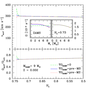
Figure 1: Evolution of the stellar rotation during the first part of the MS for the three models with 9M_☉ and $Z=0.002$ with the same value of $J_{\rm tot}$, but with different rotation profiles on the ZAMS, as described in the text. Upper panel: Equatorial rotational velocity as a function of the central mass fraction of hydrogen $H_{c}$. The internal rotation profiles on the ZAMS ($H_{c}\simeq 0.744$) and at $H_{c}=0.73$ are superimposed. Lower panel: Ratio of the surface angular velocity to the critical angular velocity as a function of the central mass fraction of hydrogen. In both panels, the two stages of the rotation profiles are indicated by vertical dotted lines.

This figure shows that the model with the flat internal rotation profile ($\nabla\Omega_{\rm ZAMS}=0$) begins its MS evolution with a sharp decrease of $v_{\rm surf}$. The strong meridional currents quickly modify the artificial flat rotation profile, producing a decrease of the surface velocity and an increase of the angular velocity in the internal regions. The same occurs with the model obtained through pre-MS calculations: despite having a differential rotation on the ZAMS, the rotation profile is not in a stationary situation either, and meridional currents act to increase $\nabla\Omega$ and decrease the surface velocity as for $\nabla\Omega_{\rm ZAMS}=0$, but in a weaker fashion, since the rotation profile is closer to a quasi-equilibrium configuration. The third model we propose at the ZAMS has an internal profile that is steeper than the as for the pre-MS calculations we described before. For this ad hoc profile, the convergence to the quasi-equilibrium configuration (hereafter initial MS rotation profile) corresponds to an increase of the surface velocity and a decrease of the angular velocity in the central regions of the star. Fig. 1 shows that very shortly after the ZAMS (4% of the MS duration), the rotation profile of the three models with the same angular momentum content has already converged to the same initial MS rotation profile. After this stage, all models evolve identically in terms of surface velocity and evolutionary tracks on the HRD.

The evolutionary tracks on the HRD of the models with the three initial conditions are shown in Fig. 2 together with a zoom on the ZAMS showing that the three different tracks converge to the same. There are only small differences in the evolutionary tracks after the MS phase when crossing to the red part of the HRD after the end of central He burning. This is because the values of $J_{\rm tot}$ in the three models are not exactly the same. The small differences in $J_{\rm tot}$ ($\simeq 0.05\%$) can produce these differences on the HR tracks in these stages that are very sensitive to the rotation properties of the star.

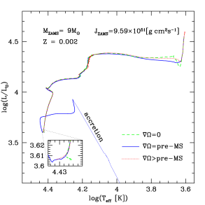
Figure 2: HR diagram of the three models with 9M_☉ and $Z=0.002$ with the same value of $J_{\rm tot}$, but with different rotation profiles on the ZAMS, as described in the text. For the model computed with the pre-MS, the part of the track corresponding to the accretion phase is indicated.

The behaviour of the equatorial rotational velocity just after the ZAMS for the different initial internal structures illustrates the reason why we need to propose an ad hoc rotation profile on the ZAMS in some cases to obtain models with a surface velocity close to the critical velocity during the whole main sequence. As shown by Haemmerlé et al. (2013) for $Z=0.014$, models with a pre-MS evolution that have M${}_{\rm ZAMS}\geq$6 M_☉ begin their MS evolution with a decrease of $\rm v_{surf}/v_{crit}$, as for $\nabla\Omega_{\rm ZAMS}=0$, but in a weaker way. For $Z=0.002$, this initial decrease of $\rm v_{surf}/v_{crit}$ occurs for the whole mass range we considered here. Where the decrease in the equatorial velocity is strong enough, a limitation in $J_{\rm tot}$ is imposed, of the same type as for $\nabla\Omega_{\rm ZAMS}=0$, so that an ad hoc steeper internal rotational profile is required at the ZAMS to be able to generate stellar models with higher values of $J_{\rm tot}$. These high initial values of angular momentum content are necessary for a rotation of the star with $\rm v_{surf}/v_{crit}$ close to one during the whole MS.

We have shown that the MS evolution of models with a steep ad hoc internal rotation profile on the ZAMS is virtually the same as the MS evolution of models with $\nabla\Omega_{\rm ZAMS}=0$. We used these ad hoc rotation profiles on the ZAMS when the rotation profile obtained from pre-MS evolution did not allow us to obtain a $\rm v_{surf}/v_{crit}$ high enough at the beginning of the MS.

The question that naturally arises is whether there is a pre-MS scenario ($\dot{M}$, $\dot{J}$), different from the one proposed here, that produces such a steep rotation profile on the ZAMS. Answering this question is beyond the scope of this article, therefore we leave this to be discussed in a forthcoming work.

Our findings are also useful because they show that models with a solid rotation profile at the ZAMS can represent the evolution of a star with the same initial angular momentum content, but any initial internal rotation profile, except at the very beginning of the MS. We should bear in mind, however, that the surface equatorial velocity when the initial MS rotation profile is reached corresponds to a lower value than the equatorial velocity for the solidly rotating model at the ZAMS.

In this sense, each model presented by Georgy et al. (2013) would adequately represent a differentially rotating star at the ZAMS with an initial rotational velocity rate $\omega$ corresponding to the rate obtained when the initial MS rotation profile is reached, which corresponds to the lowest rotational rate achieved soon after the ZAMS, when the star reaches a quasi-equilibrium state, as seen in Fig. 1.

Because we intend to understand the evolution of very rapidly rotating stars, we saught to obtain stellar evolution models with rotational rates close to critical during the whole MS. We present here rapidly rotating stellar models with a large angular momentum content and a non-flat rotational profile at the ZAMS that can soon reach the critical limit.

In the following section we compare these new stellar evolution models with large angular momentum content with the results reported by Georgy et al. (2013).

3 Results

Following what has been presented in Section 2 we can assume that each model computed asuming solid-body rotation and different rotational rate at the ZAMS (Georgy et al., 2013) evolves identically to models with the same mass, metallicity, and angular momentum content, regardless of the internal rotational profile, except for very early in the main sequence.

Because we intend to have a grid of models with initial rotation rates ranging from zero to almost critically rotating in order to be able to study the evolution of rotating stellar populations, we still need to complete the range of models for stars that rotate close to the critical limit since early in the MS. To do this, we generated models with a non-solid-body rotation profile at the ZAMS and a larger angular momentum content than those presented in Georgy et al. (2013). As explained in Section 2, for models that failed to reach these large angular momentum content through the proposed accretion scenario, an ad hoc initial rotational profile was proposed.

In this way, we produced new evolutionary tracks with initial rotational rates $\omega$ at the ZAMS higher than 0.9. In this section, we describe our new results and compare them with the grids by Georgy et al. (2013). The electronic tables for these evolutionary tracks are made available at http://obswww.unige.ch/Recherche/evol/-Database-.

Tables 1, 2, and 3 show the overall characteristics at the ZAMS and at the end of the main burning stages for models with different masses and angular momentum content at Z=0.014, Z=0.006, and Z=0.002. The format of the tables is similar to the format presented by Georgy et al. (2013), except that we provide here the initial angular momentum instead of the mean rotational velocity through the MS to make the comparison among the models straightforward. Because at the end of the He and C burning the surface velocities are low, the rotation period and the ratio between the surface and the core angular velocities are listed in these tables. As for red giant stars (Eggenberger et al., 2012), it is also possible to estimate this ratio from asteroseismic observations for more massive stars, which can set constraints on the different angular momentum transfer prescriptions in stellar evolution models. The rows that list to our new calculations with a large angular momentum content are indicated with an asterisk. The remaining rows list the older models by Georgy et al. (2013), but their initial rotational velocity and rotational rate have been corrected assuming that these quantities correspond to the initial MS rotation profile, as described in Sect. 2. The modified quantities are indicated with the symbol $\dagger$.

Figures 3 and 4 show the location in the HRD of the models with the largest angular momentum content we computed for each mass and metallicity, together with the models with the fastest rotation at the ZAMS presented previously by Georgy et al. (2013).

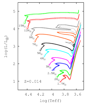
Figure 3: HRD of our models with 1.7 (red), 2 (green), 2.5 (blue), 3 (magenta), 4 (cyan), 5 (black), 7 (orange), 9 (grey), 12 (red) and 15 (green) solar masses corresponding to the largest angular momentum content (thick continuous lines) and those with the highest rotational rate at the ZAMS presented by Georgy et al. (2013) (thin dashed lines), for solar metallicity.

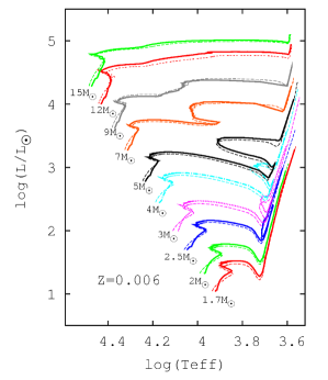
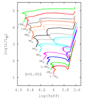
Figure 4: Same as Fig. 3, but for Z=0.006 (left) and Z=0.002 (right).

In the following subsections, we discuss the most remarkable differences and similitudes between the previously computed and the new models.

Table 1: Main parameters of A-B stars at $Z=0.014=Z_{\sun}$

				End of H-burning							End of He-burning							End of C-burning
$M_{\text{ini}}$	$\Omega/\Omega_{\text{crit, ini}}$	$v_{\text{eq}}$	$\mathcal{L}$	$\tau_{\text{H}}$	$M$	$v_{\text{eq}}$	$v_{\text{eq}}/v_{\text{crit}}$	$Y_{\text{surf}}$	$\text{N}/\text{C}$	$\text{N}/\text{O}$	$\tau_{\text{He}}$	$M$	$P_{\text{rot}}$	$\Omega_{\text{cen}}/\Omega_{\text{sur}}$	$Y_{\text{surf}}$	$\text{N}/\text{C}$	$\text{N}/\text{O}$	$\tau_{\text{C}}$	$M$	$P_{\text{rot}}$	$\Omega_{\text{cen}}/\Omega_{\text{sur}}$	$Y_{\text{surf}}$	$\text{N}/\text{C}$	$\text{N}/\text{O}$
$M_{\sun}$		km s-1	$10^{51}$ g cm2 s-1	Myr	$M_{\sun}$	km s-1		mass fract.			Myr	$M_{\sun}$	day		mass fract.			kyr	$M_{\sun}$	day		mass fract.
$15.00$	$0.00$	$0.$	${}^{\dagger}0.$	$11.015$	$14.81$	$0.$	$0.000$	$0.2660$	$0.2885$	$0.1152$	$1.315$	$13.34$	–	–	$0.3054$	$2.0811$	$0.5211$	$4.721$	$13.25$	–	–	$0.3390$	$3.0660$	$0.7360$
$15.00$	${}^{\dagger}0.43$	${}^{\dagger}188.$	${}^{\dagger}16.11$	$13.399$	$14.71$	$139.$	$0.329$	$0.2835$	$1.7907$	$0.4568$	$1.365$	$11.19$	$7.856\cdot 10^{5}$	$2.153\cdot 10^{7}$	$0.3719$	$5.5490$	$0.9928$	$2.121$	$11.07$	$1.106\cdot 10^{6}$	$2.685\cdot 10^{9}$	$0.3954$	$6.5423$	$1.1182$
$15.00$	${}^{\dagger}0.81$	${}^{\dagger}400.$	${}^{\dagger}30.90$	$14.189$	$14.66$	$287.$	$0.639$	$0.3199$	$8.1555$	$0.8963$	$1.441$	$12.63$	$5.908\cdot 10^{4}$	$2.815\cdot 10^{6}$	$0.4024$	$17.4288$	$1.3403$	$2.543$	$12.51$	$9.546\cdot 10^{4}$	$4.241\cdot 10^{8}$	$0.4208$	$20.0816$	$1.4607$
$15.00$	$0.95$	$512.$	$36.13$	$15.675$	$14.56$	$278.$	$0.629$	$0.3424$	$12.4722$	$1.0927$	$1.302$	$11.96$	$8.678\cdot 10^{4}$	$3.939\cdot 10^{6}$	$0.4338$	$25.3205$	$1.6061$	$2.302$	$11.83$	$1.487\cdot 10^{5}$	$6.112\cdot 10^{8}$	$0.4502$	$28.6042$	$1.7222$
$12.00$	$0.00$	$0.$	$0.$	$15.331$	$11.94$	$0.$	$0.000$	$0.2660$	$0.2885$	$0.1152$	$2.124$	$11.36$	–	–	$0.3007$	$1.8374$	$0.4918$	$7.858$	$11.31$	–	–	$0.3072$	$1.9788$	$0.5280$
$12.00$	${}^{\dagger}0.44$	${}^{\dagger}178.$	${}^{\dagger}10.54$	$18.540$	$11.91$	$164.$	$0.397$	$0.2755$	$1.4363$	$0.3818$	$1.892$	$10.40$	$8.402\cdot 10^{4}$	$2.809\cdot 10^{6}$	$0.3272$	$4.4674$	$0.7804$	$6.134$	$10.31$	$1.327\cdot 10^{5}$	$5.280\cdot 10^{8}$	$0.3502$	$5.3748$	$0.8895$
$12.00$	${}^{\dagger}0.82$	${}^{\dagger}385.$	${}^{\dagger}20.09$	$19.302$	$11.89$	$333.$	$0.748$	$0.3071$	$9.0862$	$0.8352$	$2.357$	$10.80$	$3.044\cdot 10^{4}$	$1.837\cdot 10^{6}$	$0.3552$	$18.2425$	$1.0840$	$0.066$	$10.73$	$4.571\cdot 10^{4}$	$5.457\cdot 10^{7}$	$0.3780$	$21.0351$	$1.1874$
$12.00$	$0.95$	$494.$	$23.33$	$21.675$	$11.83$	$323.$	$0.739$	$0.3284$	$14.1578$	$1.0083$	$2.028$	$10.53$	$4.182\cdot 10^{4}$	$2.267\cdot 10^{6}$	$0.3772$	$25.4539$	$1.2692$	$0.069$	$10.45$	$5.753\cdot 10^{4}$	$5.759\cdot 10^{7}$	$0.4010$	$29.2844$	$1.3905$
$9.00$	$0.00$	$0.$	$0.$	$26.262$	$8.99$	$0.$	$0.000$	$0.2660$	$0.2885$	$0.1152$	$3.492$	$8.80$	–	–	$0.2824$	$1.6090$	$0.4219$
$9.00$	${}^{\dagger}0.44$	${}^{\dagger}170.$	${}^{\dagger}5.98$	$31.464$	$8.99$	$170.$	$0.427$	$0.2709$	$1.0243$	$0.3023$	$3.351$	$8.76$	$1.001\cdot 10^{4}$	$3.890\cdot 10^{5}$	$0.3285$	$4.7700$	$0.7896$	$0.009$	$8.72$	$3.673\cdot 10^{4}$	$7.449\cdot 10^{7}$	$0.3290$	$4.9811$	$0.8029$
$9.00$	${}^{\dagger}0.83$	${}^{\dagger}364.$	${}^{\dagger}11.40$	$32.482$	$8.98$	$380.$	$0.888$	$0.2962$	$7.0486$	$0.7520$	$4.610$	$8.73$	$9.626\cdot 10^{3}$	$7.050\cdot 10^{5}$	$0.3296$	$15.9175$	$0.9689$
$9.00$	$0.95$	$464.$	$13.09$	$33.120$	$8.94$	$391.$	$0.903$	$0.3098$	$11.9060$	$0.8770$	$4.250$	$8.80$	$8.105\cdot 10^{3}$	$5.597\cdot 10^{5}$	$0.3465$	$25.2410$	$1.0864$
$7.00$	$0.00$	$0.$	$0.$	$41.722$	$7.00$	$0.$	$0.000$	$0.2660$	$0.2885$	$0.1152$	$6.919$	$6.92$	–	–	$0.2792$	$1.5177$	$0.3964$
$7.00$	${}^{\dagger}0.44$	${}^{\dagger}161.$	${}^{\dagger}3.59$	$51.151$	$7.00$	$160.$	$0.420$	$0.2685$	$0.7166$	$0.2341$	$6.795$	$6.89$	$4.772\cdot 10^{3}$	$2.193\cdot 10^{5}$	$0.3190$	$4.0102$	$0.7192$
$7.00$	${}^{\dagger}0.83$	${}^{\dagger}347.$	${}^{\dagger}6.87$	$52.900$	$6.99$	$362.$	$0.892$	$0.2871$	$4.3773$	$0.6282$	$8.465$	$6.89$	$2.508\cdot 10^{3}$	$2.187\cdot 10^{5}$	$0.3291$	$13.0544$	$0.9246$
$7.00$	$0.95$	$442.$	$7.79$	$54.258$	$6.96$	$360.$	$0.882$	$0.2984$	$7.3498$	$0.7410$	$8.674$	$6.87$	$3.501\cdot 10^{3}$	$2.884\cdot 10^{5}$	$0.3388$	$18.3308$	$0.9904$
$5.00$	$0.00$	$0.$	$0.$	$88.195$	$5.00$	$0.$	$0.000$	$0.2660$	$0.2885$	$0.1152$	$19.380$	$4.96$	–	–	$0.2792$	$1.4819$	$0.3864$
$5.00$	${}^{\dagger}0.44$	${}^{\dagger}150.$	${}^{\dagger}1.80$	$109.085$	$5.00$	$143.$	$0.409$	$0.2670$	$0.4995$	$0.1781$	$16.800$	$4.95$	$1.416\cdot 10^{3}$	$7.935\cdot 10^{4}$	$0.3154$	$3.3394$	$0.6627$
$5.00$	${}^{\dagger}0.83$	${}^{\dagger}325.$	${}^{\dagger}3.44$	$113.858$	$4.99$	$316.$	$0.866$	$0.2771$	$2.1374$	$0.4527$	$21.160$	$4.94$	$8.364\cdot 10^{2}$	$8.189\cdot 10^{4}$	$0.3256$	$8.1090$	$0.8382$
$5.00$	$0.95$	$419.$	$3.90$	$117.370$	$4.98$	$316.$	$0.859$	$0.2891$	$4.3180$	$0.6092$	$19.920$	$4.93$	$1.063\cdot 10^{3}$	$1.023\cdot 10^{5}$	$0.3327$	$10.9402$	$0.8951$
$4.00$	$0.00$	$0.$	$0.$	$152.088$	$4.00$	$0.$	$0.000$	$0.2660$	$0.2885$	$0.1152$	$37.750$	$3.97$	–	–	$0.2823$	$1.5023$	$0.3912$
$4.00$	${}^{\dagger}0.45$	${}^{\dagger}142.$	${}^{\dagger}1.13$	$187.477$	$4.00$	$129.$	$0.399$	$0.2666$	$0.4202$	$0.1554$	$34.852$	$3.97$	$8.134\cdot 10^{2}$	$5.097\cdot 10^{4}$	$0.3167$	$3.0686$	$0.6380$
$4.00$	${}^{\dagger}0.84$	${}^{\dagger}310.$	${}^{\dagger}2.16$	$198.351$	$3.99$	$282.$	$0.849$	$0.2743$	$1.5901$	$0.3846$	$37.370$	$3.96$	$3.954\cdot 10^{2}$	$4.232\cdot 10^{4}$	$0.3276$	$6.4637$	$0.7997$
$4.00$	$0.95$	$408.$	$2.47$	$205.350$	$3.97$	$297.$	$0.897$	$0.2859$	$3.2599$	$0.5439$	$36.264$	$3.94$	$5.206\cdot 10^{2}$	$5.311\cdot 10^{4}$	$0.3359$	$8.8096$	$0.8687$
$3.00$	$0.00$	$0.$	$0.$	$320.600$	$3.00$	$0.$	$0.000$	$0.2660$	$0.2885$	$0.1152$	$117.109$	$2.99$	–	–	$0.2868$	$1.5318$	$0.3928$
$3.00$	${}^{\dagger}0.45$	${}^{\dagger}133.$	${}^{\dagger}0.62$	$400.944$	$3.00$	$116.$	$0.395$	$0.2664$	$0.3698$	$0.1402$	$97.083$	$2.98$	$2.641\cdot 10^{2}$	$2.010\cdot 10^{4}$	$0.3213$	$2.8644$	$0.6132$
$3.00$	${}^{\dagger}0.84$	${}^{\dagger}290.$	${}^{\dagger}1.19$	$422.412$	$3.00$	$225.$	$0.748$	$0.2719$	$1.1641$	$0.3145$	$105.941$	$2.98$	$1.928\cdot 10^{2}$	$2.302\cdot 10^{4}$	$0.3314$	$5.3924$	$0.7517$
$3.00$	$0.95$	$372.$	$1.36$	$441.770$	$2.98$	$239.$	$0.797$	$0.2805$	$2.2412$	$0.4474$	$97.862$	$2.96$	$2.598\cdot 10^{2}$	$2.718\cdot 10^{4}$	$0.3406$	$7.0227$	$0.8219$
$2.50$	$0.00$	$0.$	$0.$	$537.964$	$2.50$	$0.$	$0.000$	$0.2660$	$0.2885$	$0.1152$	$236.764$	$2.49$	–	–	$0.2852$	$1.4444$	$0.3662$
$2.50$	${}^{\dagger}0.45$	${}^{\dagger}128.$	${}^{\dagger}0.43$	$665.370$	$2.50$	$109.$	$0.389$	$0.2663$	$0.3491$	$0.1338$	$185.800$	$2.49$	$2.206\cdot 10^{2}$	$1.648\cdot 10^{4}$	$0.3206$	$2.6893$	$0.5737$
$2.50$	${}^{\dagger}0.83$	${}^{\dagger}277.$	${}^{\dagger}0.82$	$704.202$	$2.50$	$228.$	$0.800$	$0.2711$	$1.0004$	$0.2816$	$194.550$	$2.48$	$1.478\cdot 10^{2}$	$1.814\cdot 10^{4}$	$0.3301$	$4.7606$	$0.6958$
$2.50$	$0.95$	$348.$	$0.94$	$745.024$	$2.49$	$200.$	$0.755$	$0.2755$	$1.5805$	$0.3629$	$195.844$	$2.47$	$1.923\cdot 10^{2}$	$1.867\cdot 10^{4}$	$0.3413$	$6.1237$	$0.7648$
$2.00$	$0.00$	$0.$	$0.$	$1008.888$	$2.00$	$0.$	$0.000$	$0.2660$	$0.2885$	$0.1152$
$2.00$	${}^{\dagger}0.46$	${}^{\dagger}125.$	${}^{\dagger}0.28$	$1267.754$	$2.00$	$105.$	$0.392$	$0.2664$	$0.3352$	$0.1294$
$2.00$	${}^{\dagger}0.83$	${}^{\dagger}258.$	${}^{\dagger}0.51$	$1340.230$	$2.00$	$210.$	$0.775$	$0.2704$	$0.7895$	$0.2373$
$2.00$	$0.96$	$337.$	$0.60$	$1427.870$	$1.99$	$189.$	$0.750$	$0.2756$	$1.3715$	$0.3270$
$1.70$	$0.00$	$0.$	$0$	$1633.971$	$1.70$	$0.$	$0.000$	$0.2660$	$0.2885$	$0.1152$
$1.70$	${}^{\dagger}0.46$	${}^{\dagger}120.$	${}^{\dagger}0.20$	$2068.535$	$1.70$	$102.$	$0.391$	$0.2664$	$0.3214$	$0.1252$
$1.70$	${}^{\dagger}0.85$	${}^{\dagger}255.$	${}^{\dagger}0.39$	$2181.676$	$1.70$	$212.$	$0.809$	$0.2711$	$0.7294$	$0.2228$
$1.70$	$0.95$	$311.$	$0.44$	$2386.735$	$1.69$	$214.$	$0.833$	$0.2805$	$1.5606$	$0.3403$

Table 2: Main parameters of A-B stars at $Z=0.006=Z_{\text{LMC}}$

				End of H-burning							End of He-burning							End of C-burning
$M_{\text{ini}}$	$\Omega/\Omega_{\text{crit, ini}}$	$v_{\text{eq}}$	$\mathcal{L}$	$\tau_{\text{H}}$	$M$	$v_{\text{eq}}$	$v_{\text{eq}}/v_{\text{crit}}$	$Y_{\text{surf}}$	$\text{N}/\text{C}$	$\text{N}/\text{O}$	$\tau_{\text{He}}$	$M$	$P_{\text{rot}}$	$\Omega_{\text{cen}}/\Omega_{\text{sur}}$	$Y_{\text{surf}}$	$\text{N}/\text{C}$	$\text{N}/\text{O}$	$\tau_{\text{C}}$	$M$	$P_{\text{rot}}$	$\Omega_{\text{cen}}/\Omega_{\text{sur}}$	$Y_{\text{surf}}$	$\text{N}/\text{C}$	$\text{N}/\text{O}$
$M_{\sun}$		km s-1	$10^{51}$ g cm2 s-1	Myr	$M_{\sun}$	km s-1		mass fract.			Myr	$M_{\sun}$	day		mass fract.			kyr	$M_{\sun}$	day		mass fract.
$15.00$	$0.00$	$0.$	$0.$	$11.097$	$14.87$	$0.$	$0.000$	$0.2559$	$0.2885$	$0.1152$	$1.338$	$14.00$	–	–	$0.2685$	$1.3634$	$0.3566$	$3.504$	$13.90$	–	–	$0.3214$	$2.7453$	$0.6739$
$15.00$	${}^{\dagger}0.43$	${}^{\dagger}195.$	${}^{\dagger}16.60$	$13.409$	$14.80$	$168.$	$0.370$	$0.2776$	$2.7679$	$0.5921$	$1.286$	$13.92$	$3.766\cdot 10^{4}$	$1.143\cdot 10^{6}$	$0.3490$	$6.5843$	$1.0305$	$2.475$	$13.80$	$6.487\cdot 10^{4}$	$1.772\cdot 10^{8}$	$0.3845$	$8.8557$	$1.2540$
$15.00$	${}^{\dagger}0.82$	${}^{\dagger}415.$	${}^{\dagger}31.94$	$16.133$	$14.68$	$308.$	$0.636$	$0.3742$	$32.4405$	$1.3712$	$1.211$	$12.33$	$1.066\cdot 10^{5}$	$4.979\cdot 10^{6}$	$0.4316$	$49.7553$	$1.6533$	$1.599$	$12.17$	$1.095\cdot 10^{5}$	$4.690\cdot 10^{8}$	$0.4707$	$58.6210$	$1.9853$
$15.00$	$0.91$	$494.$	$35.19$	$15.655$	$14.65$	$435.$	$0.897$	$0.3574$	$39.9355$	$1.2728$	$1.287$	$13.07$	$4.753\cdot 10^{4}$	$2.446\cdot 10^{6}$	$0.4093$	$57.2083$	$1.5153$	$0.083$	$12.94$	$5.451\cdot 10^{4}$	$2.696\cdot 10^{7}$	$0.4409$	$64.6910$	$1.7625$
$12.00$	$0.00$	$0.$	$0.$	$15.310$	$11.95$	$0.$	$0.000$	$0.2559$	$0.2885$	$0.1152$	$1.976$	$10.95$	–	–	$0.2667$	$1.5412$	$0.3811$	$6.465$	$10.88$	–	–	$0.2977$	$2.4608$	$0.5905$
$12.00$	${}^{\dagger}0.43$	${}^{\dagger}186.$	${}^{\dagger}10.81$	$18.395$	$11.93$	$177.$	$0.400$	$0.2699$	$2.3935$	$0.5259$	$1.910$	$11.42$	$2.350\cdot 10^{4}$	$8.443\cdot 10^{5}$	$0.3068$	$5.3803$	$0.8292$	$5.168$	$11.34$	$4.826\cdot 10^{4}$	$1.910\cdot 10^{8}$	$0.3499$	$7.7164$	$1.0572$
$12.00$	${}^{\dagger}0.82$	${}^{\dagger}399.$	${}^{\dagger}20.73$	$22.249$	$11.88$	$378.$	$0.799$	$0.3638$	$44.9194$	$1.3331$	$1.802$	$11.07$	$2.209\cdot 10^{4}$	$1.317\cdot 10^{6}$	$0.4041$	$67.7565$	$1.5184$	$0.040$	$10.98$	$3.258\cdot 10^{4}$	$2.320\cdot 10^{7}$	$0.4299$	$77.6552$	$1.6540$
$12.00$	$0.91$	$477.$	$22.97$	$22.297$	$11.84$	$432.$	$0.908$	$0.3577$	$56.0327$	$1.3291$	$1.877$	$11.29$	$1.754\cdot 10^{4}$	$1.045\cdot 10^{6}$	$0.3975$	$82.0123$	$1.5125$	$0.075$	$11.19$	$2.725\cdot 10^{4}$	$2.078\cdot 10^{7}$	$0.4221$	$91.6050$	$1.6360$
$9.00$	$0.00$	$0.$	$0.$	$25.992$	$8.99$	$0.$	$0.000$	$0.2559$	$0.2885$	$0.1152$	$3.363$	$8.65$	–	–	$0.2614$	$1.5134$	$0.3785$	$0.001$	$8.61$	–	–	$0.2736$	$1.8993$	$0.4749$
$9.00$	${}^{\dagger}0.44$	${}^{\dagger}175.$	${}^{\dagger}6.16$	$30.861$	$8.99$	$175.$	$0.410$	$0.2649$	$1.9041$	$0.4538$	$3.242$	$8.74$	$1.244\cdot 10^{4}$	$5.072\cdot 10^{5}$	$0.3103$	$6.2920$	$0.8623$	$0.047$	$8.69$	$3.279\cdot 10^{4}$	$5.744\cdot 10^{7}$	$0.3146$	$6.6121$	$0.8869$
$9.00$	${}^{\dagger}0.82$	${}^{\dagger}377.$	${}^{\dagger}11.79$	$35.516$	$8.98$	$394.$	$0.858$	$0.3296$	$33.6904$	$1.1950$	$3.504$	$8.90$	$6.221\cdot 10^{3}$	$4.743\cdot 10^{5}$	$0.3678$	$58.1684$	$1.3719$	$0.057$	$8.84$	$1.436\cdot 10^{4}$	$3.451\cdot 10^{7}$	$0.3808$	$67.9385$	$1.4335$
$9.00$	$0.92$	$453.$	$13.12$	$33.818$	$8.94$	$417.$	$0.899$	$0.3197$	$40.1316$	$1.1893$	$3.927$	$8.89$	$5.075\cdot 10^{3}$	$4.167\cdot 10^{5}$	$0.3452$	$63.9883$	$1.3233$	$0.018$	$8.84$	$1.326\cdot 10^{4}$	$5.316\cdot 10^{7}$	$0.3581$	$75.0921$	$1.3897$
$7.00$	$0.00$	$0.$	$0.$	$41.395$	$7.00$	$0.$	$0.000$	$0.2559$	$0.2885$	$0.1152$	$6.275$	$6.89$	–	–	$0.2587$	$1.3783$	$0.3438$
$7.00$	${}^{\dagger}0.44$	${}^{\dagger}166.$	${}^{\dagger}3.72$	$48.956$	$7.00$	$166.$	$0.407$	$0.2613$	$1.3475$	$0.3665$	$5.903$	$6.88$	$5.753\cdot 10^{3}$	$2.729\cdot 10^{5}$	$0.3020$	$5.2802$	$0.7972$
$7.00$	${}^{\dagger}0.82$	${}^{\dagger}358.$	${}^{\dagger}7.13$	$50.622$	$7.00$	$399.$	$0.903$	$0.2898$	$12.0638$	$0.9159$	$7.729$	$6.98$	$2.594\cdot 10^{3}$	$2.244\cdot 10^{5}$	$0.3155$	$23.9778$	$1.0888$
$7.00$	$0.92$	$432.$	$7.95$	$54.297$	$6.96$	$394.$	$0.891$	$0.3080$	$24.5605$	$1.0611$	$6.748$	$6.95$	$2.140\cdot 10^{3}$	$1.991\cdot 10^{5}$	$0.3265$	$38.3670$	$1.1710$
$5.00$	$0.00$	$0.$	$0.$	$83.169$	$5.00$	$0.$	$0.000$	$0.2559$	$0.2885$	$0.1152$	$15.908$	$4.95$	–	–	$0.2582$	$1.3024$	$0.3256$
$5.00$	${}^{\dagger}0.44$	${}^{\dagger}157.$	${}^{\dagger}1.87$	$99.280$	$5.00$	$152.$	$0.401$	$0.2588$	$0.8924$	$0.2773$	$15.334$	$4.93$	$2.292\cdot 10^{3}$	$1.291\cdot 10^{5}$	$0.2958$	$4.2339$	$0.7274$
$5.00$	${}^{\dagger}0.83$	${}^{\dagger}336.$	${}^{\dagger}3.58$	$101.879$	$5.00$	$358.$	$0.888$	$0.2728$	$4.6592$	$0.6626$	$18.136$	$4.95$	$8.985\cdot 10^{2}$	$1.009\cdot 10^{5}$	$0.3070$	$14.3721$	$0.9593$
$5.00$	$0.92$	$402.$	$3.98$	$108.060$	$4.98$	$374.$	$0.928$	$0.2908$	$10.5970$	$0.8371$	$18.044$	$4.92$	$1.426\cdot 10^{3}$	$1.527\cdot 10^{5}$	$0.3203$	$21.9276$	$1.0251$
$4.00$	$0.00$	$0.$	$0.$	$137.775$	$4.00$	$0.$	$0.000$	$0.2559$	$0.2885$	$0.1152$	$33.275$	$3.96$	–	–	$0.2623$	$1.4460$	$0.3596$
$4.00$	${}^{\dagger}0.44$	${}^{\dagger}148.$	${}^{\dagger}1.18$	$165.639$	$4.00$	$141.$	$0.396$	$0.2576$	$0.6796$	$0.2261$	$28.500$	$3.95$	$9.016\cdot 10^{2}$	$5.691\cdot 10^{4}$	$0.2970$	$3.8659$	$0.6970$
$4.00$	${}^{\dagger}0.83$	${}^{\dagger}321.$	${}^{\dagger}2.26$	$170.473$	$4.00$	$302.$	$0.810$	$0.2692$	$3.3039$	$0.5652$	$35.440$	$3.96$	$4.810\cdot 10^{2}$	$5.792\cdot 10^{4}$	$0.3085$	$11.7103$	$0.9063$
$4.00$	$0.94$	$405.$	$2.58$	$183.355$	$3.98$	$350.$	$0.951$	$0.2854$	$7.1076$	$0.7363$	$32.206$	$3.93$	$6.132\cdot 10^{2}$	$7.238\cdot 10^{4}$	$0.3222$	$16.8044$	$0.9812$
$3.00$	$0.00$	$0.$	$0.$	$276.224$	$3.00$	$0.$	$0.000$	$0.2559$	$0.2885$	$0.1152$	$91.745$	$2.98$	–	–	$0.2730$	$1.6582$	$0.4072$
$3.00$	${}^{\dagger}0.44$	${}^{\dagger}140.$	${}^{\dagger}0.65$	$335.387$	$3.00$	$126.$	$0.394$	$0.2571$	$0.5369$	$0.1880$	$77.623$	$2.97$	$4.049\cdot 10^{2}$	$2.891\cdot 10^{4}$	$0.3054$	$3.6971$	$0.6851$
$3.00$	${}^{\dagger}0.83$	${}^{\dagger}302.$	${}^{\dagger}1.25$	$348.099$	$3.00$	$272.$	$0.810$	$0.2668$	$2.4237$	$0.4789$	$83.829$	$2.97$	$1.985\cdot 10^{2}$	$2.562\cdot 10^{4}$	$0.3157$	$9.5293$	$0.8633$
$3.00$	$0.96$	$394.$	$1.45$	$377.908$	$2.98$	$276.$	$0.826$	$0.2804$	$4.7871$	$0.6456$	$76.037$	$2.95$	$2.959\cdot 10^{2}$	$3.618\cdot 10^{4}$	$0.3300$	$13.3044$	$0.9758$
$2.50$	$0.00$	$0.$	$0.$	$440.910$	$2.50$	$0.$	$0.000$	$0.2559$	$0.2885$	$0.1152$	$175.074$	$2.48$	–	–	$0.2757$	$1.6266$	$0.3952$
$2.50$	${}^{\dagger}0.44$	${}^{\dagger}134.$	${}^{\dagger}0.45$	$541.514$	$2.50$	$121.$	$0.395$	$0.2569$	$0.4771$	$0.1707$	$152.438$	$2.48$	$2.381\cdot 10^{2}$	$1.854\cdot 10^{4}$	$0.3098$	$3.5255$	$0.6559$
$2.50$	${}^{\dagger}0.83$	${}^{\dagger}289.$	${}^{\dagger}0.86$	$565.360$	$2.50$	$265.$	$0.831$	$0.2663$	$2.1052$	$0.4356$	$153.547$	$2.48$	$1.332\cdot 10^{2}$	$1.914\cdot 10^{4}$	$0.3190$	$8.3689$	$0.8175$
$2.50$	$0.92$	$345.$	$0.96$	$592.724$	$2.49$	$257.$	$0.813$	$0.2741$	$3.5273$	$0.5284$	$138.211$	$2.47$	$1.446\cdot 10^{2}$	$1.971\cdot 10^{4}$	$0.3294$	$10.8426$	$0.8588$
$2.00$	$0.00$	$0.$	$0.$	$805.801$	$2.00$	$0.$	$0.000$	$0.2559$	$0.2885$	$0.1152$
$2.00$	${}^{\dagger}0.46$	${}^{\dagger}136.$	${}^{\dagger}0.29$	$1007.382$	$2.00$	$120.$	$0.412$	$0.2571$	$0.4409$	$0.1596$
$2.00$	${}^{\dagger}0.84$	${}^{\dagger}278.$	${}^{\dagger}0.56$	$1054.389$	$2.00$	$246.$	$0.817$	$0.2671$	$1.8486$	$0.3842$
$2.00$	$0.94$	$348.$	$0.63$	$1118.312$	$1.99$	$243.$	$0.813$	$0.2760$	$3.1706$	$0.4920$
$1.70$	$0.00$	$0.$	$0.$	$1284.504$	$1.70$	$0.$	$0.000$	$0.2559$	$0.2885$	$0.1152$
$1.70$	${}^{\dagger}0.46$	${}^{\dagger}131.$	${}^{\dagger}0.21$	$1616.978$	$1.70$	$117.$	$0.413$	$0.2573$	$0.4062$	$0.1494$
$1.70$	${}^{\dagger}0.84$	${}^{\dagger}264.$	${}^{\dagger}0.41$	$1695.775$	$1.70$	$238.$	$0.812$	$0.2687$	$1.5883$	$0.3451$
$1.70$	$0.92$	$313.$	$0.46$	$1882.756$	$1.69$	$228.$	$0.792$	$0.2822$	$3.4912$	$0.4830$

Table 3: Main parameters of A-B stars at $Z=0.002=Z_{\text{SMC}}$

				End of H-burning							End of He-burning							End of C-burning
$M_{\text{ini}}$	$\Omega/\Omega_{\text{crit, ini}}$	$v_{\text{eq}}$	$\mathcal{L}$	$\tau_{\text{H}}$	$M$	$v_{\text{eq}}$	$v_{\text{eq}}/v_{\text{crit}}$	$Y_{\text{surf}}$	$\text{N}/\text{C}$	$\text{N}/\text{O}$	$\tau_{\text{He}}$	$M$	$P_{\text{rot}}$	$\Omega_{\text{cen}}/\Omega_{\text{sur}}$	$Y_{\text{surf}}$	$\text{N}/\text{C}$	$\text{N}/\text{O}$	$\tau_{\text{C}}$	$M$	$P_{\text{rot}}$	$\Omega_{\text{cen}}/\Omega_{\text{sur}}$	$Y_{\text{surf}}$	$\text{N}/\text{C}$	$\text{N}/\text{O}$
$M_{\sun}$		km s-1	$10^{51}$ g cm2 s-1	Myr	$M_{\sun}$	km s-1		mass fract.			Myr	$M_{\sun}$	day		mass fract.			kyr	$M_{\sun}$	day		mass fract.
$15.00$	$0.00$	$0.$	$0.$	$10.996$	$14.92$	$0.$	$0.000$	$0.2509$	$0.2885$	$0.1152$	$1.363$	$14.69$	–	–	$0.2538$	$1.0804$	$0.2851$	$2.143$	$14.60$	–	–	$0.3078$	$2.6821$	$0.6375$
$15.00$	${}^{\dagger}0.43$	${}^{\dagger}207.$	${}^{\dagger}17.06$	$13.174$	$14.88$	$191.$	$0.391$	$0.2757$	$4.5795$	$0.7518$	$1.323$	$14.48$	$2.390\cdot 10^{4}$	$7.992\cdot 10^{5}$	$0.3104$	$8.3919$	$1.0121$	$2.398$	$14.35$	$3.577\cdot 10^{4}$	$1.037\cdot 10^{8}$	$0.3762$	$13.5690$	$1.5163$
$15.00$	${}^{\dagger}0.82$	$447.$	${}^{\dagger}32.82$	$16.820$	$14.77$	$363.$	$0.699$	$0.4126$	$105.3703$	$1.8105$	$1.118$	$14.24$	$2.044\cdot 10^{4}$	$1.026\cdot 10^{6}$	$0.4436$	$128.1636$	$1.9873$	$1.136$	$14.05$	$2.966\cdot 10^{4}$	$1.244\cdot 10^{8}$	$0.4685$	$133.5483$	$2.1527$
$15.00$	$0.92$	$538.$	$37.15$	$16.794$	$14.71$	$410.$	$0.799$	$0.3961$	$129.2907$	$1.7362$	$1.143$	$13.92$	$2.723\cdot 10^{4}$	$1.337\cdot 10^{6}$	$0.4215$	$147.1358$	$1.8705$	$0.048$	$13.75$	$3.255\cdot 10^{4}$	$1.351\cdot 10^{7}$	$0.4612$	$141.9440$	$2.2448$
$12.00$	$0.00$	$0.$	$0.$	$15.100$	$11.97$	$0.$	$0.000$	$0.2509$	$0.2885$	$0.1152$	$1.852$	$11.91$	–	–	$0.2509$	$0.9303$	$0.2531$	$6.643$	$11.83$	–	–	$0.2900$	$2.4466$	$0.5674$
$12.00$	${}^{\dagger}0.43$	${}^{\dagger}198.$	${}^{\dagger}11.10$	$18.006$	$11.95$	$188.$	$0.395$	$0.2706$	$4.4735$	$0.7233$	$1.841$	$11.89$	$5.165\cdot 10^{3}$	$1.925\cdot 10^{5}$	$0.2733$	$4.8518$	$0.7520$	$6.206$	$11.80$	$2.328\cdot 10^{4}$	$1.093\cdot 10^{8}$	$0.3488$	$12.9178$	$1.2772$
$12.00$	${}^{\dagger}0.82$	${}^{\dagger}423.$	${}^{\dagger}21.37$	$22.266$	$11.91$	$426.$	$0.837$	$0.3957$	$132.0904$	$1.7541$	$1.645$	$11.81$	$1.157\cdot 10^{3}$	$7.235\cdot 10^{4}$	$0.4008$	$136.4635$	$1.7816$	$0.068$	$11.71$	$1.564\cdot 10^{4}$	$1.081\cdot 10^{7}$	$0.4392$	$164.1779$	$2.0035$
$12.00$	$0.93$	$523.$	$24.46$	$22.763$	$11.87$	$443.$	$0.888$	$0.3690$	$156.8571$	$1.6748$	$1.759$	$11.78$	$2.682\cdot 10^{3}$	$1.611\cdot 10^{5}$	$0.3735$	$161.4954$	$1.6988$	$0.072$	$11.68$	$1.491\cdot 10^{4}$	$1.117\cdot 10^{7}$	$0.4114$	$180.3932$	$1.9223$
$9.00$	$0.00$	$0.$	$0.$	$25.471$	$8.99$	$0.$	$0.000$	$0.2509$	$0.2885$	$0.1152$	$2.999$	$8.89$	–	–	$0.2510$	$1.2200$	$0.2935$	$0.047$	$8.85$	–	–	$0.2623$	$2.0719$	$0.4711$
$9.00$	${}^{\dagger}0.43$	${}^{\dagger}185.$	${}^{\dagger}6.35$	$30.090$	$8.99$	$180.$	$0.392$	$0.2659$	$3.9935$	$0.6728$	$3.170$	$8.97$	$2.075\cdot 10^{3}$	$8.907\cdot 10^{4}$	$0.2666$	$4.1190$	$0.6828$	$0.061$	$8.92$	$1.941\cdot 10^{4}$	$2.626\cdot 10^{7}$	$0.3065$	$10.6774$	$1.0264$
$9.00$	${}^{\dagger}0.82$	${}^{\dagger}400.$	${}^{\dagger}12.22$	$37.256$	$8.98$	$430.$	$0.878$	$0.3804$	$146.9191$	$1.7473$	$2.821$	$8.95$	$1.761\cdot 10^{2}$	$1.356\cdot 10^{4}$	$0.3838$	$150.6317$	$1.7659$	$0.076$	$8.89$	$1.064\cdot 10^{4}$	$2.167\cdot 10^{7}$	$0.4219$	$187.4874$	$1.9825$
$9.00$	$0.93$	$490.$	$13.91$	$37.818$	$8.95$	$434.$	$0.882$	$0.3777$	$190.4415$	$1.7518$	$2.969$	$8.93$	$1.132\cdot 10^{2}$	$9.112\cdot 10^{3}$	$0.3800$	$192.4962$	$1.7642$	$0.066$	$8.87$	$1.009\cdot 10^{4}$	$2.379\cdot 10^{7}$	$0.4113$	$213.4628$	$1.9412$
$7.00$	$0.00$	$0.$	$0.$	$39.945$	$7.00$	$0.$	$0.000$	$0.2509$	$0.2885$	$0.1152$	$5.570$	$6.94$	–	–	$0.2511$	$1.0737$	$0.2745$
$7.00$	${}^{\dagger}0.43$	${}^{\dagger}177.$	${}^{\dagger}3.86$	$46.821$	$7.00$	$171.$	$0.388$	$0.2615$	$3.0065$	$0.5893$	$5.565$	$6.94$	$3.677\cdot 10^{2}$	$1.780\cdot 10^{4}$	$0.2834$	$6.4559$	$0.8439$
$7.00$	${}^{\dagger}0.82$	${}^{\dagger}379.$	${}^{\dagger}7.42$	$56.509$	$7.00$	$413.$	$0.879$	$0.3450$	$93.7738$	$1.5255$	$5.101$	$6.99$	$1.665\cdot 10^{2}$	$1.608\cdot 10^{4}$	$0.3485$	$98.0867$	$1.5439$
$7.00$	$0.93$	$461.$	$8.20$	$63.425$	$6.97$	$428.$	$0.886$	$0.4209$	$227.4597$	$2.0013$	$4.153$	$6.95$	$7.462\cdot 10^{1}$	$7.133\cdot 10^{3}$	$0.4235$	$228.7656$	$2.7656$
$5.00$	$0.00$	$0.$	$0.$	$77.356$	$5.00$	$0.$	$0.000$	$0.2509$	$0.2885$	$0.1152$	$13.652$	$4.96$	–	–	$0.2513$	$1.0048$	$0.2649$
$5.00$	${}^{\dagger}0.43$	${}^{\dagger}167.$	${}^{\dagger}1.97$	$91.541$	$5.00$	$159.$	$0.384$	$0.2576$	$1.9886$	$0.4722$	$12.905$	$4.95$	$1.789\cdot 10^{3}$	$1.034\cdot 10^{5}$	$0.2793$	$5.0756$	$0.7719$
$5.00$	${}^{\dagger}0.82$	${}^{\dagger}355.$	${}^{\dagger}3.78$	$95.799$	$5.00$	$378.$	$0.853$	$0.2899$	$24.3400$	$1.1364$	$14.362$	$5.00$	$2.397\cdot 10^{2}$	$2.973\cdot 10^{4}$	$0.2925$	$26.5232$	$1.1567$
$5.00$	$0.92$	$435.$	$4.24$	$121.500$	$5.00$	$386.$	$0.858$	$0.3933$	$180.5181$	$1.7117$	$9.306$	$4.99$	$4.268\cdot 10^{2}$	$5.146\cdot 10^{4}$	$0.3986$	$187.5579$	$1.7411$
$4.00$	$0.00$	$0.$	$0.$	$124.375$	$4.00$	$0.$	$0.000$	$0.2509$	$0.2885$	$0.1152$	$26.143$	$3.97$	–	–	$0.2519$	$1.1545$	$0.2856$
$4.00$	${}^{\dagger}0.435$	${}^{\dagger}158.$	${}^{\dagger}1.25$	$148.207$	$4.00$	$150.$	$0.383$	$0.2557$	$1.5026$	$0.3932$	$22.925$	$3.96$	$1.046\cdot 10^{3}$	$6.835\cdot 10^{4}$	$0.2793$	$4.5882$	$0.7309$
$4.00$	${}^{\dagger}0.82$	${}^{\dagger}340.$	${}^{\dagger}2.40$	$152.800$	$4.00$	$376.$	$0.895$	$0.2812$	$14.8199$	$0.9692$	$27.807$	$3.96$	$5.956\cdot 10^{2}$	$7.748\cdot 10^{4}$	$0.2926$	$21.8880$	$1.0603$
$4.00$	$0.93$	$424.$	$2.69$	$172.360$	$3.99$	$350.$	$0.825$	$0.3196$	$56.9703$	$1.2015$	$24.897$	$3.94$	$9.272\cdot 10^{2}$	$1.068\cdot 10^{5}$	$0.3394$	$85.3472$	$1.2996$
$3.00$	$0.00$	$0.$	$0.$	$240.308$	$3.00$	$0.$	$0.000$	$0.2509$	$0.2885$	$0.1152$	$63.990$	$2.97$	–	–	$0.2549$	$1.4165$	$0.3226$
$3.00$	${}^{\dagger}0.44$	${}^{\dagger}150.$	${}^{\dagger}0.70$	$288.299$	$3.00$	$139.$	$0.386$	$0.2546$	$1.1508$	$0.3291$	$54.555$	$2.96$	$5.277\cdot 10^{2}$	$3.858\cdot 10^{4}$	$0.2867$	$4.9278$	$0.7500$
$3.00$	${}^{\dagger}0.82$	${}^{\dagger}318.$	${}^{\dagger}1.34$	$296.847$	$3.00$	$313.$	$0.813$	$0.2715$	$7.6469$	$0.7734$	$65.639$	$2.96$	$2.990\cdot 10^{2}$	$4.375\cdot 10^{4}$	$0.3018$	$21.9796$	$1.0155$
$3.00$	$0.93$	$394.$	$1.48$	$304.160$	$2.99$	$310.$	$0.789$	$0.2890$	$19.4074$	$0.9018$	$68.181$	$2.94$	$4.295\cdot 10^{2}$	$5.983\cdot 10^{4}$	$0.3106$	$36.2952$	$1.0292$
$2.50$	$0.00$	$0.$	$0.$	$374.191$	$2.50$	$0.$	$0.000$	$0.2509$	$0.2885$	$0.1152$	$114.955$	$2.48$	–	–	$0.2648$	$1.7337$	$0.3915$
$2.50$	${}^{\dagger}0.43$	${}^{\dagger}147.$	${}^{\dagger}0.49$	$453.569$	$2.50$	$133.$	$0.389$	$0.2542$	$0.9369$	$0.2794$	$97.722$	$2.47$	$3.093\cdot 10^{2}$	$2.553\cdot 10^{4}$	$0.2962$	$4.9999$	$0.7310$
$2.50$	${}^{\dagger}0.82$	${}^{\dagger}306.$	${}^{\dagger}0.93$	$468.888$	$2.50$	$311.$	$0.841$	$0.2695$	$5.7329$	$0.6636$	$112.967$	$2.47$	$1.663\cdot 10^{2}$	$2.674\cdot 10^{4}$	$0.3095$	$22.3530$	$0.9596$
$2.50$	$0.93$	$389.$	$1.10$	$489.630$	$2.49$	$312.$	$0.839$	$0.2837$	$12.8815$	$0.8177$	$117.680$	$2.45$	$2.375\cdot 10^{2}$	$3.423\cdot 10^{4}$	$0.3210$	$36.8810$	$1.0411$
$2.00$	$0.00$	$0.$	$0.$	$667.029$	$2.00$	$0.$	$0.000$	$0.2509$	$0.2885$	$0.1152$
$2.00$	${}^{\dagger}0.44$	${}^{\dagger}138.$	${}^{\dagger}0.32$	$825.594$	$2.00$	$134.$	$0.410$	$0.2547$	$0.8046$	$0.2451$	$194.067$	$1.97$	$2.192\cdot 10^{2}$	$2.047\cdot 10^{4}$	$0.3032$	$4.7208$	$0.6659$
$2.00$	${}^{\dagger}0.82$	${}^{\dagger}290.$	${}^{\dagger}0.61$	$871.563$	$2.00$	$298.$	$0.842$	$0.2753$	$5.6638$	$0.6399$
$2.00$	$0.94$	$375.$	$0.71$	$941.300$	$1.99$	$296.$	$0.834$	$0.2904$	$12.5988$	$0.8781$
$1.70$	$0.00$	$0.$	$0.$	$1053.592$	$1.70$	$0.$	$0.000$	$0.2509$	$0.2885$	$0.1152$
$1.70$	${}^{\dagger}0.44$	${}^{\dagger}132.$	${}^{\dagger}0.23$	$1313.265$	$1.70$	$134.$	$0.421$	$0.2552$	$0.6981$	$0.2181$
$1.70$	${}^{\dagger}0.81$	${}^{\dagger}265.$	${}^{\dagger}0.45$	$1701.731$	$1.70$	$272.$	$0.798$	$0.3111$	$12.7300$	$0.9124$
$1.70$	$0.94$	$352.$	$0.52$	$1609.072$	$1.69$	$288.$	$0.850$	$0.3061$	$15.9100$	$0.8343$

Table 4: Data for the models that reach the critical velocity during the MS.

$Z$	$M_{\text{ini}}$	$\Omega/\Omega_{\text{crit, ini}}$	$\tau_{\text{crit. rot.}}$	$\tau_{\text{crit. rot.}}/\tau_{\text{MS}}$	$H_{\text{cen}}$	$\Delta M_{\text{tot}}$	$\Delta M_{\text{rad}}$	$\Delta M_{\text{mech}}$	$\dot{M}_{\text{mech, mean}}$
	$M_{\sun}$		yr			$M_{\sun}$	$M_{\sun}$	$M_{\sun}$	$M_{\sun}\cdot\text{yr}^{-1}$
$0.014$	$1.70$	$0.95$	$1.9195\cdot 10^{9}$	$0.804$	$0.643$	$0.0979$	$0.0892$	$8.6831\cdot 10^{-3}$	$4.5236\cdot 10^{-12}$
$0.014$	$2.00$	$0.96$	$1.1401\cdot 10^{9}$	$0.809$	$0.619$	$0.0399$	$0.0310$	$8.9237\cdot 10^{-3}$	$7.8274\cdot 10^{-12}$
$0.014$	$2.50$	$0.95$	$5.3951\cdot 10^{8}$	$0.733$	$0.584$	$0.0760$	$0.0651$	$1.0933\cdot 10^{-2}$	$2.0265\cdot 10^{-11}$
$0.014$	$3.00$	$0.95$	$3.5548\cdot 10^{8}$	$0.805$	$0.622$	$0.0813$	$0.0641$	$1.7220\cdot 10^{-2}$	$4.8443\cdot 10^{-11}$
$0.014$	$4.00$	$0.95$	$1.7809\cdot 10^{8}$	$0.867$	$0.654$	$0.1238$	$0.0990$	$2.4704\cdot 10^{-2}$	$1.3872\cdot 10^{-10}$
$0.014$	$5.00$	$0.95$	$8.4680\cdot 10^{7}$	$0.721$	$0.593$	$0.1037$	$0.0756$	$2.8118\cdot 10^{-2}$	$3.3205\cdot 10^{-10}$
$0.014$	$7.00$	$0.95$	$3.7185\cdot 10^{7}$	$0.685$	$0.576$	$0.1537$	$0.1159$	$3.7842\cdot 10^{-2}$	$1.0177\cdot 10^{-9}$
$0.014$	$9.00$	$0.95$	$2.2899\cdot 10^{7}$	$0.690$	$0.578$	$0.2289$	$0.1825$	$4.6381\cdot 10^{-2}$	$2.0255\cdot 10^{-9}$
$0.014$	$12.00$	$0.95$	$1.1726\cdot 10^{7}$	$0.541$	$0.589$	$1.5632$	$1.5489$	$1.4287\cdot 10^{-2}$	$1.2184\cdot 10^{-9}$
$0.014$	$15.00$	$0.95$	$9.1153\cdot 10^{6}$	$0.582$	$0.574$	$3.1693$	$3.1637$	$5.6247\cdot 10^{-3}$	$6.1706\cdot 10^{-10}$
$0.006$	$1.70$	$0.93$	$1.3225\cdot 10^{9}$	$0.702$	$0.596$	$0.0818$	$0.0719$	$9.8766\cdot 10^{-3}$	$7.4683\cdot 10^{-12}$
$0.006$	$2.00$	$0.94$	$8.9484\cdot 10^{8}$	$0.800$	$0.636$	$0.0361$	$0.0245$	$1.1598\cdot 10^{-2}$	$1.2960\cdot 10^{-11}$
$0.006$	$2.50$	$0.92$	$3.8193\cdot 10^{8}$	$0.644$	$0.556$	$0.0385$	$0.0269$	$1.1644\cdot 10^{-2}$	$3.0486\cdot 10^{-11}$
$0.006$	$3.00$	$0.96$	$3.1073\cdot 10^{8}$	$0.822$	$0.655$	$0.0575$	$0.0399$	$1.7599\cdot 10^{-2}$	$5.6638\cdot 10^{-11}$
$0.006$	$4.00$	$0.94$	$1.2853\cdot 10^{8}$	$0.701$	$0.600$	$0.0775$	$0.0580$	$1.9500\cdot 10^{-2}$	$1.5172\cdot 10^{-10}$
$0.006$	$5.00$	$0.92$	$5.5128\cdot 10^{7}$	$0.510$	$0.500$	$0.0808$	$0.0630$	$1.7803\cdot 10^{-2}$	$3.2294\cdot 10^{-10}$
$0.006$	$7.00$	$0.92$	$2.8344\cdot 10^{7}$	$0.522$	$0.510$	$0.7640$	$0.0508$	$2.5565\cdot 10^{-2}$	$9.0195\cdot 10^{-10}$
$0.006$	$9.00$	$0.92$	$1.6014\cdot 10^{7}$	$0.474$	$0.478$	$0.1504$	$0.1235$	$2.6973\cdot 10^{-2}$	$1.6843\cdot 10^{-9}$
$0.006$	$12.00$	$0.91$	$1.1425\cdot 10^{7}$	$0.512$	$0.460$	$0.8014$	$0.7998$	$1.6202\cdot 10^{-3}$	$1.4181\cdot 10^{-10}$
$0.006$	$15.00$	$0.91$	$6.6927\cdot 10^{6}$	$0.428$	$0.395$	$2.0345$	$2.0328$	$1.7458\cdot 10^{-3}$	$2.6084\cdot 10^{-10}$
$0.002$	$1.70$	$0.94$	$1.1390\cdot 10^{9}$	$0.708$	$0.667$	$0.0668$	$0.0556$	$1.1169\cdot 10^{-2}$	$9.8063\cdot 10^{-12}$
$0.002$	$2.00$	$0.94$	$7.2368\cdot 10^{8}$	$0.769$	$0.668$	$0.0356$	$0.0256$	$1.0052\cdot 10^{-2}$	$1.3890\cdot 10^{-11}$
$0.002$	$2.50$	$0.93$	$3.4795\cdot 10^{8}$	$0.711$	$0.616$	$0.0836$	$0.0736$	$9.9490\cdot 10^{-3}$	$2.8593\cdot 10^{-11}$
$0.002$	$3.00$	$0.93$	$1.6575\cdot 10^{8}$	$0.545$	$0.540$	$0.0813$	$0.0715$	$9.8707\cdot 10^{-3}$	$5.9551\cdot 10^{-11}$
$0.002$	$4.00$	$0.93$	$9.0014\cdot 10^{7}$	$0.522$	$0.505$	$0.0876$	$0.0756$	$1.1992\cdot 10^{-2}$	$1.3322\cdot 10^{-10}$
$0.002$	$5.00$	$0.92$	$5.1098\cdot 10^{7}$	$0.421$	$0.366$	$0.0510$	$0.0412$	$9.7813\cdot 10^{-3}$	$1.9142\cdot 10^{-10}$
$0.002$	$7.00$	$0.93$	$1.9022\cdot 10^{7}$	$0.300$	$0.235$	$0.0626$	$0.0451$	$1.7543\cdot 10^{-2}$	$9.2228\cdot 10^{-10}$
$0.002$	$9.00$	$0.93$	$2.3485\cdot 10^{7}$	$0.621$	$0.562$	$0.1365$	$0.1042$	$3.2377\cdot 10^{-2}$	$1.3786\cdot 10^{-9}$
$0.002$	$12.00$	$0.93$	$1.5147\cdot 10^{7}$	$0.665$	$0.576$	$0.3303$	$0.2946$	$3.5740\cdot 10^{-2}$	$2.3595\cdot 10^{-9}$
$0.002$	$15.00$	$0.92$	$1.0951\cdot 10^{7}$	$0.652$	$0.547$	$1.2601$	$1.1999$	$6.0194\cdot 10^{-2}$	$5.4964\cdot 10^{-9}$

3.1 Stellar lifetimes, mass of the convective cores, and evolutionary tracks in the HRD

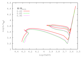
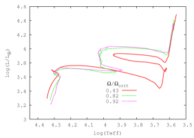
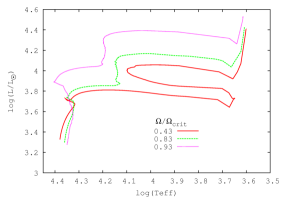
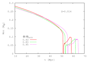
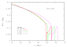
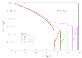
Figure 5: HRD (top) and evolution of the mass of the convective core (bottom) of 7 M_☉ models with metallicities of Z=0.014 (left), Z=0.006 (center), and Z=0.002 (right), for different rotational rates at the ZAMS.

As shown by Meynet & Maeder (2000), Ekström et al. (2008), and Georgy et al. (2013), when they are governed by the centrifugal force at the ZAMS, rotating models behave like lower mass models, with a shift of the tracks towards lower L and T_eff, compared with non-rotating models. This implies that the size of the convective core on the ZAMS decreases as a function of the initial rotational velocity. Later in the evolution, the core is fed with fresh hydrogen by the effects of rotational mixing, slowing down the decrease in the mass of the convective core (M_cc), and the newly produced helium is brought to the radiative zone, and accordingly our models evolve on bluer and more luminous tracks. Figure 5 shows the evolutionary tracks (top) and the evolution of the M_cc (bottom) of 7 M_☉ models. As already shown by Georgy et al. (2013), we find an extreme behaviour for our lower metallicity models: during the MS of the models with the highest rotational rate at the ZAMS (or in other words the models with the largest angular momentum content), the core is nourished with fresh hydrogen brought by rotational mixing in such a way that the star evolves at almost constant M_cc. Consequently, the MS lifetimes are significantly longer (see Figure 5, bottom). For the 7 M_☉ model with the largest angular momentum we computed at Z=0.002, the mixing of chemical species during the critical rotation phase is extremely efficient in the whole star. This increases the mean molecular weight $\mu$ in the external layers of the star, which has a well-known effect on its effective temperature and luminosity, shifting it bluewards in the HRD. This bluewards evolution, is typically known as chemically homogeneous evolution (Maeder, 1987; Yoon & Langer, 2005) (Figure 5, top right).

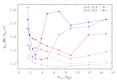
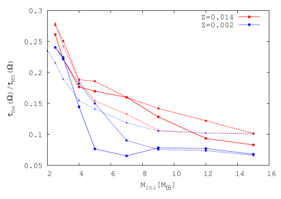
Figure 6: Extension of the MS duration (top) and helium-burning phase (bottom) with respect to the non-rotating case for Z=0.014 (red) and Z=0.002 (blue), for clarity we did not plot the results for Z=0.006, which behave much like Z=0.014. Three rotational velocity rates are shown: $\sim$0.43% (dotted line), $\sim$0.83% (dashed line) and higher than 90% of critical (continuous line).

The dependence of the MS duration of our new models with mass follows the same trend as was found for lower rotational rates: because rotational mixing increases the MS lifetimes, at Z=0.014 the increase amounts to about 15%-25% compared with the non-rotating model for stars rotating below 0.5 of the critical limit, whereas for the most rapid rotators we computed, the variation in the duration of the main sequence can be as high as 45%, as seen in Figure 6 (top). For lower metallicities, at Z=0.002 the effects of rotation in the duration of the MS are very strong, with an increase of more than 25% for all masses at high rotational rates. Our Z=0.006 models behave much like the solar metallicity case. For the smallest and largest masses we computed, this increase of the MS lifetime is higher than 55%. The duration of the helium-burning phase relative to the MS phase decreases with mass and is shorter for Z=0.002. At this metallicity, for masses below 5 M_☉ the star burns helium for a significant time, and undergoes a blue loop, which starts when the star is a red supergiant (RSG). For higher masses, as remarked by Georgy et al. (2013), rapid rotation leads the star to evolve directly to the top of the loop, without the first RSG phase. In this case, most of the core He burning occurs in the blue part of the HRD.

3.2 Surface abundances

The changes of surface abundances of CNO reflect the actions of the dominating burning cycle and the mixing mechanisms that occurr in the star. Przybilla et al. (2010) showed that a simple analytical derivation from the CNO cycle for intermediate mass stars, when the effects of mixing remain modest, leads to a linear relation between the relative enrichments N/C vs. N/O, with a slope $\sim$ 4 (see also Maeder et al., 2014). We show in Figs. 7, 8, and 9 the N/C vs. N/O diagram for Z=0.014, Z=0.006 and Z=0.002, respectively, for different initial rotational rates and different stellar masses, at the end of the MS and at the end of the helium-burning phase. The slowly rotating models ($\Omega/\Omega_{\rm crit}<0.5$) follow the linear trend described in Przybilla et al. (2010). Our new rapidly rotating models (magenta) show strong changes in the surface abundances already at the end of the MS. This is particularly remarkable for Z=0.002, as was already discussed by Georgy et al. (2013).

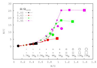
Figure 7: Surface nitrogen to carbon mass ratio versus the nitrogen to oxygen ratio at the end of hydrogen burning (circles) and end of helium burning (squares), for different stellar masses at Z=0.014. As shown at the bottom, different symbol sizes indicate different stellar masses, from 1.7 M_☉ up to 15 M_☉.

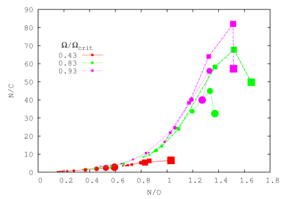
Figure 8: Same as Figure 7, but with Z=0.006. The non-rotating case is not shown in this plot.

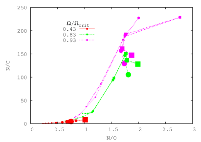
Figure 9: Same as Figure 7, but with Z=0.002. The non-rotating case is not shown in this plot.

For the helium surface abundances, Przybilla et al. (2010) showed that MS B-type stars show a roughly constant value ($\sim$ 0.28), while higher enrichments are obtained for more evolved objects, between 0.3 and 0.4. Figures 10 and 11 show the helium enrichment versus the ratio N/O at the end of the MS and at the end of the helium burning for Z=0.014 and Z=0.002. At Z=0.014, our slowly rotating models have a roughly constant helium content at the end of the MS ($\sim$ 0.27-0.3) that is close to the observed values mentioned above, in particular for models with masses smaller than 12 M_☉. For models with the largest masses and rotational rates at the ZAMS the enrichment is somewhat higher, reaching values expected for post-MS objects.

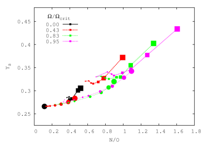
Figure 10: Helium surface abundance (Ys) versus the ratio N/O for stars at the end of the MS (circles) and at the end of the helium burning (squares) for models at Z=0.014 with different masses, represented by different point sizes as in Fig. 7, and different rotational rates at the ZAMS by different colours.

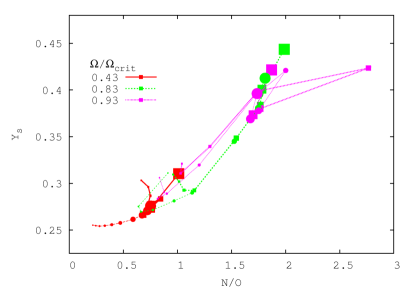
Figure 11: Same as Figure 10, but for Z=0.002.

The surface nitrogen enrichments for our rotating models are shown in Figure 12. For the metallicities presented here, the enhancements obtained for the most massive and most rapidly rotating models would be more likely to be detected, in particular towards the end of the MS.

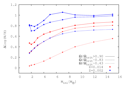
Figure 12: N/H abundance at the end of the main sequence for Z=0.002 (blue) and Z=0.014 (red) and three rotational velocities: $\sim$0.43% (dotted line), $\sim$0.83% (dashed line), and larger than 90% of critical (continuous line).

Even though the chemical enrichments might be detectable in stars, there are very few massive stars that have been critical rotators throughout their whole MS to reach the highest values presented in this work. If a MS B-type star rotating close to its critical limit were observed, it would only show a high enrichment either if it were very close to their TAMS or if it had been rotating almost critically during most of its lifetime. Early B-type stars with large V $sin$i that are close to their TAMS are good candidates in which to search for surface enrichments.

3.3 Evolution of surface velocities and mechanical mass loss

All our new rapidly rotating models with Z=0.002, Z=0.006, and Z=0.014 with masses smaller than 15 M_☉ reach the critical limit soon after the ZAMS, and therefore they lose mass mechanically during a longer time of the MS than the models presented by Georgy et al. (2013), and the duration of the MS phase is prolonged. The most massive stars, reach the critical limit, but soon stellar winds become efficient in removing the excess of angular momentum at the stallar surface, preventing the star from reaching the critical limit. Table 4 shows the duration of the critical rotation phase, the central hydrogen abundance when critical rotation is attained, the total mass lost for these models, the mass lost via stellar winds and mechanically, and also the mean mechanical mass-loss rate during the critical phase for our new computations. In all the cases, for each mass and metallicity the mean mass-loss rates throughout the critical rotation phase remain very similar to the rates we had obtained for models presented in Granada et al. (2013) with the largest angular momentum content. We exemplify in Figure 13 the evolution of the equatorial velocity through the MS phase for 7 M_☉ and 15 M_☉ models for different rotational rates at the ZAMS and for two different metallicities Z=0.002 and Z=0.014. We plot our new models that rotate significantly faster throughout the MS than our previous computations with the highest rotational rate at the ZAMS. The extension in the duration of the MS lifetime is quite remarkable as well, in particular at Z=0.002: at this metallicity, the duration of the MS for the models with a large angular momentum content is even longer than at Z=0.014. For the model with 7M_☉, the time spent on the MS is close to 20% longer.

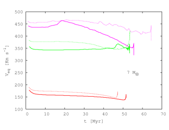
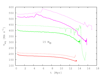
Figure 13: Evolution of the equatorial velocity through the MS phase for 7 M_☉ and 15 M_☉ models. Continuous lines correspond to Z=0.014, whereas dashed lines correspond to Z=0.002. Different colours indicate different values of $\Omega/\Omega_{\rm crit}$ at the ZAMS: red corresponds to $0.43$, green to $0.83$, and magenta to our new models with a large angular momentum content.

3.4 Metallicity dependency of the surface velocity at the ZAMS

Figure 14: Equatorial velocity at the ZAMS versus the angular momentum content for different masses and metallicities, red squares correspond to Z=0.014, green triangles to Z=0.006, and blue circles correspond to Z=0.002.

Figure 14 shows the initial angular momentum content versus the rotational velocity at the ZAMS for the models presented in Tables 1 and 3. We see that the equatorial rotational velocity at the ZAMS is almost metallicity independent, for the same mass and the same angular momentum content. This is a counterintuitive finding. Because of the differences in opacity, a star at the ZAMS at Z=0.002 is more compact than a star of identical mass at Z=0.014. We would expect the more compact star to have a smaller momentum of inertia, and therefore, a faster rotation for a given angular momentum content. We explain below that this is not the case, according to our models.

The total angular momentum of the star is given by

$$J=\int_{\star}\rho\,j\,d^{3}x={8\over 3}\pi\int_{0}^{R}\rho\,r^{4}\,\Omega\,dr,$$ (2)

where $j$ and $\rho$ are the local specific angular momentum and density. Calling $s=r/R$ and $\bar{\rho}=M/({4\over 3}\pi R^{3})$, it follows

$$J=2MR\,{\rm v_{surf}}\int_{0}^{1}{\rho\over\bar{\rho}}\,{\Omega\over\Omega_{\rm surf}}\,s^{4}\,ds.$$ (3)

Eq. (3) shows that for two stars with the same $M$ and $J$, their radii and surface velocities are related by

$$R_{1}\times{\rm v_{surf\,1}}=R_{2}\times\rm v_{surf\,2},$$ (4)

if the relative distribution of the mass (i.e. $\rho/\bar{\rho}$ as a function of $s$) and of the internal angular velocity profile ($\Omega/\Omega_{\rm surf}$ as a function of $s$) inside the star are the same.

Observations show that stars in the SMC rotate on average $\sim 20-30\%$ faster (in $\rm v_{surf}$), than stars in the Milky Way for the mass range considered here (e.g. Martayan et al., 2007). These observations, together with the compactness of stars at lower metallicities, is normally interpreted as satisfying Eq. (4), giving a ratio

$${{\rm v_{surf\,02}}\over{\rm v_{surf\,14}}}={R_{14}\over R_{02}}\simeq 1.2-1.3,$$ (5)

where $\rm v_{surf}$ indicates the equatorial surface velocity and the subscript $02$ and $14$ indicate SMC and solar metallicities, respectively, in agreement with the observations. As explained above, this relation implicitely assumes that the relative distribution of the mass and of the angular velocity inside stars of different metallicities are the same.

Since we obtain from our models at the ZAMS that ${\rm v_{surf\,02}}\simeq{\rm v_{surf\,14}}$ and $R_{14}\neq R_{02}$, we expect that the relative distribution of the mass and/or of the angular velocity must differ between both metallicities. We briefly show here that what differs between models of different metallicities is the mass distribution.

We compare two models with $Z=0.014$ and $Z=0.002$, with the same mass and angular momentum content at the ZAMS, $M_{\rm ZAMS}=9\,M_{\sun}$ and $J_{\rm ZAMS}=6.81\times 10^{51}\rm\,g\,cm^{2}\,s^{-1}$. In these two cases the internal rotation profile is differential. For these given quantities, the stellar radii and equatorial velocities are for the larger metallicity, $R_{14}=3.71\,R_{\sun}$ and ${\rm v_{surf\,14}}=198\rm\ km\,s^{-1}=35\%\rm\,v_{crit\,14}$, while for Z=0.002 they are $R_{02}=3.02\,R_{\sun}$ and ${\rm v_{surf\,02}}=203\rm\ km\,s^{-1}=33\%\rm\,v_{crit\,02}.$ The ratios presented above are ${R_{14}\over R_{02}}=1.23$ and ${\rm v_{surf\,02}\over v_{surf\,14}}=1.03$, and therefore ${R_{14}\over R_{02}}\neq{\rm v_{surf\,02}\over v_{surf\,14}}$.

We compare this result with the case of solid-body rotation, $\Omega^{\rm sol}=\Omega_{\rm surf}^{\rm sol}$, with identical characteristics as above ($M$, $J$, density profiles and radii). In this case Eq. (3) reads

$$J=2MR\,{\rm v_{surf}^{\rm sol}}\int_{0}^{1}{\rho\over\bar{\rho}}\,s^{4}\,ds.$$ (6)

Replacing this with the known quantities and integrating Eq. (6) for the two metallicities, we obtain:

$${R_{14}\,{\rm v_{surf\,14}^{\rm sol}}\over R_{02}\,{\rm v_{surf\,02}^{\rm sol}}}={\int_{0}^{1}{\rho_{02}\over\bar{\rho}_{02}}\,s^{4}\,ds\over\int_{0}^{1}{\rho_{14}\over\bar{\rho}_{14}}\,s^{4}\,ds}={0.040\over 0.034}=1.18.$$ (7)

Because we know that ${R_{14}\over R_{02}}=1.23$, the velocity ratio is ${\rm v_{surf\,02}^{\rm sol}\over v_{surf\,14}^{\rm sol}}=1.03$, the same as we found for a differential rotation profile.

This result shows that the difference between ${R_{14}\over R_{02}}$ and ${\rm v_{surf\,02}\over v_{surf\,14}}$ is fully explained by a difference in the distribution of mass inside the star.

A complete study of this effect and its causes for a wider range in mass and metallicity is postponed to a forthcoming paper (Haemmerlé et al. in prep.). We recall again that in the context of rotating stellar populations environments with lower metallicity than solar, such as that of the SMC, are claimed to give rise to stars that rotate faster (e.g. Keller, 2004; Martayan et al., 2007). If higher rotational velocities were actually more likely to occur at the ZAMS at Z=0.002 than at Z=0.014, and our single evolutionary models were adequate to describe the characteristics of rapidly rotating stars, this would mean that low-metallicity environments form stars with a larger angular momentum content.

3.5 Impact on the expected number of rapidly rotating B-type stars with time.

We have shown throughout this work that rotating models computed assuming solid rotation at the ZAMS adequately represent models with identical metallicity, mass, and angular momentum content, but with a differentially rotating internal profile, except for very early in the MS. Our pre-MS computations showed that the internal rotational profile has reached a quasi-stationary profile already at the ZAMS. This is the same internal rotational profile obtained after the sharp decrease in the surface velocity of our models with a flat profile at the ZAMS. Therefore, we propose to use the grids presented by Georgy et al. (2013) (assuming that the rotational rate at the ZAMS is the rate when the quasi-equilibrium has been reached) together with our new models of very rapidly rotating stars throughout the MS, to study how rotating stellar populations evolve in time, as we have already done in Granada et al. (2013), by using the new Geneva population synthesis code (SYCLIST, for synthetic clusters, isochrones, and stellar tracks) presented by Georgy et al. (2014).

We studied how the fraction of stars with surface velocities above a given limit varies in clusters of various ages. We briefly recall that the populations are computed in the mass domain of 1.7 - 15 M_☉ with initial rotational rates between 0 and 1. We discretized the mass domain into 1000 mass intervals and the velocity domain into 100 intervals.

Each mass and velocity cell was assigned with the expected number of stars and then normalised according to an initial mass function (Salpeter, 1955) and to an initial rotation-rate distribution (Huang et al., 2010). We then built an evolutionary track for these initial conditions and interpolated between our computed tracks. At each timestep, we checked the spectral type of the star in each of the cells, and its current rotation rate. If the star was in the B-type domain and the rotation rate was higher than a given constant (0.70, 0.90, or 0.98), we added the number of stars in the cell to the total number of stars of a given spectral type that rotates more rapidly than the given constant. The population was normalised with respect to the total number of B stars at the same time.

Even though the distribution by Huang et al. (2010) was obtained for Z=0.014, we used it as well to produce a population at Z=0.002 to compare this with our previous results and study the effects of metallicity alone. An identical initial distribution of rotational rates for both metallicities corresponds to a distribution of higher rotational velocities at the ZAMS for Z=0.002. This corresponds to a larger angular momentum content for objects at lowe metallicities, which is in principle coherent with observations of rotating B-type stars.

Figures 15 and 16 show the time evolution of stars rotating faster than 0.70, 0.90, and 0.98 in terms of $\Omega/\Omega_{crit}$ (these values correspond to 0.51, 0.73, and 0.88 in terms of $v/v_{crit}$, respectively) for Z=0.002 and Z=0.014.

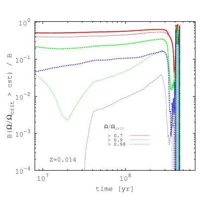
Figure 15: Time evolution of the fraction of B-type stars that rotate faster than a certain $\Omega/\Omega_{crit}$ for Z=0.014. Red continuous lines correspond to the fraction of stars rotating with $\Omega/\Omega_{crit}$¿0.7, green dashed lines to those with $\Omega/\Omega_{crit}$¿0.9, and blue dotted lines to $\Omega/\Omega_{crit}$¿0.98. Thin lines correspond to the ZAMS rotational rates for solidly rotating models shown in Granada et al. (2013), whereas the thicker lines are our new results obtained assuming that the rotational rate at the ZAMS is the rate when the quasi-equilibrium has been reached.

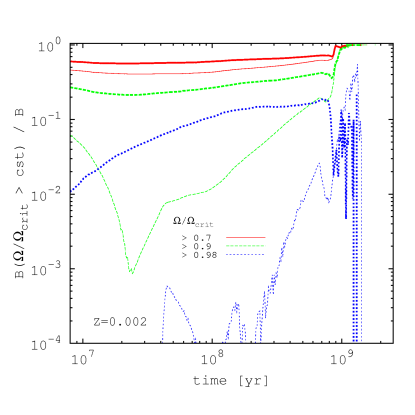
Figure 16: Idem. figure 15 but for Z=0.002.

As expected, our new results lead to higher percentages of rapidly rotating stars. The effect is moderate for the fraction of stars rotating with $\Omega/\Omega_{crit}$¿0.7, whereas the changes are strong for the group of the most rapidly rotating stars. We find now that there is always a non-zero probability of having stars rotating with $\Omega/\Omega_{crit}$¿0.98 at all ages, which can become higher than 10% of B stars towards the TAMS of late B-type stars, where the existing B stars are rapidly rotating objects.

4 Conclusions

We have shown that our grids of rotating models computed assuming solid rotation at the ZAMS (Georgy et al., 2013) adequately represent models with a different initial internal rotation profile, but identical metallicity, mass, and angular momentum content, except for very early in the MS. We propose to use these grids in the future to build synthetic populations, assuming as the initial rotational velocity the velocity obtained when the star has reached the quasi-equilibrium state described in Section 2.2.

By using differentially rotating stellar models at the ZAMS obtained from pre-MS calculations, we were able to produce stellar evolution models with larger angular momentum than those presented in our previous work for three different metallicities and masses between 1.7 and 15 M_☉. Objects that are rotating close to the critical rotational rate throughout the whole MS have a more extreme behaviour than those that reach the critical limit later in the MS. This is particularly important in low-metallicity environments, in which the stellar lifetimes, the evolutionary tracks in the HRD, and the surface enrichment are strongly modified by the effects of rapid rotation throughout the MS.

Interestingly and counterintuitively, we found that for a certain mass and angular momentum content, the equatorial velocity at the ZAMS depends very weakly on the metallicity. This is basically due to differences in the internal mass distribution. We will discuss this result thoroughly in a forthcoming paper (Haemmerlé et al., in preparation).

We count now on models with a large angular momentum content that rotate close to the critical limit throughout the whole MS. Our next step will be to use these new models together with the grids by Georgy et al. (2013) to compare synthetic rotating stellar populations with SYCLIST, obtained with the new Geneva population synthesis code (Georgy et al., 2014), with observed rotating populations.

References

• Arnett & Meakin (2011) Arnett, W. D. & Meakin, C. 2011, ApJ, 741, 33
• Behrend & Maeder (2001) Behrend, R. & Maeder, A. 2001, A&A, 373, 190
• Churchwell (1999) Churchwell, E. 1999, in NATO ASIC Proc. 540: The Origin of Stars and Planetary Systems, ed. C. J. Lada & N. D. Kylafis, 515
• Deupree et al. (2012) Deupree, R. G., Castañeda, D., Peña, F., & Short, C. I. 2012, ApJ, 753, 20
• Eggenberger et al. (2008) Eggenberger, P., Meynet, G., Maeder, A., et al. 2008, Ap&SS, 316, 43
• Eggenberger et al. (2012) Eggenberger, P., Montalbán, J., & Miglio, A. 2012, A&A, 544, L4
• Ekström et al. (2012) Ekström, S., Georgy, C., Eggenberger, P., et al. 2012, A&A, 537, A146
• Ekström et al. (2008) Ekström, S., Meynet, G., Maeder, A., & Barblan, F. 2008, A&A, 478, 467
• Espinosa Lara & Rieutord (2011) Espinosa Lara, F. & Rieutord, M. 2011, A&A, 533, A43
• Georgy et al. (2013) Georgy, C., Ekström, S., Granada, A., et al. 2013, A&A, 553, A24
• Georgy et al. (2014) Georgy, C., Granada, A., Ekström, S., et al. 2014, A&A, 566, A21
• Georgy et al. (2011) Georgy, C., Meynet, G., & Maeder, A. 2011, A&A, 527, A52
• Granada et al. (2013) Granada, A., Ekström, S., Georgy, C., et al. 2013, A&A, 553, A25
• Haemmerlé et al. (2013) Haemmerlé, L., Eggenberger, P., Meynet, G., Maeder, A., & Charbonnel, C. 2013, A&A, 557, A112
• Heger et al. (2000) Heger, A., Langer, N., & Woosley, S. E. 2000, ApJ, 528, 368
• Henning et al. (2000) Henning, T., Schreyer, K., Launhardt, R., & Burkert, A. 2000, A&A, 353, 211
• Huang et al. (2010) Huang, W., Gies, D. R., & McSwain, M. V. 2010, ApJ, 722, 605
• Keller (2004) Keller, S. C. 2004, PASA, 21, 310
• Maeder (1987) Maeder, A. 1987, A&A, 178, 159
• Maeder (2009) Maeder, A. 2009, Physics, Formation and Evolution of Rotating Stars
• Maeder et al. (2014) Maeder, A., Przybilla, N., Nieva, M.-F., et al. 2014, A&A, 565, A39
• Martayan et al. (2007) Martayan, C., Frémat, Y., Hubert, A.-M., et al. 2007, A&A, 462, 683
• Meynet et al. (2013) Meynet, G., Ekström, S., Maeder, A., et al. 2013, in Seismology for studies of stellar rotation and convection, Lecture Notes in Physics, Berlin Springer Verlag (Berlin: Springer Verlag)
• Meynet & Maeder (2000) Meynet, G. & Maeder, A. 2000, A&A, 361, 101
• Neiner et al. (2012) Neiner, C., Mathis, S., Saio, H., et al. 2012, A&A, 539, A90
• Przybilla et al. (2010) Przybilla, N., Firnstein, M., Nieva, M. F., Meynet, G., & Maeder, A. 2010, A&A, 517, A38
• Rivinius et al. (2013) Rivinius, T., Carciofi, A. C., & Martayan, C. 2013, A&A Rev., 21, 69
• Sackmann & Anand (1970) Sackmann, I.-J. & Anand, S. P. S. 1970, ApJ, 162, 105
• Salpeter (1955) Salpeter, E. E. 1955, ApJ, 121, 161
• Slettebak (1966) Slettebak, A. 1966, ApJ, 145, 126
• Yoon & Langer (2005) Yoon, S.-C. & Langer, N. 2005, A&A, 443, 643
• Zahn (1992) Zahn, J.-P. 1992, A&A, 265, 115