A Variable Polytrope Index Applied to Planet and Material Models

Abstract

We introduce a new approach to a century old assumption which enhances not only planetary interior calculations but also high pressure material physics. We show that the polytropic index is the derivative of the bulk modulus with respect to pressure. We then augment the traditional polytrope theory by including a variable polytrope index within the confines of the Lane-Emden differential equation. To investigate the possibilities of this method we create a high quality universal equation of state, transforming the traditional polytrope method to a tool with the potential for excellent predictive power. The theoretical foundation of our equation of state is the same elastic observable which we found equivalent to the polytrope index, the derivative of the bulk modulus with respect to pressure. We calculate the density-pressure of six common materials up to $10^{18}$ Pa, mass-radius relationships for the same materials, and produce plausible density-radius models for the rocky planets of our solar system. We argue that the bulk modulus and its derivatives have been under utilized in previous planet formation methods. We constrain the material surface observables for the inner core, outer core, and mantle of planet Earth in a systematic way including pressure, bulk modulus, and the polytrope index in the analysis. We believe this variable polytrope method has the necessary apparatus to be extended further to gas giants and stars. As supplemental material we provide computer code to calculate multi-layered planets.

1 Introduction

As more exoplanets are discovered (Françoise Roques, 2015), the need for a systematic method for planetary models becomes more pronounced (Zapolsky & Salpeter, 1969; Stacey & Davis, 2004; Valencia et al., 2006, 2007a; Sotin et al., 2007; Seager et al., 2007; Grasset et al., 2009; Leconte & Chabrier, 2012; Swift et al., 2012; Wagner et al., 2012; Zeng & Sasselov, 2013; Alibert, 2014). Our planet formation approach begins with the well known polytrope assumption at its foundation. A polytrope is a simple structural assumption between a material’s pressure and volume, $PV^{n}=C$, or similarly it’s pressure and density, $P=C\rho^{n}$, where the $C$ is a constant and $n$ is the polytrope index.

There have been some attempts to quantify what the polytrope index represents in the limited context of the ideal gas law (Chandrasekhar, 1939; Horedt, 2004). There have been other recent endeavors to import physical meaning to the polytrope index (de Sousa & de Araujo, 2011; Christians, 2012) but their results were limited in scope. To our knowledge, this work exhumes for the first time the physical definition of the polytrope index in the general case for all materials.

In the body of this article we will first derive the physical interpretation of the polytrope index as the pressure derivative of the bulk modulus and show its kinship to the Murnaghan equation of state (EOS) (Murnaghan, 1944). We then define a new variation of the traditional Lane-Emden equation in Sect. 2 and apply it in Sect. 3 by fitting the density-pressure profile of the Earth constructed from seismic data. Finding this technique limiting we then permit the polytrope index to vary, modify the Lane-Emden equation which incorporates it, and apply this variable index technique to experimental high pressure-density curves for six common planetary materials up to $10^{18}Pa$ in Sect. 4. We then, using the same theory, develop a systematic approach for planetary models and calculate Mercury, Venus, Earth, and Mars (Sect. 5). Analyzing our EOS relative to previous universal EOSs, we spotlight the functional form of the polytrope index. This survey is done to elucidate the important utility this observable has in the future development of more sophisticated formation models. We finally examine the power of this technique by scrutinizing the interior of the Earth in Sect. 7 where we constrain, with mixed success, elastic material observables extrapolated to the surface of our planet. We conclude reviewing the potential of this variable polytrope approach.

2 The polytrope index is a derivative of the Bulk Modulus

Starting with the definition of the bulk modulus ($B$), the inverse of the more intuitive compressibility ($K$), we manipulate:

from $$B=K^{-1}=\rho\frac{dP}{d\rho},$$

then $$K^{-1}\frac{d\rho}{dP}=\rho,$$

then $$\frac{dK}{dP}K^{-1}\frac{d\rho}{dP}=\frac{dK}{dP}\rho,$$ (1)

and by using the relationship, $\frac{dK}{dP}K^{-1}=-\frac{dK^{-1}}{dP}K=-\frac{dB}{dP}K$ we are able to progress to

$$\frac{dB}{dP}K\frac{d\rho}{dP}=-\frac{dK}{dP}\rho$$ (2)

and multiplying both sides by the awkward $\rho^{\frac{dB}{dP}-1}$ ($\frac{dB}{dP}$ is dimensionless)

$$\rho^{\frac{dB}{dP}-1}\frac{dB}{dP}K\frac{d\rho}{dP}=-\frac{dK}{dP}\rho^{\frac{dB}{dP}}$$

$$\mbox{then }\rho^{\frac{dB}{dP}-1}\frac{dB}{dP}K\frac{d\rho}{dP}+\frac{dK}{dP}\rho^{\frac{dB}{dP}} = 0.$$ (3)

Though this looks complicated we are able to notice a derivative power relationship of the form $\frac{d}{dP}(X^{n}Y)=X^{n-1}nY\frac{dX}{dP}+\frac{dY}{dP}X^{n}$ and so we have the intermediate result

$$\frac{d}{dP}(\rho^{\frac{dB}{dP}}K)=0\;\;\mathrm{or}\;\;\rho^{\frac{dB}{dP}}K=C^{\prime},$$ (4)

where $C^{\prime}$ is a constant. From the $P=0$ boundary condition we have

$$C^{\prime}=\rho_{0}^{({\frac{dB}{dP}})_{0}}K_{0}=\rho_{0}^{n}K_{0}=\rho^{\frac{dB}{dP}}K,$$ (5)

where the naught subscript represents the values of these variables at zero pressure. This derivation only requires that the exponent, the pressure derivative of the bulk modulus, remains constant because a simple derivative power law was assumed. This relationship, between density and the compressibility (or bulk modulus), has been shown previously by  Stacey & Davis (2004, 2008a) in the context of the Murnaghan equation of state (EOS)  (Murnaghan, 1944). This EOS also assumes that the bulk modulus pressure derivative is constant and thus it reproduces Eq. (5). The derivation using the Murnaghan EOS is reproduced in Appendix A.

This result, $\rho^{n}K=C^{\prime}=\rho_{0}^{n}K_{0}$, will now be demonstrated as equivalent to a polytrope when $n=\frac{dB}{dP}$ is a constant. Because this derivative is unchanging, it is equivalent to the value at zero pressure, ${(\frac{dB}{dP})}_{0}\equiv B^{\prime}_{0}$. The first step in producing the polytrope is replacing the compressibility with its definition

$$\rho^{n}\;K=\rho^{n}\frac{1}{\rho}\frac{d\rho}{dP}=C^{\prime}.$$ (6)

This equation is separable with $\rho$ and $P$ so multiplying both sides by $dP$ and integrating

$$\int\rho^{n-1}\;d\rho=\int C^{\prime}\;dP,$$ (7)

we find

$$\frac{\rho^{n}}{n}=C^{\prime}\;P+D,$$ (8)

which is in a modified polytrope form allowing for an additional intercept ($D=\rho_{0}^{n}/n$) which can be non-zero (solids and liquids described by the Murnaghan EOS or self-bound neutron stars as in Lattimer & Prakash (2001)). In the special case when $D=0$ (if $\rho\approx 0$ when $P=0$) we recover the normal form of Eddington (1916):

$$P=\frac{\rho^{n}}{n\;C^{\prime}}=C\rho^{n},$$ (9)

thus using Eq. (5)

$$\frac{1}{C}=n\;C^{\prime}=n\rho_{0}^{n}K_{0}=\frac{n\rho_{0}^{n}}{B_{0}}.$$ (10)

We have successfully recovered a mathematically equivalent polytrope statement in Eq. (5) using the bulk modulus and compressibility instead of pressure. Our modified polytrope form of Eq. (8) is also equivalent to the Murnaghan EOS  (Murnaghan, 1944), see Appendix A for a derivation. More importantly we have shown that the polytrope index is equivalent to the derivative with respect to pressure of the bulk modulus. The physical insight realized by the recognition of this elastic observable is significant. When the traditional polytrope has been successful ($P=C\rho^{n}$), most notably in the interior of stars, than this derivative in that star interior is close to constant. So most of the interior of a main sequence star, which fits closely to a $4/3$ index Eddington (1916), implies that the derivative with respect to pressure of the bulk modulus is roughly $4/3$. There has also been polytrope modeling success with white dwarfs (Chandrasekhar, 1931), brown dwarfs (Stevenson, 1991), red giants (Eggleton & Cannon, 1991), and neutron stars (Lattimer & Prakash, 2001). Thus the same physical interpretation of the index holds. Also the polytrope constant,$C$ of Eq. (10), is now known in the interior of the star which puts powerful constraints on the formation constituents. It requires that

$$\frac{B_{i}}{\rho^{n}_{i}}=nC=\mbox{constant},$$ (11)

where $B_{i}$ and $\rho_{i}$ are the bulk modulus and density, at any spot in the interior of the star when $n\equiv\frac{dB}{dP}=\mbox{constant}$.

3 Developing the Fixed Polytrope Technique

Now on to deriving the gravitational differential equation for large spheres. This derivation is similar as to those traditional derivations found in  Chandrasekhar (1939) and  Horedt (2004) except now we use the modified form of our polytrope, $\rho^{n}K=\rho_{0}^{n}K_{0}$, from Eq. (5), instead of the traditional Eddington form, $P=C\rho^{n}$. One advantage being that Eq. (4) is more general and holds even when the density does not approach zero in the limit of zero pressure, another is that we replace the pressure as our independent variable with elastic constants.

If $P$ (pressure) and $g$ (gravity) are functions of the radial distance $r$, as measured from the core, one may start by considering the equilibrium of radial force components on a concentric spherical shell element of interior radius $r$ and exterior radius $r+dr$, within which differential changes $dr$, $dP$, $d\rho$ and $dg$ alter their respective variables. Writing the forces as pressure times area and mass times gravitational acceleration and equating radial force components to zero, with the neglect of second order differentials, one obtains a differential equation for the pressure of the form

$$\frac{dP}{dr}=-\rho(r)g(r)$$ (12)

This equation expresses the Newtonian equilibrium of hydrostatic forces. The density is affected by pressure through a compressibility relation of the form

$$K(\rho)=-\frac{1}{V}\frac{dV}{dP}=\frac{1}{\rho}\frac{d\rho}{dP}$$ (13)

In writing these expressions it is to be noted that in a volume element whose mass is conserved, $dm=0$, and thus $0=d(\rho V)=\rho dV+d\rho$ and thus $\frac{dV}{V}=-\frac{d\rho}{\rho}$. From Eq. (13) it is easily seen that $\rho K(\rho)=d\rho/dP$, while $d\rho/dr=(d\rho/dP)(dP/dr)$. Therefore, Eq. (12) can be written as

$$\frac{d\rho}{dr}=-\rho^{2}(r)K(\rho)g(r).$$ (14)

This expression depends upon an understanding of how the compressibility $K$ varies as a function of density. First one must observe from Eq. (14) that

$$g(r)=-\frac{1}{\rho^{2}K(\rho)}\frac{d\rho}{dr}.$$ (15)

Also, the mass $m(r)$ within a sphere of radius $r$ is given by $m(r)=\int_{0}^{r}4\pi r^{2}\rho(r)\mathrm{d}r.$ It is now clear that $g(r)$ can also be written as

$$g(r)=\frac{Gm(r)}{r^{2}}=\frac{G}{r^{2}}\int_{0}^{r}4\pi r^{2}\rho(r)\mathrm{d}r,$$ (16)

where $G$ is the Newtonian universal gravitation constant. Differentiating this expression, one now obtains

$$\frac{dg}{dr}=G\left[4\pi\rho(r)-\frac{2}{r^{3}}\int_{0}^{r}4\pi r^{2}\rho(r)\mathrm{d}r\right].$$ (17)

Using this result along with Eq. (15), we may now write

$$\frac{d}{dr}\left[-\frac{1}{\rho^{2}K(\rho)}\frac{d\rho}{dr}\right]=G\left[4\pi\rho(r)-\frac{2}{r^{3}}\int_{0}^{r}4\pi r^{2}\rho(r)\mathrm{d}r\right].$$ (18)

In this expression, the second term on the right side can be identified with the help of Eq. (16), as $2G/r^{3}\int_{0}^{r}4\pi r^{2}\rho(r)\mathrm{d}r$ $=2g(r)/r$, which with the further aid of Eq. (15), leads finally to

$$\frac{d}{dr}\left[-\frac{1}{\rho^{2}K(\rho)}\frac{d\rho}{dr}\right]-\frac{2}{r\rho^{2}K(\rho)}\frac{d\rho}{dr}-4\pi G\rho(r)=0.$$ (19)

This can be put in a more explicit form by performing the indicated differentiation with respect to $r$ in the leading term. In so doing it is convenient to make a substitution of the form $\nu(\rho)=\rho^{2}K(\rho)$, and using this relationship: $\frac{d\nu}{dr}=\frac{d\nu}{d\rho}.\frac{d\rho}{dr}$. The differentiation with respect to $r$ will clearly yield a nonlinear term containing a factor of the squared derivative $(d\rho/dr)^{2}$. The algebra is straightforward though tedious, but finally leads to a nonlinear differential equation of the form

$$\frac{d^{2}\rho}{dr^{2}}-\left[\frac{2}{\rho}+\frac{K^{\prime}}{K}\right]\left(\frac{d\rho}{dr}\right)^{2}+\frac{2}{r}\frac{d\rho}{dr}+4\pi G\rho^{3}K(\rho)=0,$$ (20)

where $K^{\prime}$ is the derivative of the compressibility with respect to density. One can also alternatively use Eqs. (13,19) to remove compressibility for pressure and get a version equivalent to the original Lane-Emden form used by Eddington,

$$\frac{d^{2}P}{dr^{2}}+\left[\frac{2}{r}-\frac{1}{\rho}\frac{d\rho}{dr}\right]\frac{dP}{dr}+4\pi G\rho^{2}=0.$$ (21)

This traditional version is mathematically simpler than the version derived above but it cannot use our modified polytrope assumption, $\rho_{0}^{n}K_{0}=\rho^{n}K$, so we keep the more complicated Eq. (20).

Now assuming the density-compressibility relationship of our modified polytrope

$$\rho_{0}^{n}K_{0}=\rho^{n}K\quad\mathrm{or}\quad K=\frac{\rho_{0}^{n}K_{0}}{\rho^{n}},$$ (22)

Where $\rho_{0}$ and $K_{0}$ are the density and compressibility of a material at vacuum pressure, and then differentiating to get

$$K^{\prime}=\frac{-n\rho_{0}^{n}K_{0}}{\rho^{n+1}}$$ (23)

We can reconstruct Eq. (20) as

$$\frac{d^{2}\rho}{dr^{2}}-\left[\frac{2-n}{\rho}\right]\left(\frac{d\rho}{dr}\right)^{2}+\frac{2}{r}\frac{d\rho}{dr}+4\pi G\rho_{0}^{n}K_{0}\rho^{3-n}=0.$$ (24)

A difference between our version of the Lane-Emden equation, Eq. (24), and the traditional equation, Eq. (21), is that ours already has assumed the polytrope assumption, Eq. (22), while Eq. (21) has not. If the polytrope assumption of Eq. (8) is used to remove pressure dependence in Eq. (21) than it will be mathematically congruent with our Eq. (24). This equivalence will be true for both zero and non-zero $D$.

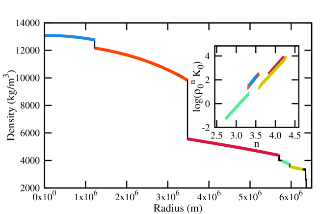
Figure 1: (color online) In black, significantly buried under the theoretical calculations, is the Preliminary Reference Earth Model (Dziewonski & Anderson, 1981) (PREM) and the newer Reference Earth Model (Kustowski et al., 2008) (REF). The colored lines are a sample calculation of ours for inner core (blue), outer core (orange), lower mantle (red), transition (light green) and upper mantle (yellow). There is excellent (less than 1%) disagreement between theory and experiment. The inset depicts the linear range of the polytrope index that share excellent agreement with experimental data using as a legend the same colors as the main plot.

In Fig. 1 we show a density profile of planet Earth from the seismic analysis of the Preliminary Reference Earth Model (Dziewonski & Anderson, 1981) (PREM) and the newer Reference Earth Model (Kustowski et al., 2008) (REF) giving a profile of Earth’s inner core, outer core, and three stages of the mantle. Most of the seismic data is obscured by our calculation of the solution to Eq. (24) using our fixed polytrope assumption. Our calculation returned excellent results for the density profile and the gravitational and pressure profiles as well (not shown) using a variety of different vacuum densities, $\rho_{0}$, bulk moduli, $B_{0}$, and polytrope indices which are equal to the bulk modulus pressure derivative ($\frac{dB_{0}}{dP}\equiv B^{\prime}_{0}\equiv n$). The inner most boundary had its density set at the value from the experimental data set, the first derivative initial value was constrained using Eq. (14) and Eq. (22). The poorest fit was for the liquid outer core but results were still well under 1% error. However the predictive power of this fixed index analysis is weak. With an ideal theory, one would assume that by choosing vacuum values which best fit the experimental seismic data one could elicit more detail about the composite materials comprising the interior Earth. Unfortunately a plethora of values for $\rho_{0},B_{0}$, and $B^{\prime}_{0}$ give excellent simultaneous fits to both the density-radius and the density-pressure profile. The inset of Fig. 1 details this lack of clarity. Each theoretical result which provided a good agreement to the subset seismic data of the interior Earth is provided by a point on a line of the form $\log_{10}(\rho_{0}^{n}K_{0})=m\;n+b$. The polytropic index $n$ worked well over a large range as long as $\rho_{0}$ and $K_{0}$ were constrained to the displayed line. By using an EOS which fixes this polytrope observable means that the best fits will reflect only the best average values of $(\frac{dB}{dP})$ for that span of the interior of the Earth. For example the inner core is best reproduced with a fixed index range of $3.35<n<3.55$ but it is know that at the surface the same materials, rich in iron, will have $n>4.5$ (Seager et al., 2007; Sha & Cohen, 2010; Garai et al., 2011; Yamazaki et al., 2012). Having a fixed polytropic index for planets does not represent the physical reality adequately, despite the fact that the pressure-density and density-radius profiles were described satisfactorily. Unlike the solar models which do have a near constant pressure derivative of the bulk modulus, the planet density-radius models, due to their relatively high compressibility, are rather insensitive to the pressure derivative of the bulk modulus (our newly discovered polytrope index). We will delve further into the analysis of the seismic data for Earth in Sect. 7, but next we advance a variable polytrope procedure which will give our model more physical insight.

4 Making the Polytropic Index a Variable

The ansatz that the polytropic index is constant is constraining and unrealistic. Eddington inherently recognized this with star formation and attempted a variable index analysis (1938). It is well known that for all materials the derivative of the bulk modulus with respect to pressure does change ($\frac{\partial^{2}B}{\partial P^{2}}\neq 0)$ (Zhang et al., 2007; Garai, 2007; Singh, 2010). We show later that the bulk modulus pressure derivative can best be approximated as a constant only at pressures below $10^{9}$ Pa (small rocky planets or asteroids) or above $10^{14}$Pa (interiors of stars and very massive planets). Most planets have a pressure at their core which is between these extremes, including our Earth and all the planets in our solar system. Likewise the Murnaghan EOS was quickly deemed unsatisfactorily because of its constant derivative of the bulk modulus with respect to pressure so Birch proposed an extension (Birch, 1947). A more realistic approach would allow the index to vary while at the same time retaining the definition for the polytrope index, $n=\frac{dB}{dP}$.

4.1 Modifying the Polytrope

So first assuming a modified polytrope with a variable index we must allow for the contingent that the polytrope expression, derived in Sect. 2, is no longer constant

$$\rho^{n(\rho)}K=\rho_{0}^{n(\rho)}K_{0}h(\rho),$$ (25)

where we have introduced a new function, $h(\rho)$ which is a measure of the non-conservation of the fixed expression or a weighting function. In the limit of the fixed case $h(\rho)=1$.

By taking the natural log of this equation and then taking the pressure derivative

$$\frac{d}{dP}\left(n(\rho)\ln\frac{\rho}{\rho_{0}}+\ln\frac{K}{K_{0}}\right)=\frac{d}{dP}\ln h(\rho),$$ (26)

and progressing by realizing that $B=K^{-1}$, $\frac{d}{dP}\ln\rho=K$, and thus $\frac{d}{dP}\ln K=-\frac{dB/dP}{B}$

$$\frac{dn(\rho)}{dP}\ln\frac{\rho}{\rho_{0}}+\frac{n(\rho)}{B}-\frac{dB/dP}{B}=\frac{d}{dP}\ln h(\rho),$$ (27)

We chose to maintain $n=\frac{dB}{dP}$, thus two terms cancel and we have

$$\frac{dn(\rho)}{dP}\ln\frac{\rho}{\rho_{0}}=\frac{d}{dP}\ln h(\rho).$$ (28)

This is a simple prescription on how use a modified polytrope with a variable index equivalent to the pressure derivative of the bulk modulus. We now have a new replacement for compressibility, using Eq. (25) we have

$$K=\frac{\rho_{0}^{n(\rho)}K_{0}h(\rho)}{\rho^{n(\rho)}},$$ (29)

which is analogous to the fixed $n$ version, Eq. (22), with the addition of a weighting function, $h(\rho)$.

4.2 Changes to the Lane-Emden Equation

The new modified Lane-Emden equation, which now includes a variable $n$. Starting with

$$\frac{d^{2}\rho}{dr^{2}}-\left[\frac{2}{\rho}+\frac{K^{\prime}}{K}\right]\left(\frac{d\rho}{dr}\right)^{2}+\frac{2}{r}\frac{d\rho}{dr}+4\pi G\rho^{3}K(\rho)=0,$$

it is trivial to remove $K$ in terms of $\rho$ using Eq. (29). We also need to find $K^{\prime}=\frac{dK}{d\rho}$, which is a larger undertaking since $n$ is no longer constant and needs to be treated with care. Starting again with Eq. (25) we take the logarithm of both sides

$$\frac{d}{d\rho}\log K = \frac{d}{d\rho}(\log h+\log\rho_{0}^{n}K_{0}-n\log\rho)$$ (30)

$$= \frac{d}{d\rho}\log h-\frac{dn}{d\rho}\log\rho-n\frac{d}{d\rho}\log\rho+\frac{dn}{d\rho}\log\rho_{0},$$

recognizing that we can use earlier relationships if we assume a natural log

$$\frac{dK}{d\rho}=K\left(\frac{d\ln h}{d\rho}+\frac{dn}{d\rho}\ln\frac{\rho_{0}}{\rho}-\frac{n}{\rho}\right)$$ (31)

and then using Eq. (28) and the definition $K=\frac{1}{\rho}\frac{d\rho}{dP}$ a cancellation occurs and we are left with the same result as with a fixed $n$

$$\frac{dK}{d\rho}=K^{\prime}=K(-\frac{n}{\rho}),$$ (32)

except now $n$ is no longer a constant but a density dependent function. Thus the only symbolic change to the Lane-Emden equation is in the final term

$$\frac{d^{2}\rho}{dr^{2}}-\left[\frac{2-n(\rho)}{\rho}\right]\left(\frac{d\rho}{dr}\right)^{2}+\frac{2}{r}\frac{d\rho}{dr}+4\pi G\,h(\rho)\,\rho_{0}^{n(\rho)}K_{0}\rho^{3-n(\rho)}=0,$$ (33)

where the function $h(\rho)$ is introduced and $n$, the polytrope index and equivalent to the derivative of the bulk modulus with respect to pressure, is also assumed a function of density as expected. This derivation is independent of the EOS function chosen for $n(\rho)$ which, by Eq. (28), is also intrinsically linked to the weighting function $h(\rho)$.

4.3 Our Equation of State

To have a working hypothesis for a dynamic polytrope index EOS we examined previous equations of state (Roy & Roy, 2005, 2006) and pressure-density relationships (Seager et al., 2007; Swift et al., 2012) for an empirical function form for the changing polytrope index. To be consistent we developed our own EOS which uses the informed polytrope index as the function of reference in place of the more common pressure EOS like the Birch-Murnaghan (Birch, 1947; Poirier, 2000) or Vinet (Vinet et al., 1987, 1989; Poirier, 2000). We found that

$$n(\rho)=\frac{dB}{dP}=A_{0}\left(\frac{\rho_{0}}{\rho}\right)^{A_{1}}+A_{2}$$ (34)

works well (more detail on how this empirical equation was developed is proffered in Sect. 5). It is a respectable EOS for pressures up to the $10^{13}$ Pa range. The resulting functional form for the polytrope index is also exceedingly simple. All other major relations to this polytrope index can be found analytically by integration or differentiation, using fundamental relations found in Appendix B. Specifically applying these relations to our EOS as expressed in Eq. (34) we find for pressure

$$P=\frac{B_{0}e^{\frac{A_{0}}{A_{1}}}}{A_{1}}\left[\left(\frac{\rho}{\rho_{0}}\right)^{A_{2}}E_{n}\left(\frac{A_{1}+A_{2}}{A_{1}},\frac{A_{0}}{A_{1}}\left(\frac{\rho_{0}}{\rho}\right)^{A_{1}}\right)-E_{n}\left(\frac{A_{1}+A_{2}}{A_{1}},\frac{A_{0}}{A_{1}}\right)\right].$$ (35)

This pressure equation contains a special function, the generalized exponential integral ($E_{n}$) which is defined as

$$E_{n}(n,x)=\int_{1}^{\infty}\frac{e^{-xt}}{t^{n}}dt.$$ (36)

The parameters $A_{0},A_{1},A_{2}$ are dimensionless, connected to experiment, and well behaved, always greater than zero and less than ten. They are connected to the extremes of the polytrope index: the infinite pressure derivative of the bulk modulus with respect to pressure,$B^{\prime}_{\infty}=n_{\infty}$ and the zero pressure asymptote of the same observable, $B^{\prime}_{0}=n_{0}$. They were fit as follows: $A_{2}=B^{\prime}_{\infty},A_{0}=B_{0}^{\prime}-A_{2}$, and $A_{1}=\frac{-B_{0}B_{0}^{\prime\prime}}{B_{0}^{\prime}-A_{2}}$. In this work we used the parameter settings in a predictive method, setting $B_{0}$, and $B_{0}^{\prime}$ close to experimental results, choosing a near fixed, but yet to be determined, infinite pressure derivative ($1.75<B^{\prime}_{\infty}<2.1$), and assuming a universal ratio for $B_{0}^{\prime\prime}$ by setting

$$A_{1}=\frac{B_{0}^{\prime}}{B_{0}^{\prime}-A_{2}}\equiv\frac{B_{0}^{\prime}}{A_{0}},$$ (37)

which we borrowed from Roy & Roy (2006). Thus for any given material there are only three parameters ($\rho_{0},B_{0},$ and $B^{\prime}_{0}$). We will show our EOS compared to experiment in subsection 4.5 but first we require that it be continuous with a higher pressure theory to extend its validity.

4.4 Pressures above Ten Tera-Pascal

Inspired by Seager et al. (2007) we went higher in pressure, to $10^{18}$ Pa, by following their technique to match at some critical density our empirical EOS to the Thomas-Fermi-Dirac theory (Salpeter & Zapolsky, 1967) which treats at extreme pressures the quantum mechanic Fermi-Dirac gas whose pressure we approximated as

$$P(\rho)=P_{0}+F_{3}\rho+F_{2}\rho^{4/3}+F_{1}\rho^{5/3}$$ (38)

where

$$F_{1} = \frac{5.16\times 10^{12}Pa}{(2690\frac{A}{Z})^{5/3}}$$

$$F_{2} = \frac{5.16\times 10^{12}Pa}{(2690\frac{A}{Z})^{4/3}}(.40726Z^{2/3}+.20732)$$

$$F_{3} = \frac{5.16\times 10^{12}Pa}{(2690\frac{A}{Z})^{3/3}}(.01407),$$ (39)

the variable $P_{0}$ of Eq. (38) is a small, relatively low pressure, addition to keep pressure continuity across the matching boundary and will be determined last. If the material is not monatomic we use a weighted average for $A$ and $Z$ (atomic and proton number respectively).

Following the common definition used between the pressure and the bulk modulus, $B=\rho\frac{dP}{d\rho}$, we have for this high pressure theory

$$B=(5/3)F_{1}\rho^{5/3}-(4/3)F_{2}\rho^{4/3}-(3/3)F_{3}\rho^{3/3}.$$ (40)

Likewise $n$, our polytrope index equals

$$\frac{dB}{dP}=n=\frac{\rho}{B}\frac{dB}{d\rho},$$ (41)

thus

$$n=\frac{(5/3)^{2}F_{1}-(4/3)^{2}F_{2}\rho^{-1/3}-F_{3}\rho^{-2/3}}{(5/3)F_{1}-(4/3)F_{2}\rho^{-1/3}-F_{3}\rho^{-2/3}}.$$ (42)

A key aspect of this method is to choose the critical density in which to switch from $n(\rho)=A_{0}(\frac{\rho_{0}}{\rho})^{A_{1}}+A_{2}$, to the $n$ of Eq. (42). We found that by requiring at the boundary that the bulk modulus, $B$, was continuous and using the secant method to find this critical density was all that was required. We also found that at this critical density $n$, the derivative of the bulk modulus, also was continuous. By adding a relatively small constant to pressure ($P_{0}$ of Eq. (38)) we can also set the pressures equivalent at the critical density boundary. The reason we get a match between both $B$ and $n$ at the boundary is because these two variables are not independent. Recalling Eq. (41), $\frac{dB}{dp}=n=\frac{\rho}{B}\frac{dB}{d\rho}$, we see that if $\rho$ and $B$ are attuned we get the two derivatives, $n=\frac{dB}{dP}$ and $\frac{dB}{d\rho}$ as bonus. With this extension to a high pressure EOS, we now feel comfortable in fitting up to $10^{18}$ Pa which are core pressures typical of small stars.

Pragmatically we assume informed values for a material’s $\rho_{0},B_{0}$, and $B^{\prime}_{0}$. We then make initial approximations for $A_{2}\approx 2$. We then solve for $A_{0},$ and $A_{1}$ of Eq. (34). Then a secant algorithm adjusts $A_{2}$ and then determines $A_{0},$ and $A_{1}$ so at the critical density, $\rho_{c}$, the low pressure EOS becomes continuous with the higher pressure Thomas-Fermi-Dirac EOS (TFD) of Eq. (40) by finding at what critical density $B_{ours}-B_{TFD}=0$. We then ensure that $n_{ours}-n_{TFD}=0$ and then we lastly solve for $P_{0}$ of Eq. (38) to establish continuity for pressure, bulk modulus, and the pressure derivative of the bulk modulus across the critical boundary. As supplemental material we provide an example code to build a multi-layered planet which has this methodology within (see Sect. 5).

4.5 Comparison with experimental results

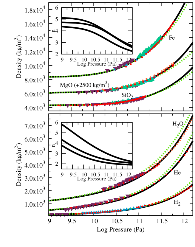
Figure 2: (color online) We describe six materials with our EOS with a solid black line. In the bottom panel an older EOS, the Vinet (Vinet et al., 1987, 1989; Poirier, 2000), is represented by a green dashed line (parameters for H₂ (Loubeyre et al., 1996),parameters for He (Loubeyre et al., 1993),parameters for H₂O (Tkachev & Manghnani, 2000), we modified $B^{\prime}=7.25$, well with in range to give a better fit). In the top panel an older EOS, the Birch-Murnaghan (Birch, 1947; Poirier, 2000), is also represented by a green dashed line (parameters for MgO (Duffy et al., 1995), parameters for SiO₂ (Driver et al., 2010; Ping et al., 2013)), we took an average value between the two references for $B=305$ GPa and $B^{\prime}=5.0$). The iron green dashed line is represented by the Vinet with parameters given by Anderson et al. (2001). More sophisticated first principle EOS (density functional theories) are a red or orange dashed line (H₂-DFT (Geng et al., 2012),He-GGA (Khairallah & Militzer, 2008), H₂O-QMD (red) (French et al., 2009) and H₂O-(orange) (Hermann et al., 2011), MgO-GGA-B1 (red) and qMS-Q ff (orange) (Strachan et al., 1999),SiO₂-DFT (Driver et al., 2010),Fe-EXAFS (Ping et al., 2013)). Experimental data is expressed in purple, blue, and turquoise triangles (H₂-purple (Zha et al., 1993), blue (Geng et al., 2012),He-purple (Cazorla & Boronat, 2008),H₂O-purple (Sugimura et al., 2008), MgO-purple,blue,turquoise (Duffy et al., 1995) SiO₂-purple (Panero et al., 2003b),blue (Xun et al., 2010),Fe-purple, blue, turquoise (Sha & Cohen, 2010)). The MgO curve is offset for aesthetic reasons, so that the calculation does not run into the calculation for SiO₂. The inset shows the changing value of the polytrope index as the pressure changes in our EOS. All the parameters used for our calculation in this plot can be found in Appendix C.

In Fig. 2 we plot density versus pressure for six common materials that make up planet interiors in our solar system ranging from molecular hydrogen to atomic iron. The materials are either solids or liquids throughout the calculation and are also low temperature isothermal calculations (cold curves, 0K - 300K). We choose to examine an intermediate pressure range, $10^{9}$ Pa to $10^{12}$ Pa, because it is challenging; it is at the extreme of our experimental capabilities and the interiors of our solar system planets are in this range. The solid black line of the inset is our EOS which was input into the Lane-Emden equation of Eq. (33) through the polytropic index (as a check of our work we used Eq. (35)). At these lower pressures we used the EOS described with Eq. (34), the values of the parameters can be also found in Appendix C. The filled triangles of various colors are experimental data, the dashed green line is a common empirical theory from the twentieth century (Birch-Murnaghan (Birch, 1947) or Vinet (Vinet et al., 1987, 1989; Poirier, 2000) which begins to fail in the $10^{11}$ Pascal range, the dotted red and orange lines are density functional theories and/or quantum Monte Carlo theories from the twenty-first century. Our theory has the correct general trends, it fits theories and experimental data well considering that it has no adjustable parameters. Our method was that we first chose average experimental values for our material vacuum values of $\rho_{0},B_{0},$ and $n_{0}$. In many cases the literature values varied widely and so some prudence was used to determine the selected values. Our parameter $A_{2}$ was chosen as the critical boundary value for $n=\frac{dB}{dP}$ when the EOS transitioned from our own to the Thomas-Fermi-Dirac EOS (Salpeter & Zapolsky, 1967) ($1.75<A_{2}<2.1$) and we fixed out remaining parameters by constraining $A_{0}+A_{2}=n_{0}$ and $A_{0}A_{1}=n_{0}$. All the parameters used to calculate the pressure-density profiles of Fig. 2 can be found in Appendix C.

This success is proof of concept, that it is possible to develop an experimentally informed EOS which uses a polytrope function form, equivalent to $\frac{dB}{dP}$, which can be naturally and consistently input into the dynamic index Lane-Emden equation. It rivals the popular universal Birch-Murnaghan (Birch, 1947; Poirier, 2000) and Vinet (Vinet et al., 1987, 1989; Poirier, 2000) in predictive potential as it mimics well the high pressure first-principle theories (French et al., 2009; Geng et al., 2012; Khairallah & Militzer, 2008; Hermann et al., 2011; Driver et al., 2010; Ping et al., 2013). The inset of Fig. 2 plots the polytrope index as a function of the same pressure range for the six materials. The polytrope index, $n=\frac{dB}{dP}$ does change significantly over this pressure range, thus to keep the polytrope index fixed for planets in our solar system would be worse than approximate.

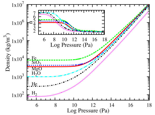
Figure 3: (color online) Our EOS calculation shown over a large pressure range similar to Fig. 2. The inset also has the same form as the inset of Fig. 2, the change in the polytrope index as a function of the same pressure range as the main plot.

Figure 3 shows our calculation over a wider pressure range, with a similar inset as Fig. 2. Note the general trends: up to $10^{7}$ Pa the pressure density profile is a nearly incompressible horizontal line, the polytrope index, equivalent to the pressure derivative of the bulk modulus, wanders little from from its zero pressure value. The most dynamic range of change for the polytrope index is from $10^{8}$ Pa to $10^{14}$ Pa as was illustrated in Fig. 2. As the pressure increases, our theory must switch from the low pressure EOS of Eq. (34) to the technique of Thomas-Fermi-Dirac of Sect. 4.4. The polytrope index again becomes nearly constant after $10^{14}$ Pa as each material begins its slow asymptotic drive towards the Thomas-Fermi-Dirac value of $5/3$ (Salpeter & Zapolsky, 1967). The parameters used for the materials in this figure can be found in Appendix C. A word of caution; since this is a simple universal EOS it will not contain any insight about quantum phase transitions which will take place in many of these materials above $10^{11}$ Pascals.

As one approaches solar pressure range, as we do in Fig. 3 ($>10^{15}Pa$), it is interesting to note that the polytrope index is again near constant. Was Eddington’s choice of the polytrope index set to $4/3$ for main sequence stars (Eddington, 1916) thus fortuitous? Assume, in a main sequence star, the most significant interactions under extreme pressure and temperature are gravity, electron repulsion, and heat flow. Eddington assumed only heat flow and gravity but completely neglected the significant electron repulsion in a dense solar gas yet still calculated satisfactory results. If we examine the derivative of the bulk modulus with respect to pressure, our newly revealed polytrope index, we discover why. For large massive objects like suns their partial bulk moduli with respect to pressure have similar values, greater than one and less than two ($\approx 4/3$ for heat flow (Eddington) and $\approx 5/3$ for electron repulsion if the Thomas-Fermi-Dirac scheme of Salpeter & Zapolsky (1967) is followed). The thermal and electric contribution to the change in the bulk modulus is nearly the same as one follows the pressure gradient. Over ninety percent of a stars interior (all but the near surface) can be described well by a constant polytrope index that averages somewhere between $4/3$ (thermal) and $5/3$ (electrical). As seen in this work the sensitivity of the polytrope index is small enough that this $1/3$ difference has little effect on the final results.

The EOS developed is an unsophisticated example of the power of this variable polytrope method. At its foundation is the equivalency between the polytrope index and the important elastic variable, the pressure derivative of the bulk modulus. Other planet formation methods include a universal electric EOS in interplay with thermal effects (Stacey & Davis, 2004; Valencia et al., 2006; Sotin et al., 2007; Grasset et al., 2009; Leconte & Chabrier, 2012; Swift et al., 2012; Wagner et al., 2012; Zeng & Sasselov, 2013) but they vary in their approach. This technique has as its centerpiece one elastic variable from which all dynamic interactions (electric, thermal, magnetic, nuclear) can contribute and thus one prescription to control input into the differential equations. This EOS has the ability to mature alongside its elastic variable polytrope index as we will discuss further in Sect. 7.

5 Application to Planets

We now apply our method to planets of our solar system. For planets the changing polytrope index is a must for all but the smallest planets. One looming approximation that needs to be addressed is the use of cold isothermal material curves to describe planets with hot interiors. We will address this in Sect. 7, but for now let us proceed assuming that this simplification is feasible.

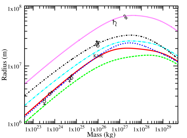
Figure 4: (color online) The legend of the six lines are the same as for Fig. 3, six materials that are common in planetary interiors. The symbols run vertically from top to bottom as Jupiter, Saturn, Uranus and Neptune (on top of each other), Earth and Venus (on top of each other), Mars, and Mercury. The symbol k10c stands for exoplanet Kepler 10c which is a super-earth (Dumusque et al., 2014).

In Fig. 4 we solve the modified Lane-Emden equation with a variable index for the same six materials of the two previous figures except now we plot mass versus radius. This is a popular figure in planet modeling papers dating back to at least Zapolsky & Salpeter (1969). For comparison we designate the positions on the figure for the planets of the solar system. Described from vertical top to bottom: Jupiter, Saturn, Uranus and Neptune (almost on top of each other), Earth and Venus (almost on top of each other), Mars and Mercury. They are all placed close to their line of significant composition. Jupiter is close to hydrogen, Saturn has slightly more helium than Jupiter. Uranus and Neptune are between water and helium, Earth, Venus, Mars are between iron and the silicates. Mercury, the most metallic is closest to iron. These logical results give confidence to the validity of the method. Examining the previous results of Zapolsky and Salpeter (1969) and Seager et. al (2007) we have very similar results where the radius hits a maximum for all materials at a mass somewhere between one thousandth and one hundredth of a solar mass. This is not entirely surprising since all three studies used at extreme high densities the theory found in Salpeter & Zapolsky (1967). Our variable polytropic model does add additional physical insight into this maximum. It is well known that the traditional polytrope has a fixed radius for the $n=2$ case (Chandrasekhar, 1939), the radius grows with mass for fixed $n>2$ and the radius shrinks with mass for fixed $n<2$. This maximum of Fig. 4 represents the variable polytrope analog to this fixed radius case. All maximum of Fig. 4 occur within a small range, $1.78<n(\rho)<1.92$. At the same time this result shows little correlation with the vacuum density ($\rho_{0}$), bulk modulus ($B_{0}$), and pressure derivative of the bulk modulus ($n_{0}$) for all six materials. The importance of the $n\approx 2$ range is also evident by examining the change of sign in the second term of Eq. (33) which is our final version of the variable polytrope Lane-Emden equation. The general trends of Fig. 4 also validate the conclusions of Valencia et al. (2007b) which put maximum radial limits on rocky planets thus making it possible to separate the ice giants from the rocky giants. For an exoplanet super-earth example we put Kepler 10c also on Fig. 4 (labeled ’k10c’). This planet is the mass of Neptune, extremely hot at the core, and very dense (Dumusque et al., 2014), our temperature independent theory still places the planet in the correct bulk composition range.

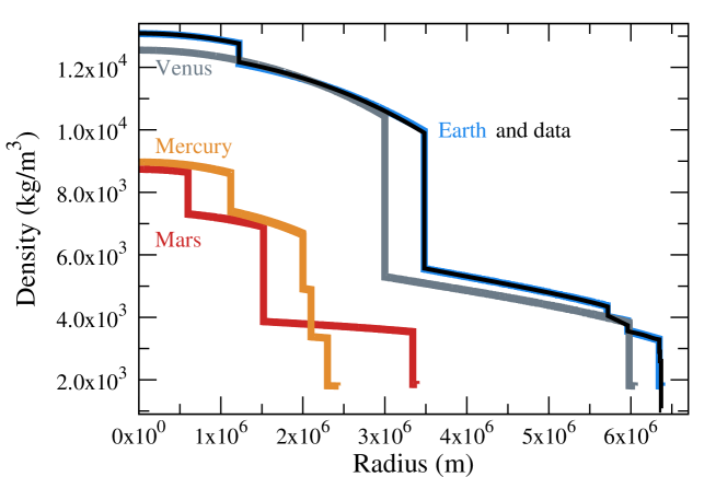
Figure 5: (color online) Mercury, Venus, Earth, and Mars density-radius profile predictions using our EOS. The newer Reference Earth Model (Kustowski et al., 2008) seismic data is plotted as a black line. The details of construction are in the text.

Turning now to specific models for the four rocky planets in our solar system. We constrain the boundary interfaces of these multi-layered planets by substituting for the compressibility, $K$, in Eq. (29) our variable index assumption

$$K=\frac{\rho_{0}^{n(\rho)}K_{0}h(\rho)}{\rho^{n(\rho)}}.$$

Using Eq. (14), we are then left with a constraint on the derivative at each boundary

$$\frac{d\rho}{dr}=-\frac{\rho_{0}^{n(\rho)}\;K_{0}\;h(\rho)}{\rho(r)^{n(\rho)-2}}\;g(r).$$ (43)

The method of construction is illustrative. We assume the material makeup of the layers and the size of each layer, we then also assume the core pressure. There are no further adjustable parameters. The materials dictate the parameters in the equations of state, the core pressure determines the starting core density (by using Eq. (35)), and the interface constraint defines the density values and their first derivatives at the boundaries uniquely, the program runs from the core ($r=0$) to the surface solving the differential equation of Eq. (33) and using the EOS as summarized in Eq. (34). Numerically this differential equation is very stable and solvable with relative ease, there are no variables that gave us numerical difficulty. Table 1 contains our pertinent values for these multi-layer constructions. The materials at each layer are picked by consulting the best ’general knowledge’ about each of the layers and estimating their average density, bulk modulus, etc. Since the rocky planets are relatively small the significance of $A_{mean}$ and $Z_{mean}$ is minimal since their dependence stems from the extremely high pressure theory (see subsection 4.4 for more detail). The method is a standardized way to put a multi-layered planet together. As supplemental material we include our code for the calculation of Earth (Variable PolyPy), written in Python.

In Fig. 5 we plot these hypothetical density-radius profiles for the four rocky planets. In Table 2 we have displayed the results for mass, radius, mean density, and gravity at the surface. For all three models the theoretical results are within a percent of experimental values. This technique provides a systematic method to build mult-layered planets. One of the benefits of using this method is that the EOS has its foundation in the elastic bulk modulus and its pressure derivative. We believe this is an asset that can be utilized to develop EOSs of greater sophistication, we study this question in the next section.

	$\rho_{0}$	$B_{0}$	$n_{0}$	$A_{mean}$	$Z_{mean}$	thickness	$P_{C}$
	$kg/m^{3}$	$GPa$				$m$	$GPa$
Mercury
core 1	7700	180	5.0	55	26	$1.12E6$	$4.04E1$
core 2	6410	132	4.9	55	26	$8.80E5$	$2.67E1$
core 3	4800	220	4.8	44	21	$1.00E5$	$5.63E0$
mantle	3320	200	4.1	36	18	$2.00E5$	$3.63E0$
crust	1800	160	4.0	30	15	$1.36E5$	$0.94E0$
Venus
core	7475	160	4.95	47	22	$3.00E6$	$2.95E2$
mantle	3800	190	4.0	36	18	$2.98E6$	$1.22E2$
crust	1800	170	4.2	30	15	$7.11E4$	$1.14E0$
Earth
core 1	7550	171	5.0	55	26	$1.22E6$	$3.64E2$
core 2	6830	140	5.0	55	26	$2.26E6$	$3.29E2$
mantle 1	3950	190	4.4	36	18	$2.23E6$	$1.36E2$
mantle 2	3650	205	4.1	36	18	$2.51E5$	$2.36E1$
mantle 3	3270	135	3.8	36	18	$3.84E5$	$1.37E1$
crust	1800	160	4.0	30	15	$3.72E4$	$0.66E0$
Mars
core 1	7500	180	5.0	55	26	$6.00E5$	$4.04E1$
core 2	6100	130	4.9	47	22	$9.20E5$	$3.66E1$
mantle	3530	200	4.2	36	18	$1.82E6$	$2.20E1$
crust	1850	160	4.1	30	15	$5.10E4$	$0.35E0$

Table 1: Mars in two steps, Jupiter and Uranus in three steps. The variables $\rho_{0},B_{0}$, and $n_{0}$ would be the values of those observables at zero vacuum. Thickness is the radial size of the core or mantle part, $P_{C}$ is the assumed pressure at the largest depth for each layer.

	mass	radius	mean density	surf. gravity
	$kg$	$m$	$kg/m^{3}$	$m/s^{2}$
Mercury
calculation	$3.29E23$	$2.44E6$	$5.43E3$	3.70
experiment	$3.30E23$	$2.44E6$	$5.43E3$	3.70
Venus
calculation	$4.83E24$	$6.05E6$	$5.20E3$	8.80
experiment	$4.87E24$	$6.05E6$	$5.24E3$	8.87
Earth
calculation	$5.98E24$	$6.38E6$	$5.49E3$	9.80
experiment	$5.97E24$	$6.37E6$	$5.51E3$	9.80
Mars
calculation	$6.38E23$	$3.39E6$	$3.91E3$	3.71
experiment	$6.42E23$	$3.39E6$	$3.93E3$	3.71

Table 2: The rocky planets of our solar system observable predictions using our EOS. The experimental results are taken from the National Aeronautics and Space Administration website.

6 Using the pressure derivative of the bulk modulus as the Equation of State Foundation

The role of the pressure derivative of the bulk modulus ($B^{\prime}\equiv\frac{dB}{dP}$), which we have shown to be the polytrope index, $n$, has grown in importance in material science science (Birch, 1947; Keane, 1954; Vinet et al., 1987, 1989; Poirier, 2000; Roy & Roy, 2005, 2006). As strain theory continued to progress this elastic observable assumed a more prominent role. It is, frankly, a wonderful observable. It is dimensionless, of order one (for all materials and pressures), and because it is proportional to the second derivative of pressure-density it has tremendous sensitivity. This work has developed a robust technique where the variable polytrope index is equivalent to this elastic observable, $B^{\prime}$.

6.1 The importance of $\frac{dB}{dP}$ in material research

Stacey (2000) developed an EOS that used $B^{\prime}\equiv\frac{dB}{dP}=n$ as the starting point. This work gives a thorough history of this technique and rightly recognizes Murnaghan (1944) and Keane (1954) as instrumental in the development of the Stacey EOS. Stacey and Davis strongly believe that $B^{\prime}$ should be the center-piece of a universal EOS (Stacey & Davis, 2004, 2008a; Lal et al., 2009; Singh & Dwivedi, 2012).

Calculating from first principles the electronic contribution to the bulk modulus is well established in the literature (Ravindran et al., 1998). The ability for modern material theorists to develop excellent $B^{\prime}$ theories from density functional theory is not in doubt (Zhang et al. (2010) for example). There have also been some recent high pressure models which include temperature as a direct extension of the pressure equation (Sotin et al., 2007; Wagner et al., 2011, 2012). Our calculation technique would use alternative methods which show the thermodynamic connection between $B^{\prime}$, the Grüneisen parameter (Stacey & Davis, 2004, 2008a; Shanker et al., 2009) and temperature (Stacey & Davis, 2004, 2008b), Sotin et al. (2007) gives a good overview of both techniques. The elastic constants, such as $B^{\prime}$, are a natural environment to develop temperature dependence as shown in a variety of research at low pressures (Zhang et al., 2007), first principle calculations of copper (Narasimhan & de Gironcoli, 2002), magnesium oxide (Li et al., 2005) or high pressure iron (Sha & Cohen, 2010) and high pressure salt (Singh, 2010). We will examine this potential by adding a primitive temperature dependence in Sect. 7. Phase changes would also have a natural place in a foundational $B^{\prime}$ EOS. The discontinuities created by phase changes would be more significant in the bulk modulus and its derivative than in a pressure-density curve. The importance of magnetic effects has also recently been studied (Pourovskii et al., 2013) and similarly the $B^{\prime}$ equation has been shown to be a natural place to add this interaction (Zhang et al., 2010). Classical solid state theory may also be of use. The intermediate polytrope expression we derived in the context of the fixed polytrope index, $\rho^{n}K=h(\rho)\rho_{0}^{n}K_{0}$ (Eq. (25)) in Sect. 4, has some remarkable similarities to the functional form of the repulsive coulomb potential informed by Born-Madelung theory (Kittel, 2005).

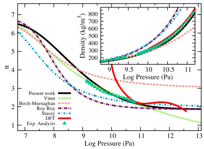
Figure 6: (color online) A plot of $n\equiv\frac{dB}{dB}$ for cold-curve molecular hydrogen using a variety of EOSs. The solid black line is the present calculation, the green dotted line is the EOS of Vinet (Vinet et al., 1987, 1989), the pink dashed line is the third order EOS of Birch-Murnaghan Birch (1947). We also present the EOS of Stacey 2000 (blue dash - dot fixing the infinite $\frac{dB}{dP}$ at 2) and the EOS of Roy-Roy (Roy & Roy, 2001; Roy & Roy, 1999) is depicted by a purple long dash - dot. A recent density functional theory (DFT) developed for molecular hydrogen (Geng et al., 2012) in red. All EOS (except the DFT) have fixed $\rho_{0}=79.43kg/m^{3}$, $B_{0}=0.162GPa$. The $n_{0}$ values are within 3% of each other (ours, Birch-Murnaghan is $n=6.7$, Vinet is $n=6.813$ and we have set Roy-Roy and Stacey to $n=6.9$). Note the dramatic differences in the function $n(P)$ and its effects on the density-pressure relationship at extreme pressures. The experimental analysis, in blue triangles, was done by taking 2nd derivatives of experiments done by Loubeyre et al. (1996)

6.2 Comparisons of $\frac{dB}{dP}$

As stated in Sect. 4 we found that

$$n(\rho)=\frac{dB}{dP}=B^{\prime}=A_{0}\left(\frac{\rho_{0}}{\rho}\right)^{A_{1}}+A_{2}$$

works well. It is a respectable EOS for pressures up to $10^{13}$ Pa and it can be extended to higher pressures by attaching it to quantum mechanical models as also discussed in Sect. 4. This EOS was cultivated by examining the functional form of $\frac{dB}{dP}$ for the Vinet and Birch-Murnaghan EOS (Birch, 1947; Poirier, 2000) and also analyzing pressure-density relationships found in previous work (Roy & Roy, 2005, 2006; Seager et al., 2007; Swift et al., 2012) including first principle calculations (French et al., 2009; Hermann et al., 2011; Geng et al., 2012) and acquired numerical second derivatives. This was instrumental in developing the intermediate pressure ranges ($10^{11}-10^{13}Pa$) which older EOS often do not fit well. Our result is entirely empirical but it meets the criteria that it is using $B^{\prime}$ as its foundation, that it is analytically simple, and that it strives to go at least an order of magnitude higher than the earlier EOSs.

The analysis included taking analytical second derivatives of EOSs using

$$B = \rho\frac{dP}{d\rho}$$

$$n = \frac{dB}{dP}=B^{\prime}=\frac{d}{dP}\left(\rho\frac{dP}{d\rho}\right)$$ (44)

$$\mbox{so }\frac{dB}{B}=\frac{n}{\rho}d\rho.$$

The analytical results for the Vinet, Birch-Murnaghan (Birch, 1947; Poirier, 2000), Stacey (2000),  Roy & Roy (1999), and an EOS for hydrogen derived from density functional theory (Geng et al., 2012) are shown for completeness in Appendix D, these results are non-trivial fractions. One of the goals of this work was to develop a analytical formula for $\frac{dB}{dP}$ which is simpler than the two most used universal equations, the Vinet and Birch-Murnaghan, yet at the same time mimic their behavior.

We portray $\frac{dB}{dP}$ in Fig. 6 for molecular hydrogen as a function of pressure for a variety of EOSs and in the inset we show the pressure-density result. This figure is similar to Figs. 2 and 3 but now the focus is on the behavior of the polytrope index so the plot proper and inset have been switched. We choose hydrogen because it offers challenges at relatively low pressures because of its high compressibility. It was seen in Fig. 2 that a standard Vinet EOS does not do well as one approaches pressures of $10^{13}Pa$, and Fig. 6 gives the probable cause, the Vinet becomes soft as it heads towards a lower asymptote for $n$ than any of the other EOSs do. In contrast, the complete failure of the Birch-Murnaghan EOS with these chosen parameters is because the asymptote for $n$ is higher than the rest of the EOSs. All the EOSs (except the DFT by Geng et al. (2012) which is valid in a limited range only) approach a constant at extreme pressures but they disagree at what the infinite pressure constant ($B^{\prime}_{\infty}$) should be. Analysis of the importance of this asymptote is examined in good detail in the research of Stacey and Davis (Stacey, 2000; Stacey & Davis, 2004, 2008a). The Birch-Murnaghan, in Fig. 6, has the highest $B^{\prime}_{\infty}$ of $3$. The Vinet has the lowest, $B^{\prime}_{\infty}=2/3$, the rest are $5/3\leq B^{\prime}_{\infty}\leq 2$. Our theory, because it connects to the Thomas-Fermi-Dirac high pressure theory has as its asymptote $B^{\prime}_{\infty}=5/3$, we set Stacey’s EOS to $B^{\prime}_{\infty}=2$ (they treat it as an adjustable parameter).

Note the peculiarity of the density function theory (Geng et al., 2012). The authors choose a pressure EOS (see Appendix D) which fit only the pressures applicable to their theory ($1\times 10^{10}$ Pa to $4\times 10^{12}$ Pa). When derivatives are taken to produce $\frac{dB}{dP}$ the results are complicated and quickly unstable at the extremes (the ends of the plotted curve head towards infinity). This insensitivity provides an additional lesson on how it is easy to fit the density-pressure results and yet have faulty derivatives, an authoritative EOS will fit the pressure-density, bulk modulus-density and bulk modulus pressure derivative and density profiles.

The experimental density-pressure profile comes from Loubeyre et al. (1996). The technique we used to analyze this data to produce the polytrope index, as depicted in Fig. 6, is detailed in Appendix D. To summarize, we fit a density-pressure curve to a high order polynomial and then take two derivatives, using Eqs. 44, to achieve a good analysis independently, directly from the data, of $n\equiv\frac{dB}{dP}$. We urge that this technique be used by experimentalists to further analyze their high precision data. With a good experimental set of density-pressure data one can also determine the bulk modulus and the pressure derivative of the bulk modulus over the same range. If one does want to extrapolate to vacuum pressure using a universal EOS, this information will help produce an authoritative EOS and further constrain the parameters chosen. A similar technique and conclusion was proffered by Ziambaras & Schröder (2003).

It has been argued by Stacey & Davis (2004) that $B^{\prime}_{\infty}>5/3$ but not necessarily $B^{\prime}_{\infty}=5/3$. The argument is that phase changes and proton number dependence make it difficult to rectify that all materials will approach the same asymptote. We also believe this is an open question but still found it convenient to set it to the Thomas-Fermi-Dirac value of $5/3$ (Salpeter & Zapolsky, 1967). Yet we recognize that the present work and others (Seager et al., 2007) have found that this asymptote is not reached quickly. With the additional insight that the polytrope index is the derivative with respect to pressure of the bulk modulus we look at the interior of stars for guidance. All stars, at the core, have an index $<2$. All stars are under extreme electronic, nuclear, and thermal pressure, thus indicating that the contributions to $B^{\prime}$ from these sources are all under 2 in the extreme pressure limit.

Too often the universal EOSs are used to put limits on the bulk modulus and its derivative at zero pressure ($B_{0},B^{\prime}_{0}$). All reasonable EOSs will fit any pressure-density curve if the parameters are adjusted enough as discussed in  Stacey & Davis (2004), what Fig. 6 shows is the disparity that exists between the EOSs on the functional form and the asymptote of $\frac{dB}{dP}$. This observable needs to be measured or analyzed experimentally as well as theoretical approaches from first principles (Ziambaras & Schröder, 2003). The observable should be ascertained independent of any universal EOS so the best functional forms can be developed. Molecular hydrogen, helium, and water, because of their higher compressibilities, are a good place to start. These informed results would catalyze the development of EOSs. With a trusted functional form, which mimics experiment for pressure-density, bulk modulus-density, and especially $B^{\prime}$-density (which is sensitive even at low pressures), there will be more faith in the physical interpretation of the parameters being adjusted. To constrain the universal functional form beyond the pressure-density profile would have significant impact on calculations of larger planets. In the next section we use these objectives on fitting Earth using our EOS.

7 Analysis of planet Earth with our EOS

The Earth is our best pseudo-static laboratory for studying materials under high pressures. In this section we analyze the Earth using different constraints on our EOS to better elucidate its strengths and weaknesses.

By using the seismic data of planet Earth we now constrain, with our EOS, the material of the inner core, outer core and mantle using the pressure-density profile, and the density-radius profile. The best results still achieve an excellent fit and reveal a linear analysis similar to the inset of Fig. 1, ($\rho_{0}^{n_{0}}K_{0}$ vs. $n_{0}$) An example calculation was shown in Fig. 5 and the code which produced this calculation is included as supplementary material. The linear equations for the inner core, outer core, and lower mantle of the Earth are as follows:
inner core: $\log_{10}(\rho_{0}^{n_{0}}K_{0})=3.994n_{0}-11.813$
outer core: $\log_{10}(\rho_{0}^{n_{0}}K_{0})=3.977n_{0}-11.836$
lower mantle: $\log_{10}(\rho_{0}^{n_{0}}K_{0})=3.702n_{0}-11.717$
A reminder that the linear analysis constrains $\rho_{0}^{n_{0}}K_{0}$ but does not guarantee that every point on the line will be a good fit, but all good fits are very near that line. We offer no explanation for this relationship but that its success does speak to the validity of universal EOSs and that the three variables ($\rho_{0},K_{0},n_{0}$) are not independent. An oversimplification in our technique is that the experimental material fits were all to cold curves, we will address this assumption in the next subsection.

7.1 Temperature Analysis

Seager et al. (2007) have argued that temperature dependencies are significant but manageable (less than 10% in a pressure-density profile). We agree and the reasonable physical observables predicted in Fig. 4 and Fig. 5 for the rocky planets exemplify the power of using approximate cold curves. By using the seismic data of planet Earth we may now, with our equation of state, constrain further the material of the inner core, outer core and mantle and examine the role of temperature dependence for our EOS.

As one moves from the surface of a planet to its core the polytropic index, $\frac{dB}{dP}$, moves from close to its vacuum value to a lower value. The effect of temperature is to slow this descent as one immerses into the hotter interior in an approximately adiabatic path. For all of our calculations above, which were cold curves, we fixed the product and sum of our parameters to $A_{0}+A_{2}=n_{0}$ and $A_{0}A_{1}=n_{0}$. The sum is required for all curves, the product was a fortuitous choice suggested by Roy-Roy (2006) which worked well for cold curves, it controls the relative size of the second derivative

$$\frac{dn}{d\rho}=-A_{0}A_{1}\frac{\rho_{0}^{A_{1}}}{\rho^{A_{1}+1}}$$ (45)

(see appendix B for more detail). The cold curves $A_{2}$ was set by a numerical secant search that connected our cold curve EOS to the Thomas-Fermi-Dirac EOS, the values for $A_{2}$ was always between 1.75 and 2.1. So by increasing the value of $A_{2}$ we decrease the magnitude of this derivative thus providing a simple method to include temperature. The procedure is simple: assume a reasonable material with a given vacuum density ($\rho_{0}$), bulk modulus ($B_{0}$), and first pressure derivative of the bulk modulus($n_{0}$). The constraints on $A_{0},A_{1},$ and $A_{2}$ are that $n_{0}=A_{0}+A_{2}$ and $n_{0}=A_{0}A_{1}$. We treat as free parameters $\rho_{0},B_{0},n_{0}$ and $A_{2}$ and adjust them using a Powell method (constraining $A_{0}$ and $A_{1}$ by $A_{0}+A_{2}=A_{0}A_{1}=n_{0}$). So we are assuming that at the surface of the Earth (vacuum pressure) the density, bulk modulus, first derivative with respect to pressure, and all higher order derivatives have the same value irregardless of whether the isothermal or adiabatic path is chosen. But as one moves into the interior $B_{adiab}>B_{isotherm}$ thus the elastic derivatives are also disparate. In Stacey & Davis (2004, 2008b) one finds a thermodynamic derivation that provide a mapping

$$B_{adiab}=B_{isothermal}(1+\gamma\alpha\Delta T),$$ (46)

where $\gamma$ is the Grüneisen parameter and $\alpha$ is the volume expansion coefficient (which are related to the bulk modulus and its pressure derivative). The reference temperature for $\Delta T$ is low, the temperature at the surface of the Earth. This ratio of $B_{adiab}$ over $B_{isothermal}$ remains close to normal, in Stacey & Davis (2004) it never goes above 1.10 for planet Earth. This is a substantial piece of evidence that the isothermal cold curves are a good approximation for the interior of the Earth.

As $B_{adiab}$ increases faster than $B_{isothermal}$ as the pressure increases, this implies directly that $n_{adiab}\equiv\frac{dB_{adiab}}{dP}>\frac{dB_{isotherm}}{dP}\equiv n_{isotherm}$ Pragmatically this is not too difficult, we must have an $A_{2}$ greater than the cold isothermal curves ($>2.2$) and so we vary $\rho_{0},B_{0},n_{0}$ and $A_{2}$ to fit the interior of the Earth. This fitting has only one more adjustable parameter,$A_{2}$, than the cold isothermal curves. We will label this primitive temperature dependent method ’model VII’, after the section from which it was introduced.

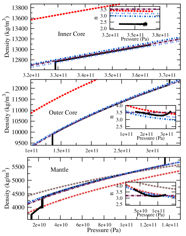
Figure 7: (color online) This figure is in three panels: the top referencing the inner core, the middle the outer core, and the bottom is the inner mantle. In black, significantly buried under the theoretical calculations, is the newer Reference Earth Model (Kustowski et al., 2008) (REF). The colored lines are all calculations of ours with different sophistication, all parameters are given in Table 3. The three models are named from the section from which they were introduced. Model (VII – two light blue short dashed) includes an adjustable second derivative ($\frac{d^{2}B}{dP^{2}}$) to simulate the effect of temperature in the interior of the Earth. Model (IV - short dark blue dashed-dot) is the same material as (1) but the second derivative functional form has now been fixed to the cold curve value effectively removing the temperature dependence. Model (III – purple long dash-dot) is the least sophisticated fixed polytrope index (($\frac{d^{2}B}{dP^{2}}=0$). For reference the cold curve for hcp iron is included for the cores (dashed red) and magnesium oxide (dashed pink) and silicon dioxide (dashed brown) is included for the mantle. The inset contains a depiction of the function $n(P)\equiv\frac{dB}{dP}(P)$ for our three models along with experimental analysis direct from the seismic wave data of the newer Reference Earth Model (Kustowski et al., 2008) (REF) depicted by the thick black line.

In Fig. 7 we examine the inner core, outer core and mantle of the Earth in more detail than Fig. 1 and Fig. 5. We begin by plotting the seismic results, as we did in Fig. 1, except now we plot the pressure-density profile (sold black line). Since the data sets are large and precise they are informative. Not only do they contain the pressure-density but they also implicitly contain the derivatives. Here we calculate the bulk modulus directly from the $s$ and $p$ wave velocities (see Stacey & Davis (2004) for example) and we then calculate the pressure derivative of the bulk modulus numerically which is represented by the black line on the inset. We also plot three models from this work (named after the section number from which they were introduced): a good fit using the fixed polytrope index from Sect. 3 (model III,$\frac{d^{2}B}{dP^{2}}\equiv 0$, purple horizontal line), a good fit using a variable polytrope index from this section (temperature dependent, model VII, light blue dashed line), and the same material as model VII with the temperature dependence removed, thus a isothermal cold curve as described in Sect. 4 (model IV, dark blue dashed line). For reference we also plot, from Sect. 4, the cold curves for iron, silicon dioxide, and magnesium oxide at those pressures. Model VII was fit simultaneously to the density-pressure curve (main graph), the bulk modulus, the density-radius curve (Fig. 1) and the pressure derivative of the bulk modulus-pressure curve (inset). This last constraint, depicted in the inset, shows the wonderful dynamics that are exhibited within the interior of the Earth. The outer core and mantle do not adhere to the monotonically decreasing pressure derivative of the bulk modulus of our cold curve or primitive temperature models but as the layer boundary approaches the second pressure derivative of the bulk modulus changes sign (the material’s rate of hardness growth increases!) as surmised by the analysis of the seismic data. The mantle and outer core have shown to be wonderful examples of phase-changes, non-adiabatic regions, and convection (Alboussière et al., 2010; Katsura et al., 2010; Matyska et al., 2011) as the seismic waves slow as they near these boundary layers. The simple form of our EOS cannot describe this dynamic and so we hope only to stay close. Luckily the sensitivity to the pressure derivative is manageable. This polytrope method forces the user to contemplate beyond the density-pressure profiles to constraining the derivatives thus making it an ideal tool for bulk composition studies in the interior of a rich dynamic planet.

Our simple temperature dependence does an adequate job describing the changing polytrope index for the mantle and the outer core, especially away from the inner boundary layer. The direction is correct, the magnitude is of the right order for the thermal pressure and the bulk modulus differential of Eq. (46) ($B_{adiab}/B_{isothemal}\approx 1.01$ for the mantle and $\approx 1.04$ for the outer core). Most importantly we can describe the functional form of the polytrope index adequately. The inner core has the right direction and magnitude also ($B_{adiab}/B_{isothemal}\approx 1.04$ for the inner core) but we fail to find an adequate function to match the low experimental analysis of the interior polytrope index($n\approx 2.3$!). The most obvious potential source of error is that the functional form of our temperature dependence does not have the complexity to adequately describe the adiabatic curve relative to the cold temperature curve at inner core pressures. Recent experimental research (Tateno et al., 2010; Anzellini et al., 2013) also indicates the presence of a phase change near the geothermal which a universal EOS cannot describe. We also could easily be missing important magnetic (Pourovskii et al., 2013) or rotational effects. Again this method naturally extends the variables open to sensitivity examination thus providing a systematic tool to examine the successes and failures of any chosen EOS. We do have some faith in our estimation for $n_{0}$ of the core because we do match the bulk modulus number at the core to a good precision.

Model	$\rho_{0}$	$B_{0}$	$n_{0}$	$A_{0}$	$A_{1}$	$A_{2}$
from Sect.	$[kg/m^{3}]$	$GPa$
Earth Inner Core
Sect. VII	7563.0	196.39	4.486	1.736	2.584	2.750
Sect. IV	7563.0	196.39	4.486	2.369	1.893	2.117
Sect. III	7372.6	194.74	3.525	0.0	-	3.525
Fe	8300.0	165.0	5.150	3.080	1.672	2.070
Earth Outer Core
Sect. VII	6654.2	131.32	4.748	2.096	2.266	2.652
Sect. IV	6654.2	131.32	4.748	2.652	1.791	2.096
Sect. III	6596.7	153.33	3.500	0.0	-	3.500
Earth Mantle
Sect. VII	3988.4	207.30	4.104	1.804	2.275	2.300
Sect. IV	3988.4	207.30	4.104	2.199	1.867	1.905
Sect. III	3942.9	216.85	3.200	0.0	-	3.200
MgO	3580.0	157.0	4.371	2.465	1.772	1.904
SiO2	4287.0	305.0	4.750	2.983	1.592	1.767

Table 3: $\rho_{0},B_{0},n_{0}$ are chosen to be a good fit to the models of the Earth based on experiment. Model (VII - two dashed light blue on Fig. 7) is the most realistic allowing the parameters $A_{0}$ and $A_{1}$ to vary to simulate temperature dependence. Model (IV - dark blue short dash-dot on Fig. 7) is the same material with the temperature dependence removed and thus not as good fit. The simplest model (III - purple long dash-dot on Fig. 7) is a fixed polytrope index. The fixed polytrope does not require the sophistication of the earlier models but it can still be reduced to a specific case of the variable model by setting $A_{0}=0,A_{2}=n$ and noting that it is independent of $A_{1}$. For reference we depict the cold curve prediction for $\epsilon$-iron in the core panels, we add magnesium oxide and silicon dioxide for the mantle.

The results of the three models are systematically logical. For the best fit with realistic values for the vacuum density, bulk modulus, and pressure derivative of the bulk modulus the adiabatic curve version with an unsophisticated temperature dependence, model VII, had good success as the listings show in Table 3 and depicted in Fig. 7. This result implies that this technique has the potential to add temperature and any other dynamic variables if the effect of these variables on $\frac{dB}{dP}$ are known (profiles). Even with our simple adiabatic temperature model we were able to fit the density-radius profile to $<$ 2%, the density-pressure profile to $<$ 1%, the bulk modulus of the core to $<$ 3%, and the pressure derivative of the bulk modulus for the outer core and mantle to $<$ 10%, the inner core we fit to 30%.

Recognizing that choosing our EOS as authoritative (the best functional forms for the cold curves) is a source of possible systematic error (when our EOS errs it is likely to error on the hard side as depicted by Fig. 6) as is our simple model for adiabatic temperature dependence (the slope of the polytrope index-pressure curve is low for mantle and outer core), we choose to constrain the interior of the Earth materials with conservative, fair errors:
inner core: $\rho_{0}=7600\pm 300kg/m^{3}$, $B_{0}=190\pm 40GPa$, and $B_{0}^{\prime}=4.7\pm 0.5$
outer core: $\rho_{0}=6800\pm 300kg/m^{3}$, $B_{0}=130\pm 30GPa$, and $B_{0}^{\prime}=4.8\pm 0.3$
mantle: $\rho_{0}=4100\pm 200kg/m^{3}$, $B_{0}=200\pm 30GPa$, and $B_{0}^{\prime}=4.2\pm 0.3\;$ .
The constant $\rho_{0}^{n_{0}}K_{0}$, which plays a pivotal role in this research, explains why the bulk modulus is difficult to constrain. This constant is extremely sensitive to the compressibility and its inverse, the bulk modulus. A small change in $\rho$ or $n$ will cause a much larger change in the bulk modulus if this term is to stay near constant.

If the effects of temperature and other dynamic variables are not specified explicitly then a reasonable material cold curve can be used instead and the error will be very manageable, less than 5% for a rocky planet like Earth as detailed in the analysis of the ratio of Eq. (46) which we always found to be under 1.05 using our primitive temperature dependence model. This trend is further bolstered by examining the difference between the density-pressure curves of Fig. 7. So we recommend the use of cold curves, with reasonable material observables, as a very good approximation for the actual geothermal path that describes the rocky planet under study. However we do not recommend the reverse analysis of trying to fit only the pressure-density experimental data with a cold curve to elucidate the the vacuum elastic variables the results will also be suspect and highly dependent on the EOS used.

By numerically analyzing the experimental seismic data we have constrained our EOS further than most (fitting to pressure-density, density-radius, bulk modulus-pressure and $\frac{dB}{dP}$ vs. pressure) and can thus eliminate many previous parameter choices. We have also added a primitive temperature dependence which has the correct direction and the right order of magnitude. So we felt confident, with our model VII, to constrain the materials in the interior of the Earth with moderation. For better analysis we would need a reasonable temperature, magnetic, phase-change and convection profile, prepared from first principles, which would more tightly constrain the parameters.

7.2 Summary of Technique

The method presented here is systematic, builds on history, and is able to grow in complexity as the EOS becomes more complex. To summarize this theoretical apparatus to solve the radius-density profile for a multi-layered planet:

• Develop a functional form or differential equation(s) for the polytrope index as a function of density. The dynamic variables that describe this polytrope index function can be sophisticated and include a full thermal, electromagnetic, and nuclear profile: $n(\rho)\equiv\frac{dB(\rho)}{dP}$ for an appropriate core material with a given $\rho_{0},B_{0},B_{0}^{\prime}\equiv n_{0}$ and core pressure.

• Solve analytically or numerically for the weighting function:$\ln h(\rho)=\int_{\rho_{0}}^{\rho}\frac{dn}{d\rho}\ln(\frac{\rho}{rho_{0}})\;d\rho$

• Starting at the inner core ($r=0$) find the core density using the weighting function $h(\rho)$ and core pressure relationship, also set $\frac{d\rho}{dr}=0$.

• Solve the Lane-Emden differential equation (Eq. (33)) to a chosen radius (or if the surface, when $\rho(r)=\rho_{0}$).

• If another layer is desired choose an appropriate material with a given $\rho_{0},B_{0},B_{0}^{\prime}$ then calculating $n(\rho)$ and $h(\rho)$ as shown above.

• Choose an initial density for the next layer and a starting radius ($r=r_{final}$ of the previous layer).

• Find the initial derivative, $\frac{d\rho}{dr}$ by using Eq. (43) and Eq. (33).

• Solve the differential equation to a chosen radius (or if the surface, when $\rho(r)=\rho_{0}$). Repeat the last 4 steps if additional layers are desired.

If one uses a series of differential equations and profiles which produce numerical functions only for the polytrope index, $n(\rho)$, it would be preferred to start at the surface of the planet and work inward since the calculus relations will also not be analytical. This would involve some more computational challenges, but they are not insurmountable as Zeng & Seager (2008) have demonstrated.

8 Summary and Conclusion

In summary this work derived a variable polytrope approach. To investigate the method we also developed a new universal EOS which is distinctive because it is a function of the polytrope index. This work first exhumed, in Sect. 2, that the historic polytrope index is for all cases and materials equivalent to the derivative with respect to pressure of the bulk modulus ($n=\frac{dB}{dP}$). This result is the foundation of the article, the further development that follows is inspired and motivated by recognizing the physical implications of the polytropic index as an elastic constant thus giving it a life beyond merely index status. We solve the Lane-Emden differential equation for plausible solutions to the density profile of the five layer interior of the Earth. We find that there is a wide range of constant polytropic indexes ($n=\frac{dB}{dP}$) that agree with the seismic data of the interior of the Earth.

In Sect. 4 we expand our technique by making the polytropic index a variable. Since the index has been shown to be equivalent to the derivative with respect to pressure of the bulk modulus ($n=\frac{dB}{dP}$) this is a natural progression since all materials have a decreasing first derivative along the isotherm when the pressures become very large. We re-derive the Lane-Emden differential equation for a variable polytropic index in a consistent manner. We then introduce an empirically developed functional form for our variable polytropic index, $n(\rho)=A_{0}(\frac{\rho_{0}}{\rho})^{A_{1}}+A_{2}$, which is our submission for a isothermal universal equation of state. With this creation we can create analytical formulas for pressure and bulk modulus as a function of density. We, more importantly, use our variable polytropic index as input in the Lane-Emden differential equation, we are able to make pressure-density profiles for six materials which are common in the interior of planets which compare favorably to experiment. By connecting our results to high pressure theory (Salpeter & Zapolsky, 1967) we are able to make theoretical calculations up to $10^{18}Pa$. We turn to the planets of our solar system in Sect. 5 where we show that their masses and radii compare favorably with mass-radius curves for the six common materials. We then show that this technique can be applied to a multi-layered body as we fit our technique to the rocky planets.

In Sect. 6 and Sect. 7 we discuss the importance of developing a universal EOS from $\frac{dB}{dP}$, we then compare our functional form for $\frac{dB}{dP}$ to previous work and to experimental analysis. The importance of constraining a EOS fit beyond the mundane pressure-density profile is demonstrated. We show that our EOS has the advantage of being simple and thus easy to grow in sophistication. One addition that is needed is the adding of temperature dependence, we do this in primitive form and show a variety of results using the interior of the Earth as our laboratory. We also verify earlier work that shows that temperature modification is a relatively small effect, under 5% or the Earth’s density-pressure profile. Finally using a variety of experimental analysis, we are able to narrow the constituent vacuum densities of the Earth to 5%, the bulk moduli to 20%, and the pressure derivative of the bulk moduli to 10%.

Having revealed the polytrope index as the pressure derivative of the bulk modulus is fortuitous for future research advancement. There are many first principle EOS theories (density functional, quantum Monte-Carlo) which calculate the pressure derivative of the bulk modulus (Ravindran et al., 1998; Sha & Cohen, 2010; Xun et al., 2010; Li et al., 2005). The prominence of the bulk modulus in this procedure may also lends itself to solid state Born-Madelung calculations (Kittel, 2005). By using the modified polytrope assumption of this work one also has a straight forward procedure to solve the Lane-Emden equation for planets and stars using more sophisticated equations of state. These methods may include dynamic convective interactions, heat flow, rotational dynamics, magnetic kinetics, and nuclear reactions which would all contribute to the overall pressure derivative of the bulk modulus, the variable polytrope index, complementing a new generation of realistic planetary and solar models. We hope that this technique strengthens the relevance of the polytrope method for planet and solar research and continues what Lane, Eddington, and Chandrasekhar began a century ago.

Appendix A Relations between density and Compressibility from the Murnaghan EOS

It was Stacey and Davis 2004; 2008a who we have seen state that in the context of the Murnaghan EOS the relationship

$$\frac{B}{B_{0}}=(\frac{\rho}{\rho_{0}})^{B_{0}^{\prime}},$$ (47)

which is equivalent to our own intermediate results for the fixed polytrope index (Eqs.(4,5)). The derivation of Eq. (47) is straightforward but we include it in some detail because the relation is used extensively in this work.

Assuming only a linear change in the bulk modulus

$$B=B_{0}+B_{0}^{\prime}P,$$ (48)

where $B_{0}^{\prime}$ is the fixed derivative with respect to pressure. One can then insert the definition of the bulk modulus

$$\rho\frac{dP}{d\rho}=B_{0}+B_{0}^{\prime}P,$$ (49)

and integrating and describing the zero pressure boundary conditions by using a naught subscript, one gets

$$\frac{\ln(B=B_{0}+B_{0}^{\prime}P)}{B_{0}^{\prime}}=\ln\frac{\rho}{\rho_{0}}+\frac{\ln B_{0}}{B_{0}^{\prime}}$$ (50)

which reduces to

$$(1+\frac{B_{0}^{\prime}P}{B_{0}})=(\frac{\rho}{\rho_{0}})^{B_{0}^{\prime}}.$$ (51)

Finally using Eq.(48) to substitute $B_{0}^{\prime}P=B-B_{0}$ we have the desired relation, Eq. (47).

The Murnaghan EOS is found by solving Eq. (51) for pressure

$$P=\frac{B_{0}}{B_{0}^{\prime}}\left((\frac{\rho}{\rho_{0}})^{B_{0}^{\prime}}-1\right).$$ (52)

The similarity of this equation to the polytrope is undeniable

Appendix B Our Empirical Equation of State

We developed an equation of state from analysis of earlier empirical equations of state. The major difference is ours uses the polytrope index, the pressure derivative of the bulk modulus, as its place of development. It was first stated in the text proper as Eq. (34), again

$$n(\rho)=\frac{dB}{dP}=A_{0}\left(\frac{\rho_{0}}{\rho}\right)^{A_{1}}+A_{2}.$$

The constants are chosen as follows: $A_{2}\rightarrow B^{\prime}_{\infty}$ (approximately 1.95 or connecting it to the results of Salpeter & Zapolsky (1967)), $A_{0}=B_{0}^{\prime}-A_{2}$, and $A_{1}=\frac{-B_{0}B_{0}^{\prime\prime}}{B_{0}^{\prime}-A_{2}}$ where $B^{\prime}_{\infty}$ is the asymptotic value at very high densities, see Appendix C for more details In this work we set $B_{0}$, and $B_{0}^{\prime}$ to experimental results and assume a universal ratio for $B_{0}^{\prime\prime}$ by setting

$$A_{1}=\frac{B_{0}^{\prime}}{B_{0}^{\prime}-A_{2}}=\frac{B_{0}^{\prime}}{A_{0}},$$ (53)

which we borrowed from Roy-Roy (2006). Now using these fundamental relations

$$B = \rho\frac{dP}{d\rho}$$ (54)

$$n = \frac{dB}{dP}=\frac{d}{dP}\left(\rho\frac{dP}{d\rho}\right)$$ (56)

$$\mbox{so }\frac{dB}{B}=\frac{n}{\rho}d\rho$$

$$\ln h = n\ln\frac{\rho}{\rho_{0}}+\ln\frac{B_{0}}{B}$$ (57)

in conjunction with Eq. (28)

$$\frac{dn(\rho)}{dP}\ln\frac{\rho}{\rho_{0}}=\frac{d}{dP}\ln h(\rho).$$

It can thus be shown

$$\frac{dh}{h}=\ln\frac{\rho}{\rho_{0}}\frac{dn}{d\rho}\>d\rho.$$ (58)

Specifically applying these relations to our EOS as expressed in Eq. (34) we find

$$n = \frac{dB}{dP}=A_{0}\left(\frac{\rho_{0}}{\rho}\right)^{A_{1}}+A_{2}$$ (59)

$$B = B_{0}e^{M(\rho)}\left(\frac{\rho}{\rho_{0}}\right)^{A_{2}}$$ (60)

$$P = \frac{B_{0}e^{\frac{A_{0}}{A_{1}}}}{A_{1}}\left[\left(\frac{\rho}{\rho_{0}}\right)^{A_{2}}E_{n}\left(\frac{A_{1}+A_{2}}{A_{1}},\frac{A_{0}}{A_{1}}\left(\frac{\rho_{0}}{\rho}\right)^{A_{1}}\right)-E_{n}\left(\frac{A_{1}+A_{2}}{A_{1}},\frac{A_{0}}{A_{1}}\right)\right]$$ (61)

$$\frac{dn}{dP} = \frac{d^{2}B}{dP^{2}}=-A_{1}\frac{(\frac{dB}{dP}-A_{2})}{B}$$ (62)

$$\ln h = \frac{A_{0}}{A_{1}}\left(\frac{\rho_{0}}{\rho}\right)^{A_{1}}\left(1+A_{1}\ln\frac{\rho}{\rho_{0}}\right)-\frac{A_{0}}{A_{1}}$$ (63)

$$h = e^{-M(\rho)}\left(\frac{\rho}{\rho_{0}}\right)^{A_{0}{(\frac{\rho_{0}}{\rho})^{A_{1}}}},$$ (64)

noting that only $n(\rho)$ and $h(\rho)$ are needed to solve the Lane-Emden differential equation, Eq. (33). The functions in the exponents are given by

$$M(\rho)=\frac{A_{0}}{A_{1}}(1-(\frac{\rho_{0}}{\rho})^{A_{1}})\\$$

The only equation which is non-analytical is pressure which contains a special integral function, the generalized exponential integral ($E_{n}$) which is defined as

$$E_{n}(n,x)=\int_{1}^{\infty}\frac{e^{-xt}}{t^{n}}dt.$$ (65)

By using the assumption of Ref. (Roy & Roy, 2006), we are equating the second derivative as

$$B_{0}^{\prime\prime}=-\frac{B_{0}^{\prime}}{B_{0}}.$$ (66)

This is true at the surface but we can find the general relation also for our EOS. First taking the derivative of the polytrope index with respect to density,

$$\frac{dn}{d\rho}=-A_{0}A_{1}\frac{\rho_{0}^{A_{1}}}{\rho^{A_{1}+1}}$$ (67)

then switching variables to a pressure derivative we have

$$\frac{dn}{dP}=-A_{0}A_{1}\frac{\rho_{0}^{A_{1}}}{\rho^{A_{1}+1}}\frac{d\rho}{dP}=-A_{0}A_{1}\frac{\rho_{0}^{A_{1}}}{B\rho^{A_{1}}}=-A_{1}\frac{(\frac{dB}{dP}-A_{2})}{B}.$$ (68)

By doing a substitution for $A_{1}$ in terms of $A_{2}$ (using Eq. (53)) in Eq. (68) we have finally

$$\frac{dn}{dP}=\frac{d^{2}B}{dP^{2}}=-(\frac{B_{0}^{\prime}}{B_{0}^{\prime}-A_{2}})\frac{(\frac{dB}{dP}-A_{2})}{B},$$ (69)

which has an interesting symmetry. This relationship for the second derivative has been studied in some detail recently in Singh & Dwivedi (2012).

Appendix C Parameters chosen for materials

In the text proper we used six materials commonly found in the interior of planets in our solar system. For completeness and reproducibility we include our parameters for the lower pressures ($<10^{13}$ Pa) in Table 4.

material	$\rho_{0}$	$B_{0}$	$n_{0}$	$A_{0}$	$A_{1}$	$A_{2}$
	$[kg/m^{3}]$	$GPa$
H2	79.43	0.162	6.70	4.837	1.385	1.863
He	291.73	0.224	7.15	5.141	1.391	2.009
H2O	998.0	2.20	7.13	5.248	1.359	1.882
MgO	3580.0	157.0	4.37	2.465	1.772	1.904
SiO2	4287.0	305.0	4.75	2.983	1.592	1.767
Fe	8300.0	165.0	5.15	3.080	1.672	2.070

Table 4: $\rho_{0},B_{0},n_{0}$ are chosen to be a rough consensus of the experimental values at vacuum pressure. The values of $A_{0},A_{1},A_{2}$ follow the prescription of Eq. (70) which is slightly adjusted on each iteration of the secant method searching for the critical density. First order approximate values are $A_{2}=1.95$,$A_{1}=\frac{n_{0}}{n_{0}-1.95}$ and $A_{0}=n_{0}-A_{2}$ where $n_{0}={\frac{dB}{dP}}_{0}=B_{0}^{\prime}.$

The parameters, $\rho_{0},B_{0}$, and $n_{0}=\frac{dB}{dP}$, were not adjusted and were set to values which best reflect the experimental results (Zha et al., 1993; Khairallah & Militzer, 2008; Sha & Cohen, 2010; Duffy et al., 1995; Panero et al., 2003a; Driver et al., 2010) the rest of these parameters are derived from these three experimental values. To first approximation these parameters are $A_{2}=1.95$,$A_{1}=\frac{n_{0}}{n_{0}-1.95}$ (or adjustable for best fit) and $A_{0}=n_{0}-A_{2}$ if one needs pressures only up to the Tera-Pascal range.

At higher pressures we switch to a Thomas-Fermi-Dirac scheme of Ref. (Salpeter & Zapolsky, 1967). To make this transformation we find a critical density where we match $B$ and $\frac{dB}{dP}=n$, we then create a match with pressure by adding a constant $P_{0}$ to the Thomas-Fermi-Dirac scheme. We first assume an initial guess using a secant method to find the critical density. The density is than iterated until it meets the requirement $B_{TFD}(\rho_{c})-B_{classical}(\rho_{c})=0$. At this critical density the derivative of the bulk modulus with respect to pressure also matches thanks to the relationship in Eq. (41). At each iteration of the search we adjust $A_{2}$ and then we are able to set $A_{0}$ and $A_{1}$:

$$A_{2} = n_{TFD}-(n_{0}-n_{TFD})*(\rho_{0}/\rho_{c})^{\frac{n_{0}}{n_{0}-n_{TFD}}}$$

$$A_{1} = \frac{n_{0}}{n_{0}-A_{2}}$$

$$A_{0} = n_{0}-A_{2},$$ (70)

where $n_{TFD}$ is the past iterative guess using the present iteration of $\rho_{c}$ in Eq. (42) while $n_{0}$ is set to the rough experimental consensus value. The results of the secant method with additional useful parameters (atomic number, $A$, and proton number, $Z$) are in Table 5.

material	$\rho_{c}$	$B_{c}$	$n_{c}$	$P_{c}$	$P_{0}$	$A$	$Z$
	$kg/m^{3}$	$GPa$		$GPa$	$GPa$
H2	$1.690E4$	$1.154E5$	1.866	$6.165E4$	$2.782E3$	2	2
He	$1.229E4$	$1.623E4$	2.037	$7.801E3$	$7.806E2$	4	2
H2O	$3.758E5$	$7.360E6$	1.883	$3.900E6$	$2.027E5$	18	10
MgO	$1.262E6$	$4.478E7$	1.905	$2.351E7$	$1.434E6$	40	20
SiO2	$1.577E7$	$3.967E9$	1.767	$2.245E9$	$4.396E7$	60	30
Fe	$9.736E5$	$1.998E7$	2.071	$9.631E6$	$1.2806E6$	55.85	26

Table 5: The critical values are found by solving for the critical density, $\rho_{c}$, using the secant method when the bulk modulus of our EOS, Eq. (63) matches the bulk modulus of the degenerative Fermi gas bulk modulus of Thomas-Fermi-Dirac, Eq. (40). The parameters $P_{c}$ and $P_{0}$ are found by forcing the pressure formula of Eq. (40) to equal the pressure formula listed in Eq. (66) by choosing an appropriate $P_{0}$

Again no adjustable parameters are in this table, they were found using the secant method by requiring that the bulk modulus matches at the boundary between the low pressure and high pressure theories.

Appendix D The polytrope index for various equations of state

Our Equation of state is developed from a functional form of $\frac{dB}{dP}$ which is detailed in Appendix B. We repeat them here:

$$B^{\prime}\equiv n = \frac{dB}{dP}=A_{0}\left(\frac{\rho_{0}}{\rho}\right)^{A_{1}}+A_{2}$$ (71)

$$B = B_{0}e^{\frac{A_{0}}{A_{1}}(1-(\frac{\rho_{0}}{\rho})^{A_{1}})}\left(\frac{\rho}{\rho_{0}}\right)^{A_{2}}$$ (72)

$$P = \frac{B_{0}e^{\frac{A_{0}}{A_{1}}}}{A_{1}}\left[\left(\frac{\rho}{\rho_{0}}\right)^{A_{2}}E_{n}\left(\frac{A_{1}+A_{2}}{A_{1}},\frac{A_{0}}{A_{1}}\left(\frac{\rho_{0}}{\rho}\right)^{A_{1}}\right)-E_{n}\left(\frac{A_{1}+A_{2}}{A_{1}},\frac{A_{0}}{A_{1}}\right)\right]$$ (73)

The equation of state of Stacey also starts with $B^{\prime}=\frac{dB}{dP}$,

$$\frac{1}{B^{\prime}}=\frac{1}{B^{\prime}_{0}}+\left(1-\frac{B^{\prime}_{\infty}}{B^{\prime}_{0}}\right)\frac{P}{B}$$ (74)

which then one can derive a formula for the bulk modulus and the density ratio

$$B = B_{0}{\left(1-B^{\prime}_{\infty}\frac{P}{B}\right)}^{-\frac{B^{\prime}_{0}}{B^{\prime}_{\infty}}}$$ (75)

$$\ln\frac{\rho}{\rho_{0}} = -\frac{B^{\prime}_{0}}{{B^{\prime}_{\infty}}^{2}}\ln{\left(1-B^{\prime}_{\infty}\frac{P}{B}\right)}-\left(\frac{B^{\prime}_{0}}{{B^{\prime}_{\infty}}}-1\right)\frac{P}{B}$$ (76)

Most equations of state start from a definition of pressure, one can calculate $n=\frac{dB}{dP}$ from $P(\rho)$ analytically

$$\frac{dB}{dP}=\frac{d}{dP}(\rho\frac{dP}{d\rho})=\rho\frac{dB/d\rho}{B}$$ (77)

Many of the next equations use $\eta=\frac{\rho}{\rho_{0}}=\frac{V_{0}}{V}$. The Vinet EOS (Vinet et al., 1987, 1989; Poirier, 2000) is

$$P = 3B_{0}\eta^{\frac{2}{3}}\left(1-\eta^{-\frac{1}{3}}\right)\exp(\frac{3}{2}(B_{0}^{\prime}-1)(1-\eta^{-\frac{1}{3}}))$$ (78)

$$B = 3B_{0}\left(\frac{2}{3}\eta^{\frac{2}{3}}-\frac{1}{3}\eta^{\frac{1}{3}}+\frac{1}{2}(B_{0}^{\prime}-1)(\eta^{\frac{1}{3}}-1)\right)\exp(\frac{3}{2}(B_{0}^{\prime}-1)(1-\eta^{-\frac{1}{3}}))$$ (79)

$$B^{\prime} = \frac{(\frac{2}{3})^{2}\eta^{\frac{2}{3}}-(\frac{1}{3})^{2}\eta^{\frac{1}{3}}+\frac{1}{2}(B_{0}^{\prime}-1)(\eta^{\frac{1}{3}}-\frac{1}{3})+\frac{1}{4}(B_{0}^{\prime}-1)^{2}(1-\eta^{-\frac{1}{3}})}{\frac{2}{3}\eta^{\frac{2}{3}}-\frac{1}{3}\eta^{\frac{1}{3}}+\frac{1}{2}(B_{0}^{\prime}-1)(\eta^{\frac{1}{3}}-1)}$$ (80)

The Birch-Murnaghan third order EOS is (Birch, 1947; Poirier, 2000)

$$P = \frac{3}{2}B_{0}(\eta^{\frac{7}{3}}-\eta^{\frac{5}{3}})\left(1+\frac{3}{4}(B_{0}^{\prime}-4)(\eta^{\frac{2}{3}}-1)\right)$$ (81)

$$B = \frac{3}{2}B_{0}\left(\frac{7}{3}\eta^{\frac{7}{3}}-\frac{5}{3}\eta^{\frac{5}{3}}+\frac{3}{4}(B_{0}^{\prime}-4)\left(\frac{9}{3}\eta^{\frac{9}{3}}-2(\frac{7}{3})\eta^{\frac{7}{3}}+\frac{5}{3}\eta^{\frac{5}{3}}\right)\right)$$ (82)

$$B^{\prime} = \frac{(\frac{7}{3})^{2}\eta^{\frac{7}{3}}-(\frac{5}{3})^{2}\eta^{\frac{5}{3}}+\frac{3}{4}(B_{0}^{\prime}-4)\left((\frac{9}{3})^{2}\eta^{\frac{9}{3}}-2(\frac{7}{3})^{2}\eta^{\frac{7}{3}}+(\frac{5}{3})^{2}\eta^{\frac{5}{3}}\right)}{\frac{7}{3}\eta^{\frac{7}{3}}-\frac{5}{3}\eta^{\frac{5}{3}}+\frac{3}{4}(B_{0}^{\prime}-4)\left(\frac{9}{3}\eta^{\frac{9}{3}}-2(\frac{7}{3})\eta^{\frac{7}{3}}+\frac{5}{3}\eta^{\frac{5}{3}}\right)}$$ (83)

One must be careful with the Roy-Roy equation of state, they have two different forms. The one they consider superior (Roy & Roy, 1999, 2006, 2005), which has a logarithmic form, does not have a physical $B^{\prime}_{\infty}$ asymptote (it is designed to go no higher than $10^{12}$ Pa). The one we depict in Fig. 6 and Appendix D has a physical asymptotic form and has $B^{\prime}_{\infty}=5/3$ (Roy & Roy, 2001; Roy & Roy, 1999).

The  Roy & Roy (1999) EOS is

$$\eta = 1+aP(1+bP)^{c}$$ (84)

$$B = \frac{aP+abP^{2}+(1+bP)^{1-c}}{a+ab(1+c)P}$$ (85)

$$B^{\prime} = \frac{abc(1+bP)^{-c}(-b(1+c)P-2)+a^{2}(1+bP(b(1+c)P+2))}{(a+ab(1+c)P)^{2}}$$ (86)

where

$$a = \frac{1}{B_{0}}$$ (87)

$$b = \frac{1+2B_{0}^{\prime}-5(B_{0}^{\prime})^{2}-1}{6B_{0}(1-B_{0}^{\prime})}$$ (88)

$$c = \frac{(3(1-B_{0}^{\prime})^{2})}{2B_{0}^{\prime}-5(B_{0}^{\prime})^{2}-1}$$ (89)

The DFT EOS equation of state (Geng et al., 2012) is

$$P = 10^{N(\rho)}$$ (90)

$$B = -\frac{10^{N(\rho)}(a_{1}\rho^{4/3}+2a_{2}\rho+3a_{3}\rho^{2/3}+4a_{4}\rho^{1/3}+5a_{5})\ln(10)}{3\rho^{5/3}}$$ (91)

$$B^{\prime} = \frac{-25a_{5}^{2}\ln(10)-25a_{5}\rho^{5/3}+40a_{4}a_{5}\rho^{1/3}\ln(10)+30a_{3}a_{5}\rho^{2/3}\ln(10)}{15a_{5}\rho^{5/3}+12a_{4}\rho^{6/3}+9a_{3}\rho^{7/3}+6a_{2}\rho^{8/3}+3a_{1}\rho^{9/3}}$$ (92)

$$+ \frac{20a_{2}a_{5}\rho\ln(10)+5a_{1}a_{5}\rho^{4/3}\ln(100)}{15a_{5}\rho^{5/3}+12a_{4}\rho^{6/3}+9a_{3}\rho^{7/3}+6a_{2}\rho^{8/3}+3a_{1}\rho^{9/3}}$$

$$- \frac{16a_{4}^{2}\rho^{2/3}\ln(10)+9a_{3}\rho^{7/3}+4a_{2}\rho^{8/3}+a_{1}\rho^{9/3}+\rho^{4/3}(3a_{3}+2a_{2}\rho^{1/3}+a_{1}\rho^{2/3})^{2}\ln(10)}{15a_{5}\rho^{5/3}+12a_{4}\rho^{6/3}+9a_{3}\rho^{7/3}+6a_{2}\rho^{8/3}+3a_{1}\rho^{9/3}}$$

$$- \frac{16a_{4}\rho^{6/3}+24a_{3}a_{4}\rho^{3/3}\ln(10)+8a_{4}a_{1}\rho^{5/3}\ln(10)+8a_{4}a_{2}\rho^{4/3}\ln(100)}{15a_{5}\rho^{5/3}+12a_{4}\rho^{6/3}+9a_{3}\rho^{7/3}+6a_{2}\rho^{8/3}+3a_{1}\rho^{9/3}}$$

with $a_{0}=1.0683,a_{1}=19.1824(2696^{1/3}),a_{2}=-36.3776(2696^{2/3}),a_{3}=28.5165(2696^{3/3}),a_{4}=-10.6068(2696^{4/3}),a_{5}=1.5224(2696^{5/3})$. These complicated functions were calculated using Mathematica. The power functions are

$$N(\rho)=9+a_{0}+\frac{a_{1}}{\rho^{1/3}}+\frac{a_{2}}{\rho^{2/3}}+\frac{a_{3}}{\rho^{3/3}}+\frac{a_{4}}{\rho^{4/3}}+\frac{a_{5}}{\rho^{5/3}}\\$$ (93)

In Fig. 6 we also attempted to analyze experimental data independent of a universal EOS. We take high precision pressure-density data that enters the $10^{9}$Pa range for light elements and the $10^{10}$Pa range for heavier elements. It is also advantageous to have at least two points of low pressure data ($<10^{8}$Pa) that anchors the fit towards the correct origin. In the case of the hydrogen data we found that a 5th order polynomial gave a very low chi-squared. Once we have a polynomial for $P$, calculating the bulk modulus and the polytrope index are trivial.

$$P(GPa) = a_{0}+a_{1}\rho+a_{2}\rho^{2}+a_{3}\rho^{3}+a_{4}\rho^{4}+a_{5}\rho^{5}$$ (94)

$$B(GPa) = a_{1}\rho+2a_{2}\rho^{2}+3a_{3}\rho^{3}+4a_{4}\rho^{4}+5a_{5}\rho^{5}$$ (95)

$$n = \frac{a_{1}\rho+4a_{2}\rho^{2}+9a_{3}\rho^{3}+16a_{4}\rho^{4}+25a_{5}\rho^{5}}{a_{1}\rho+2a_{2}\rho^{2}+3a_{3}\rho^{3}+4a_{4}\rho^{4}+5a_{5}\rho^{5}}$$ (96)

with $a_{0}=2.26603GPa$, $a_{1}=-4.52911\times 10^{-2}GPa/(kg/m^{3})^{1}$, $a_{2}=2.16832\times 10^{-4}GPa/(kg/m^{3})^{2}$, $a_{3}=1.77254\times 10^{-8}GPa/(kg/m^{3})^{3}$, $a_{4}=1.64780\times 10^{-10}GPa/(kg/m^{3})^{4}$, $a_{5}=-1.48451\times 10^{-13}GPa/(kg/m^{3})^{5}$. It also helps to normalize the fitting routine, have as your dependent fitting variable $\rho/(2\rho_{max})$ so that your domain is much less than one, the range should also be small, here we fit it to Giga Pascals.

References

- Alboussière et al. (2010) Alboussière T., Deguen R., Melzani M., 2010, Nature, 466, 744
- Alibert (2014) Alibert Y., 2014, Astron. Astrophys., 561, A41
- Anderson et al. (2001) Anderson O. L., Dubrovinsky L., Saxena S. K., LeBihan T., 2001, Geophys. Res. Lett., 28, 399
- Anzellini et al. (2013) Anzellini S., Dewaele A., Mezouar M., Loubeyre P., Morard G., 2013, Science, 340, 464
- Birch (1947) Birch F., 1947, Physical Review, 71, 809
- Cazorla & Boronat (2008) Cazorla C., Boronat J., 2008, J. Phys.: Condensed Matter, 20, 015223
- Chandrasekhar (1931) Chandrasekhar S., 1931, ApJ, 74, 81
- Chandrasekhar (1939) Chandrasekhar S., 1939, An Introduction To The Study of Stellar Structure. Dover Publications
- Christians (2012) Christians J., 2012, International Journal of Mechanical Engineering Education, 40, 53
- Driver et al. (2010) Driver K. P., Cohen R. E., Wu Z., Militzer B., Ríos P. L., Towler M. D., Needs R. J., Wilkins J. W., 2010, Proceedings of the National Academy of Sciences, 107, 9519
- Duffy et al. (1995) Duffy T. S., Hemley R. J., Mao H.-k., 1995, Phys. Rev. Lett., 74, 1371
- Dumusque et al. (2014) Dumusque X., et al., 2014, The Astrophysical Journal, 789, 154
- Dziewonski & Anderson (1981) Dziewonski A., Anderson D., 1981, Phys.Earth Planet.Interiors, 25, 297
- Eddington (1916) Eddington A. S., 1916, Mon. Not. R. Astron. Soc., 77, 16
- Eddington (1938) Eddington A. S., 1938, Mon. Not. R. Astron. Soc., 99, 4
- Eggleton & Cannon (1991) Eggleton P. P., Cannon R. C., 1991, ApJ, 383, 757
- Françoise Roques (2015) Françoise Roques O. d. P., 2015, ExoSolar Planets Encyclopedia, http://exoplanet.eu
- French et al. (2009) French M., Mattsson T. R., Nettelmann N., Redmer R., 2009, Phys. Rev. B, 79, 054107
- Garai (2007) Garai J., 2007, Journal of Applied Physics, 102,
- Garai et al. (2011) Garai J., Chen J., Telekes G., 2011, American Mineralogist, 96, 828
- Geng et al. (2012) Geng H. Y., Hong S. X., Li J. F., Wu Q., 2012, J. Appl. Phys., p. 063510
- Grasset et al. (2009) Grasset O., Schneider J., Sotin C., 2009, ApJ, 693, 722
- Hermann et al. (2011) Hermann A., Ashcroft N. W., Hoffmann R., 2011, Proceedings of the National Academy of Sciences
- Horedt (2004) Horedt G., 2004, Polytropes Applications in Astrophysics and Related Fields. Kluwer Acasemic Publishers
- Katsura et al. (2010) Katsura T., Yoneda A., Yamazaki D., Yoshino T., Ito E., 2010, Physics of the Earth and Planetary Interiors, 183, 212
- Keane (1954) Keane A., 1954, Aust. J. Phys., 7, 322
- Khairallah & Militzer (2008) Khairallah S. A., Militzer B., 2008, Phys. Rev. Lett., 101, 106407
- Kittel (2005) Kittel C., 2005, Introduction to Solid State Physics, 8 edn. Wiley, Hoboken, NJ, pp 47–87
- Kustowski et al. (2008) Kustowski B., Ekström G., Dziewoński A. M., 2008, J. Geophys. Res., 113
- Lal et al. (2009) Lal K., Singh C. P., Chauhan R. S., 2009, Indian J. Pure & Ap. Phys., 47, 28
- Lattimer & Prakash (2001) Lattimer J., Prakash M., 2001, ApJ, 550, 426
- Leconte & Chabrier (2012) Leconte J., Chabrier G., 2012, Astron. Astrophys., 540, A20
- Li et al. (2005) Li H., Xu L., Liu C.-Q., 2005, Journal of Geophysical Research (Solid Earth), 110, 5203
- Loubeyre et al. (1993) Loubeyre P., LeToullec R., Pinceaux J. P., Mao H. K., Hu J., Hemley R. J., 1993, Phys. Rev. Lett., 71, 2272
- Loubeyre et al. (1996) Loubeyre P., Letoullec R., Hausermann D., Hanfland M., Hemley R. J., Mao H. K., Finger L. W., 1996, Nature, 383, 702
- Matyska et al. (2011) Matyska C., Yuen D. A., Wentzcovitch R. M., Čížková H., 2011, Physics of the Earth and Planetary Interiors, 188, 1
- Murnaghan (1944) Murnaghan F. D., 1944, Proceedings of the National Academy of Sciences, 30, 244
- Narasimhan & de Gironcoli (2002) Narasimhan S., de Gironcoli S., 2002, Phys. Rev. B, 65, 064302
- Panero et al. (2003a) Panero W. R., Benedetti L. R., Jeanloz R., 2003a, J. Geophys. Res.: Solid Earth, 108, ECV 10
- Panero et al. (2003b) Panero W. R., Benedetti L. R., Jeanloz R., 2003b, J. Geophys. Res.: Solid Earth, 108, ECV 5
- Ping et al. (2013) Ping Y., et al., 2013, Phys. Rev. Lett., 111, 065501
- Poirier (2000) Poirier J.-P., 2000, Introduction to the physics of the Earth’s Interior. Cambridge University Press
- Pourovskii et al. (2013) Pourovskii L. V., Miyake T., Simak S. I., Ruban A. V., Dubrovinsky L., Abrikosov I. A., 2013, Phys. Rev. B, 87, 115130
- Ravindran et al. (1998) Ravindran P., Fast L., Korzhavyi P., Johansson B., Wills J., Eriksson O., 1998, Journal of Applied Physics, 84, 4891
- Roy & Roy (1999) Roy S. B., Roy P. B., 1999, J. Phys.: Condensed Matter, 11, 10375
- Roy & Roy (2001) Roy B., Roy B., 2001, physica status solidi (b), 226, 125
- Roy & Roy (2005) Roy P. B., Roy S. B., 2005, J. Phys.: Condensed Matter, 17, 6193
- Roy & Roy (2006) Roy P. B., Roy S. B., 2006, J. Phys.: Condensed Matter, 18, 10481
- Salpeter & Zapolsky (1967) Salpeter E., Zapolsky H., 1967, Phys.Rev., 158, 876
- Seager et al. (2007) Seager S., Kuchner M., Hier-Majumder C., Militzer B., 2007, ApJ, 669, 1279
- Sha & Cohen (2010) Sha X., Cohen R. E., 2010, Phys. Rev. B, 81, 094105
- Shanker et al. (2009) Shanker J., Singh B. P., Jitendra K., 2009, Condensed Matter Phys., 12, 205
- Singh (2010) Singh P. K., 2010, Indian J. Pure & Ap. Phys., 48, 403
- Singh & Dwivedi (2012) Singh P. K., Dwivedi A., 2012, Indian J. Pure & Ap. Phys., 50, 734
- Sotin et al. (2007) Sotin C., Grasset O., Mocquet A., 2007, Icarus, 191, 337
- Stacey (2000) Stacey F. D., 2000, Geophys. J. Int., 143, 621
- Stacey & Davis (2004) Stacey F. D., Davis P., 2004, Phys. Earth Planet Inter., 142, 137
- Stacey & Davis (2008a) Stacey F. D., Davis P., 2008a, Physics of the Earth, 4 edn. Cambridge University Press, New York, NY, pp 294–313
- Stacey & Davis (2008b) Stacey F. D., Davis P., 2008b, Physics of the Earth, 4 edn. Cambridge University Press, New York, NY, pp 314–336
- Stevenson (1991) Stevenson D. J., 1991, Ann. Rev. of Astron. Astrophys., 29, 163
- Strachan et al. (1999) Strachan A., Cagin T., Goddard W. A., 1999, Phys. Rev. B, 60, 15084
- Sugimura et al. (2008) Sugimura E., Iitaka T., Hirose K., Kawamura K., Sata N., Ohishi Y., 2008, Phys. Rev. B, 77, 214103
- Swift et al. (2012) Swift D. C., et al., 2012, ApJ, 744, 59
- Tateno et al. (2010) Tateno S., Hirose K., Ohishi Y., Tatsumi Y., 2010, Science, 330, 359
- Tkachev & Manghnani (2000) Tkachev S. N., Manghnani M. H., 2000, in Manghnani M. H., Nellis W. J., Nicoles M. F., eds, Vol. 1, Science and Technology of High Pressure:Proceedings of the International Conference on High Pressure Science and Technology. Universities Press, pp 137–140
- Valencia et al. (2006) Valencia D., O’Connell R. J., Sasselov D., 2006, Icarus, 181, 545
- Valencia et al. (2007a) Valencia D., Sasselov D. D., O’Connell R. J., 2007a, The Astrophysical Journal, 656, 545
- Valencia et al. (2007b) Valencia D., Sasselov D. D., O’Connell R. J., 2007b, The Astrophysical Journal, 665, 1413
- Vinet et al. (1987) Vinet P., Ferrante J., Rose J. H., Smith J. R., 1987, J. Geophys. Res.: Solid Earth, 92, 9319
- Vinet et al. (1989) Vinet P., Rose J. H., Ferrante J., Smith J. R., 1989, J. Phys.: Condensed Matter, 1, 1941
- Wagner et al. (2011) Wagner F. W., Sohl F., Hussmann H., Grott M., Rauer H., 2011, Icarus, 214, 366
- Wagner et al. (2012) Wagner F. W., Tosi, N. Sohl, F. Rauer, H. Spohn, T. 2012, Astron. Astrophys., 541, A103
- Xun et al. (2010) Xun L., Xian-Ming Z., Zhao-Yi Z., 2010, Chinese Physics B, 19, 127103
- Yamazaki et al. (2012) Yamazaki D., et al., 2012, Geophys. Res. Lett., 39, n/a
- Zapolsky & Salpeter (1969) Zapolsky H., Salpeter E., 1969, ApJ, 158, 809
- Zeng & Sasselov (2013) Zeng L., Sasselov D., 2013, Publ. Astron. Soc. Pac., 125, pp. 227
- Zeng & Seager (2008) Zeng L., Seager S., 2008, Publ. Astron. Soc. Pac., 120, 983
- Zha et al. (1993) Zha C.-s., Duffy T. S., Mao H.-k., Hemley R. J., 1993, Phys. Rev. B, 48, 9246
- Zhang et al. (2007) Zhang Y., Zhao D., Matsui M., Guo G., 2007, J. Geophys. Res.: Solid Earth, 112, 2156
- Zhang et al. (2010) Zhang P., Wang B.-T., Zhao X.-G., 2010, Phys. Rev. B, 82, 144110
- Ziambaras & Schröder (2003) Ziambaras E., Schröder E., 2003, Phys. Rev. B, 68, 064112
- de Sousa & de Araujo (2011) de Sousa C. M. G., de Araujo E. A., 2011, Mon. Not. R. Astron. Soc., 415, 918