A discontinuous Galerkin method on kinetic flocking models

Abstract.

We study kinetic representations of flocking models. They arise from agent-based models for self-organized dynamics, such as Cucker-Smale [5] and Motsch-Tadmor [11] models. We prove flocking behavior for the kinetic descriptions of flocking systems, which indicates a concentration in velocity variable in infinite time. We propose a discontinuous Galerkin method to treat the asymptotic $\delta$-singularity, and construct high order positive preserving scheme to solve kinetic flocking systems.

1. Introduction

We are concern with the following Vlasov-type kinetic equation

(1.1a) $$\partial_{t}f+{\mathbf{v}}\cdot\nabla_{\mathbf{x}}f+\nabla_{\mathbf{v}}\cdot Q(f,f)=0,$$

where $$f=f(t,{\mathbf{x}},{\mathbf{v}}) Q(f,f)$$ represents number density, and the binary interaction is non-local in space, which is expressed in the form

(1.1b) $$Q(f,f)=fL[f],\quad L[f](t,{\mathbf{x}},{\mathbf{v}})=\iint\frac{\phi(|{\mathbf{x}}-{\mathbf{y}}|)}{\Phi(t,{\mathbf{x}})}({\mathbf{v}}^{*}-{\mathbf{v}})f(t,{\mathbf{y}},{\mathbf{v}}^{*})d{\mathbf{y}}d{\mathbf{v}}^{*}.$$

This system arises as a mean-field kinetic description of agent-based self-organized dynamics

$$\dot{{\mathbf{x}}}_{i}={\mathbf{v}}_{i},\quad\dot{{\mathbf{v}}}_{i}=\sum_{j=1}^{N}a({\mathbf{x}}_{i},{\mathbf{x}}_{j})({\mathbf{v}}_{j}-{\mathbf{v}}_{i}).$$

It discribes the behavior that agents align with their neighbors and self-organize to finite many clusters, through an interaction law characterized by a kernel $a(\cdot,\cdot)$. In particular, it reveals the novel flocking phenomenon where agents, e.g. birds, fishes, organize into an ordered motion and flock into one cluster.

A pioneering work on flocking dynamics is due to Cucker and Smale (CS) in [5], where they propose a symmetric interaction kernel

$$a({\mathbf{x}}_{i},{\mathbf{x}}_{j})=\frac{\phi(|{\mathbf{x}}_{i}-{\mathbf{x}}_{j}|)}{N}.$$

Here, $\phi$ is called influence function, which characterizes the influences between two agents. It is natural to assume that the strength of interaction is determined by the physical distance between agents: larger distance implies weaker influence. Hence, we assume that $\phi=\phi(r)$ is a bounded decreasing function on $[0,\infty)$. Without loss of generality, we set $\phi(0)=1$ throughout the paper.

In particular, if $\phi$ decreases slow enough at infinity, namely

(1.2) $$\int^{\infty}\phi(r)dr=\infty,$$

CS system enjoys unconditionally flocking property: all agents tend to have the same asymptotic velocity, regardless of initial configurations, consult e.g. [8].

Another celebrated model is proposed by Motsch and Tadmor (MT) in [11], with interaction kernel

$$a({\mathbf{x}}_{i},{\mathbf{x}}_{j})=\frac{\phi(|{\mathbf{x}}_{i}-{\mathbf{x}}_{j}|)}{\Phi_{i}},\quad\Phi_{i}=\sum_{j=1}^{N}\phi(|{\mathbf{x}}_{i}-{\mathbf{x}}_{j}|).$$

With the new normalization by $\Phi_{i}$ as opposed to $N$ in CS system, MT model performs better in the far-from-equilibrium scenario, consult [11] and section 4.4 below. Despite the fact that the interaction kernel is asymmetric, and momentum is not conserved, it is proved in [11] that MT system has unconditional flocking property, under the same assumption (1.2) on the influence function.

When number of agents $N$ becomes large, it is more convenient to study the associated kinetic mean-field representation (1.1), which is formally derived in [9, 11]. For CS and MT models, the normalization factor $\Phi$ takes the form

$$\Phi(t,{\mathbf{x}})\begin{cases}\equiv m&\text{for CS model}\\ =\displaystyle\iint\phi(|{\mathbf{x}}-{\mathbf{y}}|)f(t,{\mathbf{y}},{\mathbf{v}})d{\mathbf{y}}d{\mathbf{v}}&\text{for MT model}\end{cases},$$

where $m:=\displaystyle\iint f(t,{\mathbf{y}},{\mathbf{v}})d{\mathbf{y}}d{\mathbf{v}}$ is the total mass which is conserved in time.

The goal of this paper is to study these two flocking models in kinetic level. Our first result, stated in theorem 2.1, shows global existence of classical solution to the main system (1.1), as well as the long time behavior of the solution: unconditional flocking under assumption (1.2). For CS system, the result is well-established in [2, 9]. We give an alternative proof for both CS and MT systems, employing the idea of [11] in analogy with the agent-based models. Similar argument can be made for hydrodynamic flocking models as well, consult [14].

Our second main result concerns with numerical implementation of system (1.1). Despite being smooth for all finite time, the asymptotic behavior of the solution is the formation of clusters, and in particular, flocking, under assumption (1.2). This implies concentrations in ${\mathbf{v}}$ as time approaches infinity. Such $\delta$-singularity is addressed in many systems, from finite-time concentration in aggregation systems e.g. [1], to formation of $\delta$-shocks in Euler equations e.g. [3].

In particular, there are lots of development on numerical implementation of kinetic systems with singularities of different types. We refer readers to a recent review [6] and references therein. Many techniques use smooth approximations for the singularity. They suffer large errors as the solution becomes more and more singular. For instance, spectral method is widely used to solve kinetic systems. It is very accurate and efficient (especially for our system as it has a convolution structure). However, when solution becomes singular, the method is unstable, due to Gibbs phenomenon.

We design a discontinuous Galerkin (DG) method to solve the flocking systems numerically. Discontinuous Galerkin methods are first introduced by Reed and Hill in [12] and has many succesful applications in hyperbolic conservation laws. The idea is to use piecewise polynomials to approximate the solution in the weak sense. The use of weak formulation of the solution overcomes the inaccuracy of the scheme. Moreover, we prove in theorem 3.3 that our scheme is stable, under an appropriate limiter [17]. The efficiency of DG method on $\delta$-singlarity has been studied in [15] and more applications are discussed in [16].

The rest of the paper is organized as follows. We first prove flocking properties for the main system (1.1) in section 2. The numerical implementation for the system is developed in section 3. We design DG schemes of second, third or higher in $v$, and prove $L^{1}$-stability of the schemes. Some examples are provided in section 4 to demonstrate the good performance of our high order DG schemes, for capturing flocking, as well as clustering phenomena. In particular, we compare CS and MT setups under a far-from-equilibrium initial configuration. As addressed in [11], MT model has a better performance, in the sense of converging to the expected flock.

2. Kinetic description of flocking models

To illustrate flocking in kinetic level, we first define the total variation in position $x$ and velocity $v$:

$$S(t):=\sup_{(x,v),(y,v^{*})\in\text{supp}f(t)}|x-y|,\quad V(t):=\sup_{(x,v),(y,v^{*})\in\text{supp}f(t)}|v-v^{*}|.$$

Flocking can be represented using the following definition. There are two key aspects included: agents tend to have the same velocity as others, they won’t go apart in large time.

Definition 2.1 (Kinetic flocking).

We say a solution $f(t,x,v)$ converges to a flock in the kinetic level, if $S(t)$ remains bounded in all time, and $V(t)$ decays to 0 asymptotically, namely,

$$S(t)\leq D,~{}~{}\forall t\geq 0;\quad V(t)\to 0\text{ as }t\to\infty.$$

We prove the flocking property of both Cucker-Smale and Motsch-Tadmor model in the kinetic level.

Theorem 2.1 (Unconditional flocking).

Consider kinetic flocking system (1.1) with CS or MT setup. Suppose the influence function $\phi$ satisfies (1.2). Then, for any initial profile $f_{0}\in C^{1}\cap W^{1,\infty}$, there exists a unique strong solution of the system in all time and the solution converges to a flock.

First, we claim that all $C^{1}$ solutions converges to a flock. With the assumption of smoothness, we are able to study the characteristic paths. The following decay estimates play an important rule toward the proof of flocking.

Proposition 2.2 (Decay estimates of flocks).

Suppose $f$ is the strong solution of the system (1.1). Then,

(2.1a) $$\frac{d}{dt}S(t) \leq V(t),$$

(2.1b) $$\frac{d}{dt}V(t) \leq-\phi(S(t))V(t).$$

Proof.

The characteristic curve of the system reads $({\mathbf{x}}(t),{\mathbf{v}}(t))$ where

$$\frac{d}{dt}{\mathbf{x}}(t)={\mathbf{v}}(t),\quad\frac{d}{dt}v(t)=L[f](t,{\mathbf{x}}(t),{\mathbf{v}}(t)).$$

We consider two characteristics $({\mathbf{x}}(t),{\mathbf{v}}(t))$ and $({\mathbf{y}}(t),{\mathbf{v}}^{*}(t))$, both starting inside the support of $f_{0}$. To simplify the notations, we omit the time variable throughout the proof, unless necessary.

Step 1: proof of (2.1a). Compute

$$\frac{d}{dt}|{\mathbf{x}}-{\mathbf{y}}|^{2}=2\langle{\mathbf{x}}-{\mathbf{y}},{\mathbf{v}}-{\mathbf{v}}^{*}\rangle\leq 2SV.$$

By taking the supreme of the left hand side among all ${\mathbf{x}},{\mathbf{y}}$, the inequality yields (2.1a).

Step 2: proof of (2.1b). Similar with step 1, compute

$$\frac{d}{dt}|{\mathbf{v}}-{\mathbf{v}}^{*}|^{2}=2\big{\langle}{\mathbf{v}}-{\mathbf{v}}^{*},L[f]({\mathbf{x}},{\mathbf{v}})-L[f]({\mathbf{y}},{\mathbf{v}}^{*})\big{\rangle}.$$

We claim the following key estimate

(2.2) $$L[f]({\mathbf{x}},{\mathbf{v}})-L[f]({\mathbf{y}},{\mathbf{v}}^{*})\leq(1-\phi(S))V-({\mathbf{v}}-{\mathbf{v}}^{*}),$$

for all $({\mathbf{x}},{\mathbf{v}}),({\mathbf{y}},{\mathbf{v}}^{*})$ in the support of $f$. It yields

$$\frac{d}{dt}|{\mathbf{v}}-{\mathbf{v}}^{*}|^{2}\leq 2(1-\phi(S))|{\mathbf{v}}-{\mathbf{v}}^{*}|V-2|{\mathbf{v}}-{\mathbf{v}}^{*}|^{2}.$$

Take ${\mathbf{v}},{\mathbf{v}}^{*}$ where $|{\mathbf{v}}-{\mathbf{v}}^{*}|\to V$, we end up with (2.1b).

Step 3: proof of the key estimate (2.2). Given any pairs $({\mathbf{x}},{\mathbf{v}})$ and $({\mathbf{y}},{\mathbf{v}}^{*})$ inside the support of $f$, define

$$b(t,{\mathbf{x}},{\mathbf{v}},{\mathbf{y}},{\mathbf{v}}^{*}):=\frac{\phi(|{\mathbf{x}}-{\mathbf{y}}|)f(t,{\mathbf{y}},{\mathbf{v}}^{*})}{\Phi(t,{\mathbf{x}})}+\left(1-\iint\frac{\phi(|{\mathbf{x}}-{\mathbf{y}}|)}{\Phi(t,{\mathbf{x}})}f(t,{\mathbf{y}},{\mathbf{v}})d{\mathbf{y}}d{\mathbf{v}}\right)\delta_{0}({\mathbf{x}}-{\mathbf{y}})\delta_{0}({\mathbf{v}}-{\mathbf{v}}^{*}),$$

where $\delta_{0}$ is the Dirac delta at the origin. Such function $b$ enjoys the following properties

• $\displaystyle\iint b(t,{\mathbf{x}},{\mathbf{v}},{\mathbf{y}},{\mathbf{v}}^{*})d{\mathbf{y}}d{\mathbf{v}}^{*}=1$, for all $t$,

• $\displaystyle\iint b(t,{\mathbf{x}},{\mathbf{v}},{\mathbf{y}},{\mathbf{v}}^{*})({\mathbf{v}}^{*}-{\mathbf{v}})d{\mathbf{y}}d{\mathbf{v}}^{*}=L[f](t,{\mathbf{x}},{\mathbf{v}})$,

• There exists a function $\eta(t,{\mathbf{v}}^{*})$ such that

  • $\displaystyle\int b(t,{\mathbf{x}},{\mathbf{v}},{\mathbf{y}},{\mathbf{v}}^{*})dy\geq\eta(t,{\mathbf{v}}^{*})$ for all $t,{\mathbf{x}}$ and ${\mathbf{v}}$,

  • $\displaystyle\int\eta(t,{\mathbf{v}}^{*})d{\mathbf{v}}^{*}=\phi(S(t))>0$, for all $t$.

It is worth noting that the second term in $b$ is 0 under MT setup. For CS setup, it is a positive delta measure. The sole purpose of adding this term is to satisfy (P1). Hence, the main ingredient of $b$ is the first term.

The first two properties (P1) and (P2) are easy to check. Details are left to readers. For (P3), a valid choice of $\eta$ is

$$\eta({\mathbf{v}}^{*})=\frac{\phi(S)}{m}\int f({\mathbf{y}},{\mathbf{v}}^{*})d{\mathbf{y}}.$$

With this $\eta$, we check the first condition

$$\int b({\mathbf{x}},{\mathbf{v}},{\mathbf{y}},{\mathbf{v}}^{*})d{\mathbf{y}}=\int\frac{\phi(|{\mathbf{x}}-{\mathbf{y}}|)}{\Phi({\mathbf{x}})}f({\mathbf{y}},{\mathbf{v}}^{*})d{\mathbf{y}}\geq\frac{\phi(S)}{m}\int f({\mathbf{y}},{\mathbf{v}}^{*})d{\mathbf{y}}=\eta({\mathbf{v}}^{*}),$$

thanks to the decreasing property of $\phi$ and the universal assumption of $\phi(0)=1$, which indicates $\Phi({\mathbf{x}})\leq m$ under both setups. The second condition is straightforward.

We are ready to prove estimate (2.2). Take $({\mathbf{x}}_{1},{\mathbf{v}}_{1}),({\mathbf{x}}_{2},{\mathbf{v}}_{2})$ two characteristics inside the support of $f$. Compute

$$\quad L[f]({\mathbf{x}}_{1},{\mathbf{v}}_{1})-L[f]({\mathbf{x}}_{2},{\mathbf{v}}_{2})$$

$$~{}\stackrel{{\scriptstyle(P2)}}{{=}}~{}\iint\left[b({\mathbf{x}}_{1},{\mathbf{v}}_{1},{\mathbf{y}},{\mathbf{v}}^{*})({\mathbf{v}}^{*}-{\mathbf{v}}_{1})-b({\mathbf{x}}_{2},{\mathbf{v}}_{2},{\mathbf{y}},{\mathbf{v}}^{*})({\mathbf{v}}^{*}-{\mathbf{v}}_{2})\right]d{\mathbf{y}}d{\mathbf{v}}^{*}$$

$$~{}\stackrel{{\scriptstyle(P1)}}{{=}}~{}\iint\left(b({\mathbf{x}}_{1},{\mathbf{v}}_{1},{\mathbf{y}},{\mathbf{v}}^{*})-b({\mathbf{x}}_{2},{\mathbf{v}}_{2},{\mathbf{y}},{\mathbf{v}}^{*})\right){\mathbf{v}}^{*}d{\mathbf{y}}d{\mathbf{v}}^{*}-({\mathbf{v}}_{1}-{\mathbf{v}}_{2})$$

$$\ \ =\ \ \left[\int\left(\int b({\mathbf{x}}_{1},{\mathbf{v}}_{1},{\mathbf{y}},{\mathbf{v}}^{*})d{\mathbf{y}}-\eta({\mathbf{v}}^{*})\right)d{\mathbf{v}}^{*}-\int\left(\int b({\mathbf{x}}_{2},{\mathbf{v}}_{2},{\mathbf{y}},{\mathbf{v}}^{*})d{\mathbf{y}}-\eta({\mathbf{v}}^{*})\right)d{\mathbf{v}}^{*}\right]-({\mathbf{v}}_{1}-{\mathbf{v}}_{2})$$

$$\ \ =\ \ (1-\phi(S))\left[\int\hat{b}({\mathbf{x}}_{1},{\mathbf{v}}_{1},{\mathbf{v}}^{*}){\mathbf{v}}^{*}d{\mathbf{v}}^{*}-\int\hat{b}({\mathbf{x}}_{2},{\mathbf{v}}_{2},{\mathbf{v}}^{*})d{\mathbf{v}}^{*}\right]-({\mathbf{v}}_{1}-{\mathbf{v}}_{2}).$$

Here, $\hat{b}$ is defined as $\hat{b}({\mathbf{x}},{\mathbf{v}},{\mathbf{v}}^{*})=\displaystyle\frac{\int b({\mathbf{x}},{\mathbf{v}},{\mathbf{y}},{\mathbf{v}}^{*})d{\mathbf{y}}-\eta({\mathbf{v}}^{*})}{1-\phi(S)}$. From (P1) and (P3), we know $\hat{b}$ is positive, supported inside the support of $f$ in ${\mathbf{v}}$, and $\displaystyle\int\hat{b}({\mathbf{x}},{\mathbf{v}},{\mathbf{v}}^{*})d{\mathbf{v}}^{*}=1$ for all $({\mathbf{x}},{\mathbf{v}})$. Therefore, $\displaystyle\int\hat{b}({\mathbf{x}},{\mathbf{v}},{\mathbf{v}}^{*}){\mathbf{v}}^{*}d{\mathbf{v}}^{*}$ lies inside the convex envelope of the support of $f$ in ${\mathbf{v}}$. Hence,

$$\left|\int\hat{b}({\mathbf{x}}_{1},{\mathbf{v}}_{1},{\mathbf{v}}^{*}){\mathbf{v}}^{*}d{\mathbf{v}}^{*}-\int\hat{b}({\mathbf{x}}_{2},{\mathbf{v}}_{2},{\mathbf{v}}^{*})d{\mathbf{v}}^{*}\right|\leq V,$$

and (2.2) holds. ∎

With the decay estimates, we are able to show that the solution of system (1.1) converges to a flock under suitable assumptions on the influence function.

Theorem 2.3 (Flock with fast alignment).

Let $f$ be the solution of system (1.1), with initial data $f_{0}$ compactly supported, i.e

$$S_{0}<+\infty\quad\text{and}\quad V_{0}<+\infty.$$

If the influence function $\phi$ decays sufficiently slow

(2.3) $$\int_{S_{0}}^{\infty}\phi(r)dr>V_{0},$$

then, $f$ converges to a flock with fast alignment, namely, there exists a finite number $D$, defined as

(2.4) $$D:=\psi^{-1}(V_{0}+\psi(S_{0})),~{}~{}\text{where}~{}\psi(t)=\int_{0}^{t}\psi(s)ds,$$

such that

$$\sup_{t\geq 0}S(t)\leq D,\quad V(t)\leq V_{0}e^{-\phi(D)t}.$$

Remark 2.1.

1. The idea of the proof is followed from [8]. Consult [14, Proof of theorem 2.1] for more details. Note that $V(t)$ decays to zero exponentially fast. We call this fast alignment.

2. Condition (2.3) is automatically satisfied if we assume $\phi$ decays slow at infinity. In fact, with our assumption (1.2) on $\phi$, (2.3) stays true for all initial configurations with finite $S_{0}$ and $V_{0}$. Hence, we prove unconditional flocking.

Next, we show $f\in C^{1}$ in all time. For Vlasov-type equations, the proof is quite standard, see e.g. [9] for CS system.

Proposition 2.4.

Consider (1.1) with initial $f_{0}\in C^{1}\cap W^{1,\infty}$. Then, there exists a unique solution $f\in C([0,T],C^{1}\cap W^{1,\infty})$, for any time $T$.

Remark 2.2.

Formally, by integrating the velocity variable, we can get corresponding hydrodynamic systems of flocking, for both CS and MT systems. The existence of global strong solution is not as straightforward as the kinetic system, due to the nonlinear conviction term. We refer to [14] for existence and flocking properties of the hydrodynamic flocking systems, where a critical threshold is introduced to guarantee global strong solutions.

Proof of proposition 2.4.

Take characteristic path $({\mathbf{x}}(t),{\mathbf{v}}(t))$ starting at $({{\mathbf{x}}_{0}},{{\mathbf{v}}_{0}})$.

$$\dot{{\mathbf{x}}}(t,{{\mathbf{x}}_{0}},{{\mathbf{v}}_{0}}) ={\mathbf{v}}(t,{{\mathbf{x}}_{0}},{{\mathbf{v}}_{0}}),$$

$$\dot{{\mathbf{v}}}(t,{{\mathbf{x}}_{0}},{{\mathbf{v}}_{0}}) =L(f)(t,{\mathbf{x}}(t,{{\mathbf{x}}_{0}},{{\mathbf{v}}_{0}}),{\mathbf{v}}(t,{{\mathbf{x}}_{0}},{{\mathbf{v}}_{0}})).$$

Define the Jacobian

$$J(t,{{\mathbf{x}}_{0}},{{\mathbf{v}}_{0}})=\begin{bmatrix}\partial_{{\mathbf{x}}_{0}}{\mathbf{x}}&\partial_{{\mathbf{v}}_{0}}{\mathbf{x}}\\ \partial_{{\mathbf{x}}_{0}}{\mathbf{v}}&\partial_{{\mathbf{v}}_{0}}{\mathbf{v}}\end{bmatrix},\quad A(t,{{\mathbf{x}}_{0}},{{\mathbf{v}}_{0}})=\begin{bmatrix}0&1\\ \partial_{{\mathbf{x}}_{0}}L(f)&\partial_{{\mathbf{v}}_{0}}L(f)\end{bmatrix}.$$

It is easy to check that

$$\dot{J}(t,{{\mathbf{x}}_{0}},{{\mathbf{v}}_{0}}) =A(t,{\mathbf{x}},{\mathbf{v}})J(t,{{\mathbf{x}}_{0}},{{\mathbf{v}}_{0}}),\quad J({{\mathbf{x}}_{0}},{{\mathbf{v}}_{0}},0)\equiv\mathbb{I}_{2n\times 2n},$$

$$\dot{J}^{-1}(t,{{\mathbf{x}}_{0}},{{\mathbf{v}}_{0}}) =-J^{-1}(t,{{\mathbf{x}}_{0}},{{\mathbf{v}}_{0}})A(t,{\mathbf{x}},{\mathbf{v}}),\quad J^{-1}({{\mathbf{x}}_{0}},{{\mathbf{v}}_{0}},0)\equiv\mathbb{I}_{2n\times 2n},$$

$$det~{}J(t,{{\mathbf{x}}_{0}},{{\mathbf{v}}_{0}}) =\exp\left(\int_{0}^{t}\text{tr}A(s,{\mathbf{x}}(s,{{\mathbf{x}}_{0}},{{\mathbf{v}}_{0}}),{\mathbf{v}}(s,{{\mathbf{x}}_{0}},{{\mathbf{v}}_{0}}))ds\right).$$

Along the characgeristics, we have

$$f(t,{\mathbf{x}}(t,{{\mathbf{x}}_{0}},{{\mathbf{v}}_{0}}),{\mathbf{v}}(t,{{\mathbf{x}}_{0}},{{\mathbf{v}}_{0}}))=f_{0}({{\mathbf{x}}_{0}},{{\mathbf{v}}_{0}})(det~{}J(t,{{\mathbf{x}}_{0}},{{\mathbf{v}}_{0}}))^{-1}.$$

It is sufficient to prove that $f(t,\cdot,\cdot)\in L^{\infty}_{{\mathbf{x}},{\mathbf{v}}}$ in any finite time as long as $\|A\|_{L^{\infty}}$ is finite.

To this end, we check for CS,

$$\left|\partial_{\mathbf{x}}L(f)\right| =\left|\frac{1}{m}\iint\partial_{\mathbf{x}}\phi(|{\mathbf{x}}-{\mathbf{y}}|)({\mathbf{v}}^{*}-{\mathbf{v}})f({\mathbf{y}},{\mathbf{v}}^{*})d{\mathbf{y}}d{\mathbf{v}}^{*}\right|\leq\|\phi\|_{\dot{W}^{1,\infty}}V(t)\leq\|\phi\|_{\dot{W}^{1,\infty}}V_{0},$$

$$\left|\partial_{\mathbf{v}}L(f)\right| =\left|-\frac{1}{m}\iint\phi(|{\mathbf{x}}-{\mathbf{y}}|)f({\mathbf{y}},{\mathbf{v}}^{*})d{\mathbf{y}}d{\mathbf{v}}^{*}\right|\leq 1.$$

For MT,

$$\left|\partial_{\mathbf{x}}L(f)\right| =\left|\iint\partial_{\mathbf{x}}\left(\frac{\phi(|{\mathbf{x}}-{\mathbf{y}}|)}{\Phi({\mathbf{x}})}\right)({\mathbf{v}}^{*}-{\mathbf{v}})f({\mathbf{y}},{\mathbf{v}}^{*})d{\mathbf{y}}d{\mathbf{v}}^{*}\right|$$

$$\leq V(t)\left[\frac{1}{\Phi({\mathbf{x}})}\iint\partial_{\mathbf{x}}\phi(|{\mathbf{x}}-{\mathbf{y}}|)f({\mathbf{y}},{\mathbf{v}}^{*})d{\mathbf{y}}d{\mathbf{v}}^{*}+\frac{|\partial_{\mathbf{x}}\Phi({\mathbf{x}})|}{\Phi({\mathbf{x}})^{2}}\iint\phi(|{\mathbf{x}}-{\mathbf{y}}|)f({\mathbf{y}},{\mathbf{v}}^{*})d{\mathbf{y}}dv^{*}\right]$$

$$\leq 2V_{0}\frac{\left|\partial_{\mathbf{x}}\Phi({\mathbf{x}})\right|}{\Phi({\mathbf{x}})}\leq\frac{2m\|\phi\|_{\dot{W}^{1,\infty}}V_{0}}{\phi(D)},$$

$$\partial_{\mathbf{v}}L(f) =-\iint\frac{\phi(|{\mathbf{x}}-{\mathbf{y}}|)}{\Phi({\mathbf{x}})}f({\mathbf{y}},{\mathbf{v}}^{*})d{\mathbf{y}}d{\mathbf{v}}^{*}=-1.$$

For classical solutions, we need to bound $\nabla_{({\mathbf{x}},{\mathbf{v}})}f$. It fact, we have

$$(\nabla f) (t,{\mathbf{x}}(t),{\mathbf{v}}(t))=J^{-1}(t)\nabla f_{0}({{\mathbf{x}}_{0}},{{\mathbf{v}}_{0}})\exp\left(-\int_{0}^{t}\text{tr}A(s,{\mathbf{x}}(s),{\mathbf{v}}(s))ds\right)$$

$$+f_{0}({{\mathbf{x}}_{0}},{{\mathbf{v}}_{0}})\exp\left(-\int_{0}^{t}~{}trA(s,{\mathbf{x}}(s),{\mathbf{v}}(s))ds\right)\int_{0}^{t}J(s)~{}(\nabla\text{tr}A)(s,{\mathbf{x}}(s),{\mathbf{v}}(s))ds.$$

As $\|A\|_{L^{\infty}}$ is bounded, it is clear that $J$ and $J^{-1}$ are bounded pointwise by $e^{Ct}$. To obtain boundedness of $\nabla f$, we are left to estimate $\displaystyle\nabla\text{tr}A=\nabla\partial_{\mathbf{v}}L(f)$. Notice that $L(f)$ is linear in ${\mathbf{v}}$ for both setups. Hence, $\partial_{\mathbf{v}}^{2}L(f)=0$.

Compute $\partial_{\mathbf{x}}\partial_{\mathbf{v}}L(f)$ for CS:

$$\left|\partial_{\mathbf{x}}\partial_{\mathbf{v}}L(f)\right|=\left|-\frac{1}{m}\iint\partial_{\mathbf{x}}\phi(|{\mathbf{x}}-{\mathbf{y}}|)f({\mathbf{y}},{\mathbf{v}}^{*})d{\mathbf{y}}d{\mathbf{v}}^{*}\right|\leq\|\phi\|_{\dot{W}^{1,\infty}}.$$

For MT, as $\partial_{\mathbf{v}}L(f)=-1$, it directly implies $\partial_{\mathbf{x}}\partial_{\mathbf{v}}L(f)=0$.

We end up with global existence of classical solutions with

$$\|f(t,\cdot,\cdot)\|_{W^{1,\infty}}\leq\|f_{0}\|_{W^{1,\infty}}e^{Ct}.$$

∎

Thus, we complete the proof of theorem 2.1.

3. A discontinuous Galerkin method

In this section, we start to discuss the numerical implementation of kinetic flocking system (1.1). The main goal is to design high accuracy schemes that are stable as the solution becomes singular.

As the singularity happens in ${\mathbf{v}}$ variable due to the alignment operator, we shall concentrate on the flocking part of the system

$$\partial_{t}f+\nabla_{\mathbf{v}}\cdot Q(f,f)=0.$$

We can rewrite the system in the following form

(3.1) $$\partial_{t}f(t,{\mathbf{x}},{\mathbf{v}})=-\nabla_{\mathbf{v}}\cdot\left(fL[f]\right)=-\nabla_{\mathbf{v}}\cdot\left(f(t,{\mathbf{x}},{\mathbf{v}})\int({\mathbf{v}}^{*}-{\mathbf{v}})G(t,{\mathbf{x}},{\mathbf{v}}^{*})d{\mathbf{v}}^{*}\right),$$

where $G$ is defined by

$$G(t,{\mathbf{x}},{\mathbf{v}})=\frac{1}{\Phi({\mathbf{x}})}\int\phi(|{\mathbf{x}}-{\mathbf{y}}|)f(t,{\mathbf{y}},{\mathbf{v}})d{\mathbf{y}}.$$

It is easy to check that

(3.2) $$\int G(t,{\mathbf{x}},{\mathbf{v}})d{\mathbf{v}}\leq 1,$$

for all ${\mathbf{x}}$ and $t$. In particular, the equality holds under MT setup.

As (3.1) is homogeneous in ${\mathbf{x}}$, we omit the ${\mathbf{x}}$ dependency for simplicity from now on.

3.1. The DG framework

The idea of the discontinuous Galerkin method is to use piecewise polynomial to approximate the solution. We take 1D as an easy illustration.

We partition the computational domain $\Omega=[a,b]$ on $v$ into $N$ cells $\{I_{j}\}_{j=1}^{N}$

$$I_{j}=\left(v_{j-1/2},v_{j+1/2}\right),\quad v_{j}=a+(j-1/2)\Delta v,\quad\Delta v=\frac{b-a}{N},$$

with uniform mesh size $h:=\Delta v$ for simplicity. The space we are working with is

$$V_{h}:=\left\{f~{}:~{}\text{For all }j=1,\cdots,N,~{}f|_{I_{j}}\in\mathcal{P}_{k}\right\},$$

where $\mathcal{P}_{k}$ denotes polynomial of degree at most $k$. The weak formulation of (3.1) reads

(3.3) $$\frac{d}{dt}\int_{I_{j}}f(v)p(v)dv=-pfL[f]\left|{}_{v_{j-1/2}}^{v_{j+1/2}}\right.+\int_{I_{j}}fL[f]\phi^{\prime}dv,\quad\forall p=p(v)\in V_{h}.$$

The DG scheme is to find $f\in V_{h}$ which satisfies (3.3).

If we apply test function $p(v)=1$ on (3.3), we get

$$\frac{d}{dt}\bar{f}_{j}=-\frac{1}{h}fL[f]\left|{}_{v_{j-1/2}}^{v_{j+1/2}}\right.,$$

where $\bar{f}_{j}$ is the cell average of $I_{j}$. With a forward Euler scheme in time, this becomes the classical finite volume method, namely

$$\bar{f}_{j}(t+\Delta t)=\bar{f}_{j}(t)+\frac{\Delta t}{h}\left[f(v_{j-1/2}^{+})\cdot L[f](v_{j-1/2})-f(v_{j+1/2}^{-})\cdot L[f](v_{j+1/2})\right].$$

The heart of the matter is to approximate the flux at the cell interfaces. To ensure the conservation law, we modify the scheme using a numerical flux

(3.4a) $$\bar{f}_{j}(t+\Delta t)=\bar{f}_{j}(t)+\frac{\Delta t}{h}\left[\hat{f}(v_{j-1/2})\cdot L[f](v_{j-1/2})-\hat{f}(v_{j+1/2})\cdot L[f](v_{j+1/2})\right]$$

so that the outflux and influx at the same interface add up to zero. Note that $$L f L[f] L[f] L[f](v_{j+1/2}) f$$ is a global operator on , and is continuous at the interface, we need to compute using information from all cells. Then, with fixed , the flux is linear in . We use upwind fluxes where

(3.4b) $$\hat{f}_{j+1/2}:=\hat{f}(v_{j+1/2})=\begin{cases}f(v_{j+1/2}^{-})&\text{if }L[f](v_{j+1/2})\geq 0\\ f(v_{j+1/2}^{+})&\text{if }L[f](v_{j+1/2})<0\end{cases}.$$

Remark 3.1.

We use monotone numerical flux for DG scheme. In our simple case when the flux is linear, some widely used flux such as Godunov flux, Lax-Friedrich flux coincide with the upwind flux.

3.2. A first order scheme

Let us consider the simple case when $k=0$. A piecewise constant approximation yields first order accuracy. To obtain $\bar{f_{j}}(t+\Delta t)$, we apply scheme (3.4) with

$$f(v_{j+1/2}^{+})=\bar{f}_{j+1},\quad f(v_{j+1/2}^{-})=\bar{f}_{j},$$

as $v$ is a constant in each cell. We are left with computing $L[f]$. As $f$ is piecewise constant in $v$ for all $x$, clearly $G$ is also a piecewise constant in $v$. Hence,

$$L[f](v_{j+1/2})=\int_{\Omega}(v^{*}-v_{j+1/2})G(v^{*})dv^{*}=\sum_{l=1}^{N}\bar{G}_{l}\int_{I_{l}}(v^{*}-v_{j+1/2})dv^{*}=h^{2}\sum_{l=1}^{N}(l-j-1/2)\bar{G}_{l},$$

where $\bar{G}_{l}$ is the value of $G$ in $I_{l}$. We can use any first order numerical integration on $x$ to compute $\bar{G}_{l}$ from $\bar{f}_{l}$.

We prove the positivity preserving property of the first order scheme, which ensures $L^{1}$ stability of the numerical solution.

Proposition 3.1.

Suppose $\bar{f}_{j}(t)>0$ for all $j$. Applying the first order scheme, we have $\bar{f}_{j}(t+\Delta t)>0$ under CFL condition

(3.5) $$\frac{\Delta t}{h}\max_{j}\left|L[f](v_{j+1/2})\right|<\frac{1}{2}.$$

Proof.

Rewrite (3.4a) as following

$$\bar{f}_{j}(t+\Delta t)=\frac{1}{2}\left[\bar{f}_{j}(t)+\frac{2\Delta t}{h}\hat{f}(v_{j-1/2})\cdot L[f](v_{j-1/2})\right]+\frac{1}{2}\left[\bar{f}_{j}(t)-\frac{2\Delta t}{h}\hat{f}(v_{j+1/2})\cdot L[f](v_{j+1/2})\right].$$

We will show that both terms are positive under CFL condition.

For the first term, if $L[f](v_{j-1/2})\geq 0$, clearly

$$\bar{f}_{j}(t)+\frac{2\Delta t}{h}\hat{f}(v_{j-1/2})\cdot L[f](v_{j-1/2})=\bar{f}_{j}(t)+\frac{2\Delta t}{h}\bar{f}_{j-1}(t)\cdot L[f](v_{j-1/2})>0.$$

if $L[f](v_{j-1/2})<0$, then under CFL condition, we have

$$\bar{f}_{j}(t)+\frac{2\Delta t}{h}\hat{f}(v_{j-1/2})\cdot L[f](v_{j-1/2})=\left[1-\frac{2\Delta t}{h}\left|L[f](v_{j-1/2})\right|\right]\bar{f}_{j}(t)>0.$$

Similarly, the second term is positive under the same CFL condition. Therefore, $\bar{f}_{j}(t+\Delta t)>0$, for all $j$. ∎

Remark 3.2.

The CFL condition (3.5) depends on time $t$. We can derive a sufficient CFL condition where the choice of $\Delta t$ is independent of $t$.

As $G$ is piecewise linear, we deduce from (3.2) that

$$\sum_{l=1}^{N}\bar{G}_{l}=\int_{\Omega}G(v)dv\leq 1.$$

Hence,

$$\left|L[f](v_{j+1/2})\right|=h^{2}\left|\sum_{l=1}^{N}(l-j-1/2)\bar{G}_{l}\right|\leq h^{2}(N-1/2)\sum_{l=1}^{N}\bar{G}_{l}=(N-1/2)h<b-a,$$

for any $j=0,\cdots,N-1$. This implies a sufficient CFL condition

$$\frac{\Delta t}{h}<\frac{1}{2(b-a)}.$$

We complete an algorithm solving (3.1) with first order accuracy.

3.3. Higher order DG schemes

In order to obtain high order accuracy, we apply (3.3) with test functions with high orders. Choose Legendre polynomials on $I_{j}$

$$p_{j}^{(0)}(v)=1,\quad p_{j}^{(1)}(v)=v-v_{j},\quad p_{j}^{(2)}(v)=(v-v_{j})^{2}-\frac{1}{12}h^{2},\quad\cdots.$$

Denote $\displaystyle f_{j}^{(l)}=\frac{1}{h^{l+1}}\int_{I_{j}}f(v)p_{j}^{(l)}dv$. Clearly, all $f\in\mathcal{P}_{k}$ can be determined by $f_{j}^{(l)}$ for $j=1,\cdots,N$, $l=0,\cdots,k$. As a matter of fact, we can write $f(v)=\sum_{l=0}^{k}a_{l}f_{j}^{(l)}p_{j}^{(l)}(v)$ for $v\in I_{j}$, with $a_{0}=1,a_{1}=12/h,a_{2}=180/h^{2}$, etc. (Consulting [4].)

From (3.3), we obtain the evolution of $f_{j}^{(l)}$.

(3.6) $$\frac{d}{dt}f_{j}^{(0)} =\frac{1}{h}(\hat{f}_{j-1/2}L_{j-1/2}-\hat{f}_{j+1/2}L_{j+1/2}),$$

$$\frac{d}{dt}f_{j}^{(1)} =-\frac{1}{2h}(\hat{f}_{j-1/2}L_{j-1/2}+\hat{f}_{j+1/2}L_{j+1/2})+\frac{1}{h^{2}}\int_{I_{j}}fL[f]dv,$$

$$\frac{d}{dt}f_{j}^{(2)} =\frac{1}{6h}(\hat{f}_{j-1/2}L_{j-1/2}-\hat{f}_{j+1/2}L_{j+1/2})+\frac{2}{h^{3}}\int_{I_{j}}fL[f](v-v_{j})dv,$$

etc. Here, we denote $L_{j\pm 1/2}=L[f](v_{j\pm 1/2})$ for simplicity.

Next, we compute $L_{j+1/2}$ and the two integrals in the dynamics above, given $f\in V_{h}$.

For $k=0$, $L_{j+1/2}$ is given in section 3.2. $f_{j}^{(0)}$ coincide with $\bar{f}_{j}$.

For $k\geq 1$, we use $L^{2}$-orthogonality property of Legendre polynomial to compute

$$L[f](v)~{}=~{} \int(v^{*}-v)G(v^{*})dv^{*}$$

$$~{}=~{} \sum_{l=1}^{N}\int_{I_{l}}\left[(v_{l}-v)p_{l}^{(0)}(v^{*})+p_{l}^{(1)}(v^{*})\right]\cdot\left[G_{l}^{(0)}p_{l}^{(0)}(v^{*})+\frac{12}{h}G_{l}^{(1)}p_{l}^{(1)}(v^{*})+\cdots\right]dv^{*}$$

$$~{}=~{} h\sum_{l=1}^{N}(v_{l}-v)G_{l}^{(0)}+h^{2}\sum_{l=1}^{N}G_{l}^{(1)}.$$

All other terms of $G(v^{*})$ is $L^{2}$-orthogonal to $v^{*}-v$ and have no contribution to $L[f](v)$. This implies

$$L_{j+1/2}~{}=~{}h\sum_{l=1}^{N}(v_{l}-v_{j+1/2})G_{l}^{(0)}+h^{2}\sum_{l=1}^{N}G_{l}^{(1)}=h^{2}\sum_{l=1}^{N}\left[(l-j-1/2)G_{l}^{(0)}+G_{l}^{(1)}\right].$$

Moreover, $L[f](v)$ is linear in terms of $v$. Again, by orthogonality, we get

$$\frac{1}{h^{2}}\int_{I_{j}}fL[f]dv~{}=~{} \frac{1}{h^{2}}\int_{I_{j}}f(v)\left[\left(h\sum_{l=1}^{N}(v_{l}-v_{j})G_{l}^{(0)}+h^{2}\sum_{l=1}^{N}G_{l}^{(1)}\right)p_{j}^{(0)}(v)+\left(-h\sum_{l=1}^{N}G_{l}^{(0)}\right)p_{j}^{(1)}(v)\right]dv$$

$$~{}=~{} h\left\{f_{j}^{(0)}\sum_{l=1}^{N}[(l-j)G_{l}^{(0)}+G_{l}^{(1)}]-f_{j}^{(1)}\sum_{l=1}^{N}G_{l}^{(0)}\right\}.$$

Finally, for $k\geq 2$,

$$\frac{2}{h^{3}}\int_{I_{j}}fL[f](v-v_{j})dv=2h\left\{f_{j}^{(1)}\sum_{l=1}^{N}[(l-j)G_{l}^{(0)}+G_{l}^{(1)}]-\left(\frac{1}{12}f_{j}^{(0)}+f_{j}^{(2)}\right)\sum_{l=1}^{N}G_{l}^{(0)}\right\}.$$

Remark 3.3.

As shown above, to compute the right hand side of (3.6), we need to calculate the following sums:

$$\sum_{l=1}^{N}G_{l}^{(0)},\quad\sum_{l=1}^{N}G_{l}^{(1)}\quad\text{and}\quad\sum_{l=1}^{N}(l-j)G_{l}^{(0)}.$$

The first two sums are independent of $j$. The third sum has a convolution structure. Fast convolution solvers could be used to compute the sum.

3.4. Positivity preserving

One major difficulty of high order schemes is that the reconstructed solution is not necessarily positive. A negative computational solution will quickly become unstable. Suitable limiters are needed to preserve positivity of the numerical solution. We proceed with the limiter introduced in [17].

First, we extend proposition 3.1 to high order schemes and prove positivity for $\bar{f}_{j}$. To proceed, we use Gauss-Lobatto quadrature points on $I_{j}$, denoting $\{v_{j}^{i}\}_{i=1}^{n}$. In particular, $v_{j}^{1}=v_{j-1/2}$ and $v_{j}^{n}=v_{j+1/2}$. For $f_{j}$ a polynomial of degree up to $2n-3$,

$$\bar{f}_{j}=\frac{1}{h}\int_{I_{j}}f_{j}(v)dv=\frac{1}{h}\sum_{i=1}^{n}\alpha_{i}f_{j}(v_{j}^{i}),$$

where $\alpha_{i}$ are Gauss-Lobatto weights. For example, when $n=2$, $\alpha_{1}=\alpha_{2}=1/2$; when $n=3$, $\alpha_{1}=\alpha_{3}=1/6$ and $\alpha_{2}=2/3$. Note that $\alpha_{i}$’s are all positive, summing up to 1, and symmetric $\alpha_{i}=\alpha_{n+1-i}$.

Proposition 3.2.

Suppose $f_{j}(t,v_{j}^{i})>0$ for all Gauss-Lobatto quadrature points $v_{j}^{i}$. Then, for any scheme with forward Euler in time and DG in space with order $k\leq 2n-3$, we have $\bar{f}_{j}(t+\Delta t)>0$, under CFL condition

(3.7) $$\frac{\Delta t}{h}\max_{j}\left|L_{j+1/2}\right|<\alpha_{1}.$$

In particular, for $k=0,1$, $\alpha_{1}=1/2$. For $k=2$, $\alpha_{1}=1/6$.

Proof.

The dynamic of $\bar{f}_{j}=f_{j}^{(0)}$ reads

$$\bar{f}_{j}(t+\Delta t)= \bar{f}_{j}(t)+\frac{\Delta t}{h}\left[\hat{f}(v_{j-1/2})\cdot L_{j-1/2}-\hat{f}(v_{j+1/2})\cdot L_{j+1/2}\right]$$

$$= \frac{1}{h}\sum_{i=2}^{n-1}\alpha_{i}f_{j}(v_{j}^{i})+\alpha_{1}\left(f_{j}(v_{j-1/2})+\frac{\Delta t}{\alpha_{1}h}\hat{f}(v_{j-1/2})\cdot L_{j-1/2}\right)$$

$$+\alpha_{n}\left(f_{j}(v_{j+1/2})-\frac{\Delta t}{\alpha_{n}h}\hat{f}(v_{j+1/2})\cdot L_{j+1/2}\right).$$

We check positivity for the last two terms. For the second term, if $L_{j-1/2}\geq 0$, clearly

$$f_{j}(v_{j-1/2})+\frac{\Delta t}{\alpha_{1}h}\hat{f}(v_{j-1/2})\cdot L_{j-1/2}=f_{j}(v_{j-1/2})+\frac{\Delta t}{\alpha_{1}h}f_{j-1}(v_{j-1/2})\cdot L_{j-1/2}>0.$$

If $L_{j-1/2}<0$, then under CFL condition, we have

$$f_{j}(v_{j-1/2})+\frac{\Delta t}{\alpha_{1}h}\hat{f}(v_{j-1/2})\cdot L_{j-1/2}=\left[1-\frac{\Delta t}{\alpha_{1}h}|L_{j-1/2}|\right]f_{j}(v_{j-1/2})>0.$$

Similarly, the third term is positive under the same CFL condition, as $\alpha_{n}=\alpha_{1}$. Therefore, $\bar{f}_{j}(t+\Delta t)>0$, for all $j$. ∎

Similar to remark 3.2, there is a sufficient CFL condition independent of $t$ for the high order DG scheme. We estimate the additional part of $L_{j+1/2}$ as below.

$$\left|h^{2}\sum_{l=1}^{N}G_{l}^{(1)}\right|=\frac{1}{\Phi(x)}\left|\sum_{l=1}^{N}\int\int_{I_{l}}\phi(|x-y|)f(y,v)(v-v_{l})dvdy\right|\leq\frac{h}{2}\int_{\Omega}G(x,v)dv\leq\frac{h}{2}.$$

Together with the estimate for the first part (shown in remark 3.2), we get

$$\left|L_{j+1/2}\right|\leq\left(N-\frac{1}{2}\right)h+\frac{h}{2}=Nh=(b-a).$$

With the correction term, we have the same bound on $L_{j+1/2}$. It yields the following sufficient CFL condition

(3.8) $$\frac{\Delta t}{h}<\frac{\alpha_{1}}{b-a}.$$

To make sure $f_{j}$ is positive at Gauss-Lobatto quadrature points, we modify $f(t)$ using an interpolation between the current $f$ and the positive constant $\bar{f}=f^{(0)}$, namely, in $I_{j}$ at time $t+\Delta t$,

$$\tilde{f}_{j}(v)=\theta_{j}f_{j}(v)+(1-\theta_{j})\bar{f}_{j},$$

where $\theta_{j}\in[0,1]$ to be chosen. When $\theta_{j}=1$, there is no modification and high accuracy is preserved. When, $\theta_{j}=0$, the modified solution coincides with the first order scheme. Hence, for higher accuracy, $\theta_{j}$ should be as large as possible. On the other hand, we need positivity of $\tilde{f}_{j}(v_{j}^{i})$, i.e.

$$(\bar{f}_{j}-f_{j}(v_{j}^{i}))\theta_{j}<\bar{f}_{j},$$

for all $i$. Therefore, we shall choose $\theta_{j}$ as follows

$$\theta_{j}=\begin{cases}\displaystyle\frac{\bar{f}_{j}-\epsilon}{\bar{f}_{j}-m_{j}}&\text{if }m_{j}<\epsilon\\ ~{}&{}\textstyle\\ 1&\text{if }m_{j}\geq\epsilon\end{cases},\quad\text{where }m_{j}:=\min_{i}f_{j}(v_{j}^{i}),~{}~{}\epsilon=\min\{10^{-13},\bar{f}_{j}\}.$$

The modified solution $\tilde{f}_{j}$ preserves the total mass as well. It implies $L^{1}$ stability of the scheme.

We can write the modification in terms of $f_{j}^{(l)}$ where

(3.9) $$\tilde{f}_{j}^{(0)}=f_{j}^{(0)},\quad\tilde{f}_{j}^{(l)}=\theta_{j}f_{j}^{(l)},l\geq 1.$$

Indeed, the modification weakens the high order correction at several cells to enforce positivity. But it has been discussed in [17] that the order of accuracy is not strongly affected by this limiter.

We conclude this part with a summary of the stability result for our high order DG schemes.

Theorem 3.3 (Positivity preserving).

Consider (3.1) with initial density $f_{0}\geq 0$. Then, the solution generated by the DG scheme (3.6) with limiter (3.9) is positive in all time, under CFL condition (3.8).

Remark 3.4.

The whole procedure can be extended to multi-dimensional systems. See e.g. [18] for examples on this positivity preserving limiter in multi dimension.

3.5. High order time discretization

In this subsection, we discuss time discretization for the ODE systems with respect to $f_{j}^{(l)}$. We already show positivity preserving and $L^{1}$ stability for forward Euler time discretization, under CFL condition (3.7). To get high order accuracy in time, we use strong stability preserving (SSP) Runge-Kutta method [7]. For instance, a second order SSP scheme reads

$$f_{[1]} ~{}=~{}\mathtt{FE}(f(t),\Delta t)$$

$$f(t+\Delta t) ~{}=~{}\frac{1}{2}f(t)+\frac{1}{2}\mathtt{FE}(f_{[1]},\Delta t),$$

and a third order SSP scheme reads

$$f_{[1]} ~{}=~{}\mathtt{FE}(f(t),\Delta t)$$

$$f_{[2]} ~{}=~{}\frac{3}{4}f(t)+\frac{1}{4}\mathtt{FE}(f_{[1]},\Delta t)$$

$$f(t+\Delta t) ~{}=~{}\frac{1}{3}f(t)+\frac{2}{3}\mathtt{FE}(f_{[2]},\Delta t).$$

Here, $\mathtt{FE}(f,\Delta t)$ represents a forward Euler step with size $\Delta t$.

As an SSP time discretization is a convex combination of forward Euler, positivity preserving property is granted automatically.

3.6. Full system

We go back to the full kinetic Cucker-Smale system (1.1). Using classical splitting method (consult e.g. [10]), we can separate the system into two components: the free transport part

$$\partial_{t}f(t,{\mathbf{x}},{\mathbf{v}})=-{\mathbf{v}}\cdot\nabla_{\mathbf{x}}f(t,{\mathbf{x}},{\mathbf{v}}),$$

and the flocking part

$$\partial_{t}f(t,{\mathbf{x}},{\mathbf{v}})=-\nabla_{\mathbf{v}}\cdot Q(f,f).$$

The free transport part can be treated using standard methods, for instance, WENO scheme [13]. Note that the choice of method does not directly affect the accuracy in ${\mathbf{v}}$. Hence, we omit the details on this part.

4. Numerical experiments

In this section, we present some numerical examples to demonstrate the good performance of the DG scheme applied to kinetic flocking models.

4.1. Test on rate of convergence

In this example, we test the rate of convergence of our DG method on system (3.1). We set a global influence function $\phi(r)=(1+r)^{-1/2}$, and the following smooth initial density

$$f_{0}(x,v)=\begin{cases}\exp\left(-\frac{1}{.9-x^{2}-v^{2}}\right)&\text{if }x^{2}+v^{2}<.9\\ 0&\text{otherwise}.\end{cases}$$

As there is no free transport, we set the computational domain $[-1,1]\times[-1,1]$. Fix the number of partitions on $x$ to be 10. For $v$, we test on $2^{s+2}$ partitions, with $s=1,\cdots,7$. To satisfy the CFL condition (3.8), we pick $\Delta t=.1\times 2^{-s}$ for second order scheme, and $\Delta t=.04\times 2^{-s}$ for third order scheme. Denote the corresponding numerical solution be $f^{[s]}$.

To concentrate on $v$ variable, we integrate $x$ and compare the marginals

$$F^{[s]}(t,v)=\int_{-1}^{1}f^{[s]}(t,x,v)dx.$$

As the equation has no explicit solutions, we use $F^{[7]}$ as a reference solution. The $L^{1}$ error is computed as

$$e_{s}(t)=\left\|F^{[s]}(t,\cdot)-F^{[7]}(t,\cdot)\right\|_{L^{1}_{v}([-1,1])},\quad s=1,\cdots,6.$$

Table 1 shows the computational convergence rates

$$r_{s}=-\log_{2}(e_{s+1}/e_{s}),\quad s=1,\cdots,5$$

for $t=0,.5,\cdots,3$. The numerical results validate the desired order of convergence of the corresponding schemes. We stop our test at time $t=3$ as the solution is already very singular in $v$. For larger $t$, $F^{(7)}$ can not be considered as the reference solution.

Second order scheme
$t$ 0 .5 1 1.5 2 2.5 3 $r_{1}$ 1.6837 2.0844 1.9368 1.8460 1.2570 0.6842 0.3966 $r_{2}$ 2.2040 2.1321 2.2030 1.9350 1.9559 1.6517 0.9761 $r_{3}$ 2.0349 2.4708 2.3373 2.1779 1.9197 1.8891 1.9319 $r_{4}$ 1.9877 2.2188 2.4572 2.4522 2.2309 1.9501 1.7383 $r_{5}$ 2.0554 2.0846 2.2307 2.4309 2.5247 2.3423 2.2672

Third order scheme
$t$ 0 .5 1 1.5 2 2.5 3 $r_{1}$ 4.0841 3.6550 1.9194 1.8906 2.9130 1.4425 0.6367 $r_{2}$ 2.4202 3.6907 3.9546 3.3594 2.0785 2.1196 2.5912 $r_{3}$ 2.9890 2.7490 2.9330 3.4399 3.1831 2.9012 1.7719 $r_{4}$ 2.9954 3.0400 3.0960 3.0208 3.1179 3.5468 2.6046 $r_{5}$ 3.0052 3.1071 3.1116 3.0173 2.9973 3.0637 4.2268

Table 1. Computational convergence rates for second and third order DG schemes at different times.

4.2. Capture flocking

We consider 1D full kinetic CS model (1.1) with initial density

$$f_{0}(x,v)=\chi_{|x|<1}\chi_{|v|<.5},$$

where $\chi$ is the indicator function. The influence function is set to be the same as the previous example: $\phi(r)=(1+r)^{-1/2}$. As $\phi$ satisfies (1.2), the solution should converge to a flock.

We set the computational domain as follows. In $x$ direction, we compute $D$ from (2.4) and get $D\approx 3.98$. By symmetry, the support of the solution in $x$ direction lies in $(-2,2)$. We set the computational domain on $x$ to be $[-2.5,2.5]$ for safety. In $v$ direction, the variation becomes smaller as time increases. Therefore, $[-.5,.5]$ is an appropriate domain for $v$. We start the test with mesh size $40\times 40$.

For the time step, the CFL condition (3.8) suggests $\Delta t<\alpha_{1}/40$. So, for first and second order schemes, we take $\Delta t=0.01$. For third order scheme, we take $\Delta t=0.004$.

Figure 4.1. Density $f$ at time $t=0,1,2,3,4$ for DG schemes with $k=0,1,2$.

Figure 4.1 shows the dynamics of density $f$ under DG schemes using piecewise polynomials of degree $k=0,1,2$. We observe that all three schemes converge to a flock. On the other hand, high order schemes concentrate faster than the low order scheme, which is an indicator of better performance. For a better view, we plot in figure 4.2 the marginal $F(t,v):=\int f(t,x,v)dx$ against $v$ at different times. We observe that the first order scheme ($k=0$) exhibits a large numerical diffusion, while higher order schemes are not. There is also evidence showing third order scheme ($k=2$) is slightly better than the second order ($k=1$). For instance, at $t=4$, the solution for the third order scheme is higher around zero, indicating faster concentration.

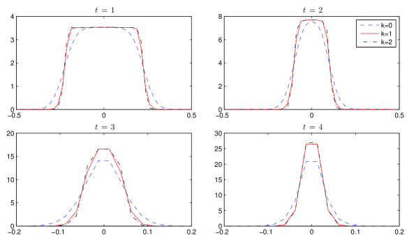
Figure 4.2. $F(t,v)$ at time $t=1,2,3,4$ for DG schemes.

4.3. Clusters vesus flocking

It is known that flocking is not ganranteed if the influence function is compactly supported, especially when (2.3) does not hold. Multiple clusters might form as time goes. This example is designed to compare the two asymptotic behaiviors. In fact, our DG scheme captures both flocking and clusters very well. Let

$$f_{0}(x,v)=\chi_{-.5<x<-.4}\cdot\chi_{.4<v<.5}+\chi_{.4<x<.5}\cdot\chi_{-.5<v<-.4}.$$

It represents two groups, where the left group is travelling to the right and the right group is travelling to the left. We consider two different influence functions:

$$\phi_{1}(r)=\chi_{r<.8},\quad\phi_{2}(r)=\chi_{r<.4}.$$

Both functions are compactly supported. Yet $\phi_{1}$ is much stronger than $\phi_{2}$. In particular, $\phi_{1}(r)\geq\phi_{2}(r)$.

Figure 4.3 shows the evolution of the CS model under two influence functions. We observe that with strong influence $\phi_{1}$, the system converges to a flock. In contrast, with relatively weak influence $\phi_{2}$, the interaction is not strong enough and multiple clusters are forming in large time.

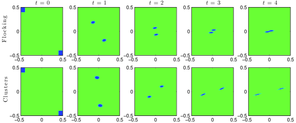
Figure 4.3. Flocking vesus cluster formation.

4.4. Cucker-Smale vesus Motsch-Tadmor

We end this paper with a nice example to compare CS and MT setups numerically.

Motsch and Tadmor in [11] discuss a drawback for CS model which motivates their model. In the particle CS model, “the motion of an agent is modified by the total number of agents even if its dynamics is only influenced by essentially a few nearby agents.” For initial configuration far from equilibrium, CS model has poor performance in modeling the dynamics. The MT setup overcomes the drawback by normalizing the influence not by the total number of agents (or total mass), but by the total influence of each agent.

The following example is design to compare the results of the two setups with an initial configuration far from equilibrium. Our DG schemes have good performances on both setups. It captures the difference of the two models in kinetic level, which agrees with the discussion in [11].

Consider the initial configuration as a combination of a small group (with mass .02) and a large flock (with mass .98) far away

$$f_{0}(x,v)=\chi_{|x|<.1}\chi_{|v|<.05}+.98\delta(x-5)\delta(v-1),$$

with compactly supported influence function $\phi(r)=(1-r)^{2}\chi_{r<1}$. It is easy to see that the large flock never interact with the small group.

Figure 4.4 shows numerical results of the evolutions of the small group in both CS and MT setups. We observe that under CS setup, the faraway large flock eliminates the interactions inside the small group. The evolution is almost like a pure transform. In contrast, MT setup yields the reasonable flocking behavior for the small group.

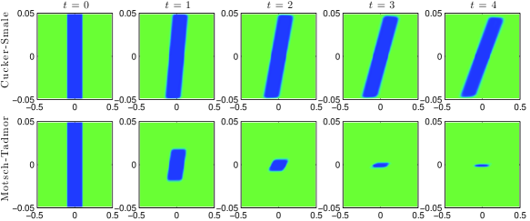
Figure 4.4. Evolution of the small group under 2 models.

References

• [1] A. L. Bertozzi, J. A. Carrillo and T. Laurent, Blow-up in multidimensional aggregation equations with mildly singular interaction kernels, Nonlinearity 22, no. 3, (2009): 683–710.
• [2] J. A. Carrillo, M. Fornasier, J. Rosado and G. Toscani, Asymptotic flocking dynamics for the kinetic Cucker-Smale model, SIAM Journal on Mathematical Analysis, 42, no. 1, (2010): 218–236.
• [3] G.-Q. Chen and H. Liu, Formation of $\delta$-shocks and vacuum states in the vanishing pressure limit of solutions to the Euler equations for isentropic fluids, SIAM journal on mathematical analysis 34, no. 4, (2003): 925–938.
• [4] B. Cockburn and C.-W. Shu, TVB Runge-Kutta Local projection discontinuous Galerkin finite element method for conservation law II: General framework, Mathematics of Computation, 52, (1989): 411–435.
• [5] F. Cucker and S. Smale, Emergent behavior in flocks, IEEE Trans. Autom. Control, 52, no. 5, (2007): 852–862.
• [6] G. Dimarco and L. Pareschi, Numerical methods for kinetic equations, Acta Numerica, 23 (2014): 369–520.
• [7] S. Gottlieb, C.-W. Shu and E. Tadmor, Strong stability preserving high-order time discretization methods, SIAM Review, 43, (2001): 89–112.
• [8] S.-Y. Ha and J.-G. Liu, A simple proof of the Cucker-Smale flocking dynamics and mean-field limit, Commun. Math. Sci., 7, no. 2, (2009): 297–325.
• [9] S.-Y. Ha and E. Tadmor, From particle to kinetic and hydrodynamic descriptions of flocking, Kinetic and Related Models, 1, no. 3, (2008): 415–435.
• [10] R. McLachlan and G. Quispel, Splitting methods, Acta Numerica 11.0 (2002): 341-434.
• [11] S. Motsch and E. Tadmor, A new model for self-organized dynamics and its flocking behavior, J. Stat. Phys, 144(5) (2011) 923–947.
• [12] W.H. Reed and T.R. Hill, Triangular mesh methods for the Neutron transport equation, Los Alamos Scientific Laboratory Report LA-UR-73-479, Los Alamos, NM, 1973.
• [13] C.-W. Shu, Essentially non-oscillatory and weighted essentially non-oscillatory schemes for hyperbolic conservation laws, Springer Berlin Heidelberg, 1998.
• [14] E. Tadmor and C. Tan, Critical thresholds in flocking hydrodynamics with nonlocal alignment, to appear at Phil. Trans. R. Soc. A.
• [15] Y. Yang and C.-W. Shu, Discontinuous Galerkin method for hyperbolic equations involving $\delta$-singularities: negative-order norm error estimates and applications, Numerische Mathematik, (2013): 1–29.
• [16] Y. Yang, D. Wei and C.-W. Shu, Discontinuous Galerkin method for Krause‘¯s consensus models and pressureless Euler equations, Journal of Computational Physics, 252, (2013): 109–127.
• [17] X. Zhang and C.-W. Shu, Maximum-principle-satisfying and positivity-preserving high order schemes for conservation laws: Survey and new developments, Proceedings of the Royal Society A, 467, (2011): 2752–2776.
• [18] X. Zhang and C.-W. Shu, A minimum entropy principle of high order schemes for gas dynamics equations, Numerische Mathematik, 121, (2012): 545–-563.