*

TREE ORIENTED DATA ANALYSIS

Sean Skwerer

A dissertation submitted to the faculty at the University of North Carolina at Chapel Hill in partial fulfillment of the requirements for the degree of Doctor of Philosophy in the Department of Statistics and Operations Research.

Chapel Hill

2014

Approved by:

Scott Provan

J.S. Marron

Ezra Miller

Gabor Pataki

Shu Lu

Complex data objects arise in many areas of modern science including evolutionary biology, nueroscience, dynamics of gene expression and medical imaging. Object oriented data analysis (OODA) is the statistical analysis of datasets of complex objects. Data analysis of tree data objects is an exciting research area with interesting questions and challenging problems. This thesis focuses on tree oriented statistical methodologies, and algorithms for solving related mathematical optimization problems.

This research is motivated by the goal of analyzing a data set of images of human brain arteries. The approach we take here is to use a novel representation of brain artery systems as points in phylogenetic treespace. The treespace property of unique global geodesics leads to a notion of geometric center called a Fréchet mean. For a sample of data points, the Fréchet function is the sum of squared distances from a point to the data points, and the Fréchet mean is the minimizer of the Fréchet function.

In this thesis we use properties of the Fréchet function to develop an algorithmic system for computing Fréchet means. Properties of the Fréchet function are also used to show a sticky law of large numbers which describes a surprising stability of the topological tree structure of sample Fréchet means at that of the population Fréchet mean. We also introduce non-parametric regression of brain artery tree structure as a response variable to age based on weighted Fréchet means.

For Robert and Laurie, my beloved and caring parents.

PREFACE

This thesis is based on collaborative work with my advisors J. S. Marron and Scott Provan in the domain of tree oriented data analysis. Chapter 1, which provides an overview of tree oriented data analysis and background material, is the original work of the student.

Chapter 2, which describes the treespace Fréchet mean optimization problem, and related theory and methods, is the original work of the student. Section 2.1 provides an overview and discussion of the problem, and these perspectives are an original contribution by the student. Section 2.2 and section 2.3 focus on summarizing existing theory and methodology. Sections 2.4 and 2.5 contain novel unpublished research by the student.

Chapter 3 summarizes data analytic results. This analysis was conducted by the student, with one exception, the result attributed to Megan Owen in Section 3.1. The discussion of Fréchet mean degeneracy in this chapter is an extension of research from a paper written by this student in collaboration with a number of authors (see reference) Skwerer et al., (2014).

Chapter 4 contains novel theoretical analysis by the student. Section 4.1 contains background material. Section 4.2 provides a summary of related research that the student contributed to as part of a collaborative research group. Section 4.3 contains an original presentation of basic definitions and novel unpublished results by the student. Section 4.4 contains the main result of the chapter which is unpublished research by the student.

Chapter 5 contains a novel method for regression of tree data objects against a Euclidean response variable. This method was described by J. S. Marron and implemented by the student. The data analysis was conducted by the student. This is unpublished research.

0.5em 0.5em

1em 2em

1.0in

LIST OF ABBREVIATIONS AND SYMBOLS

BHV	Billera, Holmes, and Vogtman
LLN	Law of Large Numbers
OODA	Object Oriented Data Analysis
SLLN	Strong Law of Large Numbers

CHAPTER 1: INTRODUCTION

1.1   Dissertation Overview

Complex data objects arise in many areas of modern science including evolutionary biology, longitudinal studies, dynamics of gene expression and medical imaging. Object oriented data analysis (OODA) is the statistical analysis of datasets of complex objects. The atoms of a statistical analysis are traditionally a number or a vector of numbers. In functional data analysis the atoms of interest are curves; for excellent treatment of functional data analysis see Ramsay and Silverman, (2002, 2005). OODA progresses from functions to more complex objects such as images, two-dimensional or three-dimensional shapes, and combinatorial structures such as graphs or trees.

Data analysis of tree data objects, or tree oriented data analysis, is an exciting research area with interesting questions and challenging problems. This thesis focuses on tree oriented statistical methodologies, and algorithms for solving related mathematical optimization problems. The mathematical focus of this thesis is driven by the goal of analyzing a data set of images of human brain arteries collected by the CASILab at UNC-CH Bullitt et al., (2008). From this perspective, this thesis is aimed at making contributions to morphology, the study of the form and structure of organisms.

In this thesis, trees are primarily modeled as points in Billera, Holmes, Vogtman treespaces. The original motivation for creating BHV treespaces was to create a firm mathematical basis for statistical inference of evolutionary histories by developing a geometric space of phylogenetic trees. In phylogenetics, trees can be used as abstract representations of evolutionary histories. In such an abstraction the root represents some common ancestor, the leaves represent species, branches represent speciation events, and length represents passage of time. A phylogenetic tree, (i) is a tree, (ii) has a positive length associated with each of its edges, and (iii) has leaves which are in bijection with an index set $\{0,1,\ldots,r\}$, which corresponds to a list of species. A BHV treespace is a geometric space of all phylogenetic trees with leaves in bijection with the same index set i.e. $\{0,1,\ldots,r\}$. For a more detailed description of phylogenetic trees and BHV treespaces see Sec. 1.2.

A central question of tree oriented data analysis is “what are appropriate notions of mean and variance for a set of trees?” Typically, the mean of a dataset is specified as the sum of the observations divided by the number of observations. The mean of real numbers could also be specified as the solution to an optimization problem. An arithmetic mean is the real number that minimizes the sum of squared distances to data points. A more general notion of mean for metric spaces, called a Fréchet mean (a.k.a, barycenter or center of mass), is a point that minimizes the sum of squared distances to the data points. The Fréchet mean is equivalent to the arithmetic mean in the case when data points are vectors. BHV treespaces have nice properties for statistics, including the existence of a unique shortest path between every pair of points, and the existence of a unique Fréchet mean for a set of points. The focus of Ch. 2 is mathematical theory and methods for solving Fréchet mean optimization problems defined for data sets on BHV treespace.

Prior to the research for this thesis, tube tracking algorithms were applied to a brain angiography dataset from the CASILab to reconstruct 3D models for the brain artery systems i.e. tubular 3D trees Aylward and Bullitt, (2002). The main research advance for representing these trees as points in a BHV treespace was finding a morphologically interpretable fixed index set. The index set used in this research was determined by a technology in neuroimage analysis, called group-wise landmark based shape correspondence, which optimally places landmarks on the cortical surface of each member in a sample. This algorithm simultaneously optimizes a term which spreads landmarks out in each subject and a term which forces landmarks to similar positions for all subjects. More details about this representation of artery trees as points in a BHV treespace are explained in Sec. 1.3.

Results from analysis of this cortical landmark and brain artery data using Fréchet means in BHV treespaces are presented in Ch. 3. In summary, these results show there is little similarity in the topological connections of brain arteries from the base of the brain to points where arteries are nearest to cortical landmarks, with the level of resolution available.

Fréchet means in BHV treespaces exhibit an unusual stability property which is known as stickiness. Contrasting the typical behavior of sample means, where typically small changes in the data result in small changes in the sample mean, stickiness refers to the phenomenon of the sample mean sticking in place regardless of small changes in the dataset. Stickiness examples and a rigorous definition for stickiness are presented in Ch. 4. The observation of this property was attributed to Seth Sullivant, and studied further by the the SAMSI working group for data sample on manifold stratified spaces, e.g. data sampled from BHV treespaces, during the 2012 Object Oriented Data Analysis program at SAMSI. In this thesis, a new contribution to stickiness research is made, we characterize the limiting behavior of Fréchet sample means on BHV treespaces as obeying a sticky law of large numbers. This is the main result in Ch. 4.

Kernel smoothing is a flexible method for studying the relationships between variables. It is used in estimating probability densities and in regression. In Ch. 5, we present a novel method for kernel smoothing regression of tree-valued response against a real-valued predictive variable. This method is applied to the brain artery systems from the CASILab which will first be introducted in Sec. 1.3.

The rest of this chapter is about phylogenetic trees and mapping brain artery trees to phylogenetic treespace.

1.2   Phylogenetic trees and BHV treespaces

1.2.1   Graphs and trees

A graph is a set of points, called vertices (use vertex for a single point), and a set of lines connecting pairs of vertices, called edges. A tree is a connected graph which has no cycles of edges and vertices. The degree of a vertex is the number of edges connected to it. The vertices of a tree with degree one are called leaves, and the edges connected to them are called pendants. Non-leaf vertices are called interior vertices. Edges which are not connected to leaves are called interior edges. An edge weighted tree is a tree $T$ together with a positive length $|e|_{T}$ associated with every edge $e\in T$. Contracting an edge means its length shrinks to zero thereby identifying its two endpoints to form a single vertex. A tree topology $T^{\prime}$ that is created by contracting some edges in a tree $T$ is called a contraction of $T$. A star tree is a tree with only pendant edges.

1.2.2   Phylogenetic trees

Evolutionary histories or hierarchical relationships are often represented graphically as phylogenetic trees. In biology, the evolutionary history of species or operational taxonomic units (OTU’s) is represented by a tree. Figure 1.1 is a very early graphical depiction of a phylogenetic tree from Haeckel, (1866).

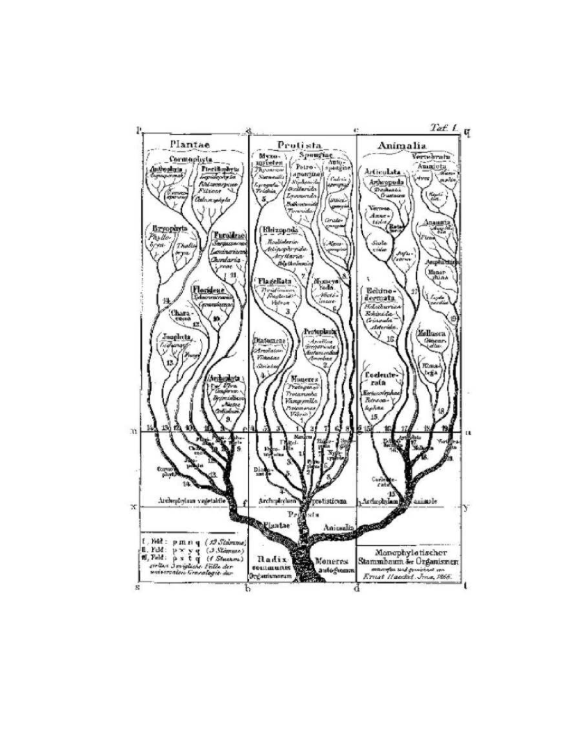
Figure 1.1: Phylogenetic tree depicting divergence of plants, protozoa, and animal kingdoms, Haeckel (1866).

The root of the tree corresponds to a common ancestor. Branches indicate speciation of a nearest common ancestor into two or more distinct taxa. The leaves of the tree correspond to the present species whose history is depicted by the tree.

A labeled tree is a tree $T$ with $r+1$ leaves distinctly labeled using the index set $I=\{0,1,\ldots,r\}$. A phylogenetic tree is a labeled edge-weighted tree. The set of edges for a tree $T$ is written $E_{T}$. Edge $e$ in $T$ is associated with a split, $X_{e}\cup\bar{X}_{e}$ in $T$. This is a partition of $I$ into two disjoint sets of labels, $X_{e}$ and $\bar{X}_{e}$ on the two components of $T$ that result from deleting $e$ from $T$, with $X_{e}$ containing the index $0$. The topology of a phylogenetic tree is the underlying graph and pendant labels separated from the edge lengths. The topology of a phylogenetic tree is uniquely represented by the set of splits associated with its edges. Formally, two splits $X_{e}\cup\bar{X}_{e}$ and $X_{f}\cup\bar{X}_{f}$ are compatible if and only if $X_{e}\subset X_{f}$ and $\bar{X}_{f}\subset\bar{X}_{e}$, or $X_{f}\subset X_{e}$ and $\bar{X}_{e}\subset\bar{X}_{f}$. Compatibility can be interpreted in terms of subtrees: the subtree with leaves in bijection with $\bar{X}_{e}$ contains the subtree with leaves in bijection with $\bar{X}_{f}$, or vice versa. If every pair of splits in a set of splits is compatible then that set is said to be a compatible set. Each distinct set of compatible splits is equivalent to a unique phylogenetic tree topology. A maximal tree topology is one in which no additional interior edges can be introduced i.e. $|E_{T}|=2r-1$, or equivalently every interior vertex has degree 3.

1.2.3   Construction of BHV Treespaces

A BHV treespace, $\mathcal{T}_{r}$ is a geometric space in which each point represents a phylogenetic tree having leaves in bijection with a fixed label set $\{0,1,2,\ldots,r\}$.

A non-negative orthant is a copy of the subset of $n$-dimensional Euclidean space defined by making each coordinate non-negative, $\mathbb{R}^{n}_{\geq 0}$. Here, only non-negative orthants are used, so we use orthant to mean non-negative orthant. An open orthant is the set of positive points in an orthant. Phylogenetic treespace is a union of many orthants, each corresponding to a distinct tree topology, wherein the coordinates of a point are interpreted as the lengths of edges. For a given set of compatible edges $E$, the associated orthant is denoted $\mathcal{O}(E)$, and for a given tree $T$, the orthant in treespace containing that point is denoted $\mathcal{O}(T)$. Trees in $\mathcal{T}_{r}$ have at most $r-2$ interior edges. Each orthant of dimension $r-2$ corresponds to a combination of $r-2$ compatible edges. Orthants are glued together along common faces. The shared faces of facets with $k$ positive coordinates are called the $k$-dimensional faces of treespace.

Take $\mathcal{T}_{4}$ as an example. There are fifteen possible pairs of compatible edges. Each compatible pair is associated with a copy of $\mathbb{R}^{2}_{\geq 0}$, one axis of the orthant for each edge in the pair. The fifteen orthants are glued together along common axes. Views of the two main features of $\mathcal{T}_{4}$ are displayed in Figure 1.2. See Figure 1.3 for a visualization of the split-split compatibility graph of $\mathcal{T}_{4}$ .

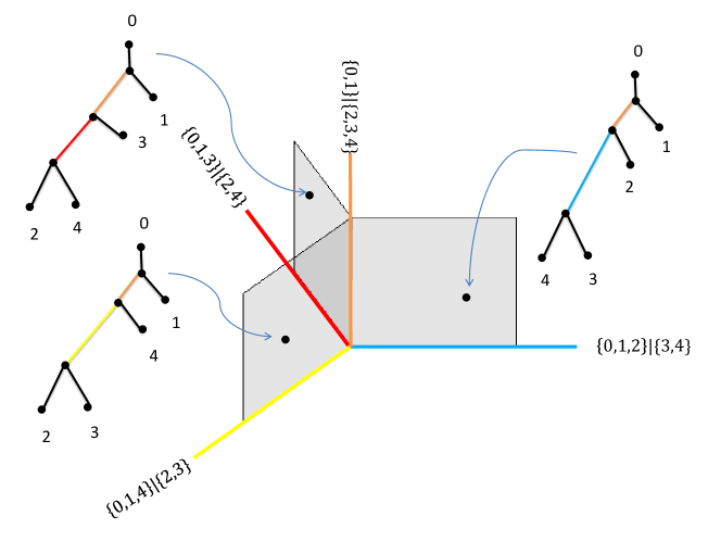
(a) An open half book with three pages. In this diagram the pages of the book are three copies of $\mathbb{R}_{\geq 0}^{2}$ and the spine is a copy of $\mathbb{R}_{\geq 0}$. The spine is labeled with the split $\{0,1\}|\{2,3,4\}$. Each page has the spine as one axis and the other axis is labeled with a split compatible with $\{0,1\}|\{2,3,4\}$. In $\mathcal{T}_{4}$ every one of the ten splits of $\{0,1,2,3,4\}$ is the label for the spine of the open half book.

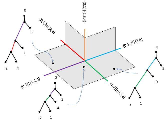
(b) A five-cycle. A five-cycle is five copies of $\mathbb{R}^{2}_{\geq 0}$ glued together along commonly labeled axes and at their origins.

Figure 1.2: Spaces called a half-open book with three pages, depicted in (a) and a five cycle of quadrants, depicted in (b), appear in $\mathcal{T}_{4}$ repeatedly. For a global view of the structure of $\mathcal{T}_{4}$ see Fig. 1.3.

Each clique in the split-split compatibility graph represents a compatible combination of splits, or equivalently the topology of a phylogenetic tree. A graph is complete if there is an edge between every pair of vertices. In a graph, a clique is a complete subgraph. Each full phylogenetic tree is a maximal clique in the split-split compatibility graph because a clique represents a set of mutually compatible splits. The split-split compatibility graph of $\mathcal{T}_{4}$ has fifteen maximal cliques, each of which is represented an edge in the graph. The split-split compatibility graph of $\mathcal{T}_{4}$ determines how the orthants of $\mathcal{T}_{4}$ are glued.

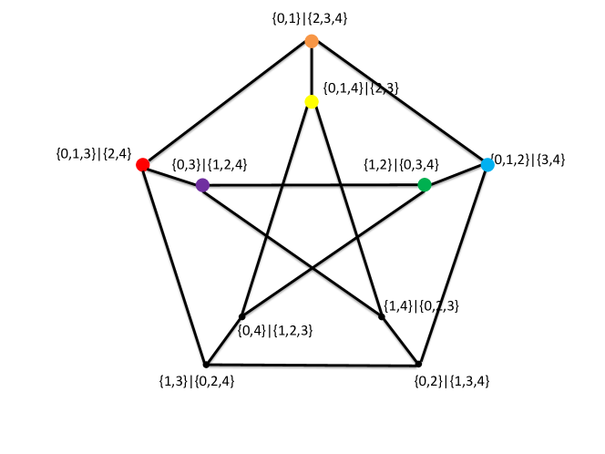
Figure 1.3: Split-split compatibility graph of ${\mathcal{T}}_{4}$. Each split has a node. Two splits are compatible if they are joined by an arc. This shows the overall connectivity of $T_{4}$, all possible splits for $\{0,1,2,3,4\}$, and all possible topologies for 4-trees. Each vertex and the three edges emanating from it in the graph corresponds to a copy of an open book like in Figure 1.2(a). Each five-cycle in the graph is a copy of a five-cycle depicted in Figure 1.2(b)

1.3   Brain artery data

The brain artery trees used in this study were reconstructed from a data set of Magenetic Resonance (MR) brain images collected by the CASILab at the University of North Carolina at Chapel Hill. This data set is publicly available and hosted at the MIDAG website Bullitt et al., (2008). The database has images for various magnetic resonance modalities, including T1, T2, Magenetic Resonance Angiography (MRA), and Diffusion Tensor Imaging (DTI). The study enrolled 109 apparently healthy subjects. Each image is tagged with subject features of age, sex, handedness and self-identified race. The MRA was aquired at 0.5 x 0.5 x 0.8 mm³ accuracy.

Arteries branch out mostly as a tree from the heart and deliver blood to the entire body. In particular arteries transport oxygen and nutrient-rich blood to the brain. Magnetic Resonance Angiography (MRA) is a technique in medical imaging to visualize arteries. MRA uses the fact that blood flowing in the arteries has a distinct magnetic signature. Full 3D image acquisition is achieved by combining cross sectional 2D images. See Figures 1.4 and 1.5 below for an MRA slice and an artery reconstruction for the same subject. A limiting factor is that MRA has a resolution threshold and consequently there are arteries that are too small for detection. MRA detects only arteries which feed blood rich with oxygen and nutrients to the body, and not veins which carry depleted blood back to the heart.

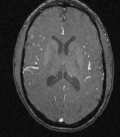
Figure 1.4: One slice of a Magnetic Resonance Angiography (MRA) image. Bright regions indicate blood flow. Bright regions are tracked through MRA slices to recover arteries tubes as shown in Figure 1.5.

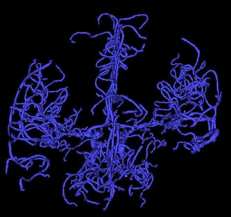
Figure 1.5: The data object is a reconstructed brain artery tree consisting of four subtrees, left, right, anterior, and posterior. The goal of this research is statistical analysis of a sample of such data objects.

The arteries visible in MRA are generally naturally described as a tree. In most regions of the body and at the level of resolution possible, arteries branch like a tree without any loops. A major part of this research has been opening up the possibility of using the space of phylogenetic trees as a mathematical basis for developing statistical methods for the study of artery trees. Phylogenetic trees have a common leaf set. However artery trees do not. A common leaf set is artificially introduced by determining points on the cortical surface that correspond across different people. The next section describes the details of representing brain artery systems as points in BHV treespace.

1.4   Mapping Brain Artery Systems to BHV treespace

Figure 1.6 gives a detailed view of artery centerlines. Each tree consists of branch segments, and each branch segment consists of a sequence of spheres fit to the bright regions in the MRA image. The sphere centers are 3D points on the center line of the artery, and the radius approximates the arterial thickness. A method for visualizing the structure of large trees was used to detect any remaining discrepancies Aydin et al., 2009b .

1.4.1   Correspondence

In addition to the brain artery trees, the data set also includes reconstructions of the cortical surface. A cortical correspondence is made by determining points on the cortical surface that correspond across different people. A group-wise shape correspondence algorithm based on spatial locations is used to place landmarks on the cortical surface Oguz et al., (2008). Each landmark is located in a corresponding spot on the cortical surface in every subject. In this study we use sixty-four landmarks for the right hemisphere and sixty-four landmarks for the left hemisphere (see Figure 1.6). The landmarks are combined with the artery tree by the following procedure. For each landmark, find the closest point on the tree of artery centerlines, called the landmark projection (see Figure 1.6). Each landmark and the line segment to its closest point become part of the tree. The tree is extracted by tracing the parts of the tree that are between the root and the landmarks. Any parts of the artery tree that are not between a landmark projection and the base are trimmed (see Figure 1.6). The base of the tree, called the root, and the 128 landmarks, add up to a total of 129 common leaves. Once the tree has been extracted each edge is associated with a positive length. The weight for each interior edge is the arc-length for the centerline of the artery tube. The pendant for each landmark has length equal to the projection distance plus the artery tube length from the projection point to the nearest artery branch. The pendant length for the root of the tree is zero.

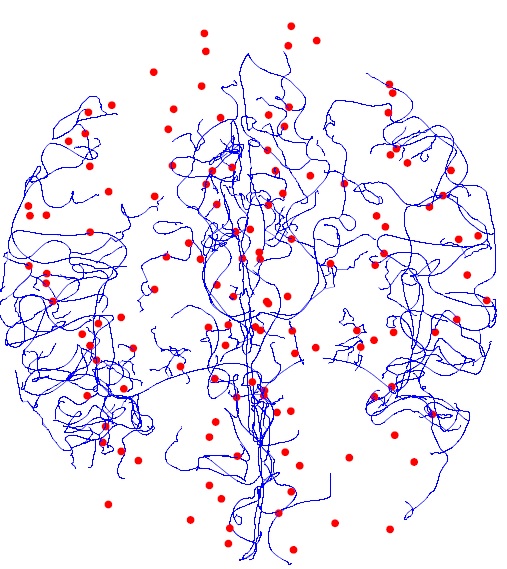
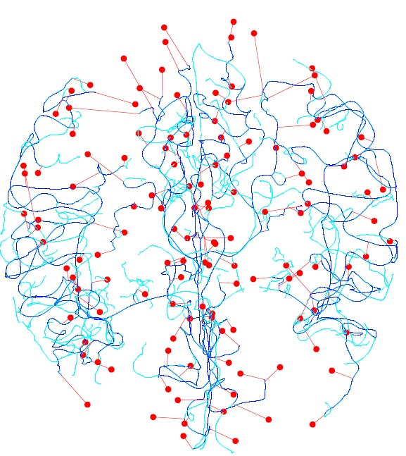
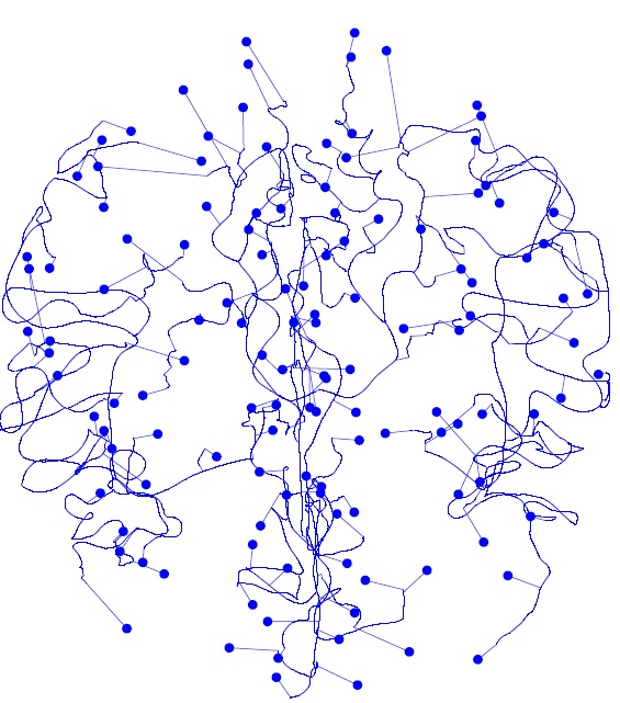
Figure 1.6: Illustrates steps for cortical correspondence. (a) Artery centerlines (blue) with the cortical landmarks (red). (b) Find the closest point on the artery tree to each landmark (red segments are landmark projections). Arteries which are not between the landmark projections and the base (cyan) are trimmed. (c) The result of this procedure is a cortical correspondence tree.

1.5   Other approaches to tree oriented data analysis

The branching structures of blood arteries and pulmonary airways are naturally modeled as trees. There is a large scope for progress in statistics for a population of trees. Currently, at the time that this dissertation is being written, research in tree oriented data analysis includes four major directions: combinatorial trees, Dyck paths, treeshapes and phylogenetic trees.

A seminal papaer in the combinatorial tree approach to studying populations of anatomical trees laid foundations by proposing a metric, several notions of center, variation, and a method of principal components Wang and Marron, (2007). Later fast PCA algorithms for combinatorial trees were developed Aydin et al., 2009a . The most recent innovation for combinatorial tree is smoothing method for nonparametric regression with combinatorial tree structures as response variables against a univariate Euclidean predictor Wang et al., (2011) .

Another approach uses a Dyck path mapping of trees to curves Harris, (1952). A Dyck path for a tree is produced by recording the distance on the tree to the root vertex during a depth first left to right traversal. Representing trees as Dyck paths opens up the possibility to use methods such as functional PCA Shen et al., (2012).

The treeshape approach is an area of active research. A tree-shape is a graph theoretic tree with a real matrix of fixed dimensions associated with each edge of the tree. Tree-shapes and statistics for tree-shapes were introduced in Feragen et al., (2012). This approach allows very general descriptions of trees and thus allows for much richer representations of anatomical trees such as lungs or arteries than the above approaches. The generality of this approach comes with the cost of a very complicated sample space. A related approach, unlabled-trees, is a special case of treeshape, where the edge attributes are restricted to be non-negative numbers.

1.5.1   BHV treespace geodesics

We now give an explicit description of geodesics in treespace.

Let $X\in\mathcal{T}_{r}$ be a variable point and let $T\in\mathcal{T}_{r}$ be a fixed point. Let $\Gamma_{XT}=\{\gamma(\lambda)|0\leq\lambda\leq 1\}$ be the geodesic path from $X$ to $T$. Let $C$ be the set of edges which are compatible in both trees, that is the union of the largest subset of $E_{X}$ which is compatible with every edge in $T$ and the largest subset of $E_{T}$ which is compatible with every edge in $X$.

The following notation for the Euclidean norm of the lengths of a set of edges $A$ in a tree $T$ will be used frequently,

$$||A||_{T}=\sqrt{\sum_{e\in A}{|e|_{T}^{2}}}$$ (1.1)

or without the subscript when it is clear to which tree the lengths are from.

A support sequence is a pair of disjoint partitions, $A_{1}\cup\ldots\cup A_{k}=E_{X}\setminus C$ and $B_{1}\cup\ldots\cup B_{k}=E_{T}\setminus C$.

Theorem 1.5.1.

Owen and Provan, (2009) A support sequence $(\mathcal{A},\mathcal{B})=(A_{1},B_{1}),\ldots,(A_{k},B_{k})$ corresponds to a geodesic if and only if it satisfies the following three properties:

• For each $i>j$, $A_{i}$ and $B_{j}$ are compatible

• $\frac{\lVert A_{1}\rVert}{\lVert B_{1}\rVert}\leq\frac{\lVert A_{2}\rVert}{\lVert B_{2}\rVert}\leq\ldots\leq\frac{\lVert A_{k}\rVert}{\lVert B_{k}\rVert}$

• For each support pair $(A_{i},B_{i})$, there is no nontrivial partition $C_{1}\cup C_{2}$ of $A_{i}$, and partition $D_{1}\cup D_{2}$ of $B_{i}$, such that $C_{2}$ is compatible with $D_{1}$ and $\frac{\lVert C_{1}\rVert}{\lVert D_{1}\rVert}<\frac{\lVert C_{2}\rVert}{\lVert D_{2}\rVert}$

The geodesic between $X$ and $T$ can be represented in ${\mathcal{T}}_{n}$ with legs

$$\Gamma_{l}=\left\{\begin{array}[]{ll}\left[\gamma(\lambda):\;\frac{\lambda}{1-\lambda}\leq\frac{\lVert A_{1}\rVert}{\lVert B_{1}\rVert}\right],&l=0\\[6.99997pt] \left[\gamma(\lambda):\;\frac{\lVert A_{i}\rVert}{\lVert B_{i}\rVert}\leq\frac{\lambda}{1-\lambda}\leq\frac{\lVert A_{i+1}\rVert}{\lVert B_{i+1}\rVert}\right],&l=1,\ldots,k-1,\\[6.99997pt] \left[\gamma(\lambda):\;\frac{\lambda}{1-\lambda}\geq\frac{\lVert A_{k}\rVert}{\lVert B_{k}\rVert}\right],&l=k\end{array}\right.$$

The points on each leg $\Gamma_{l}$ are associated with tree $T_{l}$ having edge set

$$\begin{array}[]{rcl}E_{l}&=&B_{1}\cup\ldots\cup B_{l}\cup A_{l+1}\cup\ldots\cup A_{k}\cup C\end{array}$$

Lengths of edges in $\gamma(\lambda)$ are

$$|e|_{\gamma(\lambda)}=\displaystyle\left\{\begin{array}[]{ll}\frac{(1-\lambda)\lVert A_{j}\rVert-\lambda\lVert B_{j}\rVert}{\lVert A_{j}\rVert}|e|_{X}&e\in A_{j}\\[10.00002pt] \frac{\lambda\lVert B_{j}\rVert-(1-\lambda)\lVert A_{j}\rVert}{\lVert B_{j}\rVert}|e|_{T}&e\in B_{j}\\[15.00002pt] (1-\lambda)|e|_{X}+\lambda|e|_{T}&e\in C\\ \end{array}.\right.$$

The length of $\Gamma$ is

$$d(X,T)=\bigg{\Arrowvert}(\lVert A_{1}\rVert+\lVert B_{1}\rVert,\ldots,\lVert A_{k}\rVert+\lVert B_{k}\rVert,|e_{C}|_{{}_{X}}-|e_{C}|_{{}_{T}})\bigg{\Arrowvert}$$ (1.2)

and we call this the geodesic distance from $X$ to $T$.

CHAPTER 2: Methods for Fréchet Means in Phylogenetic Treespace

2.1   Introduction

The central research problem of this chapter is efficient computation of the Fréchet mean of a discrete sample of points in BHV treespaces. The novel algorithmic system designed in this research project improves upon the current solution methodologies in Miller et al., (2012) Bac̆àk, (2012). These methods are applied to the sample of brain artery trees introduced in Chapter 1.

The contents of this Chapter are organized as follows: In Sec. 2.1.1 we define the Fréchet mean in BHV treespace, and give an overview discussion of the Fréchet optimization problem. In Sec. 2.2 we present global methods for optimizing the Fréchet function i.e. methods which can move from one orthant of treespace to another. In Sec. 2.3 we describe how the combinatorics of treespace geodesics lead to polyhedral subdivision of treespace into regions where the Fréchet function has a fixed algebraic form. The focus of Sec. 2.4 is differential properties of the Fréchet function. In Sec. 2.5.1, a method finding the minimizer of the Fréchet function in a fixed orthant of treespace is presented. Application of these method to brain artery systems is the focus of Ch. 3.

2.1.1   Fréchet means in BHV treespace

For a given data set of $n$ phylogenetic trees $T^{1},T^{2},\ldots,T^{n}$ in $\mathcal{T}_{r}$, the Fréchet function is the sum of squares of geodesic distances from the data trees to a variable tree $X$. A geodesic $\gamma:[0,1]\to\mathcal{T}_{r}$ is the shortest path between its endpoints. The geodesic from $X$ to $T^{i}$ is characterized by a geodesic support, $(\mathcal{A}^{i},\mathcal{B}^{i})=\left((A^{i}_{1},B^{i}_{1}),\ldots,(A^{i}_{k^{i}},B^{i}_{k^{i}})\right)$ (Thm. 1.5.1). Given the geodesic supports $(\mathcal{A}^{1},\mathcal{B}^{1}),\ldots,(\mathcal{A}^{n},\mathcal{B}^{n})$ the Fréchet function is

$$F(X)=\sum_{i=1}^{n}d(X,T^{i})^{2}=\sum_{i=1}^{n}\left(\sum_{l=1}^{k^{i}}(\lVert x_{A_{l}^{i}}\rVert+\lVert B_{l}^{i}\rVert)^{2}+\sum_{e\in C^{i}}(|e|_{T}-|e|_{T^{i}})^{2}\right).$$ (2.1)

The objective is to solve the Fréchet optimization problem

$$\min_{X\in\mathcal{T}_{r}}{F(X)}$$ (2.2)

Elementary Fréchet function properties:

• The Fréchet function is continuous because the geodesic distances $d(X,T^{i})$ are continuous Owen and Provan, (2009); Miller et al., (2012).

• The Fréchet function $F(X)$ is strictly convex Sturm, (2003), that is $F\circ\gamma:[0,1]\to\mathbb{R}$ is (strictly) convex for every geodesic $\gamma(\lambda)$ in $\mathcal{T}_{r}$.

As a consequence of these properties we have the following result.

Lemma 2.1.1.

The Fréchet mean exists and is unique.

Proof.

A strictly convex function either has a unique minimizer or can be made arbitrarily low. Assuming that the data points are finite, then a minimizer of the Fréchet function must also be finite. Therefore the Fréchet function has a unique minimizer. ∎

The Fréchet mean $\bar{T}$ is the unique minimizer of the Fréchet function.

2.1.1.1 Problem Discussion

The Fréchet optimization problem, in BHV treespace, requires both selecting the minimizing tree topology and specifying its edge lengths. Tree topologies are discrete and so the problem of selecting the minimizing tree topology is a combinatorial optimization problem; however it is possible to make search strategies which take advantage of the continuity of BHV treespace to find the correct tree topology. It is natural to consider this problem in two modes of search: global, i.e. strategies which change the topology and edge lengths; and local, i.e. strategies which only adjust edge lengths. One motivation to consider global search and local search separately is that the local optimization problem is convex optimization constrained to a Euclidean orthant.

The global search problem is challenging because the geometry of treespace creates difficulty in two essential parts of optimization (1) making progress towards optimality and (2) verifying optimality. In treespace a metrically small neighborhood can actually be quite large in a certain sense. In constructing the space, the topological identification of the shared faces of orthants may create points in the closure of many orthants. In terms of trees, the neighborhood around a tree $X$, $N(X)$, is comprised not only of trees with the same topology as $X$ but also trees which have $X$ as a contraction. However, the list of tree topologies which have a particular tree $X$ as a contraction can be quite large. For example, if $X$ is a star tree then $X$ is a contraction of any tree i.e. $X$ is a contraction of $(2r-3)!!$ maximal phylogenetic tree topologies.

Local optimality conditions for non-differentiable functions are based on the rate of change of the objective function along directions issuing from a point. Since the neighborhood of a point $X$ contains all trees which have $X$ as a contraction, verifying that $X$ is optimal requires demonstrating that any tree which contains $X$ as a contraction has a larger Fréchet function value. For example, when $X$ is a star tree, $N(X)$ contains every tree with the same pendants as $X$, and having infinitesimal interior edge lengths. In this sense finding a descent direction can be essentially as hard as finding the topology of the Fréchet mean itself.

Proximal point algorithms, a broad class of algorithms, are globally convergent not only for the Fréchet optimization problem, but are globally convergent for any well defined lower-semicontinuous convex optimization problem on a non-positively curved metric space Bac̆àk, (2012). This class of algorithms has nice theoretical properties, and certain implementations of proximal point algorithms are practical for the Fréchet optimization problem on non-positively curved orthant spaces.

Proximal point algorithms are applicable to optimization problems on metric spaces. The general problem is minimizing a function $f$ on a metric space $M$ with distance function $d:M\times M\to\mathbb{R}$. A proximal point algorithm solves a sequence of penalized optimization problems of the form

$$\displaystyle P_{k}(f):\min_{x^{k}}{\quad f(x^{k})+\alpha_{k}d^{2}(x^{k-1},x^{k})}$$ (2.3)

where $\alpha_{k}$ influences the proximity of a solution to the point $x^{k-1}$. Some good references for proximal point algorithms are Bačák, (2012); Bertsekas, (2011); Li et al., (2009); Rockafellar, (1976).

Implementing a generic proximal point algorithm to minimize the Fréchet function on treespace does not seem advantageous. In particular, given a non-optimal point $X^{0}$ finding a point $X$ such that $F(X)<F(X^{0})$ is not made any easier by penalizing the objective function $F(X)+\alpha d^{2}(X^{0},X)$. Penalizing the objective function with $\alpha d(X^{0})$ does not provide any additional structure for checking the neighborhood, $N(X^{0})$, of $X^{0}$ for a descent direction.

Split proximal point algorithms avoid directly tackling the complicated problem of minimizing $F(X)$ by solving many much easier subproblems. For objective functions which can be expressed as a sum of functions, $f=f^{1}+\ldots+f^{m}$, a split proximal point algorithm alternates among penalized optimization problems for each function. Let $\{1,2,\ldots,m\}$ index the functions $f^{1},\ldots,f^{m}$. A generic split proximal point algorithm is: choose some sequence $i_{1},i_{2},\ldots$ where each term in the sequence is an element of $\{1,2,\ldots,m\}$ and sequentially solve the split proximal point optimization problem:

$$\displaystyle P_{k}(f^{i_{k}}):\min_{x^{k}}{\quad f(x^{k})+\alpha_{k}d^{2}(x^{k-1},x^{k})}$$ (2.4)

Different versions of split proximal point algorithms are based on the choice of the sequence $i_{1},i_{2},\ldots$ and the choice of the sequence $\{\alpha_{k}\}$. Naturally, a split proximal point procedure can be applied to the Fréchet optimization problem by separating the Fréchet function into a sum of squared distance functions, $F(X)=d^{2}(X,T^{1})+\ldots+d^{2}(X,T^{n})$. For the Fréchet function the split proximal point optimization problem is

$$\displaystyle P_{k}(d^{2}(X^{k},T^{i_{k}})):\min_{x^{k}}{\quad d^{2}(X^{k},T^{i_{k}})+\alpha_{k}d^{2}(X^{k-1},X^{k})}$$ (2.5)

For the Fréchet mean optimization problem on a geodesic non-positively curved space, the solution to a split proximal point optimization problem can be obtained easily in terms of geodesics. The solution to $P_{k}(d^{2}(X^{k},T^{i_{k}}))$ must be on the geodesic between $X^{k-1}$ and $T^{i_{k}}$. The term $d^{2}(X^{k},T^{i_{k}})$ is the squared distance from the variable point to $T^{i_{k}}$ and the term $d^{2}(x^{k-1},x^{k})$ is the squared distance from the search point to $X^{k-1}$. Given any point, there is at least one point on the geodesic between $X^{k-1}$ and $T^{i_{k}}$ for which the value of both terms is at least as small. Since $X^{k}$ must be on this geodesic, the distance from $X^{k}$ to $X^{k-1}$ and the distance form $X^{k}$ to $T^{i_{k}}$ can be parameterized in terms of the proportion $t:0\leq t\leq 1$ along the geodesic from $X^{k-1}$ to $T^{i_{k}}$: $d(X^{k},T^{i_{k}})=(1-t)d(X^{k-1},T^{i_{k}})$ and $d(X^{k},X^{k-1})=td(X^{k-1},T^{i_{k}})$. Parameterizing $d^{2}(X^{k},T^{i_{k}})+\alpha_{k}d^{2}(X^{k-1},X^{k})$ in terms of $t$ makes $P_{k}(d^{2}(X^{k},T^{i_{k}}))$ into a problem of minimizing a quadratic function in $t$. The optimal step length is $t=\min\{1,\frac{\alpha}{1+\alpha}\}$. Even more importantly, several versions of split proximal point algorithms have been shown to converge globally to the Fréchet mean Bac̆àk, (2012). Split proximal point algorithms for Fréchet means on non-positively curved orthant spaces are discussed further in Section 2.2.

The overall strategy for minimizing the Fréchet function will be to use a split proximal point algorithm for global search and switch to a local search procedure. The motivation for switching to a local search procedure is that the if local search is initialized close to the optimal solution then faster convergence can be achieved. The local optimization problem is minimizing the Fréchet function in a fixed orthant $\mathcal{O}$. One feature of the local optimization problem is that the Fréchet function is a piecewise $C^{\infty}$ function whose algebraic form depends on the geodesic distance from $X$ to the data trees. But, the Fréchet function is only $C^{1}$ when $X$ is restricted to the interior of a maximal dimension orthant. Analysis of differential properties of the Fréchet function is presented in Sec. 2.4.

In $\mathcal{T}_{r}$, the Owen-Provan algorithm for the geodesic $\Gamma(X,T^{i})$ has complexity $O(r^{4})$, and with $n$ data points the total complexity of finding the algebraic form of $F(X)$ would be $O(nr^{4})$. New algorithms for dynamically updating the algebraic form of $F(X)$ as $X$ varies are presented in Section 2.6. Such algorithms will be especially useful in updating the objective function after small changes are made in the edge lengths of $X$; in particular these methods help accelerate local search algorithms.

Here is a high-level outline of the algorithmic system for solving the Fréchet mean optimization problem developed in this chapter:

Treespace Fréchet mean algorithm
input: $T^{1},T^{2},\ldots,T^{n},X^{0}\in\mathcal{T}_{r}$, $\epsilon>0$, $\delta>0$, $a>0$, $0<c<1$, $\{\alpha_{k}\}$, $K\in\mathbb{N}$

$F_{0}=\inf$; $F_{1}=F(X^{0})$

while $F_{1}-F_{0}>a$

SPPA for $K$ steps (Sec. 2.2)

c=1;

while $c\leq K$

$X^{k}=argmin_{X}\left\{d^{2}(X,T^{i_{k}})+\alpha_{k}d^{2}(X^{k-1},X)\right\}$

endwhile
         while approximate optimality conditions (2.5) are not satisfied

compute a descent direction $P$ (Sec. 2.5.1.1)

find a step-length, $\alpha$, satisfying decrease condition (Sec. 2.5.1.2)

let $X^{k+1}=X^{k}+\alpha P$

if $|e|<\epsilon$ then remove $e$

endwhile
endwhile

The following sections discuss implementation details and present theoretical analysis pertaining to certain aspects of the problem. The next section presents specific global search procedures, both of which are versions of split proximal point algorithms. The remaining sections focus on aspects of the local search problem.

2.2   Global search methods

Proximal point algorithms as applied to the Fréchet optimization problem have been studied in Bac̆àk, (2012) and Sturm, (2003). The former views the Fréchet mean problem from the paradigm of convex optimization while the later studies Fréchet means in the context of stochastic analysis in metric spaces of non-positive curvature. In this Chapter two global search algorithms are discussed, the Inductive Mean Algorithm, which is stochastic, and the Cyclic Split Proximal Point Algorithm, which is deterministic. Both of these are versions of split proximal point algorithms.

2.2.1   Inductive means

The Inductive Mean Algorithm is a method for calculating the Fréchet Mean based on (Sturm,, 2003, Thm. 4.7). This algorithm was developed independently in Bac̆àk, (2012) and Miller et al., (2012) and has been called Sturm’s algorithm, named after the K. T. Sturm who is attributed with its discovery in proving that inductive means converge to the Fréchet mean in the more general context of probability distributions on non-positively curved metric spaces.

Consider a sequence $(Y_{i})_{i\in\mathbb{N}}$ of independent identically distributed random observations from the uniform distribution on $\{T^{1},T^{2},\ldots,T^{n}\}$. Define a new sequence of points $(S_{k})_{k\in\mathbb{N}}$ in $\mathcal{T}_{r}$ by induction on $k$ as follows:

$$S_{1}:=Y_{1},$$

and

$$S_{k}:=\left(1-\frac{1}{k}\right)S_{k-1}+\frac{1}{k}Y_{k},$$

where the right hand side denotes the point $\frac{1}{k}$ fraction of the distance along the geodesic from $S_{k-1}$ to $Y_{k}$. The point $S_{k}$ is called the inductive mean value of $Y_{1},\ldots,Y_{k}$. The expected squared distance between $S_{k}$ and $\bar{T}$ is less than or equal to $F(\bar{T})/k$.

2.2.2   Cyclic Split Proximal Point Algorithm

Choose a permutation, $(p_{0},p_{1},\ldots,p_{n-1})$, of $\{1,2,\ldots,n\}$. Define a new sequence of points $(R_{k})_{k\in\mathbb{N}}$ in $\mathcal{T}_{r}$ by induction on $k$ as follows:

$$R_{1}:=Y_{p_{1}},$$

and

$$R_{k}:=\left(1-\frac{1}{k}\right)R_{k-1}+\frac{1}{k}Y_{p_{\left(k\operatorname{mod}n\right)}}.$$

The sequence $\{R_{k}\}$ converges to $\bar{T}$ as $k$ approaches infinity Bac̆àk, (2012).

2.3   Vistal cells and squared treespace

The value of the Fréchet function at $X$ depends on the geodesics from $X$ to each of the data trees. The goal in this section is to describe how treespace can be subdivided into regions where the combinatorial form of geodesics from $X$ to the data trees are all fixed. Descriptions of such regions will be used in analyzing the differential properties of the Fréchet function.

Analysis of the Fréchet function starts at the level of a geodesic from a variable tree $X$ to a fixed source tree $T$. Given a fixed tree $T$, a vistal cell is a region $\mathcal{V}$ of treespace where the form of the geodesic from any tree $X$ in $\mathcal{V}$ to $T$ is constant. The description of geodesics in Section 1.5.1 is now built upon further to study how the combinatorics of geodesic supports for $\Gamma(X,T)$ can vary as $X$ varies.

Definition 2.3.1.

(Miller et al.,, 2012, Def. 3.3) Let $T$ be a tree $\mathcal{T}_{r}$. Let $\mathcal{O}$ be a maximal orthant containing $T$. The previstal facet, ${\cal V}(T,\mathcal{O};\mathcal{A},\mathcal{B})$, is the set of variable trees, $X$ $\in\mathcal{O}$, for which the geodesic joining $X$ to $T$ has support $(\mathcal{A},\mathcal{B})$ satisfying $(P2)$ and $(P3)$ with strict inequalities.

The description of the previstal facet $\mathcal{V}(T,\mathcal{O};\mathcal{A},\mathcal{B})$ becomes linear after a simple change of variables. Let $x_{e}$ denote the coordinate in $\mathcal{T}_{r}$ indexed by edge $e$.

Definition 2.3.2.

(Miller et al.,, 2012, Def. 3.4) The squaring map $\mathcal{T}_{r}\to\mathcal{T}_{r}$ acts on $x\in T_{r}\subset\mathbb{R}^{E}_{+}$ by squaring coordinates:

$$(x_{e}|e\in E)\to(\xi_{e}|e\in E),\textrm{ where }\xi_{e}=x^{2}_{e}$$

Denote by $\mathcal{T}_{r}^{2}$ the image of this map, and let $\xi_{e}=x_{e}^{2}$ denote the coordinate indexed by $e\in E$. The image of an orthant in $\mathcal{T}_{r}$ is then the equivalent orthant in $T_{r}^{2}$, and the image of a previstal facet ${\cal V}(T,\mathcal{O};\mathcal{A},\mathcal{B})$ in $\mathcal{T}_{r}^{2}$ is a vistal facet denoted by ${\cal V}^{2}(T,\mathcal{O};\mathcal{A},\mathcal{B})$. With this change of variables, $\lVert S\rVert=\sum_{e\in S}{\xi_{e}}$.

The squaring map induces on the Fréchet function $F$ a corresponding pullback function

$$F^{2}(\xi)=F(\sqrt{\xi})\textrm{, where}(\sqrt{\xi})_{e}=\sqrt{\xi_{e}}.$$

Since the Fréchet function $F(X)$ has a unique minimizer $F^{2}(\xi)$ must also have a unique minimizer.

Proposition 2.3.3.

(Miller et al.,, 2012, Prop. 3.5) The vistal facet ${\cal V}^{2}(T,\mathcal{O};\mathcal{A},\mathcal{B})$ is a convex polyhedral cone in $\mathcal{T}_{r}^{2}$ defined by the following inequalities on $\xi\in\mathbb{R}^{r-2}$.

• $\xi\in\mathcal{O}$; that is, $\xi_{e}\geq 0$ for all $e\in E$, and $\xi_{e}=0$ for $e\notin E$, where $\mathcal{O}=\mathbb{R}^{r-2}_{\geq 0}$.

• $\lVert B_{i+1}\rVert^{2}$ $\displaystyle{\sum_{e\in A_{i}}\xi_{e}\leq\lVert B_{i}\rVert^{2}\sum_{e\in A_{i+1}}{\xi_{e}}}$ for all $i=1,\ldots,k-1$.

• $\lVert B_{i}\setminus J\rVert$ $\displaystyle{\sum_{e\in A_{i}\setminus I}\xi_{e}\geq\lVert J\rVert\sum_{e\in I}{\xi_{e}}}$ for all $i=1,\ldots,k$ and subsets $I\subset A_{i}$, $J\subset B_{i}$ such that $I\cup J$ is compatible.

Proposition 2.3.4.

(Miller et al.,, 2012, Prop. 3.6) The vistal facets are of dimension $2r-1$, have pairwise disjoint interiors, and cover $\mathcal{T}_{r}^{2}$. A point $\xi\in\mathcal{T}^{2}_{r}$ lies interior to a vistal facet $\mathcal{V}^{2}(T,\mathcal{O};\mathcal{A},\mathcal{B})$ if and only if the inequalities in (O), (P2), and (P3) are strict.

Points which are not on the interior of vistal facets are in vistal cells, the faces of vistal facets. A point $\xi$ is on a vistal facet precisely when some of the inequalities in (O), (P2) or (P3) are satisfied at equality. In such a situation, there is more than one valid support for the geodesic from $T$ to the pre-image $X$ of $\xi$.

A system of equations defining a vistal cell can be formed by combining the systems of equations from adjacent vistal facets and forcing appropriate constraints to equality. A canonical description of vistal cells is given in (Miller et al.,, 2012, Sec. 3.2.5).

Let $T^{1},\ldots,T^{n}$ be a set of points in $\mathcal{T}_{r}$. A region $\mathcal{V}$ in squared treespace where the geodesics $\Gamma_{XT^{1}},\dots,\Gamma_{XT^{n}}$ can be represented by a fixed set of supports is called a multi-vistal cell. A multi-vistal cell is an intersection of vistal facets of $T^{1},\ldots,T^{n}$. Multi-vistal cells and their pre-images in $\mathcal{T}_{r}$, pre-multi-vistal cells, are regions where the Fréchet function can be represented with a fixed algebraic form.

The systems of equations defining pre-vistal facets and pre-vistal cells are quadratic cones with cone points at the origin of treespace. In squared treespace, the vistal facets and vistal cells are polyhedral cones. Multi-vistal facets are also polyhedral cones with cones points at the origin of treespace, because they are intersections of polyhedral cones with cone points at the origin of treespace. This nice geometric structure is useful both in determining when a search point is on the boundary of a vistal cell, and thus when the objective function has multiple forms, and for dynamically updating the objective function during line searches, as described in Sec. 2.6.

2.4   Differential analysis of the Fréchet function in treespace

Analysis of how $F(X)$ changes with respect to $X$ provides useful insights for designing fast optimization algorithms. This analysis is aimed at providing summaries for how the value of $F(X)$ changes with respect to $X$. These results also play an important role in Ch. 4, which focuses on stickiness of Fréchet means in treespace.

Let $X$ and $Y$ be points in $\mathcal{T}_{r}$ such that $X$ and $Y$ share a multi-vistal facet. If this is the case, then either (i) $X$ and $Y$ have the same topology, (ii) $X$ is a contraction of $Y$ or (iii) $Y$ is a contraction of $X$. Assume that if the topologies of trees $X$ and $Y$ differ then $X$ is a contraction of $Y$, that is $\mathcal{O}(X)\subseteq\mathcal{O}(Y)$. Let $\Gamma(X,Y;\alpha)$ be the parameterized geodesic from $X$ to $Y$ with $0\leq\alpha\leq 1$.

Definition 2.4.1.

The directional derivative from $X$ to $Y$ is

$$F^{\prime}(X,Y)= \lim_{\alpha\to 0}\frac{F(\Gamma(X,Y;\alpha))-F(X)}{\alpha}$$ (2.6)

The main results of this section are summarized as follows: Cor. 2.4.3 gives the value of the directional derivative when $\mathcal{O}(X)=\mathcal{O}(Y)$ and Thm. 2.4.7 gives the value of the directional derivative when $\mathcal{O}(X)\subseteq\mathcal{O}(Y)$, when assuming $Y$ is contained on the interior of a multi-vistal facet. In Lem. 2.4.8 we show that when when $Y$ is on a multi-vistal face the value of the directional derivative can be expressed equivalently using any of the representations for the geodesics from $T^{1},\ldots,T^{n}$ to $Y$. In Lem. 2.4.9 and Lem. 2.4.11 we show that the directional derivative is continuous and convex with respect to $Y$ on $\mathcal{T}_{r}$. Thm. 2.4.17 states that the value of the directional derivative can be decomposed into a contribution from the change in $F(X)$ resulting in adjusting positive length edges in $X$, and a contribution from the change in $F(X)$ resulting in increasing the lengths of edges from zero.

When both $X$ and $Y$ are in the relative interior of the same maximal orthant of treespace, where the gradient at $X$ is well defined in $\mathcal{O}(Y)$, the directional derivative can be expressed in terms of the gradient at $X$ inside $\mathcal{O}(Y)$. However when $\mathcal{O}(X)\subsetneqq\mathcal{O}(Y)$, the gradient at $X$ might not be well defined in $\mathcal{O}(Y)$. Analysis of the directional derivative in the later situation, which is one of the main focuses of this section, is important because it facilitates concise specification of optimality conditions and an efficient algorithm for verifying that a point on a lower dimensional face of an orthant $\mathcal{O}$ is the minimizer of the Fréchet function within $\mathcal{O}$.

Theorem 2.4.2.

Miller et al., (2012)[Thm. 2.2] The gradient of $F$ is well defined on the interior of every maximal orthant $\mathcal{O}$.

Idea of proof. The Fréchet function is smooth in each multi-vistal facet, and it can be shown that the gradient function has the same value in every multi-vistal facet containing $X$ in the interior of $\mathcal{O}$. Therefore the gradient is well -defined on the interior of $\mathcal{O}$.

Corollary 2.4.3.

When $\mathcal{O}(X)=\mathcal{O}(Y)$ the value of directional derivative from $X$ to $Y$ can be expressed in terms of the gradient at $X$, and the differences in edge lengths $p_{e}=|e|_{Y}-|e|_{X}$, as

$$F^{\prime}(X,Y)=\sum_{e\in E_{X}}p_{e}\left[\nabla F(X)\right]_{e}$$ (2.7)

Proof.

Expression of a directional derivative of a smooth function in terms of its gradient is a standard technique in calculus. ∎

The gradient may not be well defined on a lower-dimensional orthant of treespace. For a point on a lower dimensional orthant of treespace, a well defined analogue to the gradient is the restricted gradient.

Definition 2.4.4.

Let $(A^{i}_{1},B^{i}_{1}),\ldots,(A^{i}_{k^{i}},B^{i}_{k^{i}})$ be a support sequence for the geodesic from $X$ to $T^{i}$. The restricted gradient is the vector of partial derivatives which correspond to points $Y$ with $\mathcal{O}(X)\subseteq\mathcal{O}(Y)$ and $Y-X$ parallel to the axes of $\mathcal{O}(X)$. If $|e|_{X}>0$ then

$$\left[\nabla F(X)\right]_{e} =\lim_{\Delta e\to 0}\frac{F(X+\Delta e)-F(X)}{\Delta e}$$ (2.8)

$$=\sum_{i=1}^{n}\left\{\begin{array}[]{ll}|e|_{X}\left(1+\frac{||B^{i}_{l}||}{||A^{i}_{l}||}\right)&\textrm{if $e\in A_{l}^{i}$}\\ \left(|e|_{X}-|e|_{T^{i}}\right)&\textrm{if $e\in C^{i}$}\\ \end{array}\right.$$ (2.11)

and if $|e|_{X}=0$ then $\left[\nabla F(X)\right]_{e}=0$.

When $X$ is on the interior of a maximal orthant of treespace then the restricted gradient is the same as the gradient. Note that in the case when $A^{i}_{l}=\{e\}$, $|e|_{X}\left(1+\frac{||B^{i}_{l}||}{||A^{i}_{l}||}\right)=|e|_{X}+\lVert B^{i}_{l}\rVert$.

Second order derivatives will be used in calculating Newton directions in Sec. 2.5.

Definition 2.4.5.

Let $X$ be a point in the interior of a multi-vistal cell relative to an orthant $\mathcal{O}$ of treespace. The restricted Hessian on $\mathcal{O}$ is the matrix of second order partial derivatives with entries having the following values:

$$\left[\nabla^{2}F(X)\right]_{ef}=2\sum_{i=1}^{r}{\left\{\begin{array}[]{ll}1+\frac{\lVert B_{l}^{i}\rVert}{\lVert A_{l}^{i}\rVert}-\frac{\lVert B^{i}_{l}\rVert}{\lVert A^{i}_{l}\rVert^{3}}x_{e}^{2}&\textrm{if $e=f$, $e\in A^{i}_{l}$, $|A^{i}_{l}|>1$}\\ 1&\textrm{if $e=f$, $e\in A^{i}_{l}$, $A^{i}_{l}=\{e\}$}\\ 1&\textrm{if $e=f$ $e\in C^{i}$}\\ -\frac{\lVert B^{i}_{l}\rVert}{\lVert A_{l}^{i}\rVert^{3}}x_{e}x_{f}&\textrm{if $e\neq f$ $e,f\in A_{l}^{i}$}\\ 0&\textrm{otherwise}\end{array}\right.}$$ (2.12)

If either $|e|_{X}=0$ or $|f|_{X}=0$ then $\left[\nabla^{2}F(X)\right]_{ef}=0$.

Theorem 2.4.6.

The value of the restricted gradient at a point $X$ can be expressed equivalently using the algebraic form of the Fréchet function from any of the multi-vistal facets containing $X$.

Proof.

The restricted gradient has the same value using any of the valid support sequences defined by vistal cells on the relative interior of $\mathcal{O}$. Here we verify that at $X$ the gradient of $d^{2}(X,T^{i})$ is the same for every valid support and signature. The gradient of $d^{2}(X,T^{i})$ for the support $(\mathcal{A},\mathcal{B})$ is given as follows. Let the variable length of edge $e$ in $X$ be written as $x_{e}$.

$$\frac{\partial d^{2}(X,T^{i})}{\partial x_{e}}=\left\{\begin{array}[]{ll}2\left(1+\frac{||B_{l}||}{||A_{l}||}\right)x_{e}&\textrm{if $e\in A^{i}_{l}$}\\ 2\left(x_{e}-|e|_{T}^{i}\right)&\textrm{if $e\in C^{i}$}\end{array}\right.$$ (2.13)

The geodesic $\Gamma$ has a unique support$(\mathcal{A},\mathcal{B})$ satisfying

$$\frac{\lVert A_{1}\rVert}{\lVert B_{1}\rVert}<\frac{\lVert A_{2}\rVert}{\lVert B_{2}\rVert}<\ldots<\frac{\lVert A_{k}\rVert}{\lVert B_{k}\rVert}.$$ (2.14)

From Miller et al., (2012), any other support $(\mathcal{A}^{\prime},\mathcal{B}^{\prime})$ for $\Gamma$ must have a signature $\mathcal{S}^{\prime}$ in $(P3)$ with some equality subsequences. Suppose that $A_{j}^{\prime}$ and $B_{j}^{\prime}$ are in some equality subsequence satisfying $(P2)$ with $B_{j}^{\prime}$ containing the edge $e$. Then for the support pair $A_{i}$ and $B_{i}$ such that $B_{i}$ contains $e$, it must hold that $\frac{\lVert A_{i}^{\prime}\rVert}{\lVert B_{i}^{\prime}\rVert}=\frac{\lVert A_{j}\rVert}{\lVert B_{j}\rVert}$. Now we can see that $\left(1+\frac{||B_{j}^{\prime}||}{||A_{j}^{\prime}||}\right)x_{e}=\left(1+\frac{||B_{i}||}{||A_{i}||}\right)x_{e}$, and that the gradient of $d^{2}(X,T^{i})$ is the same on every multi-vistal facet containing $X$ on the relative interior of $\mathcal{O}$. ∎

Now we extend the results for directional derivatives to the situation when $\mathcal{O}(X)\subset\mathcal{O}(Y)$.

Theorem 2.4.7.

Suppose that $Y$ lies in the interior of multi-vistal facet $V_{Y}$, and $X$ is some point in $V_{Y}$. Let $(A^{i}_{1},B^{i}_{1}),\ldots,(A^{i}_{n},B^{i}_{n})$ be the support pairs for the geodesic from $Y$ to $T^{i}$ and let $C^{i}$ be the set of edges in $Y$ which are common in $T^{i}$. Let $E_{X}$ be the set of edges with positive lengths in $X$. Let $P$ be the vector with components $p_{e}=|e|_{Y}-|e|_{X}$ so that $\Gamma(X,Y;\alpha)=X+\alpha P$, and let $Z_{\alpha}:=\Gamma(X,Y;\alpha)$. Then the value of directional derivative from $X$ to $Y$ is

$$F^{\prime}(X,Y)=\sum_{e\in E_{X}}p_{e}\left[\nabla F(X)\right]_{e}+2\sum_{i=1}^{n}\left(\sum_{l:\lVert A^{i}_{l}\rVert_{X}=0}\left(\lVert A^{i}_{l}\rVert_{P}\lVert B^{i}_{l}\rVert_{T}\right)-\sum_{e\in C^{i}\setminus E_{X}}p_{e}|e|_{T^{i}}\right).$$

Proof.

Let $Z$ be a point on the geodesic segment between $X$ and $Y$. The length of edge $e$ in $Z$ be $|e|_{Z}=|e|_{X}+\alpha p_{e}$. The Fréchet function is the sum of squared distances from a variable point to each of the data points $T^{1},\ldots,T^{n}$, so the directional derivative of the Fréchet function is the sum over the indexes of the data points of the directional derivatives of the square distances.

$$F^{\prime}(X,Y) =\lim_{\alpha\to 0}\frac{F(Z_{\alpha})-F(X)}{\alpha}$$ (2.15)

$$=\lim_{\alpha\to 0}\frac{\sum_{i=1}^{n}d^{2}(Z_{\alpha},T^{i})-\sum_{i=1}^{n}d^{2}(X,T^{i})}{\alpha}$$ (2.16)

$$=\sum_{i=1}^{n}\left(\lim_{\alpha\to 0}\frac{d^{2}(Z_{\alpha},T^{i})-d^{2}(X,T^{i})}{\alpha}\right)$$ (2.17)

For a set of edges $A$, let $\lVert A\rVert_{X}=\sqrt{\sum_{e\in A}|e|_{X}}$. If an edge $e$ has zero length in a tree, $X$, or is compatible with $X$ but not present then take $|e|_{X}$ to be $0$. The squared distance from $Z_{\alpha}$ to $T^{i}$ can be expressed as

$$d^{2}(Z_{\alpha},T^{i}) =\sum_{l=1}^{k^{i}}(\lVert A^{i}_{l}\rVert_{Z_{\alpha}}+\lVert B^{i}_{l}\rVert)^{2}+\sum_{e\in C^{i}}(|e|_{Z_{\alpha}}-|e|_{T^{i}})^{2}.$$ (2.18)

The squared distance has three types of terms: a term representing the contribution from common edges, terms for support pairs with $\lVert A^{i}_{l}\rVert_{X}>0$, and terms for support pairs with $\lVert A^{i}_{l}\rVert_{X}=0$. In the first two cases the gradient is well-defined, and taking the inner-product of the directional vector and the gradient will yield their contributions to the directional derivative. In the third case the gradient is undefined, and its value will be obtained by analyzing the limit directly as follows.

$$\left(\lim_{\alpha\to 0}\frac{\sum_{l=1}^{k^{i}}(\lVert A^{i}_{l}\rVert_{Z_{\alpha}}+\lVert B^{i}_{l}\rVert)^{2}-\sum_{l=1}^{k^{i}}(\lVert A^{i}_{l}\rVert_{X}+\lVert B^{i}_{l}\rVert)^{2}}{\alpha}\right).$$ (2.19)

Bringing out the sum and canceling in the numerators yields,

$$\sum_{l=1}^{k^{i}}\lim_{\alpha\to 0}\frac{\lVert A^{i}_{l}\rVert^{2}_{Z}-\lVert A^{i}_{l}\rVert^{2}_{X}+2\lVert B^{i}_{l}\rVert\left(\lVert A^{i}_{l}\rVert_{Z}-\lVert A^{i}_{l}\rVert_{X}\right)}{\alpha}.$$ (2.20)

The limit of the fraction can be split into the sum of two limits,

$$\lim_{\alpha\to 0}\frac{\lVert A^{i}_{l}\rVert^{2}_{Z}-\lVert A^{i}_{l}\rVert^{2}_{X}+2\lVert B^{i}_{l}\rVert\left(\lVert A^{i}_{l}\rVert_{Z}-\lVert A^{i}_{l}\rVert_{X}\right)}{\alpha}$$ (2.21)

$$= \lim_{\alpha\to 0}\frac{\lVert A^{i}_{l}\rVert^{2}_{Z}-\lVert A^{i}_{l}\rVert^{2}_{X}}{\alpha}+\lim_{\alpha\to 0}\frac{2\lVert B^{i}_{l}\rVert\left(\lVert A^{i}_{l}\rVert_{Z}-\lVert A^{i}_{l}\rVert_{X}\right)}{\alpha}.$$ (2.22)

If every edge in $A^{i}_{l}$ has length zero in $X$, and thus $\lVert A^{i}_{l}\rVert_{X}=0$, the expression the limit on the left is zero and the limit on the right simplifies to

$$2\lVert B^{i}_{l}\rVert\lVert A^{i}_{l}\rVert_{P}.$$ (2.23)

The partial derivative of the squared distance from $X$ to $T^{i}$ with respect to the length of edge $e$, that is the component for edge $e$ in the restricted gradient vector, is

$$[\nabla d^{2}(X,T^{i})]_{e}=\left\{\begin{array}[]{ll}|e|_{X}\left(1+\frac{||B^{i}_{l}||}{||A^{i}_{l}||}\right)&\textrm{if $e\in A_{l}^{i}$}\\ \left(|e|_{X}-|e|_{T^{i}}\right)&\textrm{if $e\in C^{i}$}.\end{array}\right.$$ (2.26)

The directional derivative of the squared distance simplifies to

$$\lim_{\alpha\to 0}\frac{d^{2}(Z,T^{i})-d^{2}(X,T^{i})}{\alpha}$$ (2.27)

$$=\sum_{e\in E_{X}}p_{e}[\nabla d^{2}(X,T^{i})]_{e}+2\sum_{l:\lVert A^{i}_{l}\rVert_{X}=0}\left(\lVert B^{i}_{l}\rVert\sqrt{\sum_{e\in A^{i}_{l}}p_{e}^{2}}\right)-2\sum_{e\in C^{i}\setminus E_{X}}p_{e}|e|_{T^{i}}.$$ (2.28)

Summing the directional derivatives of the squared distances over $T^{1},\ldots,T^{n}$ yields the expression for the value of the directional derivative in the theorem. ∎

We now extend the results to the situation where $Y$ is allowed to be on a vistal face. In this situation there can be multiple valid support sequences for the geodesics from $Y$ to $T^{1},\ldots,T^{n}$.

Lemma 2.4.8.

Suppose that $X$ and $Y$ are in the same multi-vistal facet, $\mathcal{V}$, and that $Y$ is on a face of $\mathcal{V}$ on the interior of an orthant. The value of the directional derivative can be expressed equivalently using any valid support sequences for the geodesics from $Y$ to $T^{1},\ldots,T^{n}$.

Proof.

The form of $F^{\prime}(X,Y)$ is constant within an open multi-vistal facet, and changes at boundaries of vistal facets. When $Y$ reaches the boundary of a vistal facet - that is either at least one of the (P2) constrains reaches equality, at least one of the (P3) constraints reaches equality, or when the length of an edge reaches zero or increases from zero - this is called the collision of $Y$ with the boundary of that vistal facet. A point $T^{i}$, and associated geodesic $\Gamma(T^{i},Y)$ are said to generate the vistal facet collision. When $Y$ collides with a (P2) boundary of a vistal facet at least two support pairs for the geodesic merge; and when $Y$ collides with a (P3) boundary at least two support pairs for the geodesic could be split in such a way that the resulting support is valid. In either case there are at least two valid forms for the geodesic. Let $(C_{1},D_{1}),(C_{2},D_{2})$ be support pairs which are formed from a partition of the support pair $(A^{i}_{l},B^{i}_{l})$, such that either of the following support sequences for the geodesic from $Y$ to $T^{i}$ is valid: $(A^{i}_{1},B^{i}_{1}),\ldots,(A^{i}_{l},B^{i}_{l}),\ldots,(A^{i}_{m},B^{i}_{m})$ or $(A^{i}_{1},B^{i}_{1}),\ldots,(C_{1},D_{1}),(C_{2},D_{2}),\ldots,(A^{i}_{m},B^{i}_{m})$; and $\frac{\lVert C_{1}\rVert}{\lVert D_{1}\rVert}=\frac{\lVert C_{2}\rVert}{\lVert D_{2}\rVert}=\frac{\lVert A^{i}_{l}\rVert}{\lVert B^{i}_{l}\rVert}$. Rescaling the lengths of edges in $A^{i}_{l}$ does not change the form of the geodesic for small $\alpha$ and $l\leq k$. Parameterizing the lengths of edges in terms of $\alpha$ and canceling $\alpha$ yields $\frac{\sqrt{\sum_{e\in C_{1}}p_{e}^{2}}}{\lVert D_{1}\rVert}=\frac{\sqrt{\sum_{e\in C_{2}}p_{e}^{2}}}{\lVert D_{2}\rVert}=\frac{\sqrt{\sum_{e\in A^{i}_{l}}p_{e}^{2}}}{\lVert B^{i}_{l}\rVert}$. That fact, and the fact that $C_{1}\cup C_{2}$ partition $A^{i}_{l}$ and $D_{1}\cup D_{2}$ partition $B^{i}_{l}$ implies that $\lVert D_{1}\rVert\sqrt{\sum_{e\in C_{1}}p_{2}^{2}}+\lVert D_{2}\rVert\sqrt{\sum_{e\in C_{2}}p_{e}^{2}}=\lVert B^{i}_{l}\rVert\sqrt{\sum_{e\in A^{i}_{l}}p_{e}^{2}}$. Thus the directional derivative is continuous across vistal facet boundaries from (P2) and (P3) constraints. ∎

Now we extend the results for directional derivatives to directions issuing from $X$ to points $Y$ in a small enough radius such that $\mathcal{O}(X)\subseteq\mathcal{O}(Y)$ and $X$ and $Y$ share a multi-vistal facet.

Lemma 2.4.9.

The directional derivative, $F^{\prime}(X,Y)$, is a continuous function of $Y$ over the set of $Y$ such that $\mathcal{O}(X)\subseteq\mathcal{O}(Y)$ and $X$ and $Y$ share a vistal facet.

Proof.

The directional derivative is a continuous function at the faces of orthants because when an edge length $|e|_{Y}$ increases from zero its contribution to $F^{\prime}(X,Y)$ is a continuous function which starts at the value zero. Thus, when the topology of $Y$ changes $F^{\prime}(X,Y)$ changes continuously as a function of the edge lengths. ∎

The following lemma is used in the proof of Lem. 2.4.11.

Lemma 2.4.10.

Let $Y^{0}$ and $Y^{1}$ be a points in $\mathcal{T}_{r}$ such that $\mathcal{O}(X)\subseteq\mathcal{O}(Y^{0})$ and $\mathcal{O}(X)\subseteq\mathcal{O}(Y^{1})$. Let $Y^{t}=\Gamma(Y^{0},Y^{1};t)$ be the point which is proportion $t$ along the geodesic from $Y^{0}$ to $Y^{1}$. The point which is $\alpha$ proportion along the geodesic from $X$ to $Y^{t}$ is $t$ proportion along the geodesic between the point $\Gamma_{X,Y^{0}}(\alpha)$ and the point $\Gamma_{X,Y^{1}}(\alpha)$; that is, $\Gamma(X,Y^{t};\alpha)=\Gamma(\Gamma(X,Y^{0};\alpha),\Gamma(X,Y^{1};\alpha);t)$.

Proof.

Let $Y^{0}(\alpha)=\Gamma_{XY^{0}}(\alpha)$ and let $Y^{1}(\alpha)=\Gamma_{XY^{1}}(\alpha)$. Let $C=E_{Y^{0}(\alpha)}\cap E_{Y^{1}(\alpha)}$. By definition $E_{X}\subseteq C$. The length of $e$ in $Y^{0}(\alpha)$ is

$$|e|_{Y^{0}(\alpha)}=\left\{\begin{array}[]{ll}|e|_{X}+\alpha|e|_{Y^{0}}&\textrm{if $e\in C$}\\ \alpha|e|_{Y^{0}}&\textrm{if $e\in E_{Y^{0}}\setminus C$}\\ \end{array}\right.$$ (2.31)

and the length of $e$ in $Y^{1}(\alpha)$ is

$$|e|_{Y^{1}(\alpha)}=\left\{\begin{array}[]{ll}|e|_{X}+\alpha|e|_{Y^{1}}&\textrm{if $e\in C$}\\ \alpha|e|_{Y^{1}}&\textrm{if $e\in E_{Y^{1}}\setminus C$}.\\ \end{array}\right.$$ (2.34)

A geodesic support sequence which is valid for the geodesic between $Y^{0}$ and $Y^{1}$ is valid for the the geodesic between $Y^{0}(\alpha)$ and $Y^{1}(\alpha)$. The incompatibilities of edges in $A$ and $B$ are the same for any $\alpha$. Suppose that a support sequence satisfies (P2) and (P3) for some $\alpha$. Factoring out $\alpha$ from the numerators and denominators of the $(P2)$ and $(P3)$ ratios reveals that the combinatorics of the geodesic between $Y^{0}(\alpha)$ and $Y^{1}(\alpha)$ depends on the relative proportions of lengths of edges in $Y^{0}$ and $Y^{1}$, and not on the value of $\alpha$. That is,

$$\frac{\lVert A_{l}\rVert_{Y^{0}(\alpha)}}{\lVert B_{l}\rVert_{Y^{1}(\alpha)}}=\frac{\sqrt{\sum_{e\in A_{l}}\alpha|e|_{Y^{0}}}}{\sqrt{\sum_{e\in B_{l}}\alpha|e|_{Y^{1}}}}=\frac{\lVert A_{l}\rVert_{Y^{0}}}{\lVert B_{l}\rVert_{Y^{1}}}.$$ (2.35)

Now we show that $|e|_{\Gamma_{Y^{0}(\alpha)Y^{1}(\alpha)}(t)}=|e|_{\Gamma_{XY^{t}}(\alpha)}$. The combinatorics of the geodesic between $Y^{0}(\alpha)$ and $Y^{1}(\alpha)$ do not depend on $\alpha$, therefore which edges have positive lengths in the $l^{th}$ leg of $\Gamma_{Y^{0}(\alpha)Y^{1}(\alpha)}$ does not depend on $\alpha$. The length of edge $e$ at $\Gamma_{Y^{0}(\alpha)Y^{1}(\alpha)}(t)$ is

$$|e|_{\Gamma_{Y^{0}(\alpha)Y^{1}(\alpha)}(t)} =\displaystyle\left\{\begin{array}[]{ll}\frac{(1-t)\lVert A_{j}\rVert_{\alpha}-t\lVert B_{j}\rVert_{\alpha}}{\lVert A_{j}\rVert_{\alpha}}|e|_{Y^{0}(\alpha)}&e\in A_{j}\\[10.00002pt] \frac{t\lVert B_{j}\rVert_{\alpha}-(1-t)\lVert A_{j}\rVert_{\alpha}}{\lVert B_{j}\rVert_{\alpha}}|e|_{Y^{1}(\alpha)}&e\in B_{j}\\[15.00002pt] (1-t)|e|_{Y^{0}(\alpha)}+t|e|_{Y^{1}(\alpha)}&e\in C.\end{array}\right.$$ (2.39)

Substituting $\lVert A_{j}\rVert_{\alpha}=\alpha\lVert A_{j}\rVert$, $\lVert B_{j}\rVert_{\alpha}=\alpha\lVert B_{j}\rVert$, 2.31, and 2.34 yields

$$|e|_{\Gamma_{Y^{0}(\alpha)Y^{1}(\alpha)}(t)} =\displaystyle\left\{\begin{array}[]{ll}\alpha\frac{(1-t)\lVert A_{j}\rVert-t\lVert B_{j}\rVert}{\lVert A_{j}\rVert}|e|_{Y^{0}}&e\in A_{j}\\[10.00002pt] \alpha\frac{t\lVert B_{j}\rVert-(1-t)\lVert A_{j}\rVert}{\lVert B_{j}\rVert}|e|_{Y^{1}}&e\in B_{j}\\[15.00002pt] |e|_{X}+\alpha((1-t)|e|_{Y^{0}}+t|e|_{Y^{1}})&e\in C.\\ \end{array}\right.$$ (2.44)

Now the length of $e$ in $\Gamma_{XY^{t}}(\alpha)$ is

$$|e|_{\Gamma_{XY^{t}}(\alpha)}=\left\{\begin{array}[]{ll}|e|_{X}+\alpha|e|_{Y^{t}}&\textrm{if $e\in C$}\\ \alpha|e|_{Y^{t}}&\textrm{if $e\in E_{Y^{t}}\setminus C$}.\\ \end{array}\right.$$ (2.47)

The length of $e$ in $Y^{t}$ is given by

$$|e|_{Y^{t}} =\displaystyle\left\{\begin{array}[]{ll}\frac{(1-t)\lVert A_{j}\rVert-t\lVert B_{j}\rVert}{\lVert A_{j}\rVert}|e|_{Y^{0}}&e\in A_{j}\\[10.00002pt] \frac{t\lVert B_{j}\rVert-(1-t)\lVert A_{j}\rVert}{\lVert B_{j}\rVert}|e|_{Y^{1}}&e\in B_{j}\\[15.00002pt] ((1-t)|e|_{Y^{0}}+t|e|_{Y^{1}})&e\in C.\\ \end{array}\right.$$ (2.51)

Therefore $|e|_{\Gamma_{Y^{0}(\alpha)Y^{1}(\alpha)}(t)}=|e|_{\Gamma_{XY^{t}}(\alpha)}$ holds. ∎

Lemma 2.4.11.

The directional derivative $F^{\prime}(X,Y)$ is a convex function of $Y$ over the set of $Y$ such that $\mathcal{O}(X)\subseteq\mathcal{O}(Y)$ and $X$ and $Y$ share a vistal facet.

Proof.

Let $Y^{0}$ and $Y^{1}$ be a points in $\mathcal{T}_{r}$ such that $\mathcal{O}(X)\subseteq\mathcal{O}(Y^{0})$ and $\mathcal{O}(X)\subseteq\mathcal{O}(Y^{1})$. Let $Y^{t}$ be the point which is proportion $t$ along the geodesic from $Y^{0}$ to $Y^{1}$. Let $\Gamma_{XY^{t}}(\alpha):[0,1]\to\mathcal{T}_{r}$ be a function which parameterizes the geodesic from $X$ to $Y^{t}$. Using Lem. 2.4.10 and the strict convexity of $F$ together yields

$$F(\Gamma_{XY^{t}}(\alpha))<F(\Gamma_{XY^{0}}(\alpha))(1-t)+F(\Gamma_{XY^{1}}(\alpha))t.$$ (2.52)

The directional derivative from $X$ in the direction of $\Gamma_{XY^{t}}(\alpha)$ is

$$F^{\prime}(X,Y^{t}) =\lim_{\alpha\to 0}\frac{F(\Gamma_{XY^{t}}(\alpha))-F(X)}{\alpha}.$$ (2.53)

Substituting for $F(\Gamma_{XY^{t}}(\alpha))$ using the inequality on line (2.52) yields,

$$F^{\prime}(X,Y^{t}) \leq\lim_{\alpha\to 0}\frac{F(\Gamma_{XY^{0}}(\alpha))(1-t)+F(\Gamma_{XY^{1}}(\alpha))t-F(X)}{\alpha}.$$ (2.54)

Note that strict inequality may not hold even though the Fréchet function is convex because in the limit the value may approach an infimum. Simplifying by separating the fraction and limit reveals that the directional derivative is convex in $Y$,

$$F^{\prime}(X,Y^{t}) \leq(1-t)\lim_{\alpha\to 0}\frac{F(\Gamma_{XY^{0}}(\alpha))-F(X)}{\alpha}+t\lim_{\alpha\to 0}\frac{F(\Gamma_{XY^{1}}(\alpha))-F(X)}{\alpha}$$ (2.55)

$$=(1-t)F^{\prime}(X,Y^{0})+tF^{\prime}(X,Y^{1}).$$ (2.56)

∎

Lemma 2.4.12.

Let $X$ and $Y$ be points such that $\mathcal{O}(X)\subseteq\mathcal{O}(Y)$. $F^{\prime}(X,Y)$ is a $C^{1}$ function of $Y$ on the interior of the orthant $\mathcal{O}$.

Proof.

Within any fixed multivistal face the algebraic form of $F$ is a sum of smooth functions, and the restricted gradient function is continuous at the boundaries of multivistal faces relative to $\mathcal{O}$. ∎

Definition 2.4.13.

Let $(A_{1},B_{1}),\ldots,(A_{k},B_{k})$ be a support sequence for the geodesic from $Y$ to a tree $T$, as in the definition of directional derivative above, Def. 2.4.1. Let any support pair $(A_{l},B_{l})$ such that $\lVert A_{l}\rVert_{X}=0$ be called a local support pair.

Local support pairs will be the earliest support pairs in a support sequence for the geodesic between $Y$ and $T$. $Y$ and $X$ share a vistal facet; that is, their geodesics to $T$ can be represented with the same support sequence. According to $(P2)$, any support pair such that $\lVert A_{l}\rVert_{X}=0$ must be among the first support pairs in the support sequence. Thus, let $(A_{1},B_{1}),\ldots,(A_{m},B_{m})$ be local support pairs, and let $(A_{m+1},B_{m+1}),\ldots,(A_{k},B_{k})$ be the rest of the geodesic support sequence being used to represent the geodesic between $Y$ and $T$.

Let $\tilde{B}$ be all edges from $T$ which are incompatible with at least one edge in $Y$ but not incompatible with any edge in $X$ and let $\tilde{A}$ be all edges from $Y$ which are incompatible with some edge in $\tilde{B}$.

Lemma 2.4.14.

Then any sequence of local support pairs, $(A_{1},B_{1}),\ldots,(A_{m},B_{m})$ have the property that the sets $A_{1},\ldots,A_{m}$ partition $\tilde{A}$ and $B_{1},\ldots,B_{m}$ partition $\tilde{B}$.

Proof.

Any edge in $T$ which is incompatible with an edge in a local support pair $(A_{l},B_{l})$ is compatible with every edge in $X$ because for a local support pair $\lVert A_{l}\rVert_{X}=0$. Therefore any edge from $T$ in a local support pair must be in $\tilde{B}$.

An edge in $\tilde{B}$ is compatible with every edge in $X$ therefore cannot be in any of the support pairs with edges from $X$ and thus must be in a local support pair.

Suppose an edge, $e$, from $Y$ is in a local support pair, $(A_{l},B_{l})$; then it must incompatible with at least one edge in $T$. All the edges which are in $B_{l}$ must be compatible with all edges in $X$ because $\lVert A_{l}\rVert_{X}=0$. Since $e$ is incompatible with some edge in $T$ that is not incompatible with any edge in $X$, $e$ must be in $\tilde{A}$.

Let $e$ be an edge in $\tilde{A}$. Edge $e$ is not in $X$, and edge $e$ is incompatible with at least one edge in $T$ which no edge in $X$ is incompatible with. Edge $e$ must be in a support pair so that along the geodesic the length of $e$ contracts to zero before all the edges in $\tilde{B}$ can switch on. Therefore $e$ must be a support pair with at least one of the edges in $\tilde{B}$ that it is incompatible with. Since all edges in $\tilde{B}$ are in local support pairs, all edges in $\tilde{A}$ must also be in local support pairs. ∎

Definition 2.4.15.

Let $\mathcal{O}^{\perp}(X)$ be the orthogonal space to $\mathcal{O}(X)$ at $X$, that is the union of all orthogonal spaces in all orthants containing $\mathcal{O}(X)$.

Corollary 2.4.16.

Let $X,Y\in\mathcal{T}_{n}$, with $\mathcal{O}(X)\subseteq\mathcal{O}(Y)$ and with $X$ and $Y$ in a common multi-vistal cell, $V_{XY}$, let $Y_{X}$ be the projection of $Y$ onto $\mathcal{O}(X)$, and let $Y_{\perp}$ be the projection of $Y$ onto $\mathcal{O}^{\perp}(X)$ at $X$. Then any sequence of local support pairs which is valid for the geodesic from $Y$ to $T$ is also valid for the geodesic from $Y_{\perp}$ to $T$ and vice versa.

Proof.

Lem. 2.4.14 implies local support pairs for the geodesic from $Y$ to $T$ and $Y_{\perp}$ to $T$ would be composed from the same sets of edges. Factoring out $\alpha$, we see that the relative lengths of edges in $\tilde{A}$ are the same in $Y$ and $Y_{\perp}$. ∎

Theorem 2.4.17.

(Decomposition Theorem for Directional Derivatives) Let $X,Y\in\mathcal{T}_{n}$, with $\mathcal{O}(X)\subseteq\mathcal{O}(Y)$ and with $X$ and $Y$ in a common multi-vistal cell, $V_{XY}$, let $Y_{X}$ be the projection of $Y$ onto $\mathcal{O}(X)$, and let $Y_{\perp}$ be the projection of $Y$ onto $\mathcal{O}^{\perp}(X)$ at $X$. Then,

$$F^{\prime}(X,Y)=F^{\prime}(X,Y_{X})+F^{\prime}(X,Y_{\perp}).$$ (2.57)

Proof.

Note that since $X$ and $Y$ are in the same orthant, the geodesic $\Gamma_{XY}$ is just the line segment $XY$. Let $P=Y-X$, and let $P_{X}$ and $P_{\perp}$ be its decomposition into the parts corresponding to $Y_{X}$ and $Y_{\perp}$. Let $Z$ be a point on $XY$ denoted by $|e|_{Z}=|e|_{X}+\alpha p_{e}$. Let $Z_{X}=X+\alpha P_{X}$ and let $Z_{\perp}=X+\alpha P_{\perp}$ be the component of $Z$ orthogonal to $\mathcal{O}(X)$. By Cor. 2.4.3, the value of the directional derivative from $X$ to $Y_{X}$ is

$$F^{\prime}(X,Y_{X})=\lim_{\alpha\to 0}\frac{F(Z_{X})-F(X)}{\alpha}=\sum_{e\in E_{X}}p_{e}\left[\nabla F(X)\right]_{e}.$$ (2.58)

and the directional derivative from $X$ to $Y_{\perp}$ is

$$F^{\prime}(X,Y_{\perp}) =\lim_{\alpha\to 0}\frac{F(Z_{\perp})-F(X)}{\alpha}$$ (2.59)

$$=2\sum_{i=1}^{n}\left(\sum_{l:\lVert A^{i}_{l}\rVert_{X}=0}\left(\lVert B^{i}_{l}\rVert\sqrt{\sum_{e\in A^{i}_{l}}p_{e}^{2}}\right)-\sum_{e\in C^{i}\setminus E_{X}}|e|_{T^{i}}p_{e}\right).$$ (2.60)

The partial derivative at $X$ is well defined and is equal to zero for edges which (i) have length zero in $X$, (ii) positive length in $Y$, and (iii) are in support pairs such that $\lVert A^{i}_{l}\rVert_{X}>0$. Therefore the claim of the theorem holds. ∎

2.5   Interior point methods for optimizing edge lengths

In this section, the local search problem is defined, the fundamentals for iterative local search algorithm - i.e. initialization, an improvement method and an optimality qualification - are discussed, and an iterative search algorithm is presented.

Consider a variable tree $X\in\mathcal{T}_{r}$ and a fixed set of edges $E$. The goal is to minimize the Fréchet function but under the restriction that the topology of $X$ may only have edges from $E$. Under this restriction, the geometric location of $X$ is restricted to the orthant defined by the set of edges $E$, $\mathcal{O}(E)$. As the edge lengths of $X$ vary the geodesic from $X$ to $T^{i}$ will also vary, and the support sequence $(\mathcal{A}^{i},\mathcal{B}^{i})=(A^{i}_{1},B^{i}_{1}),\ldots,(A^{i}_{k^{i}},B^{i}_{k^{i}})$ will change whenever $X$ crosses the boundary of a vistal cell. Local search can be formulated as the following convex optimization problem.

Objective

$$\min\quad F(X)=\sum_{i=1}^{n}\left(\sum_{l=1}^{k^{i}}(\lVert A^{i}_{l}\rVert+\lVert B^{i}_{l}\rVert)^{2}+\sum_{e\in C^{i}}(|e|_{X}-|e|_{T^{i}})^{2}\right)$$ (2.1)

Constraints

$$|e|_{X}\geq 0\;\forall\;e\in E$$ (2.2)

The minimizer of this optimization problem, $X^{*}$, satisfies $F(X^{*})\leq F(X)$ for all $X$ in $\mathcal{O}(E)$.

2.5.0.1 Optimality Qualifications

There are two cases for the optimal solution $X^{*}$: either every edge in $X^{*}$ has a positive length or at least one edge in $X^{*}$ does not. If every edge of $X^{*}$ has positive length, then $X=X^{*}$ if and only if $\nabla F(X)=0$ because the Fréchet function is continuously differentiable in the interior of $\mathcal{O}$. The optimality condition for a point on a lower dimensional face of treespace must be expressed in terms of directional derivatives. In that case the optimality condition is

$$\begin{array}[]{c c l}F^{\prime}(X,Y)&\geq 0&\textrm{for all $Y$ such that $\mathcal{O}(X)\subseteq\mathcal{O}(Y)$}\end{array}$$ (2.3)

By using Thm. 2.4.17 to separate the directional derivative into the contribution from the component of $Y$ in $\mathcal{O}(X)$, and the component of $Y$ which is perpendicular to $\mathcal{O}(X)$ the optimality condition becomes

$$\begin{array}[]{c c l}\left[\nabla F(X)\right]_{e}&=0&\textrm{ for all $e:|e|_{X}>0$}\\ F^{\prime}(X,Y)&\geq 0&\textrm{for all $Y$ such that the component of $Y$ in $\mathcal{O}(X)$ is 0}\end{array}$$ (2.4)

For the local search problem i.e. identifying the minimizer of the Fréchet function on an orthant of treespace, $\mathcal{O}(E)$ there must be a unique solution because the Fréchet function is strictly convex and $\mathcal{O}(E)$ is a convex set. Also, optimality conditions for the local search problem are only different from global optimality conditions in one aspect, which is that rather than requiring $F^{\prime}(X,Y)\geq 0$ for all $Y$ perpendicular to $\mathcal{O}(X)$, it is only necessary to consider the subset of such points $Y$ that are in $\mathcal{O}(E)$.

Approximate optimality conditions
Conditions for a point $X$ on the interior of an orthant to be approximately optimal are:

$$\begin{array}[]{c c c c}&&\lvert\left[\nabla F(X)\right]_{e}\rvert<\delta&\textrm{ for all $e:|e|_{X}>\epsilon$}\\ \left[\nabla F(X)\right]_{e}\geq 0&\textrm{ or }&\lvert\left[\nabla F(X)\right]_{e}\rvert<\delta&\textrm{ for all $e:|e|_{X}<\epsilon$}\end{array}$$ (2.5)

If these approximate optimality conditions are satisfied then $F(X^{*})$ will not differ much from the Fréchet function value when the lengths of edges with positive derivatives are set to 0.

2.5.1   A damped Newton’s method

The following algorithm is designed to find approximately optimal edge lengths for a fixed tree topology. Detailed explanations for the steps of this algorithm are in the following subsections.

Interior point algorithm for optimal edge lengths
input: $T^{1},T^{2},\ldots,T^{n},X^{0}\in\mathcal{T}_{r}$, $\epsilon>0$, $\delta>0$, $0<c<1$

while approximate optimality conditions (2.5) are not satisfied

do

compute a descent direction $P$ (Sec. 2.5.1.1)

find a feasible step-length, $\alpha$, satisfying decrease condition (Sec. 2.5.1.2)

let $X^{k+1}=X^{k}+\alpha P$

if $|e|<\epsilon$ then remove $e$

endwhile

2.5.1.1 Newton steps

A successful iterative algorithm will make substantial progress to an optimal point. This can be achieved using a modified Newton’s method. Newton’s method uses a descent vector which points to the minimizer of a quadratic approximation of the objective function. The quadratic approximation in Newton’s method uses the first three terms of the Taylor expansion of $F(X)$. For the Fréchet function the entries of the Hessian matrix of second order partial derivatives is given in Def. 2.4.5.

The Hessian matrix is positive definite because the Fréchet function is strictly convex. Thus, when the Hessian and gradient are well defined, the second order Taylor approximation is

$$g(X;p)= F(X)+\sum_{e\in E}\nabla(F(X))_{e}(p_{e}) +\sum_{e\in E}\sum_{e^{\prime}\in E}(p_{e})(p_{e^{\prime}})\left[\nabla^{2}F(X)\right]_{ee^{\prime}}$$ (2.6)

The minimizer in $p$ of $g(X;p)$ is the Newton vector $p^{N}=-\nabla F(X)(\nabla^{2}F(X))^{-1}$. In cases where Hessian is not well defined or poorly scaled the Newton vector either must be modified or shouldn’t be used at all. There are two such cases: (i) the Hessian is poorly scaled if any set $A_{l}^{i}$ has $\lVert A_{l}^{i}\rVert$ close to zero and $|A_{l}^{i}|>1$; and (ii) the Hessian is not well defined on the shared faces of multivistal cells for edges in a support pair which changes from one side of the shared face to the other.

In case (i), as $\lVert A_{l}^{i}\rVert$ approaches zero $\lvert\left[\nabla^{2}F(X)\right]_{ee^{\prime}}\rvert$ increases without bound for $e,e^{\prime}\in A_{l}^{i}$. Thus, the Hessian matrix may become ill conditioned. But even as $\lVert A_{l}^{i}\rVert$ approaches zero, other entries of the gradient and Hessian are stable. If $e\in A_{l}^{i}$, and $e^{\prime}\notin A_{l}^{i}$, and $e,e^{\prime}\in A_{l}^{i}$ for $l\neq q$, then those entries $\lvert\left[\nabla^{2}F(X)\right]_{ee^{\prime}}\rvert$ approaches zero.

But even if case (i) occurs, the edges which have lengths approaching zero will have very little effect on the lengths of large scale edges. The mixed second order partial derivatives, with one edge $e$ in $A_{l}^{i}$ with $\lVert A_{l}^{i}\rVert\to 0$, and the other edge $e^{\prime}$ in $A_{l}^{i}$ with $\lVert A_{l}^{i}\rVert$ bounded positively from below, are essentially zero. Therefore, these mixed partial derivatives should have very little effect in the quadratic approximation $g(X;p)$.

In case (ii), $\left[\nabla^{2}F(X)\right]_{ee^{\prime}})$ does not agree on the shared face of multi-vistal cells. In this case a direction of improvement is based on the gradient and the algebraic form of the Hessian matrix for points strictly within that shared face. The Newton direction is obtained by solving for the minimizer of the second order Taylor series quadratic model. The solution is obtained by solving the linear system $\nabla^{2}F(X)p=-\nabla F(X)$. Since the entries of $\nabla^{2}F(X)$ may jump across vistal cells the entries of this matrix will change in a non-uniform way and the solution $p^{N}$ will jump.

2.5.1.2 Choosing a step length

The taking a full step along the Newton direction minimizes the quadratic approximation of the Fréchet function, however taking a full step may result in a new point which actually has a larger Fréchet function value or that may be on outside the orthant boundaries.

The first precaution is to calculate the maximum step length $\alpha_{0}$ such that $|e|_{k+1}=|e|_{k}+\alpha_{0}p_{e}\geq 0$ for all $e$. If $\alpha_{0}\leq 1$ then let $\alpha=\alpha_{0}c_{0}$ where $0<c_{0}<1$.

Choosing step-length which satisfies the following sufficient decrease condition will ensure a substantial decrease in the objective function value at every step. Let $0<c_{1}<1$.

$$F(X^{k}+\alpha p)\leq F(X^{k})+c_{1}\alpha\nabla F_{k}^{\prime}p$$ (2.7)

The curvature condition, which rules out unacceptably short steps, requires the step-length, $\alpha$, to satisfy

$$\nabla F(X^{k}+\alpha p)^{\prime}p\geq c_{2}\nabla F_{k}^{\prime}p$$ (2.8)

for some constant $c_{2}$ in the interval $(c_{1},1)$.

2.5.1.3 Initialization

For initializing an interior point search, any point in $\mathcal{O}(E)$ would suffice, but it is preferential to start with a good guess for edge lengths. The global search algorithms presented in the next section could provide a starting point for a local search. One good start strategy can be derived by noticing that the Fréchet function can be separated into a quadratic part and a part involving sums of norms.

$$F(X) =\sum_{i=1}^{n}\sum_{l=1}^{k^{i}}\lVert A^{i}_{l}\rVert^{2}+2\lVert A^{i}_{l}\rVert\lVert B^{i}_{l}\rVert+\lVert B^{i}_{l}\rVert^{2}+\sum_{e\in C^{i}}(|e|_{X}^{2}-|e|_{T^{i}})^{2}$$ (2.9)

The only terms that cannot be expressed in a quadratic function of the edge lengths are collected into function

$$S(X) =\sum_{i=1}^{n}\sum_{l=1}^{k^{i}}2\lVert A^{i}_{l}\rVert\lVert B^{i}_{l}\rVert$$ (2.10)

The quadratic parts are collected into function

$$Q(X) =\sum_{i=1}^{n}\sum_{l=1}^{k^{i}}\lVert A^{i}_{l}\rVert^{2}+\lVert B^{i}_{l}\rVert^{2}+\sum_{e\in C^{i}}(|e|_{X}-|e|_{T^{i}})^{2},$$ (2.11)

The minimizer of $Q(X)$, $X^{*}_{Q}$, can be easily found by solving $\nabla Q(X)=0$; the solution is

$$|e|_{X^{*}_{Q}}=\frac{\sum_{i=1}^{n}|e|_{T^{i}}}{n}.$$ (2.12)

The optimal value $|e|_{X^{*}_{Q}}$ is non-negative, and if $e$ is common in any of $T^{1},\ldots,T^{n}$, then $|e|_{X^{*}_{Q}}$ is positive. The gradient of $S(X)$ is non-negative at any feasible $X$, which implies that the optimal edges lengths in $X^{*}$ must be no larger than the edge lengths in $X^{*}_{Q}$ i.e. the optimal solution is in the closed box

$$0\leq|e|_{X} \leq|e|_{X^{*}_{Q}} \forall e\in E.$$ (2.13)

Thus a reasonable starting point would be $X^{*}_{Q}$.

2.6   Updating Geodesic Supports

In this section we consider the problem of updating the Fréchet function while navigating an orthant of treespace.

The algebraic form of the Fréchet function depends on the geodesics from the variable tree $X$ to the data trees $T^{1},\ldots,T^{n}$. Updating these involves changing the algebraic form so it continues to represent the individual geodesics as $X$ moves from one point of treespace to another. Finding the correct algebraic form from scratch takes order $O(r^{4}n)$ complexity; in this section we offer more efficient methods based on iteratively updating the geodesics. These methods take advantage of the polyhedral form of the vistal subdivision of squared treespace Miller et al., (2012), which are based in turn on the optimality properties of a geodesic from Owen and Provan, (2009). The next subsection describes the setup for systematically updating the algebraic form of the Fréchet function.

2.6.0.1 Setup and notation

All discussion in this section takes place in squared treespace. Let $X^{0}$ and $X^{1}$ be fixed trees in the same orthant, so that the geodesic between them is a line segment. Let $X^{\lambda}=(1-\lambda)X^{0}+\lambda X^{1}$ be a variable tree on this segment. The length of each edge in $X^{\lambda}$ is $|e|_{X^{\lambda}}=(1-\lambda)|e|_{X^{0}}+\lambda|e|_{X^{1}}$, and the change in the length of $e$ with respect to $\lambda$ is $d_{e}=|e|_{X^{1}}-|e|_{X^{0}}$. Thus $|e|_{X^{\lambda}}=|e|_{X^{0}}+\lambda d_{e}$. Let $\Gamma^{i,\lambda}$ be the geodesic from $X^{\lambda}$ to $T^{i}$ with supports $(\mathcal{A}^{i,\lambda},\mathcal{B}^{i,\lambda})=(A^{i,\lambda}_{1},B^{i,\lambda}_{1}),\ldots,(A^{i,\lambda}_{k^{i,\lambda}},B^{i,\lambda}_{k^{i,\lambda}})$. These supports will be constant in the vistal cell $\mathcal{V}^{\lambda}$ containing $X^{\lambda}$. We describe conditions under which $X^{\lambda}$ leaves $\mathcal{V}^{\lambda}$, and the associated updates to the supports.

2.6.0.2 Intersections with (P2) constraints

The (P2) bounding inequalities for $\mathcal{V}^{\lambda}$ can be written in the form

$$\begin{array}[]{c c}\displaystyle\lVert B_{l+1}^{i,\lambda}\rVert^{2}\sum_{e\in A_{l}^{i,\lambda}}{|e|_{X^{0}}+\lambda d_{e}}\leq\lVert B_{l}^{i,\lambda}\rVert^{2}\sum_{e\in A_{l+1}^{i,\lambda}}{|e|_{X^{0}}+\lambda d_{e}}&i=1,\ldots,k^{l}-1,l=1,\ldots,n.\end{array}$$ (2.14)

Simplification yields

$$a^{i}_{l}\lambda+b^{i}_{l}\geq 0$$ (2.15)

where

$$a^{i}_{l}=\lVert B_{l}^{i,\lambda}\rVert^{2}\sum_{e\in A_{l+1}^{i,\lambda}}{d_{e}}-\lVert B_{l+1}^{i,\lambda}\rVert^{2}\sum_{e\in A_{l}^{i,\lambda}}{d_{e}},$$

and

$$b^{i}_{l}=\lVert B_{l}^{i,\lambda}\rVert^{2}\sum_{e\in A_{l+1}^{i,\lambda}}{|e|_{X^{0}}}-\lVert B_{l+1}^{i,\lambda}\rVert^{2}\sum_{e\in A_{l}^{i,\lambda}}{|e|_{X^{0}}}.$$

There are several cases for solutions, $\lambda^{i}_{l}=-b^{i}_{l}/a^{i}_{l}$, and each signifies a distinct situation. The case $\lambda=0$ implies $X^{0}$ is on a (P2) boundary of $\mathcal{V}^{\lambda}$. Any positive solution, $0<\lambda\leq 1$ corresponds to a point along the geodesic segment at which the segment intersects a (P2) constraint. Finding $\lambda>1$ signifies an intersection with a (P2) boundary beyond $X^{1}$, and if a solution is negative then there is an intersection with the geodesic in the opposite direction to $d$. The first (P2) inequalities to be violated in moving along the geodesic segment are

$$\begin{array}[]{c l}\textrm{argmin}&\left\{\lambda^{i}_{l}\right\}.\\ i,l:\lambda_{i,l}>0\end{array}$$ (2.16)

If a (P2) constraint is satisfied at equality, the corresponding supports may be combined to make a new support satisfying (P2) at strict inequality, and still satisfying (P1) and (P3). Combining the current flow values into this new support pair will provide a warm start for subsequently tracking intersections with (P3) constraints, and further (P2) violations.

2.6.0.3 Intersections with (P3) constraints

From (Miller et al.,, 2012, Prop. 3.3) inequality constraints for (P3) are

$$\begin{array}[]{l}\lVert B_{l}^{i,\lambda}\setminus J\rVert^{2}\sum_{e\in A_{l}^{i,\lambda}\setminus I}|e|_{X^{0}}+\lambda d_{e}-\lVert J\rVert^{2}\sum_{e\in I}|e|_{X^{0}}+\lambda d_{e}\geq 0\\ \;for\;all\;i=1,\ldots,k\;and\;subsets\;I\subset A_{l}^{i,\lambda},\;J\subset B_{l}^{i,\lambda}\;such\;that\;I\cup J\;is\\ compatible.\end{array}$$ (2.17)

Determining whether or not a support pair satisfies (P3) can be restated as the following extension problem.

Extension Problem

Given: Sets $A\subseteq E_{X}$, and $B\subseteq E_{T^{i}}$

Question: Does there exist a partition $C_{1}\cup C_{2}$ of $A$ and a partition of $D_{1}\cup D_{2}$ of $B$ such that

• $C_{2}\cup D_{1}$ corresponds to an independent set in $G(A,B)$,

• $\frac{\lVert C_{1}\rVert}{\lVert D_{1}\rVert}\leq\frac{\lVert C_{2}\rVert}{\lVert D_{2}\rVert}$

The extension problem can be reformulated from a maximum independent set problem to a maximum flow problem. Each support pair $(A_{l}^{i,\lambda},B_{l}^{i,\lambda})$ has a corresponding incompatibility graph as defined in (Owen and Provan,, 2009, Sec. 3). The vertex weights of the incompatibility graph at a point along the geodesic segment can be parameterized in terms of $\lambda$ as

$$w_{e}^{\lambda}=\left\{\begin{array}[]{c c}\frac{|e|_{X^{0}}+\lambda d_{e}}{\sum_{e^{\prime}\in A_{l}^{i,\lambda}}|e^{\prime}|_{X^{0}}+\lambda d_{e}^{\prime}}&e\in A_{l}^{i}\\ \\ \frac{|e|_{T^{i}}}{\sum_{e^{\prime}\in B^{i,\lambda}_{l}}{|e^{\prime}|_{T^{i}}}}&e\in B_{l}^{i}\end{array}\right.$$ (2.18)

Although $w_{e}^{\lambda}$ is a non-linear function of $\lambda$, matters are simplified by rescaling the lengths of edges to have sum 1 within each support pair separately. The approach is to complete the parametric analysis of that extension problem and then map back to find $\lambda$ for the original weights.

Let $V^{0}$ and $V^{1}$ be formed by rescaling the lengths of edges in $X^{0}$ and $X^{1}$ to sum to 1. Suppose that some (P3) constraint defined by $\sum b_{e}|e|_{X}\geq 0$ is satisfied at equality by $\tilde{\lambda}$, that is $\sum b_{e}((1-\tilde{\lambda})|e|_{V^{0}}+\tilde{\lambda}|e|_{V^{1}})=0$. The following gives a transformation between the solution when the weights in each support pair are scaled to have sum 1, and before scaling.

$$0= \sum b_{e}((1-\tilde{\lambda})|e|_{V^{0}}+\tilde{\lambda}|e|_{V^{1}})$$ (2.19)

$$= \sum b_{e}\left((1-\tilde{\lambda})\frac{|e|_{X^{0}}}{\sum_{e^{\prime}\in A^{i}_{l}}{|e^{\prime}|_{X^{0}}}}+\tilde{\lambda}\frac{|e|_{X^{1}}}{\sum_{e^{\prime}\in A^{i}_{l}}{|e^{\prime}|_{X^{1}}}}\right)$$ (2.20)

$$= \sum b_{e}\left(c_{0}|e|_{X^{0}}+c_{1}|e|_{X^{1}}\right)$$ (2.21)

$$= \sum b_{e}\left((1-\lambda)|e|_{X^{0}}+\lambda|e|_{X^{1}}\right)$$ (2.22)

Thus $\sum b_{e}((1-\lambda)|e|_{X^{0}}+\lambda|e|_{X^{1}})=0$ is satisfied by

$$\lambda=\frac{c_{1}}{c_{0}+c_{1}}=\frac{\tilde{\lambda}/\sum_{e\in A^{i}_{l}}{|e|_{X^{1}}}}{(1-\tilde{\lambda})/\sum_{e^{\prime}\in A^{i}_{l}}{|e^{\prime}|_{X^{0}}}+\tilde{\lambda}/\sum_{e^{\prime}\in A^{i}_{l}}{|e^{\prime}|_{X^{1}}}}.$$ (2.23)

Assuming the weights of edges in each support pair are already scaled to have sum 1, the weights are parameterized as a linear function as

$$\tilde{w}_{e}^{\tilde{\lambda}}=\left\{\begin{array}[]{c c}|e|_{A^{i}_{l}}+\tilde{\lambda}\tilde{d}_{e}&e\in A_{l}^{i}\\ \\ |e|_{B^{i}_{l}}&e\in B_{l}^{i}\end{array}\right.$$ (2.24)

where $\tilde{d}_{e}=\frac{|e|_{X^{1}}}{\sum_{e^{\prime}\in A^{i}_{l}}{|e^{\prime}|_{X^{1}}}}-\frac{|e|_{X^{\lambda}}}{\sum_{e^{\prime}\in A^{i}_{l}}{|e^{\prime}|_{X^{0}}}}$ is the change in capacity for the arc from the source to node $e\in A_{l}^{i,\lambda}$.

Parametric analysis of the extension problem will yield a method for updating the objective function along the segment from $X^{0}$ to $X^{1}$. In an incompatibility graph the capacity for an arc from the source $s$ to a node $e$ in $A^{i}_{l}$ is $c_{se}=w_{e}$, for arcs from a node $f$ in $B^{i}_{l}$ to the terminal node $t$ the capacity is $c_{ft}=w_{f}$ (fixed), and the capacity for an arc from a node in $A^{i}_{l}$ to an incompatible node in $B^{i}_{l}$ is infinity. Assume an initial flow for the directed graph $G(A^{i,\lambda}_{l},B^{i,\lambda}_{l})$  is calculated for $\lambda=0$. For arc $(e,e^{\prime})$, variable flow is $z_{ee^{\prime}}$ and the flow for $\lambda=0$ is $z_{ee^{\prime}}^{0}$. Residual capacity for arc $(e,e^{\prime})$ is $r_{ee^{\prime}}=c_{ee^{\prime}}-z_{ee^{\prime}}+z_{e^{\prime}e}$. Recall, that $\tilde{d}_{e}=|e|_{V^{1}}-|e|_{V^{0}}$ is the change in capacity for the arc from the source to node $e\in A_{l}^{i,\lambda}$ from $X^{0}$ to $X^{\lambda}$. As $\lambda$ increases the flow may become infeasible because an arc capacity has decreased, or an augmenting path may exist because the arc capacity has increased. The net change in the total arc capacity is zero because $\sum_{e}\tilde{d}_{e}=\sum_{e}(|e|_{V^{1}}-|e|_{V^{0}})=0$, and thus the total increase in arc capacity must equal the total decrease in arc capacity. Therefore the maximum flow will be inhibited not by a change in total capacity, but rather by a bottleneck preventing a balance of flow as $\lambda$ increases. To balance the flow, excess flow from arcs with decreasing capacities must shift to arcs with increasing capacities. The key is to identify directed cycles in the residual graph oriented along arcs with increasing capacities and against arcs with decreasing capacities.

If $d_{e}>0$ then $e$ is a “supply” node and if $d_{e}<0$ then $e$ is a “demand” node. A (P3) constraint is violated precisely at the smallest positive $\lambda$ such that balancing supply and demand is not possible. An augmenting path is a path in the residual network from a supply node to a demand node. If there is an augmenting path from each supply node to each demand node then it is possible to maintain a feasible flow for some $\lambda>0$ by pushing flow along augmenting paths. In pushing flow along a set of augmenting paths, where $P_{e}$ is the augmenting path for supply node $e$, the residual capacity along arc $(e^{\prime},e^{\prime\prime})$ is

$$r_{e^{\prime}e^{\prime\prime}}=r^{0}_{e^{\prime}e^{\prime\prime}}+\lambda\left(\sum_{e:(e^{\prime\prime},e^{\prime})\in P_{e}}d_{e}-\sum_{e:(e^{\prime},e^{\prime\prime})\in P_{e}}d_{e}\right).$$ (2.25)

For a set of augmenting paths an arc is a bottleneck at $\lambda$ if it has has zero residual capacity at $\lambda$. Once a bottleneck is reached at least one augmenting path is no longer valid. Thus a given set of augmenting paths cannot feasibly balance the total flow at the smallest positive value $\lambda^{*}$ which has a bottleneck arc.

Each supply node with flow blocked by a bottleneck needs a new augmenting path. If such a path cannot be found then supply and demand cannot be balanced for $\lambda>\lambda^{*}$. This signifies that $X^{\lambda^{*}}$ is on a (P3) boundary of its vistal cell. Thus support pair $(A^{i}_{l},B^{i}_{l})$ could be partitioned into a support pairs $(C_{1},D_{1})$ and $(C_{2},D_{2})$ (or even into a sequence of support pairs as described in (Miller et al.,, 2012, Lem. 3.23)) to create a valid support for the same geodesic from $X^{\lambda}$ to $T^{i}$. If a supply node does not have any augmenting path, then increasing $\lambda$ will result in excess flow capacity which cannot be utilized to push flow from $s$ to $t$.

A minimum cover for $\lambda>\lambda^{*}$ can be constructed; and in what follows “the minimum cover” refers to the one which is being constructed. If $e$ does not have an augmenting path, then increasing $\lambda$ will cause the residual capacity $r_{se}$ to become positive in a maximum flow. Therefore $e$ cannot be part of the minimum cover. Consequently, to cover the edges adjacent to $e$, every node adjacent to $e$ in $B^{i}_{l}$ must be in the minimum cover. Supply nodes which have augmenting paths will be in the minimum cover unless all of their adjacent arcs are adjacent to nodes in $B^{i}_{l}$ which are already in the minimum cover. In summary the minimum cover is $C_{1}\cup D_{2}$ where $D_{2}$ is comprised of elements in $B^{i}_{l}$ which are adjacent to elements of $A^{i}_{l}$ which do not have augmenting paths and $C_{1}$ is comprised of elements in $A^{i}_{l}$ which do not have augmenting paths or which have all their adjacent arcs covered by elements from $B^{i}_{l}$. The new support sequence is formed by replacing $(A^{i}_{l},B^{i}_{l})$ with $(C_{1},D_{1}),(C_{2},D_{2})$ where $C_{2}=A^{i}_{l}\setminus C_{1}$ and $D_{1}=B^{i}_{l}\setminus D_{2}$.

Standard net flow techniques can be used to find a feasible flow from supply nodes to demand nodes. If no feasible flow exists, then the cut from the Supply-Demand Theorem can be used to construct a minimum cover for the solution to the (P3) extension problem.

(P3) Intersection Algorithm
initialize $\Lambda=0$, $r_{ee^{\prime}}=c_{ee^{\prime}}$, $z_{ee^{\prime}}=0$
          find a maximum flow in $G(A^{\lambda,i}_{l},B^{\lambda,i}_{l})$
while $\Lambda<1$
          do
          find a feasible flow in the residual network
          if supplies and demands are infeasible
                  halt, a (P3) boundary intersection
          endif
          augment flow until some residual capacity reaches zero
          calculate smallest $\lambda^{*}>\Lambda$ with a bottleneck arc
          using the residual capacities:
          $r_{e^{\prime}e^{\prime\prime}}^{\lambda^{*}}=r^{\Lambda}_{e^{\prime}e^{\prime\prime}}+(\lambda^{*}-\Lambda)\left(\sum_{e:(e^{\prime\prime},e^{\prime})\in P_{e}}d_{e}-\sum_{e:(e^{\prime},e^{\prime\prime})\in P_{e}}d_{e}\right)$
          $\Lambda=\lambda^{*}$
endwhile

CHAPTER 3: Tree data analysis with Fréchet means

The focus of this chapter is application of Fréchet means in tree-oriented data analysis of brain artery systems.

3.1   Discussion

As described in Ch. 1, a landmark based shape correspondence of the cortical surface is used in mapping angiography trees to points in BHV treespace. In this chapter we apply the Fréchet mean algorithms from Ch. 2 to summarize the angiography dataset. In this section we refer to the brain artery systems mapped to treespace via landmark embedding as brain artery trees.

A star tree is a phylogenetic tree which only has pendants. The pendant lengths for minimizing the Fréchet sum of squares are quite easy to obtain. Each pendant is in every tree topology, and therefore the terms in the Fréchet function contributed by pendants are completely independent from other edges. In fact, the terms involving a pendant are minimized by arithmetic average length of that pendant. Ignoring the interior structure and optimizing pendant lengths yields the optimal star tree.

In earlier stages of research leading up to this thesis it became clear that the Fréchet mean of the brain artery trees was either the optimal star tree or very close to the optimal star tree. This observation is based on results from a study done by Megan Owen, a collaborator involved in the SAMSI Object Oriented Data Analysis program. In her study she used Sturm’s algorithm to approximate the Fréchet mean of brain artery trees. Let $S_{k}$ be an estimate of the Fréchet mean after $k$ steps of Sturm’s algorithm. In that study it was shown that in 50,000 steps of Sturm’s Algorithm the Fréchet sum of squares at $S_{k}$ always exceeded the Fréchet sum of squares of the optimal star tree.

Having a star tree or nearly star tree Fréchet mean is consistent with two other observations about the distribution of artery trees. The first observation is that the geodesic between any pair of subjects sweeps down near the origin of the space. Take for example the geodesic visualization in Fig. 3.1. Notice how the geodesic sweeps down drastically near the middle. This pattern is ubiquitous among pairs in this data set. The second observation is that the brain artery trees are all closer to the optimal star tree than they are to any of each other.

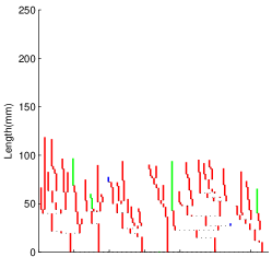
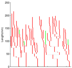
Figure 3.1: Example of a geodesic between artery trees showing five points along the geodesic. Blue edges are only in the tree of the first subject, red only in the other subject and green are common to both (pendants are not included in this visualization). The drastic dip along the geodesic path is characteristic for pairs of artery trees from this data set.

The artery tree Fréchet mean being degenerate is not an anomalous case. Theory about the behavior of Fréchet sample mean will be discussed in Ch. 4, in which the focus is formal study of the tendency for Fréchet means to be degenerate in treespace. In the next section we explore how the Fréchet mean varies over the range of treespace embeddings using 3 to all 128 landmarks.

3.2   Reduced landmark analysis

Nested subsets of landmarks are used in a hierarchical approach to studying the variability of vascular geometry with respect to the cortical surface across this sample. Here we study the effect of decreasing the number of landmarks on the Fréchet mean, the sample statistic which describes the center of the distribution.

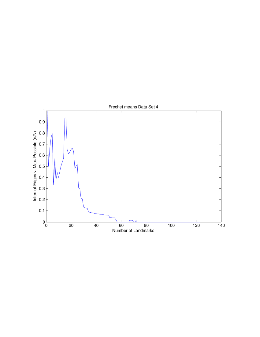
Figure 3.2: Ratio of number of interior edges versus maximal possible number of edges in Fréchet means as a function of increasing the number of landmarks.

The Fréchet means for tree representations using 3 up to 128 landmarks are calculated. Fig. 3.2 shows the ratio of the number of interior edges out of the maximum possible. Notice that in many cases the Fréchet mean has a highly degenerate topology, with the number of interior edges dropping off steadily when around 24 landmarks are used.

Rather than visualize the entire sequence of Fréchet mean trees we select a few interesting ranges for discussion. The ratio for the number of interior edges out of the maximum possible, as shown in Fig. 3.2, jumps up and down in the range from 3 landmarks to 12 landmarks, and steadily climbs up until reaching 18 landmarks. The Fréchet means for 6, 7, 8, and 9 landmarks are in Fig. 3.3 (on the next page). There we can see the pattern of edge contractions and expansions. Notice that the pair of landmarks 17 and 49 are stable in this range. Views of the trees in the range from 15 to 18 landmarks are in Fig. 3.4, there we can see that although the ratio of interior edges to maximal possible is steadily increasing there are both edges contracting and expanding in this range as well, though relatively fewer edges are contracting.

The small increase from zero interior up to 1 edge, at 69 landmarks is noteworthy. In fact the same interior edge is present in the Fréchet mean using 69, 70, 71 and 74 landmarks. It is suprising that this split isn’t in the Fréchet mean for 72 or 73 landmarks. Moreover, this split has a length of about 2mm in all four of those cases. This deserves further investigation. It either suggests that the lengths of edges which are incompatible with this split are fluctuating up and down in the range 69 to 74, or that this split is present in the Fréchet mean for 72 and 73 edges, but Sturm’s algorithm did not capture this feature before the search terminated. This line of investigation will be pursued in future research.

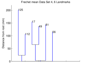
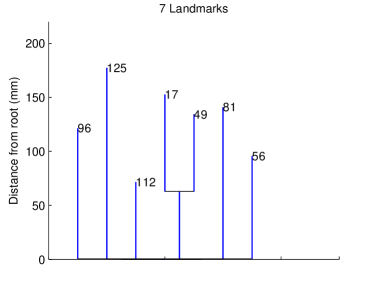
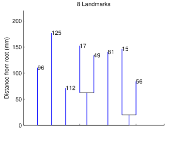
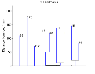
Figure 3.3: Tree views for the Frechet means for data sets having 6, 7, 8, and 9 landmarks.

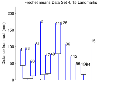
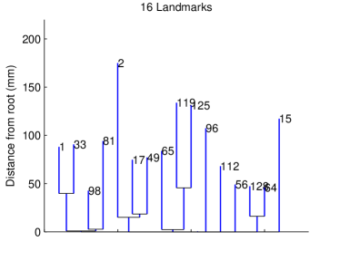
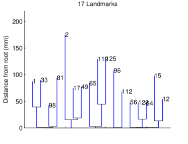
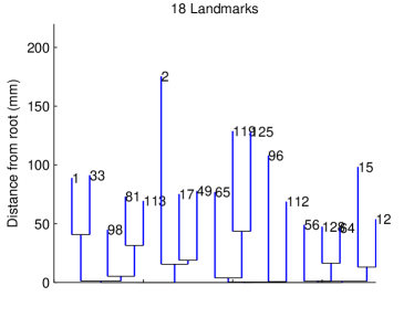
Figure 3.4: Tree views for the Frechet means for data sets having 15, 16, 17, and 18 landmarks.

The tendency of the Fréchet mean to be degenerate can be attributed to incompatible edges in among the data trees. Such incompatible edges represent that the artery system infiltrates regions near landmarks in topologically variable ways.

In the next chapter we take a theoretical approach to understanding the general behavior of Fréchet means in treespace.

CHAPTER 4: Fréchet means and stickiness

4.1   Introduction

In the analysis of brain artery systems in Ch. 3 we observed that the Fréchet mean becomes increasingly degenerate as the number of landmarks increases. Stickiness describes a finer point, which is that not only is the topology of the sample mean tree degenerate, but that if the sample is large enough then the topology of the sample mean is stable at the topology of the population mean when data points are added or removed from the sample.

Denote by $F_{n}(X)$ and $\bar{T}_{n}$ the Fréchet function and the Fréchet mean for a sample of $n$ independent and identically distributed observations on BHV treespace, $T^{1},T^{2},\ldots,T^{n}$, as defined in Sec. 2.1.1. The focus of this chapter is the probability distribution of $\bar{T}_{n}$ that is the Fréchet mean sampling distribution for $n$ observations. The main result Thm. 4.4.1 is a sticky law of large numbers for sampling distributions of Fréchet means on BHV treespace.

In treespace, depending on the population, the Fréchet mean sampling distribution can and often will exhibit the unusual property of stickiness. Contrasting the typical behavior of sample means, in most contexts small changes in the data result in small changes in the sample mean, but stickiness refers to the phenomenon of a sample mean which does not respond to small changes in the data. More precisely stickiness refers to the tendency of a sampling distribution to be fully supported on a lower dimensional subset of the sample space than the population distribution.

Definition 4.1.1.

A probability measure on treespace, $\mathcal{T}_{r}$, is said to to have a sticky Fréchet mean, $\bar{T}$, if $\bar{T}$ is degenerate and for every point $T$ in $\mathcal{T}_{r}$ there exists some $\alpha>0$ such that the topology of $\bar{T}$ is the same when the probability mass at $T$ is increased by up to $\alpha$.

Motivated to theoretically quantify stickiness, researchers have characterized the limiting distributions of sample means in BHV treespaces with 5 or fewer leaves Barden et al., (2013) and open books Hotz et al., (2012) with sticky central limit theorems. Sticky central limit theorems

• state the existence of a random finite sample size $N$ such that for sample sizes beyond $N$ the sample means stick with probability 1 ( $N$ quantifies the intensity of stickiness); and

• characterize the limiting sampling distribution on its support.

The remaining contents of this chapter are as follows. Sec. 4.2 summarizes existing results for stickiness of sampling distributions on $\mathcal{T}_{3}$. Sec. 4.3 mathematically describes probability measures on BHV treespace and further characterizes the notion of a sticky Fréchet mean. Sec. 4.4 contains the main result of this chapter, a sticky law of large numbers for sampling distributions of Fréchet means for population distributions spread over a negatively curved region of treespace.

4.2   Stickiness for Fréchet means on $\mathcal{T}_{3}$

The space $\mathcal{T}_{3}$ of phylogenetic trees with index set $\{0,1,2,3\}$ with pendant lengths included, as depicted in Fig. 4.1, is equivalent to an open half-book. This space is composed of three copies, $L_{1},L_{2},L_{3}$ of $\mathbb{R}^{5}_{\geq 0}$, called pages, pasted together on a four dimensional face, $L_{0}$, called the spine. For more details about the construction of phylogenetic treespaces see Sec. 1.2.3. Each page of the book corresponds to one of the three possible tree topologies, and the spine corresponds to the star tree topology. Let $L_{k}^{+}=L_{k}\setminus L_{0}$ be the portion of the $k^{th}$ page which is disjoint from the spine. Thus, $\mathcal{T}_{3}$ can be formed by a disjoint partition of the pages and spine, as $L_{0}\cup L_{1}^{+}\cup L_{2}^{+}\cup L_{3}^{+}$.

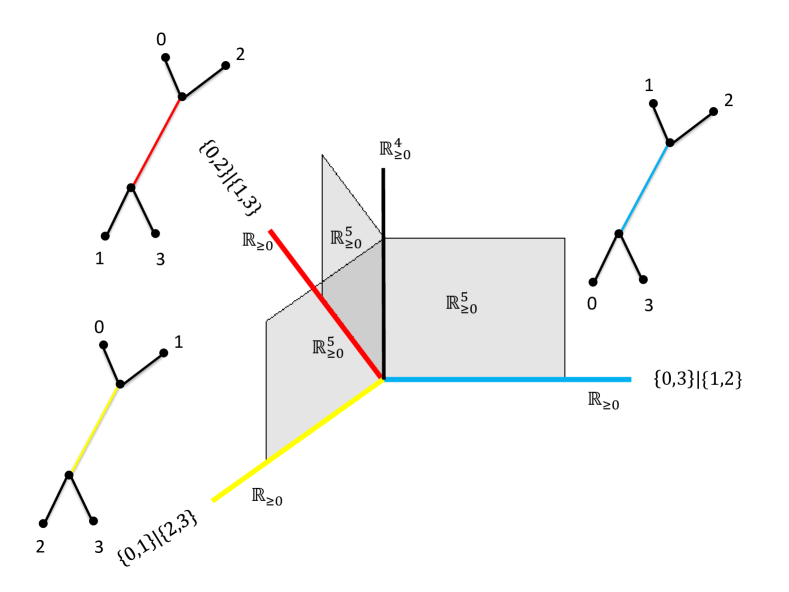
Figure 4.1: Depiction of $\mathcal{T}_{3}$: three copies of $\mathbb{R}^{5}_{\geq 0}$, $L_{1},L_{2},L_{3}$, each corresponding to one of three possible tree topologies pasted together on a copy of $\mathbb{R}^{4}_{\geq 0}$, denoted $L_{0}$.

The sticky law of large numbers for open books (Hotz et al.,, 2012, Thm. 4.3), is restated in this section for the special case of $\mathcal{T}_{3}$. Assume $T^{1},...,T^{n}$ are independently sampled from a probability measure, i.e. distribution, $\mu$ that is square-integrable and has spositive mass on each of $L_{1}^{+},L_{2}^{+},L_{3}^{+}$.

Definition 4.2.1.

The first moment of $\mu$ on the $k^{th}$ page is the real number

$$m_{j}=\int_{L_{j}^{+}}xd\mu(x)-\sum_{i\neq j}\int_{L_{k}^{+}}xd\mu(x).$$

Theorem 4.2.2.

(Hotz et al.,, 2012, Thm. 2.9) Assuming $\mu$ is square integrable and has positive mass on each page, the moments $m_{j}$, $j=1,2,3$ are either
1. (sticky) $m_{j}<0$ for all $j\in\{1,2,3\}$,
or there is exactly one index $k\in\{1,2,3\}$ such that $m_{k}\geq 0$, in which case either
2. (non-sticky) $m_{k}>0$, or
3. (partly sticky) $m_{k}=0$.

Let $\bar{T}=\operatorname{argmin}_{X\in\mathcal{T}_{3}}\int_{\mathcal{T}_{3}}d(X,T)^{2}d\mu(T)$.

Theorem 4.2.3.

($\mathcal{T}_{3}$ Sticky LLN) (Hotz et al.,, 2012, Thm. 4.3)

• If the moment $m_{j}$ satisfies $m_{j}<0$, then there is a random integer $N$ such that $\bar{T}_{n}\notin L_{j}^{+}$ for all $n\geq N$ with probability 1. Furthermore $\bar{T}\notin L_{j}^{+}$.

• If the moment $m_{k}$ satisfies $m_{k}>0$, then there is a random integer $N$ such that $\bar{T}_{n}\in L^{+}_{k}$ for all $n\geq N$ with probability 1. Furthermore $\bar{T}\in L_{k}^{+}$.

• If the moment $m_{k}$ satisfies $m_{k}=0$, then there is a random integer $N$ such that $\bar{T}_{n}\in L_{k}$ for all $n\geq N$ with probability 1. Furthermore, $\bar{T}\in L_{0}$.

The focus in the proceeding sections is a Sticky LLN for $\mathcal{T}_{3}$. Analysis leading to a Sticky LLN for $\mathcal{T}_{r}$ in general is facilitated by a slight change of tack. The analysis for open books uses the moments $m_{k}$ to precisely describe the conditions of stickiness. A comment, in (Hotz et al.,, 2012, Rem. 2.11) which states that $m_{k}$ is a directional derivative of the Fréchet function from the spine into the $k^{th}$ page, can be used to formulate an equivalent characterization of stickiness. Sec. 2.4 gives a detailed analysis of directional derivatives from lower dimensional faces into higher dimensional faces of $\mathcal{T}_{r}$, which play analogous roles to directional derivatives from the spine into pages of $\mathcal{T}_{3}$. The next section describes probability measures on BHV treespace, and characterizes levels of stickiness for the Fréchet mean of a probability measure.

4.3   Fréchet means for probability measures on treespace

Suppose that $\mu$ is a probability measure on BHV treespace, $\mathcal{T}_{r}$. Let $0$ denote the origin of $\mathcal{T}_{r}$. Assume that the distance between $0$ and $T\in\mathcal{T}_{r}$, $d(0,T)$ has bounded expectation under the measure $\mu$:

$$\displaystyle\int_{\mathcal{T}_{r}}d(0,T)d\mu(T)<\infty.$$ (4.1)

BHV treespace can be partitioned into disjoint open orthants, each corresponding to a unique phylogenetic tree topology. Any probability measure $\mu$ on $\mathcal{T}_{r}$ decomposes uniquely as a weighted sum of probability measures $\mu_{\mathcal{O}}$ on the open orthants of BHV treespace. Therefore there are non-negative numbers $\{w_{\mathcal{O}}\}$ summing to 1 such that for any Borel set $A\subseteq\mathcal{T}_{r}$, the measure $\mu$ takes the value

$$\mu(A)=\sum_{\mathcal{O}}w_{\mathcal{O}}\mu_{\mathcal{O}}(A\cap\mathcal{O}).$$ (4.2)

The Fréchet function for a probability measure $\mu$ is

$$\displaystyle F_{\mu}(X)=\int_{\mathcal{T}_{r}}{d^{2}(X,T)}d\mu(T)$$ (4.3)

The Fréchet function is strictly convex and its minimizer is the Fréchet mean, $\bar{T}$ Sturm, (2003)[Prop. 4.3].

Properties for directional and partial derivatives for the Fréchet function for a probability measure $\mu$ follow a development similar to the properties for the Fréchet function for a sample as in Ch. 2. Thus we state their key properties now without detailed proofs.

Let $T$ be a tree, let $X$ be a variable point, Let $Y$ be a tree such that $\mathcal{O}(X)\subseteq\mathcal{O}(Y)$ such that $X$ and $Y$ share a multi-vistal cell. Let $(A_{1},B_{1}),\ldots,(A_{k^{T}},B_{k^{T}})$ be a support for the geodesic from $Y$ to $T$. Let $(A_{1},B_{1}),\ldots,(A_{m^{T}},B_{m^{T}})$ be local support pairs, and let $(A_{m^{T}+1},B_{m^{T}+1}),\ldots,(A_{k^{T}},B_{k^{T}})$ be the rest of the geodesic support sequence being used to represent the geodesic between $Y$ and $T$. The restricted gradient of the Fréchet function in the minimal orthant containing $X$ is

$$[\nabla F_{\mu}(X)]_{e}=2\int_{\mathcal{T}_{r}}\left\{\begin{array}[]{ll}\left(1+\frac{\lVert B_{l}\rVert_{T}}{\lVert A_{l}\rVert_{X}}\right)|e|_{X}&\textrm{if $e\in A_{l}$}\\ \left(|e|_{X}-|e|_{T}\right)&\textrm{if $e\in C$}\end{array}\right\}d\mu(T).$$ (4.4)

if $|e|_{X}>0$ and $0$ otherwise. Let $p_{e}=|e|_{Y}-|e|_{X}$ for all $e\in E_{Y}$. The directional derivative of the Fréchet function for probability measure $\mu$ from $X$ in the direction $Y$ is

$$F_{\mu}^{\prime}(X,Y)=\sum_{e\in E_{X}}p_{e}[\nabla F_{\mu}(X)]_{e}+\int_{\mathcal{T}_{r}}\left(\sum_{l=1}^{m^{T}}{2\lVert B_{l}\rVert_{T}\sqrt{\sum_{e\in A_{l}}{p_{e}^{2}}}}+\sum_{e\in C^{T}\cap S}{-2p_{e}|e|_{T}}\right)d\mu(T).$$ (4.5)

The directional derivative decomposes the sum of the directional derivative along the component $Y_{X}$ of $Y$ in $\mathcal{O}(X)$ and the component $Y_{\perp}$ of $Y$ which is perpendicular to $\mathcal{O}(X)$

$$F^{\prime}_{\mu}(X,Y)=F^{\prime}_{\mu}(X,Y_{X})+F^{\prime}_{\mu}(X,Y_{\perp}).$$ (4.6)

A point $X$ is the Fréchet mean of $\mu$ if and only if it satisfies the Fréchet optimality conditions

$$[\nabla F_{\mu}(X)]_{e}=0 \;\;\;\forall\;e\in E_{X}$$ (4.7)

$$F_{\mu}^{\prime}(X,Y)\geq 0 \;\;\;\forall\;Y\textrm{ s.t. the component of $Y$ in $\mathcal{O}(X)$ is 0}.$$ (4.8)

The Fréchet mean, $\bar{T}$, for a measure $\mu$ is either

• sticky on the minimal open orthant containing $\bar{T}$ if $F_{\mu}^{\prime}(\bar{T},Y)>0$ for all $Y$ which are perpendicular to $\mathcal{O}(\bar{T})$ at $\bar{T}$,

• partially sticky on the minimal open orthant containing $\bar{T}$ if $F_{\mu}^{\prime}(\bar{T},Y)\geq 0$ for all $Y$ which are perpendicular to $\mathcal{O}(\bar{T})$ at $\bar{T}$ and $F^{\prime}(\bar{T},Y)=0$ for some $Y$ which is perpendicular to $\mathcal{O}(\bar{T})$ at $\bar{T}$, or

• non-sticky if $\bar{T}$ is non-degenerate.

Lemma 4.3.1.

If $\mu$ is partially sticky, then the set of $Y$ s.t. $F_{\mu}^{\prime}(\bar{T},Y)=0$ is a convex subset of treespace.

Proof.

The directional derivative $F_{\mu}^{\prime}(\bar{T},Y)$ is a convex function of $Y$ for $Y$ in a small neighborhood of $\bar{T}$. The level set $\{Y|F_{\mu}^{\prime}(\bar{T},Y)\leq 0\}$ is a convex set and there are no $Y$ such that $F_{\mu}^{\prime}(\bar{T},Y)<0$. ∎

4.4   LLN for sample means in BHV treespace

This section starts out by stating a classical strong law of large numbers for $\mathcal{T}_{r}$ which is a special case of the strong law of large numbers introduced in Sturm, (2003) for metric spaces of non-positive curvature, of which treespace is a special case. The novel result in this section is that sample means in BHV treespace obey a sticky law of large numbers.

Theorem 4.4.1.

(Strong Law of Large Numbers). There is a unique point $\bar{T}\in\mathcal{T}_{r}$ such that

$$\lim_{n\to\infty}\bar{T}_{n}=\bar{T}$$

holds with probability one. The point $\bar{T}$ is the Fréchet mean of $\mu$.

Proof.

This is a special case of (Sturm,, 2003, Prop. 6.6) which gives a Strong Law of Large Numbers for distributions on globally non-positively curved metric spaces. ∎

The treespace Strong LLN (Thm. 4.4.1) guarantees, that for any $\epsilon>0$, there exists a finite integer $N$ such that for all $n>N$, $d(\bar{T}_{n},\bar{T})<\epsilon$. This guarantees that for large enough samples, every $e\in E_{\bar{T}}$ close to its length in $\bar{T}$, and that if $\bar{T}$ is degenerate then any edges in $\bar{T}_{n}$ which are not in $E_{\bar{T}}$ must have lengths which are bounded above by $\epsilon$. The following Sticky LLN specifies that when $\bar{T}$ is degenerate then for large enough samples the Fréchet sample mean, $\bar{T}_{n}$, will not contain any edges which are not in $\bar{T}$.

Theorem 4.4.2.

(Sticky Law of Large Numbers)

• Sticky case: If $F^{\prime}(\bar{T},Y)>0$ for all $Y$ which are perpendicular to $\mathcal{O}(\bar{T})$ at $\bar{T}$ then there exists a random integer $N$ such that for all $n>N$, $F^{\prime}_{n}(X,Y)>0$ for all $Y$ which are perpendicular to $\mathcal{O}(\bar{T})$ and $E_{\bar{T}_{n}}=E_{\bar{T}}$.

• Partially sticky case: If $F^{\prime}(\bar{T},Y)\geq 0$ for all $Y$ in the normal space of $\bar{T}$ and $F^{\prime}(\bar{T},Y)=0$ for some $Y$ in the normal space of $\bar{T}$ then there exists a random integer $N$ such that for all $n>N$, if $F^{\prime}(\bar{T};Y)>0$ then $F^{\prime}(X,Y)>0$, and if $F^{\prime}(\bar{T};Y)=0$ then the sample mean $\bar{T}_{n}$ has a positive probability of being in $\mathcal{O}(Y)$.

• Non-sticky case: If $\bar{T}$ is non-degenerate then there exists a random integer $N$ such that for all $n>N$ $E_{\bar{T}_{n}}=E_{\bar{T}}$.

Proof.

The treespace Strong Law of Large Numbers (Thm. 4.4.1 guarantees the existence of a finite integer $N$ such that for all $n>N$, $|e|_{\bar{T}_{n}}>0$ for all $e\in E_{\bar{T}}$.

Next we show that there must exist some finite integer $N$ such that for all $n>N$, $|e|_{\bar{T}_{n}}=0$ for all $e$ such that $|e|_{\bar{T}}=0$. Essentially the proof is based on the Fréchet optimality conditions. Let $X$ be a point in $\mathcal{O}(\bar{T})$. For every $Y$ such that the component of $Y$ in $\mathcal{O}(\bar{T})$ is zero the values of the directional derivatives $F^{\prime}_{\mu}(X,Y)$ and $F^{\prime}_{n}(X,Y)$ are independent of the precise edge lengths of $X$, provide that every edge in $\mathcal{O}(\bar{T})$ has a positive length. We show the directional derivative $F^{\prime}_{n}(X,Y)$ for $Y$ perpendicular to $\mathcal{O}(\bar{T})$ approaches $F^{\prime}_{\mu}(X,Y)$ with probability 1. for any $X\in\mathcal{O}(\bar{T})$. This will suffice to prove the claim since we have already established that $E_{\bar{T}}\subseteq E_{\bar{T}_{n}}$ using the Strong Law of Large Numbers.

Consider a point in the minimal open orthant containing the Fréchet mean, $X\in\mathcal{O}(\bar{T})$, and a point $Y$ such that the component of $Y$ in $\mathcal{O}(\bar{T})$ is zero. Since the component of $Y$ in $\mathcal{O}(\bar{T})$ is zero

$$F^{\prime}_{n}(X,Y)=\frac{1}{n}\sum_{i=1}^{n}\left(\sum_{l=1}^{m^{i}}{2\lVert B^{i}_{l}\rVert\sqrt{\sum_{e\in A^{i}_{l}}{p_{e}^{2}}}}+\sum_{e\in C^{i}\cap S}{-2p_{e}|e|_{T^{i}}}\right)$$

Treespace $\mathcal{T}_{r}$ can be subdivided into a disjoint set of the open interiors of vistal cells such that for each vistal cell $\mathcal{V}$, the geodesic from $Y$ to any $T$ in $\mathcal{V}$ can be represented with the same combinatorial form. Thus the directional derivative from $X$ to $Y$ can be separated into a sum of terms each contributed by a vistal cell $\mathcal{V}$. Let $1_{T\in\textrm{int}(\mathcal{V})}$ be an indicator function with value 1 if $T\in\textrm{int}(\mathcal{V})$ and 0 otherwise.

$$F^{\prime}_{n}(X,Y)=\sum_{\mathcal{V}}\left(\sum_{i=1}^{n}\left(1_{T^{i}\in\textrm{int}(\mathcal{V})}\frac{1}{n}\sum_{l=1}^{m^{i}}\left({2\lVert B^{i}_{l}\rVert\sqrt{\sum_{e\in A^{i}_{l}}{p_{e}^{2}}}}\right)+\sum_{e\in C^{i}\cap S}{-2p_{e}|e|_{T^{i}}}\right)\right)$$ (4.9)

For a fixed $\mathcal{V}\subseteq\mathcal{O}$, each $T^{i}\in\mathcal{V}$ is equivalent to a random vector in $\mathcal{O}$; thus by the classical Law of Large Numbers (Shapiro et al.,, 2009, Sec. 7.2.5)

$$\lim_{n\to\infty}\frac{1}{n}\sum_{i=1}^{n}\left(1_{T^{i}\in\textrm{int}(\mathcal{V})}\sum_{l=1}^{m^{i}}\left({2\lVert B^{i}_{l}\rVert\sqrt{\sum_{e\in A^{i}_{l}}{p_{e}^{2}}}}\right)+\sum_{e\in C^{i}\cap S}{-2p_{e}|e|_{T^{i}}}\right)$$ (4.10)

$$=\mu(\textrm{int}(\mathcal{V}))\int_{\textrm{int}(\mathcal{V})}\left(\sum_{l=1}^{m^{T}}{2\lVert B_{l}\rVert_{T}\sqrt{\sum_{e\in A_{l}}{p_{e}^{2}}}}+\sum_{e\in C^{T}\cap S}{-2p_{e}|e|_{T}}\right)d\mu_{\textrm{int}(\mathcal{V})}(T)$$ (4.11)

with probability 1. Hence, by summing over all vistal cells,

$$\lim_{n\to\infty}F^{\prime}_{n}(X,Y)\to F^{\prime}_{\mu}(X,Y)$$ (4.12)

with probability 1. ∎

4.4.1   Extensions

In treespace and the open book, where stickiness has been observed and studied theoretically, the population is distributed on a negatively curved region of the sampling space. It is conjectured that positively curved geometry leads to “antistickiness” and negatively curved geometry leads to “stickiness” Hotz et al., (2012). Although the topic of antistickiness is not explored any further here, it may be a topic of future research. The 2-dimensional sphere would be an ideal model space to study antistickiness phenomenon for sample means on positively curved metric spaces. There may also be theoretical connections between robust estimation, sparse estimation, and stickiness, although investigating these connections is outside of the scope of this thesis.

It is plausible that sticky central limit theorems will generalize to any dimension of treespace because they all share the property of global non-positive curvature. The sticky LLN here is a precursor for a central limit theorem because it characterizes the limiting distribution as sticky i.e. characterizes the support of the limiting distribution. In this sense this result further justifies the conjecture that sticky central limit theorems are generalizable to any dimension of treespace. A sticky central limit theorem for samples on BHV treespace would be an interesting topic for further research.

CHAPTER 5: Treespace kernel smoothing

5.1   Introduction

One way that methods for statistical analysis of populations of complex objects e.g. tree-structured data, functional data, and manifold data, can contribute to biological sciences, such as neuroscience and developmental biology, is through the use of flexible models for studying trends in parts of anatomy. The motivation of this chapter is to study the variation in branching and geometry of 3D anatomical trees as a function of age. In particular, in this chapter, Fréchet kernel smoothing of brain artery trees over age is introduced for analysis of the CASILab cross-sectional dataset of human brain artery systems described in Ch 1.

Kernel smoothing of tree-structured data objects was first studied in Wang et al., (2011). The findings in that paper serve as a motivation to continue studying non-parametric regression for tree-structured data. In that paper they found an increase in common structure among 20 to 30 year old subjects, and a decrease in common structure among 30 to 50 year old subjects. The method in that paper is based on connectivity only, and the goal of this chapter is to obtain deeper insights by including additional structural information in the tree-data object representation.

The approach in this chapter, and that previous approach, both use the framework of kernel smoothing (see Fan and Gijbels, (1996); Härdle, (1991); Wand and Jones, (1994) for books on kernel smoothing), but differ in their representations of artery systems, and thus in their choice of metric. The previous work represents artery systems as binary trees, which are purely topological objects. It uses the integer tree metric, which counts the total number of non-common nodes between two trees Wang and Marron, (2007). In this chapter artery systems are represented as points in BHV treespace. This representation captures the topological structure of the entire tree and lengths of individual artery segments.

The organization of the rest of this chapter is as follows. In Sec. 5.2, a novel method for kernel smoothing of data points which have tree-structured response, and predictive values in a Euclidan space is presented. In Sec. 5.3 we present a case study of the sample of human brain artery systems of normal adults collected at the UNC Chapel Hill CASILab discussed in Sec. 1.3. Sec. 5.4 is an appendix for descriptions of algorithms used in this research.

5.2   Methodology

5.2.1   Treespace Kernel Smoothing

Consider a dataset of bivariate observations $(x_{1},T^{1}),\ldots,(x_{n},T^{n})$, where $x_{1},\ldots,x_{n}$ are explanatory observations in $\mathbb{R}$ and $T^{1},\ldots,T^{n}$ are dependent observations in a BHV treespace, $\mathcal{T}$. Kernel smoothing can be used to study the relationship between explanatory and dependent variables in a flexible way.

A weighting for a dataset is an assignment of a weight, a positive real number $w_{i}$, to each observation $i=1,\ldots,n$, such that $\sum w_{i}=1$. In the context of smoothing, a kernel $K$ is a function used to create weightings. A kernel takes as input two points $x$ and $x^{\prime}$ in the space of explanatory variables. The operations of the kernel are (1) calculate the distance between $x$ and $x^{\prime}$, (2) scale their distance by division by the band width parameter $h$, and (3) pass the scaled distance into a non-negative, symmetric window function $D$. In summary a kernel function is

$$K(x,x^{\prime};h)=D\left(\frac{\lVert x-x^{\prime}\rVert}{h}\right)$$

For kernel $K$ and bandwidth $h$, at a given point $x$, the kernel-weight function assigns a weight to observation $i$

$$w_{i}(x)=\frac{K(x,x_{i};h)}{\displaystyle\sum_{i}K(x,x_{i};h)}$$

Here, a Gaussian density function is used for the kernel. The weighted Fréchet function $F:{\mathcal{T}}\to\mathbb{R}_{\geq 0}$, which generalizes the Fréchet function introduced in Ch. 2, is a sum of weighted mean squared distances

$$F(T;w)=\sum_{i=1}^{n}{w_{i}d(T,T^{i})^{2}}.$$

Following a development parallel to methods for Fréchet means, the unique minimizer of the weighted Fréchet function is called the weighted Fréchet sample mean

$$\bar{T}(w)=\operatorname{argmin}_{T\in{\mathcal{T}}}{F(T;w)}.$$

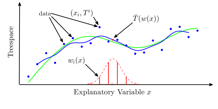
Figure 5.1: Schematic of Fréchet kernel smoothing. Data are blue dots, a noisy sample from the green curve; the red dashed curve is a Gaussian kernel function and the vertical bars represent the relative weights of data points; red dot is kernel weighted mean at $x$, $\bar{T}(w(x))$; and the blue curve is the kernel smooth.

Fig. 5.1 shows a schematic of Fréchet kernel smoothing. There we can see how an estimate for the response value at the point $x$ is created using a local Fréchet mean.

The results of kernel smoothing are dependent on the bandwidth $h$. When $h$ is very small, the weights are concentrated on data points within a narrow range, and the smoothed values are very localized. An extreme case, when $h=0$, results in local estimates which are either empty or just the data points themselves. At the other extreme, when the bandwidth is very large, all data points have very similar weights, and the smoothed tree for any value $x$ is very similar to the overall Fréchet mean of the dataset.

The bandwidth parameter, $h$, in classic nonparametric regression, is selected to optimize some expected error, or its empirical (e.g. cross-validation) or asymptotic estimate. See Fan and Gijbels, (1996); Härdle, (1991); Wand and Jones, (1994) for detailed descriptions of such techniques. A scale space approach to the bandwidth selection problem, which compares smooths across a range of window sizes to look for consistent patterns as recommended in Chaudhuri and Marron, (1999), is used here.

Adapting the optimization algorithms from Ch. 2 to solve for a weighted Fréchet mean $\bar{T}(w)$ is straightforward. The step length in each iterative step of a cyclic split proximal point algorithm can be modified to account for the weight, $w_{i}$, on each term in the Fréchet sum of squares. For a random split proximal point algorithm (a.k.a Sturm’s algorithm), the probability of sampling a data point, $T^{i}$, at each iteration is equal to its weight, $w_{i}$. For descent methods, the only changes come from appropriately multiplying terms in the Fréchet function and its derivatives by the weights, $w_{1},\ldots,w_{n}$.

5.2.2   Methods for summarizing treespace smooths

Summarizing treespace smooths is a critical step in studying the relationship between predictive and response variables. Key summaries of each tree, such as the total number of interior edges, and the sum of interior edge lengths are just the first step. Comparing these summaries across smoothing bandwidths can provide insights into the data. But these comparisons are somewhat limited in that they don’t capture topological variation across the smooth. Tree topologies are discussed in the introduction to phylogenetic trees in Sec. 1.2.

5.2.2.1 Minimum Length Representative Sequences

Summarizing length and number of edges does not capture the variation in tree topologies in a tree-smooth. While counting the number of edges quantifies degeneracy, it does not consider the variety of splits in tree topologies across the smooth. Thus the aim here is to summarize the topological variability in an ordered set of trees.

For a set of trees $T^{1},\ldots,T^{n}$ a representative tree topology, $R$, is a tree topology such that every element, $T^{i}$, has a subset of the edges in the topology $R$. A representative tree topology may not exist for an arbitrary set of trees. For $T^{1},\ldots,T^{n}$, a representative set of tree topologies, $R^{1},\ldots,R^{k}$, has the property that every element $T^{i}$ has a subset of the edges in topology $R^{j}$ for some $j$. For an ordered set of trees $T^{1},\ldots,T^{n}$ a representative sequence is a sequence of tree topologies $R^{1},\ldots,R^{k}$ such that $R^{1}$ is a representative tree topology for the first $i_{1}$ trees, $T^{1},\ldots,T^{i_{1}}$, $R^{2}$ is a representative tree topology for the next $i_{2}$ trees, $T^{i_{1}+1},\ldots,T^{i_{2}}$, and so on. A minimum length representative sequence is a representative sequence with the fewest number of representative tree topologies possible. An algorithm for finding a minimum length representative sequence is in the last section of this chapter, Sec. 5.4.

In data analysis, a minimum length representative sequence for the predicted response trees in a tree-smooth will be used to capture the variety of tree topologies over the range of the predictive variable.

5.3   Case study of CASILab angiography dataset

In Ch. 3 we studied how the ratio of interior edges to the maximum possible number of interior edges varied over reduced sets of landmarks. When this ratio is close to 1 it indicates a relatively higher degree of common structure. In this analysis, we will work with 17 landmarks because of the relatively high degree of common structure.

This data set contains 85 subjects with ages approximately uniformly distributed in the range 20 to 80 years. Because the density of observations affects the results a closer look at the distribution of ages will make for a more informed analysis. As we can see in Fig. 5.2, there are only 2 subjects over 70. While we will use all the available data in the analysis, due to the sparsity of data over 70, we will not attempt to make any estimates in that range.

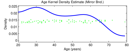
Figure 5.2: Kernel density estimate for distribution of subject ages.

A Gaussian probability density is used for the kernel window function. The effect of scale is studied across six smoothing levels: $h=1,2,3,4,5,6$ years. In this data analysis, the kernel estimator will be evaluated at the ages from data points. These point estimates are adequate to study the relationship between artery trees and ages.

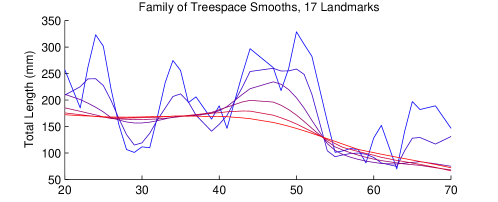
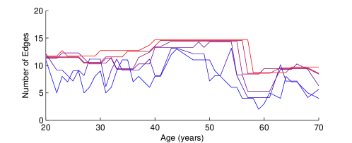
Figure 5.3: Summaries from treesmooth family with bandwidths $h=1,2,3,4,5,6$ colored from blue to burgundy to red. Sum of lengths of interior edges over age (top); and number of interior edges over age.

Now we begin discussing the results. We discuss the results in terms of two key summaries of treesmooths, the sum of interior edge lengths and the number of interior edges. Then we study the topological variability across ages as summarized by minimum length representative sequences.

Fig. 5.3 displays the sum of the interior edge lengths (top) and the number of interior edges. Notice that for the total length there is a clear overall downward trajectory which becomes increasingly evident as the bandwidth increases. This is consistent with a previous study, which showed a significant decrease in total length of the entire artery system with age Skwerer et al., (2014). Fluctuations in total length for smooths using narrower windows, $h=1,2,3$, colored blue to purple in Fig. 5.3, are positively correlated with fluctuations in the number of edges. This pattern is shown clearly in the scatterplots of number of edges and total length in Fig. 5.4. For smoothing levels $h=4,5,6$, burgundy to red, a striking pattern in the scatterplots emerges. The line of trees along the top of the plot coincides with the flat segment over the range of 40 to 55 years in Fig. 5.3. We will offer a further interpretation for this pattern in our discussion of topological variability across the smooth.

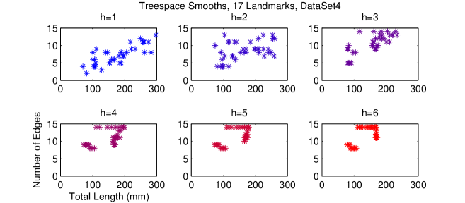
Figure 5.4: Scatter plots of number of interior edges and total length for smoothing windows $h=1,2,3,4,5,6$ years with the same colors as Fig. 5.3. We see a positive correlation between these variables indicating that their up and down fluctuations across ages coincide.

For summarizing the topologies across the smooth we use a minimum length representative sequence as described in Sec. 5.2.2.1. Smoothing dramatically decreases the length of the minimum representative sequence. The sequence of data trees $T^{1},\ldots,T^{85}$, ordered by ages, $x_{1},\ldots,x_{85}$ are their own minimal length representative sequence. The number of representative topologies by smoothing bandwidth are summarized in Table 5.1.

$h$ yrs	# Top.
0	85
1	7
2	2
3	2
4	1
5	1
6	1

Table 5.1: Number of topologies in the minimal representative sequence for each smoothing window.

The representative topology is the same for bandwidths $h=4,5,6$. In fact this representative topology is the topology of the overall Fréchet mean of the entire dataset, shown in Fig. 5.5. The patterns we see in Fig. 5.3 and Fig. 5.4 represent the smooth trees varying between various degenerate trees that are contractions of this representative topology.

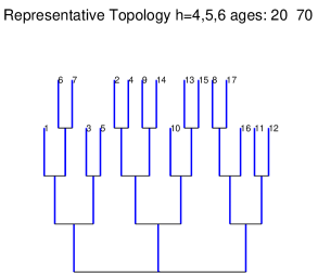
Figure 5.5: Representative topology for treespace smooths with bandwidths $h=4,5,6$. These bandwidths are large enough so the representative topology for the treesmooth is equal to the topology of the overall Fréchet mean.

For smoothing bandwidths $h=1,2,3$ several representative topologies are needed to capture different ranges of ages.

For bandwidth $h=2$ the first representative topology captures ages 20 to 38, and the second captures ages 39 to 68. For $h=3$ the first representative topology captures ages 20 to 39 and the second captures ages 40 to 68. The representative topologies are the same for bandwidths $h=2,3$; these are shown in Fig. 5.6, where we can see that the representative topology for ages 20 to 38 only has one edge which is not shared by the overall Fréchet mean, and the representative topology for ages 39 to 70 is the topology of the overall Fréchet mean.

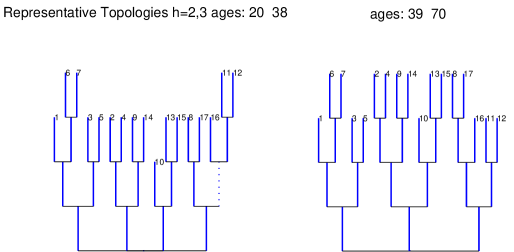
Figure 5.6: Representative topologies for treesmooths for both bandwidths $h=2,3$. The dotted edge in the left hand tree is the only edge which is not in the overall Fréchet mean.

For $h=1$ the first representative topology captures the topologies in the treesmooth for ages 20 to 24, the second captures ages 25 to 33, the third captures 34 to 42, the fourth captures 43 to 50, the fifth captures 51 to 52, the sixth captures 54 to 62 and the seventh captures 63 to 68.

5.4   Minimum Length Representative Sequence Algorithm

In this section we describe an algorithm to find a minimum length representative sequence for a sequence of trees $T^{1},\ldots,T^{n}$.

Let $R(i,1),\ldots,R(i,k^{i})$ be a minimum length representative sequence for $T^{1},\ldots,T^{i}$. When $i=1$ the minimum length representative sequence is $R(1,1)=T^{1}$.

Let $S(i,n)$ be a representative topology for $(T^{i+1},\ldots,T^{n}$) if a representative topology exists. Let $k^{0}=0$. Let $i^{*}$ be an non-negative integer which minimizes $k^{i}$ among all $i$ such that $S(i,n)$ exists.

Theorem 5.4.1.

A minimum length representative sequence for $T^{1},\ldots,T^{n}$ is

$$R(i^{*},1),\ldots,R(i^{*},k^{i*}),S(i^{*},n)$$ (5.1)

Proof.

The proof will be by contradiction. Suppose there exists representative sequence $R^{1},\ldots,R^{l}$ with length $l$ less than $k^{i*}+1$ for $T^{1},\ldots,T^{n}$. Suppose that $R^{l}$ is representative for $T^{j+1},\ldots,T^{n}$ then $R^{1},\ldots,R^{l-1}$ are a representative sequence for $T^{1},\ldots,T^{j}$ having length $l-1<k^{i*}$. But this is a contradiction because $k^{i*}$ must be less than or equal to the length of any representative sequence for $T^{1},\ldots,T^{j}$. ∎

REFERENCES

REFERENCES

- (1) Aydin, B., Pataki, G., Wang, H., Bullitt, E., and Marron, J. (2009a). A principal component analysis for trees.
- (2) Aydin, B., Pataki, G., Wang, H., Ladha, A., Bullitt, E., and Marron, J. (2009b). Visualizing the structure of large trees. Electron. J. Statist., 5:405–420.
- Aylward and Bullitt, (2002) Aylward, S. and Bullitt, E. (2002). Initialization, noise, singularities, and scale in height ridge traversal for tubular object centerline extraction. IEEE Transactions on Medical Imaging, 21:61–75.
- Barden et al., (2013) Barden, D., Le, H., and Owen, M. (2013). Central limit theorems for Fréchet means in the space of phylogenetic trees. Electronic Journal of Probability, 18:1–25.
- Bac̆àk, (2012) Bac̆àk, M. (2012). A novel algorithm for computing the fréchet mean in hadamard spaces. http://arxiv.org/pdf/1210.2145v1.pdf (2012).
- Bačák, (2012) Bačák, M. (2012). The proximal point algorithm in metric spaces. Israel Journal of Mathematics, 194(2):689–701.
- Bertsekas, (2011) Bertsekas, D. P. (2011). Incremental proximal methods for large scale convex optimization. Mathematical Programming, 129(2):163–195.
- Bullitt et al., (2008) Bullitt, E., Smith, J., and Lin, W. (2008). Designed database of MR brain images of healthy volunteers.
- Chaudhuri and Marron, (1999) Chaudhuri, P. and Marron, J. S. (1999). SiZer for Exploration of Structures in Curves. Journal of the American Statistical Association, 94(447):807–823.
- Fan and Gijbels, (1996) Fan, J. and Gijbels, I. (1996). Local Polynomial Modelling and Its Applications: Monographs on Statistics and Applied Probability 66. CRC Press.
- Feragen et al., (2012) Feragen, A., Lo, P., de Bruijne, M., Nielson, M., and Lauze, F. (2012). Towards a theory of statistical tree-shape analysis. IEEE Transactions on Pattern Analysis and Machine Intelligence, 20.
- Haeckel, (1866) Haeckel, E. (1866). Generelle Morphologie der Organismem: Allgemeine Grundzuge der organischen Forman-Wissenschaft, mechanisch begrundet durch die von Charles Darwin, reformite Descendenz-Theorie. Georg Riemer.
- Härdle, (1991) Härdle, W. (1991). Applied Nonparametric Regression. Cambridge University Press.
- Harris, (1952) Harris, T. (1952). First passage and recurrence distributions. Transactions of the American Mathematical Society, 73:471–486.
- Hotz et al., (2012) Hotz, T., Huckemann, S., Le, H., Mattingly, J. M. J., Miller, E., Nolen, J., Owen, M., Patrangenaru, V., and Skwerer, S. (2012). Sticky central limit theorems on open books. Annals of Applied Probability.
- Li et al., (2009) Li, C., Lopez, G., and Martin-Marquez, V. (2009). Monotone vector fields and the proximal point algorithm on Hadamard manifolds. Journal of the London Mathematical Society, 79(3):663–683.
- Miller et al., (2012) Miller, E., Owen, M., and Provan, J. (2012). Polyhedral computational geometry for averaging metric phylogenetic trees. http://arxiv.org/abs/1211.7046.
- Oguz et al., (2008) Oguz, I., Cates, J., Fletcher, T., Whitaker, R., Cool, D., Aylward, S., and Styner, M. (2008). Cortical correspondence using entropy-based particle systems and local features. In Biomedical Imaging: From Nano to Macro, 2008. ISBI 2008. 5th IEEE International Symposium on Biomedical Imaging, pages 1637–1640. IEEE.
- Owen and Provan, (2009) Owen, M. and Provan, S. (2009). A fast algorithm for computing geodesic distances in tree space. Computational Biology and Bioinformatics, 8:2–13.
- Ramsay and Silverman, (2002) Ramsay, J. and Silverman, B. (2002). Applied Functional Data Analysis. Springer.
- Ramsay and Silverman, (2005) Ramsay, J. and Silverman, B. (2005). Functional Data Analysis. Springer.
- Rockafellar, (1976) Rockafellar, R. T. (1976). Monotone Operators and the Proximal Point Algorithm. SIAM Journal on Control and Optimization, 14(5):877–898.
- Shapiro et al., (2009) Shapiro, A., Dentcheva, D., and Ruszczyǹski, A. (2009). Lectures on Stochastic Programming: Modeling and Theory. SIAM.
- Shen et al., (2012) Shen, D., Shen, H., Shankar, B., Muoz Maldano, Y., Kim, Y., and Marron, J. (2012). Functional data analysis of tree data objects. Journal of Computational and Graphical Statistics.
- Skwerer et al., (2014) Skwerer, S., Bullitt, E., Huckemann, S., Miller, E., Oguz, I., Owen, M., Patrangenaru, V., Provan, S., and Marron, J. S. (2014). Tree-Oriented Analysis of Brain Artery Structure. Journal of Mathematical Imaging and Vision.
- Sturm, (2003) Sturm, K. (2003). Probability measures on metric spaces of nonpositive curvature, in heat kernels and analysis on manifolds, graphs, and metric spaces: lecture notes from a quarter program on heat kernels, random walks, and analysis on manifolds and graphs. 338:357–390.
- Wand and Jones, (1994) Wand, M. and Jones, M. (1994). Kernel Smoothing. CRC Press.
- Wang and Marron, (2007) Wang, H. and Marron, J. (2007). Object oriented data analysis: sets of trees. The Annals of Statistics, 35:1849–1873.
- Wang et al., (2011) Wang, Y., Marron, J., Aydin, B., Ladha, A., Bullitt, E., and Wang, H. (2011). A nonparametric regression model with tree-structure response. Journal of the American Statistical Association, 107:1272–1285.