Efficient Feature Group Sequencing for Anytime Linear Prediction

Abstract

We consider anytime linear prediction in the common machine learning setting, where features are in groups that have costs. We achieve anytime (or interruptible) predictions by sequencing the computation of feature groups and reporting results using the computed features at interruption. We extend Orthogonal Matching Pursuit (OMP) and Forward Regression (FR) to learn the sequencing greedily under this group setting with costs. We theoretically guarantee that our algorithms achieve near-optimal linear predictions at each budget when a feature group is chosen. With a novel analysis of OMP, we improve its theoretical bound to the same strength as that of FR. In addition, we develop a novel algorithm that consumes cost $4B$ to approximate the optimal performance of any cost $B$, and prove that with cost less than $4B$, such an approximation is impossible. To our knowledge, these are the first anytime bounds at all budgets. We test our algorithms on two real-world data-sets and evaluate them in terms of anytime linear prediction performance against cost-weighted Group Lasso and alternative greedy algorithms.

1 INTRODUCTION AND BACKGROUND

First defined by Grass and Zilberstein (1996), anytime predictors output valid results even if they are interrupted at any point in time. The results improve with resources spent. In this work, we propose an anytime linear prediction algorithm under the common machine learning setting, where features are computed in groups with associated costs. We further assume that the cost of prediction is dominated by feature computation. Hence, we can achieve anytime predictions by computing feature groups in a specific order and outputting linear predictions using only computed features at interruption.

Formally, we are given $n$ samples $(x^{i},y^{i})$ from a feature matrix $X\in\mathbb{R}^{n\times D}$ and a response vector $Y\in\mathbb{R}^{n}$. We also have a partition of the $D$ feature dimensions into $J$ feature groups, $\mathcal{G}_{1},\mathcal{G}_{2},...,\mathcal{G}_{J}$, and an associated cost of each group $c(\mathcal{G}_{j})$. Our anytime prediction approach learns a sequencing of the feature groups, $G$ = $g_{1},g_{2},...,g_{J}$. For each budget limit $B$, the computed groups at cost $B$ is a prefix of the sequencing, $G_{\langle B\rangle}=g_{1},g_{2},..,g_{J_{\langle B\rangle}}$, where $J_{\langle B\rangle}=\max\{j\leq J|\sum_{i\leq j}c(g_{i})\leq B\}$ indexes the last group within the budget $B$. An ideal anytime algorithm seeks a sequencing $G$ to minimize risk at all budgets $B$:

$$R(G_{\langle B\rangle}):=\min_{w}\frac{1}{2n}\|Y-X_{{G_{\langle B\rangle}}}{w}\|_{2}^{2}+\frac{\lambda}{2}\|w\|_{2}^{2},$$ (1)

where $X_{G_{\langle B\rangle}}$ contains features in $G_{\langle B\rangle}$, $w$ is the associated linear predictor coefficient, and $\lambda$ is a regularizing constant. Equivalently, if we assume that the $y^{i}$’s have unit variance and zero mean by normalization, we can maximize the explained variance, $F(G_{\langle B\rangle}):=\frac{1}{2n}Y^{T}Y-R(G_{\langle B\rangle}).$

The above optimization problem is closest to the problem of subset selection for regression (Das and Kempe, 2011), which selects at most $k$ features to optimize a linear regression. The problem is also similar to that of sparse model recovery (Tibshirani, 1994), which recovers coefficients of a true linear model. One common approach to these two problems is to select the features greedily via Forward Regression (FR) (Miller, 1984) or Orthogonal Matching Pursuit (OMP) (Pati et al., 1993). Forward Regression greedily selects features that maximize the marginal increase in explained variance at each step. Orthogonal Matching Pursuit selects features as follows. The linear model coefficients of the unselected features are set to zero. At each step, the feature whose model coefficient has the largest gradient of the risk is selected. In this work, we extend FR and OMP to the setting where features are in groups that have costs. The extension to FR is intuitive: we only need to select feature groups using their marginal gain in objective per unit cost instead of using just the marginal gain. However, we have two notes about the extension to OMP. First, to incorporate feature costs, we need to evaluate a feature based on the squared norm of the associated weight vector gradient per unit cost instead of just the gradient norm. Second, when we compute the gradient norm for a feature group, $\nabla_{g}$, we have to use the norm $\nabla_{g}^{T}(X_{g}^{T}X_{g})^{-1}\nabla_{g}$, which is $\|\nabla_{g}\|_{2}^{2}$ if and only if each feature group $g$ is whitened, which is an assumption in group OMP analysis by Lozano et al. (2009, 2011). Our analysis sheds light on why this assumption is important in a group setting. Like previous analyses of greedy algorithms by Streeter and Golovin (2008), our analysis guarantees that our methods produce near-optimal linear predictions, measured by explained variance, at budgets where feature groups are selected. Thus, they exhibit the desired anytime behavior at those budgets. Finally, we extend our algorithm to account for all budgets and show a novel anytime result: for any budget $B$, if OPT is the optimal explained variance of cost $B$, then our proposed sequencing can approximate within a factor of OPT with cost at most $4B$. Furthermore, with a cost less than $4B$, a fixed sequence of predictors cannot approximate OPT in general. To our knowledge, these are the first anytime performance bounds at all budgets.

In previous works, both FR and OMP are theoretically analyzed for both the problem of subset selection and model recovery. Das and Kempe (2011) cast the subset selection problem as a submodular maximization that selects a set $S$ with $|S|\leq k$ to maximize the explained variance and prove that FR and OMP achieve $(1-e^{-\lambda^{*}})$ and $(1-e^{-{\lambda^{*}}^{2}})$ near-optimal explained variance, where $\lambda^{*}$ is the minimum eigenvalue of the sample covariance, $\frac{1}{n}X^{T}X$. We can adopt these previous analyses to our extensions to FR and OMP under the group setting with costs and produce the same near-optimal results. We also present a novel analysis of OMP that leads to the same near-optimal factor $(1-e^{-\lambda^{*}})$ as that of FR. Works on model recovery have also analyzed FR and OMP. Zhang (2009) proves that OMP discovers the true linear model coefficients, if they exist. This result was then extended by (Lozano et al., 2009, 2011) to the setting of feature groups using generalized linear models. However, we note that these theoretical analyses of model recovery assume that a true model exists. They focus on recovering model coefficients rather than directly analyzing prediction performance.

Besides greedy selection, another family of approaches to find the optimal subset $S$ that minimizes $R(S)$ is to relax the NP-hard selection problem as a convex optimization. Lasso (Tibshirani, 1994), a well-known method, uses $L_{1}$ regularization to force sparsity in the linear model. To get an ordering of the features, compute the Lasso solution path by varying the $L_{1}$ regularization constant. Group Lasso (Yuan and Lin, 2006) extends Lasso to the group setting, replacing the $L_{1}$ norm with the sum of $L_{2}$ norms of feature groups. Group Lasso can also incorporate feature costs by scaling the $L_{2}$ norms of feature groups. Lasso-based methods are generally analyzed for model recovery, not prediction performance. We demonstrate experimentally that our greedy methods achieve better prediction performance than cost-weighted Group Lasso.

Various works have addressed anytime prediction previously. The most well-known family of approaches use cascades (Viola and Jones, 2001), which achieve anytime prediction by filtering out samples with a sequence of classifiers of increasing complexity and feature costs. At each stage, cascade methods (Sochman and Matas, 2005; Brubaker et al., 2008; Lefakis and Fleuret, 2010; Xu et al., 2014; Cai et al., 2015) typically achieve a target accuracy and assign a portion of samples with their final predictions. While this design frees up computation for the more difficult samples, it prevents recovery from early mistakes. Most cascade methods select features of each stage before being trained. Although the more recent works start to learn feature sequencing, the learned sequences are the same as those of cost-weighted Group Lasso (Chen et al., 2012) and greedy methods (Cai et al., 2015) when they are restricted to linear prediction. Hence our study of anytime linear prediction can help cascade methods choose features and learn cascades. Another branch of anytime prediction methods uses boosting. It outputs as results partial sums of the ensemble (Grubb and Bagnell, 2012) or averages of randomly sampled weak learners (Reyzin, 2011). Our greedy methods can be viewed as a gradient boosting scheme by treating each feature as a weak learner. Some works approach anytime prediction with feature transformations (Xu et al., 2012, 2013) and learn cost-sensitive, non-linear transformation of features for linear classification. Similarly, Weinberger et al. (2009) hashes high dimensional features to low dimensional subspaces. These approaches operate on readily-computed features, which is orthogonal to our problem setting. Karayev et al. (2012) models the anytime prediction as a Markov Decision Process and learns a policy of applying intermediate learners and computing features through reinforcement learning.

Contributions

• We cast the problem of anytime linear prediction as a feature group sequencing problem and propose extensions to FR and OMP under the setting where features are in groups that have costs.

• We theoretically analyze our extensions to FR and OMP and show that they both achieve $(1-e^{-\lambda^{*}})$ near-optimal explained variance with linear predictions at budgets when they choose feature groups.

• We develop the first anytime algorithm that provably approximates the optimal performance of all budgets $B$ with cost of $4B$; we also prove it impossible to achieve a constant-factor approximation with cost less than $4B$.

2 COST-SENSITIVE GREEDY METHOD

This section formally introduces our extensions to FR and OMP to the group setting with costs. We assume that all feature dimensions and responses are normalized to have zero mean and unit variance. We define the regularized feature covariance matrix as $C:=\frac{1}{n}X^{T}X+\lambda I_{D}$. Let $C_{st}$ be the sub-matrix that selects rows from $s$ and columns from $t$. Let $C_{S}$ be short for $C_{SS}$. Given a non-empty union of selected feature groups $S$, the maximum explained variance $F(S)$ is achieved with the regularized optimal coefficient $w(S)=\frac{1}{n}(\frac{1}{n}X_{S}^{T}X_{S}+\lambda I)^{-1}(X_{S}^{T}Y)=\frac{1}{n}C_{S}^{-1}X_{S}^{T}Y$. When we take gradient of $F(S)$ with respect to the coefficient of a feature group $g$, if $g\subseteq S$ then the gradient is $\nabla_{g}F(S)=\frac{1}{n}X_{g}^{T}(Y-X_{S}w(S))-\lambda w(S)_{g}$; if $g\cap S=\emptyset$ then we can extend $w(S)$ to dimensions of $g$, setting $w(S)_{g}=0$, and then take the gradient to have $\nabla_{g}F(S)=\frac{1}{n}X_{g}^{T}(Y-X_{S}w(S))$. In both cases, we have $\nabla_{g}F(S)=\frac{1}{n}X_{g}^{T}Y-C_{gS}w(S)$. We further shorten the notations by defining $b_{g}^{S}=\nabla_{g}F(S)$. If $S$ is empty, we assume that coefficient $w(\emptyset)$ has zero for all features so that $F(\emptyset)=0$. When $S=s_{1},s_{2},...,$ is a sequence of feature groups, we define $S_{j}$ to be the prefix sequence $s_{1},s_{2},...,s_{j}$. We overload notations of a sequence $S$ so that $S$ also represents the union of its groups in notations such as $F(S)$, $w(S)$, $C_{S}$ and $b_{S}^{S}$.

1

input : The normalized feature matrix $X\in\mathbb{R}^{n\times D}$. The normalized response vector $Y\in\mathbb{R}^{n}$, which has a zero mean and unit variance. Feature groups $\mathcal{G}_{1},...\mathcal{G}_{J}$ that partition $\{1,..,D\}$, and group costs $c(\mathcal{G}_{j})$. Regularization constant $\lambda$.

output :  A sequence $G=g_{1},g_{2},...,g_{J}$ of feature groups. For each $j\leq J$, a coefficient $w(G_{j})$ for the prefix sequence $G_{j}=g_{1},...,g_{j}$.

2

3$G_{0}=\emptyset$;

4 for $j=1,2,...,J$ do

       // Learn linear model

5       compute $w(G_{j-1})=\frac{1}{n}C_{G_{j-1}}^{-1}X_{G_{j-1}}^{T}Y$;

       // Selection step (*)

6       For each $g\notin G_{j-1}$, compute  $b_{g}=\nabla_{g}F(G_{j-1})=\frac{1}{n}X_{g}^{T}(Y-X_{G_{j-1}}w)$ ;

7       $g_{j}=\operatorname*{argmax}\limits_{g=\mathcal{G}_{1},...,\mathcal{G}_{J},g\notin G_{j-1}}\frac{b_{g}^{T}(X_{g}^{T}X_{g})^{-1}b_{g}}{c(g)}$;

8       $G_{j}=G_{j-1}\oplus g_{j}$;

9      

10compute $w(G_{J})$;

Algorithm 1 Cost Sensitive Group Orthogonal Matching Pursuit (CS-G-OMP)

In Algorithm 1, we present Cost-Sensitive Group Orthogonal Matching Pursuit (CS-G-OMP), which learns a near-optimal sequencing of the feature groups for anytime linear predictions. The feature groups are selected greedily. At the $j^{th}$ selection step $(*)$, we have chosen $j-1$ groups, $G_{j-1}=g_{1},g_{2},...,g_{j-1}$, and have computed the best model using $G_{j-1}$, $w(G_{j-1})$. To evaluate a feature group $g$, we first compute the gradient $b_{g}=\nabla_{g}F(G_{j-1})$ of the explained variance $F$ with respect to the coefficients of $g$. Then, we evaluate it with the whitened gradient $L_{2}$-norm square per unit cost, $\frac{b_{g}^{T}(X_{g}^{T}X_{g})^{-1}b_{g}}{c(g)}$. We select the group $g$ that maximizes this value as $g_{j}$, and continue until all groups are depleted. At test time, our proposed anytime prediction algorithm computes the feature groups in the order of $G=g_{1},g_{2},...,g_{J}$. After each feature group $g_{j}$ is available, we can compute and store prediction $\hat{y}=x^{T}w(G_{j})$ because we assumed that the costs of feature generation dominate the computations of linear predictions. At interruption, we can then report the latest prediction $\hat{y}$.

The learning procedure extending from Forward Regression is similar to Algorithm 1: we compute the linear models $w(G_{j-1}\oplus g)$ at line 4 instead of the gradients $b_{g}$ and replace the selection criterion $\frac{b_{g}^{T}(X_{g}^{T}X_{g})^{-1}b_{g}}{c(g)}$ at line 5 with the marginal gain in explained variance per unit cost, $\frac{F(G_{j-1}\oplus g)-F(G_{j-1})}{c(g)}$. We call this cost-sensitive FR extension as CS-G-FR.

Before we theoretically analyze our greedy methods in the next section, we provide an argument why group whitening at line 5 of Algorithm 1 is natural. OMP greedily selects features whose coefficients have the largest gradients of the objective function. In linear regression, the gradient for a feature $g$ is the inner-product of $X_{g}$ and the prediction residual $Y-\hat{Y}$. Hence OMP selects features that best reconstruct the residual. From this perspective, OMP under group setting should seek the feature group whose span contains the largest projection of the residual. Let the projection to feature group $g$ be $P_{g}=X_{g}(X_{g}^{T}X_{g})^{-1}X_{g}^{T}$ and recall projection matrices are idempotent. We observe that the criterion for CS-G-OMP selection step is $\frac{\|P_{g}(Y-\hat{Y})\|_{2}^{2}}{c(g)}$, i.e, a cost-weighted norm square of the projection of the residual onto a feature group. The name group whitening is chosen because the criterion is $\frac{\|b_{g}\|_{2}^{2}}{c(g)}$ if and only if feature groups are whitened. We assume feature groups are whitened in our formal analysis to make the criterion easier to analyze.

Besides the above greedy criterion, one may suggest other approaches to evaluate gradient vectors $b_{g}$ for group $g$. For example, $L_{2}$ norm and $L_{\infty}$ norm can be used to achieve greedy criteria $\frac{\|b_{g}\|_{2}^{2}}{c(g)}$ and $\frac{\|b_{g}\|^{2}_{\infty}}{c(g)}$, respectively. The former criterion forgoes group whitening, so we call it no-whiten. Thus, it overestimates a feature group that has correlated but effective features, an extreme example of which is a feature group of identical but effective features. The latter criterion evaluates only the best feature of each feature group, so we call it single. Thus, it underestimates a feature group that has a descriptive feature span but no top-performing individual feature dimensions. We will show in experiments that no-whiten and single are indeed inferior to our CS-G-OMP choice.

3 THEORETICAL ANALYSIS

This section proves that CS-G-FR and CS-G-OMP produce near-optimal explained variance $F$ at budgets where features are selected. The main challenge of our analysis is to prove Lemma 3.1, which is a common stepping stone in submodular maximization analysis, e.g., Equation 8 in (Krause and Golovin, 2012). The main Theorem 3.2 follows from the lemma by standard techniques, which we defer to the appendix.

Lemma 3.1 (main).

Let $G_{j}$ be the first $j$ feature groups selected by our greedy algorithm. There exists a constant $\gamma=\frac{\lambda^{*}+\lambda}{1+\lambda}>0$ such that for any sequence $S$, total cost $K$, and indices $j=1,2,...,J$, $F(S_{\langle K\rangle})-F(G_{j-1})\leq\frac{K}{\gamma}[\frac{F(G_{j})-F(G_{j-1})}{c(g_{j})}].$

Theorem 3.2.

Let $B=\sum_{i=1}^{L}c(g_{i})$ for some $L$. There exists a constant $\gamma=\frac{\lambda^{*}+\lambda}{1+\lambda}$, such that for any sequence $S$ and total cost $K$, $F(G_{\langle B\rangle})>(1-e^{-\gamma\frac{B}{K}})F(S_{\langle K\rangle}).$

Before delving into the proof of Lemma 3.1, we first discuss some implications of Theorem 3.2, which argues that the explained variance of greedily selected features of cost $B$ is within $(1-e^{\gamma\frac{B}{K}})$-factor of that of any competing feature sequence of cost $K$. If we apply minimum regularization $(\lambda\rightarrow 0)$, then the constant $\gamma$ approaches $\lambda^{*}$. The resulting bound factor $(1-e^{-\lambda^{*}\frac{B}{K}})$ is the bound for FR by Das and Kempe (2011). However, we achieve the same bound for OMP, improving theoretical guarantees of OMP. We also note that less-correlated features lead to a higher $\lambda^{*}$ and a stronger bound.

Lemma 3.1 for CS-G-FR is standard if we follow proofs in (Streeter and Golovin, 2008) and (Das and Kempe, 2011) because the objective $F$ is $\gamma$-approximately submodular. However, we present a proof of Lemma 3.1 for CS-G-OMP without approximate submodularity to achieve the same constant $\gamma$. This proof in turn uses Lemma 3.3 and Lemma 3.4, whose proofs are based on the Taylor expansions of the regularized risk $\mathcal{R}[f_{S}]=R(S)$, a $M$-strongly smooth and $m$-strongly convex loss functional of predictors $f(x)=w^{T}x$. We defer these two proofs to the appendix and note that $M=m$ with our choice of $R$.

Lemma 3.3 (Using Smoothness).

Let $S$ and $G$ be some fixed sequences. Then $F(S)-F(G)\leq\frac{1}{2m}\langle b^{G}_{G\oplus S},C_{G\oplus S}^{-1}b^{G}_{G\oplus S}\rangle.$

Lemma 3.4 (Using Convexity).

For $j=1,2,...,J$, $F(G_{j})-F(G_{j-1})\geq\frac{1}{2M}\langle{b^{G_{j-1}}_{g_{j}}},C_{g_{j}}^{-1}b^{G_{j-1}}_{g_{j}}\rangle.$

Note that in Lemma 3.4, since we assume feature groups are whitened, then $C_{g_{j}}=(1+\lambda)I$. The bound of the lemma becomes $F(G_{j})-F(G_{j-1})\geq\frac{1}{2M(1+\lambda)}\langle{b^{G_{j-1}}_{g_{j}}},b^{G_{j-1}}_{g_{j}}\rangle$. If feature groups are not whitened, the constant $(1+\lambda)$ can be scaled up to $(|\mathcal{G}_{j}|+\lambda)$, which detriments the strength of Theorem 3.2 especially when feature groups are large.

Proof.

(of Lemma 3.1, using Lemma 3.3 and Lemma 3.4)
Using Lemma  3.3, on $S_{\langle K\rangle}$ and $G_{j-1}$, we have:

$$F(S_{\langle K\rangle})-F(G_{j-1})$$

$$\leq\frac{1}{2m}\langle b^{G_{j-1}}_{G_{j-1}\oplus S_{\langle K\rangle}},C^{G}_{G_{j-1}\oplus S_{\langle K\rangle}}b^{G_{j-1}}_{G_{j-1}\oplus S_{\langle K\rangle}}\rangle$$ (2)

Note that the gradient $b_{G_{j-1}}^{G_{j-1}}$ equals $0$, because $F(G_{j-1})$ is achieved by the linear model $w(G_{j-1})$. Then, using block matrix inverse formula, we have:

$$F(S_{\langle K\rangle})-F(G_{j-1})\leq\frac{1}{2m}\langle b^{G_{j-1}}_{S_{\langle K\rangle}},C^{G}_{S_{\langle K\rangle}}b^{G_{j-1}}_{S_{\langle K\rangle}}\rangle$$ (3)

where $C^{G}_{S_{\langle K\rangle}}=C_{S_{\langle K\rangle}}-C_{{S_{\langle K\rangle}}G}C^{-1}_{S_{\langle K\rangle}}C_{G{S_{\langle K\rangle}}}.$ Using spectral techniques in Lemmas 2.5 and 2.6 in (Das and Kempe, 2011) and noting that the minimum eigenvalue of $C$, $\lambda_{min}(C)$, is $\lambda^{*}+\lambda$, we have

$$\frac{1}{2m}\langle b^{G_{j-1}}_{S_{\langle K\rangle}},C^{G}_{S_{\langle K\rangle}}b^{G_{j-1}}_{S_{\langle K\rangle}}\rangle\leq\frac{1}{2m(\lambda^{*}+\lambda)}\langle b^{G_{j-1}}_{S_{\langle K\rangle}},b^{G_{j-1}}_{S_{\langle K\rangle}}\rangle.$$ (4)

Expanding $S_{\langle K\rangle}$ into individual groups $s_{i}$, we continue:

$$=\frac{1}{2m(\lambda^{*}+\lambda)}\sum_{s_{i}\in S_{\langle K\rangle}}\langle b^{G_{j-1}}_{s_{i}},{b^{G_{j-1}}_{s_{i}}}\rangle$$ (5)

$$\leq\frac{1}{2m(\lambda^{*}+\lambda)}\sum_{s_{i}\in S_{\langle K\rangle}}c(s_{i})\max_{g}\frac{\langle b^{G_{j-1}}_{g},{b^{G_{j-1}}_{g}}\rangle}{c(g)}$$ (6)

$$=\frac{1}{2m(\lambda^{*}+\lambda)}\sum_{s_{i}\in S_{\langle K\rangle}}c(s_{i})\frac{\langle b^{G_{j-1}}_{g_{j}},{b^{G_{j-1}}_{g_{j}}}\rangle}{c(g_{j})}$$ (7)

$$\leq\frac{M(1+\lambda)}{m(\lambda^{*}+\lambda)}\sum_{s_{i}\in S_{\langle K\rangle}}c(s_{i})\frac{F(G_{j})-F(G_{j-1})}{c(g_{j})}.$$ (8)

The last equality follows from the greedy selection step of Algorithm 1 when feature groups are whitened. The last inequality is given by Lemma  3.4. The theorem then follows from $\gamma=(\frac{m}{M})\frac{\lambda^{*}+\lambda}{1+\lambda}=\frac{\lambda^{*}+\lambda}{1+\lambda}$. ∎

4 BI-CRITERIA APPROXIMATION AT ALL BUDGETS

Our analysis so far only bounds algorithm performance at budgets when new items are selected. However, an ideal analysis should apply to all budgets. As illustrated in Figure 1a, previous methods may choose expensive features early; until they are computed, we have no bounds. Figure 1b illustrates our proposed fix: each new item $g_{j+1}$ cannot be more costly than the current sequence $G_{j}$.

This section proves two theorems of anytime prediction at any budget. Theorem 4.1 shows that to approximate the optimal explained variance of cost $B$ within a constant factor, an anytime algorithm must cost at least $4B$. We then motivate and formalize our fix in Algorithm 2, which is shown in Theorem 4.3 to achieve this bi-criteria approximation bound for both budget and objective with the form: $F(G_{\langle B\rangle})>(1-e^{-\frac{\gamma^{2}}{1+\gamma}})F(S_{\langle\frac{B}{4}\rangle})$, where $\gamma$ is the approximate submodular ratio, i.e., the maximum constant $\gamma\leq 1$ such that for all sets $A^{\prime}\subseteq A$ and all element $x$,

$$\gamma(F(A\cup\{x\})-F(A))\leq F(A^{\prime}\cup\{x\})-F(A^{\prime}).$$ (9)

We first illustrate the inherent difficulty in generating single sequences that are competitive at arbitrary budgets $B$ by using the following budgeted maximization problem:

$$X=\{1,2,\ldots\},\;\;c(x)=x,\;\;F(S)=\sum_{x\in S}e^{x}.$$ (10)

The above problem originates from fitting the linear model $Y=\sum_{i=1}^{D}e^{i}X_{i}$, where $X_{i}$’s are i.i.d. and $X_{i}$ costs $i$.

Theorem 4.1.

Let $\mathcal{A}$ be any algorithm for selecting sequences $A=(a_{1},\ldots)$. The best bi-criteria approximation that $\mathcal{A}$ can satisfy must be at least a $4$-approximation in cost for the sequence described in Equation (10). That is, there does not exist a $C<4$, and a $c_{1}\in[0,1)$, such that for any budget $B$ and any sequence $S$,

$$F(A_{\langle B\rangle})>\left(1-c_{1}\right)F(S_{\langle\frac{B}{C}\rangle}).$$

Proof.

For any budget $B$, it is clear that the optimal selection contains a single item, $B$, whose value is $e^{B}$. For any budget $B$, let $m(B)$ denote the item of the maximum cost that is selected by the algorithm. If the bi-criteria bound holds, then $\sum_{k=1}^{m(B)}e^{k}\geq F(A_{\langle B\rangle})>\left(1-c_{1}\right)F(S_{\langle\frac{B}{C}\rangle})$. Taking the log of both sides and rearranging terms, we have $m(B)\geq\lfloor\frac{B}{C}\rfloor+\ln(1-c_{1})+\ln(e-1)-2$. Since $3-\ln(1-c_{1})-\ln(e-1)>0$, we have for $B$ large enough: $C\geq\frac{B}{m(B)}.$ Hence, we need to minimize $\frac{B}{m(B)}$ for all $B$ to minimize $C$. We can assume $a_{j}$ to be increasing because otherwise we could remove the violating $a_{j}$ from the sequence and decrease the ratio $\frac{B}{m(B)}$ for all subsequent $j$.

Let $b_{j}:=c(A_{j})$ and $\alpha_{j}:=\frac{c(a_{j})}{b_{j-1}}$. Then immediately before $a_{j}$ is available, $\frac{B}{m(B)}\rightarrow\frac{c(A_{j})}{c(a_{j-1})}\geq\frac{(1+\alpha_{j})b_{j-1}}{b_{j-1}}=1+\alpha_{j}$. If we can bound $\frac{B}{m(B)}\leq C$ for all $B$, then there exists $\alpha_{max}$ such that $\alpha_{j}<\alpha_{max}$ for all $j$ large enough. Immediately after a new $a_{j}$ is selected, $\frac{B}{m(B)}=\frac{c(A_{j})}{c(a_{j})}=\frac{1+\alpha_{j}}{\alpha_{j}}$. For $\frac{B}{m(B)}$ to be bounded, there must exist some $\alpha_{min}>0$ such that $\alpha_{j}>\alpha_{min}$ for large enough $j$. Now we consider the ratio $\frac{B}{m(B)}$ right before $a_{j+1}$ is selected:

$$\frac{c(A_{j+1})}{c(a_{j})}=\frac{b_{j}(1+\alpha_{j+1})}{b_{j}\frac{\alpha_{j}}{1+\alpha_{j}}}=1+\frac{\alpha_{j+1}}{\alpha_{j}}+\alpha_{j+1}+\frac{1}{\alpha_{j}}.$$ (11)

Assume for seek of contradiction that $\frac{c(A_{j+1})}{c(a_{j})}$ is bounded above by $z$ for some $z\in(1,4)$. Let $y:=\frac{\alpha_{j+1}}{\alpha_{j}}$. Then we have: $z\geq 1+y+y\alpha_{j}+\frac{1}{\alpha_{j}}\geq 1+y+2\sqrt{y}=(\sqrt{y}+1)^{2}$. Hence $y\leq(\sqrt{z}-1)^{2}<1$. So $a_{j+1}\leq(\sqrt{z}-1)^{2}a_{j}$, which implies that $a_{j}$ converges to $0$ and we have a contradiction. So $C\geq\frac{B}{m(B)}\rightarrow\frac{c(A_{j+1})}{c(a_{j})}\geq 4$ for large $j$. ∎

The above proof lower bounds the cost approximation ratio $C$ by Eq. 11, which is shown to be at least $4$ for $C<\infty$. We note that $Eq.~{}\ref{line:lower_bound_cost_ratio}$ equals $4$ if $\forall j,\alpha_{j}=1$, which means the sequence total cost is doubled at each selection step. This observation leads to Doubling Algorithm (Alg. 2): we perform greedy selection in the same way as CS-G-FR, except that the total cost can be at most doubled at each step (illustrated in Figure 1c). The advantage of Doubling Algorithm over CS-G-FR is that the former prevents early computation of expensive features and induces a smoother increase of total cost; in most real-world data-sets, the two are identical after few steps because feature costs are often in a narrow range. We will analyze Doubling Algorithm with the following assumption, called doubling capable.

(a) Before $F$ is computed, we have no output or bounds.

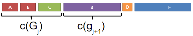
(b) Our constraint $c(g_{j+1})\leq c(G_{j})$ induces a smoother cost increase.

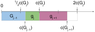
(c) Illustration of Doubling Algorithm Cost Constraint

Figure 1: Doubling Algorithm (b) has better anytime behaviors than greedy algorithm with no cost constraints (a).

1

input :  objective function $F$, elements $X$, minimum cost $c_{\textrm{min}}$

2

3Let $g_{1}=\underset{x\in X,\ c(x)\leq c_{\textrm{min}}}{\operatorname*{argmax}}\frac{F(\{x\})}{c(x)}$; Let $G_{1}=g_{1}$ ;

4 for $j=2,\ldots$ do

5       Let $g_{j}=\underset{x\in X\setminus G_{j-1},\ c(x)\leq c(G_{j-1})}{\operatorname*{argmax}}\;\frac{F(G_{j-1}\oplus\{x\})-F(G_{j-1})}{c(x)}$ ;

6       Let $G_{j}=G_{j-1}\oplus\{g_{j}\}$ ;

7      

Algorithm 2 Doubling Algorithm

Definition 4.2.

Let $G=(g_{1},\ldots)$ be the sequence selected by the doubling algorithm. The set $X$ and function $F$ are doubling capable if, at every iteration $j$, the following set is non-empty: $\{x\mid x\in X\setminus G_{j-1},\ c(x)\leq c(G_{j-1})\}$

Theorem 4.3.

Let $G=(g_{1},\ldots)$ be the sequence selected by the doubling algorithm (Algorithm 2). Fix some $B>c_{\textrm{min}}$. Let $F$ be $\gamma$-approximately submodular as in Definition 9. For any sequence $S$,

$$F(G_{\langle B\rangle})>\left(1-e^{-\frac{\gamma^{2}}{1+\gamma}}\right)F(S_{\langle\frac{B}{4}\rangle}).$$

Proof.

Doubling capable easily leads to the observation that for all budgets $B$, there exists an index $j$ such that $\frac{B}{2}\leq c(G_{j})<B$. Choose $K$ and $k$ to be the largest integers such that $\frac{B}{2}\leq c(G_{K})<B$ and $\frac{B}{8}\leq c(G_{k})<\frac{B}{4}$. Since at each step we at most double the total cost and $4c(G_{k})<B$, we observe $K\geq k+2$. For each $j$, define $s_{j}=\frac{F(G_{j+1})-F(G_{j})}{c(g_{j+1})}$ as the best rate of improvement among the items Doubling Algorithm is allowed to consider after choosing $G_{j}$. Consider the item $x$ in sequence $S_{\langle\frac{B}{4}\rangle}$ of the maximum cost.

(Case 1) If $c(x)\leq c(G_{k})$, then every item in $S_{\langle\frac{B}{4}\rangle}$ was a candidate for $g_{j}$ for all $j=k+1,...,K$. So by approximate submodularity from Equation 9, we have

$$F(S_{\langle\frac{B}{4}\rangle})\leq F(S_{\langle\frac{B}{4}\rangle}\cup G_{j})\leq F(G_{j})+\frac{Bs_{j}}{4\gamma}.$$ (12)

Then using the standard submodular maximization proof technique, we define $\Delta_{j}=F(S_{\langle\frac{B}{4}\rangle})-F(G_{j})$. Applying $s_{j}=\frac{\Delta_{j}-\Delta_{j+1}}{c(g_{j+1})}$ in the above inequality, we have $\Delta_{k+j}\leq\Delta_{k}\prod_{j=k+1}^{k+j}(1-\gamma\frac{4c(g_{j})}{B})$. Maximizing the inequality by setting $c(g_{j})=\frac{B}{K-k}\leq\frac{c(G_{K})-c(G_{k})}{4(K-k)}$, and using $(1-z/l)^{l}<e^{-z}$, we have $F(G_{K})>(1-e^{-\gamma})F(S_{\langle\frac{B}{4}\rangle}).$

From now on, we assume that $c(x)>c(G_{k})$ and consider two cases by comparing $c(g_{k+2})$ and $c(G_{k})$.

(Case 2.1) If $c(g_{k+2})\geq c(G_{k})$, then $c(G_{K})-c(G_{k+1})\geq c(g_{k+2})\geq c(G_{k})$. Since $c(G_{k+1})\leq 2c(G_{k})$ and $c(x)>c(G_{k})$, we have $c(G_{K})-c(G_{k+1})\geq\frac{B}{2}-2c(G_{k})$. So $c(G_{K})-c(G_{k+1})\geq\max(c(G_{k}),\frac{B}{2}-2c(G_{k}))\geq\frac{B}{6}$. Thus, using the same proof techniques as in case 1, we can analyze the ratio between $\Delta_{k+1}$ and $\Delta_{K}$, and have: $F(G_{K})>(1-e^{-\frac{2}{3}\gamma})F(S_{\langle\frac{B}{4}\rangle}).$

(Case 2.2) Finally, if $c(g_{k+2})<c(G_{k})<c(x)<c(G_{k+1})$, $g_{k+2}$ was a candidate for $g_{k+1}$, and $x$ was a candidate for $g_{k+2}$. For an item $y$, let $r(y^{j})=\frac{F(G_{j}\cup\{y\})-F(G_{j})}{c(y)}$ be the improvement rate of item $y$ at $G_{j}$. Then we have $r(g_{k+1}^{k})>r(g_{k+2}^{k})$ and $r(g_{k+2}^{k+1})>r(x^{k+1})$. Since the objective function is increasing, we have $r(x^{k})c(x)\leq r(x^{k+1})c(x)+r(g_{k+1}^{k})c(g_{k+1})$, so that $r(x^{k})\leq r(x^{k+1})+r(g_{k+1}^{k})\frac{c(g_{k+1})}{c(x)}$. Then by the definition of $\gamma$ in Equation 9, we have $\gamma r(g^{k+1}_{k+2})\leq r(g_{k+2}^{k})$. Hence we have $\gamma r(x^{k+1})\leq r(g_{k+1}^{k})$, which leads to $r(x^{k})\leq r(g_{k+1}^{k})(\frac{1}{\gamma}+\frac{c(g_{k+1})}{c(x)})\leq r(g_{k+1}^{k})(1+\frac{1}{\gamma})$. Then inequality (12) holds with a coefficient adjustment and becomes $F(S_{\langle\frac{B}{4}\rangle})\leq F(G_{k})+\frac{Bs_{k}(1+\gamma)}{4\gamma^{2}}.$ Noting that the above inequality holds for all $j=k+1,...,K$, we can replace the constant $\gamma$ in the proof of case $1$ with $\frac{\gamma^{2}}{1+\gamma}$ and have the following bound: $F(G_{K})>(1-e^{-\frac{\gamma^{2}}{1+\gamma}})F(S_{\langle\frac{B}{4}\rangle}).$

∎

5 EXPERIMENTS

Table 1: Test time 0.97-Timeliness measurement of different methods on Agricultural. We break the methods into OMP, FR and Oracle family: e.g., “Single” in the G-CS-OMP family means G-CS-OMP-Single, and “FR” in the Oracle family means the oracle curve derived from G-FR.

CS-G-OMP-Variants				CS-G-FR	Oracles		Sparse
CS-G-OMP	Single	No-Whiten	G-OMP		FR Oracle	OMP Oracle
0.4406	0.4086	0.4340	0.4073	0.4525	0.4551	0.4508	0.3997

Table 2: Test time 0.99-Timeliness measurement of different methods on Yahoo! LTR.

Group	CS-G-OMP-Variants				CS-G-FR	Oracles		Sparse
Size	CS-G-OMP	Single	No-Whiten	G-OMP		FR	OMP
5	0.3188	0.3039	0.3111	0.2985	0.3222	0.3225	0.3211	0.2934
10	0.3142	0.3117	0.3079	0.2909	0.3205	0.3207	0.3164	0.2858
15	0.3165	0.3159	0.3116	0.2892	0.3213	0.3213	0.3177	0.2952
20	0.3161	0.3124	0.3065	0.2875	0.3180	0.3180	0.3163	0.2895

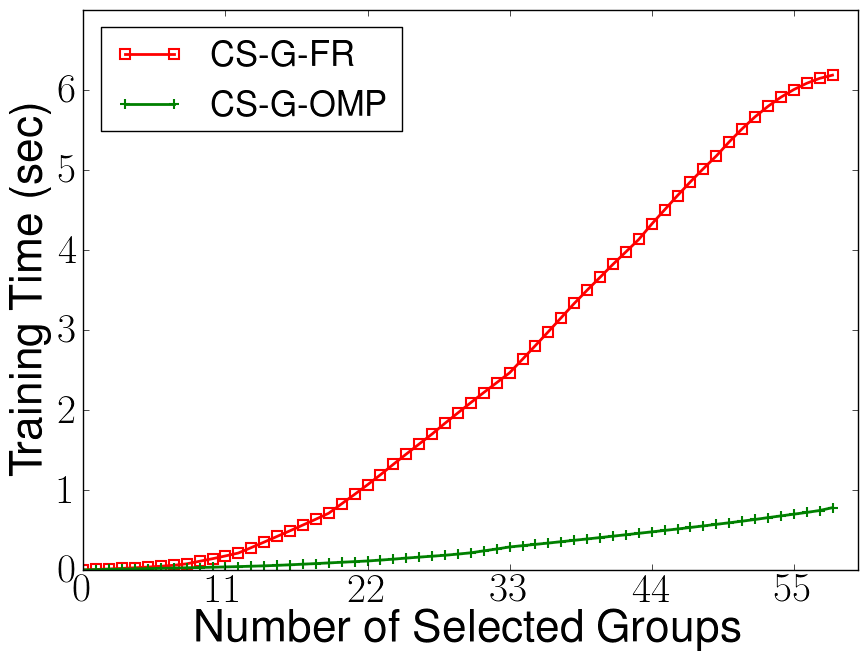
(a) Training Time OMP vs. FR (Agricultural)

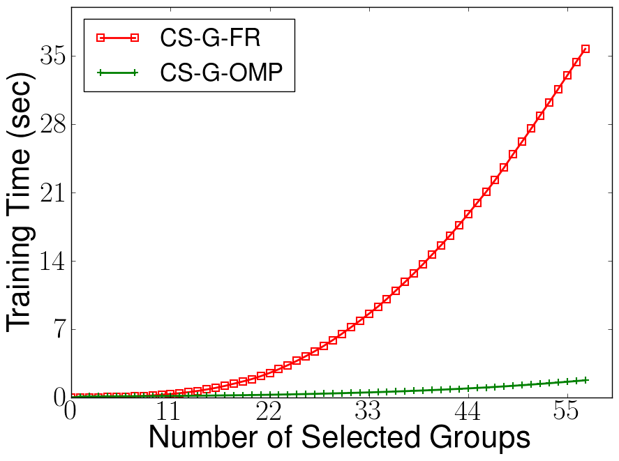
(b) Training Time OMP vs. FR (Yahoo! LTR)

Figure 2: The training time vs. the number of feature groups selected with two algorithms: CS-G-FR and CS-G-OMP. CS-G-OMP achieves a 8x and 20x overall training time speed-up on Agricultural  and Yahoo! LTR.

5.1 DATA-SETS AND SET-UP

We experiment our methods for anytime linear prediction on two real-world data-sets, each of which has a significant number of feature groups with associated costs.

• Yahoo! Learning to Rank Challenge (Chapelle and Chang, 2011) contains 883k web documents, each of which has a relevance score in $\{0,1,2,3,4\}$. Each of the 501 document features has an associated computational cost in $\{1,5,20,50,100,150,200\}$; the total feature cost is around 17K. The original data-set has no feature group structures, so we generated random group structures by grouping features of the same cost into groups of a given size $s$.

• Agriculture is a proprietary data-set that contains 510k data samples, 328 features, and 57 feature groups. Each sample has a binary label in $\{1,2\}$. Each feature group has an associated cost measured in its average computation time.

5.2 EVALUATION METRIC, BASELINE AND ORACLE

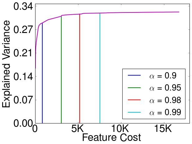
(a) Plateau Effect and $\alpha$-Stopping Costs

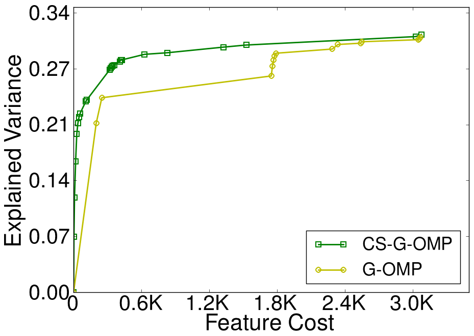
(b) Importance of Costs (CS-G-OMP vs. G-OMP)

Figure 3: (a) Explained Variance vs. Cost curve of CS-G-OMP in Yahoo! LTR. Vertical lines mark different $\alpha$-stopping costs. (b) Explained Variance vs. Cost curve of CS-G-OMP and G-OMP on Yahoo! LTR  set 1 with individual group size $s=10$, stopped at 0.97-stop cost.

Following the practice of Karayev et al. (2012), we use the area under the maximization objective $F$ (explained variance) vs. cost curve normalized by the total area as the timeliness measurement of the anytime performance of an algorithm. In our data-sets, the performance of linear predictors plateaus much before all features are used, e.g., Figure 3a demonstrates this effect in Yahoo! LTR, where the last one percent of total improvement is bought by half of the total feature cost. Hence the majority of the timeliness measurement is from the plateau performance of linear predictors. The difference between timeliness of different anytime algorithms diminishes due to the plateau effect. Furthermore, the difference vanishes as we include additional redundant high cost features. To account for this effect, we stop the curve when it reaches the plateau. We define an $\alpha$-stopping cost for parameter $\alpha$ in $[0,1]$ as the cost at which our CS-G-OMP achieves $\alpha$ of the final objective value in training and ignore the objective vs. cost curve after the $\alpha$-stopping cost. We call the timeliness measure on the shortened curve as $\alpha$-timeliness; 1-timeliness equals the normalized area under the full curve and 0-timeliness is zero. If a curve does not pick a group at $\alpha$-stopping cost, we linearly interpolate the objective value at the stopping cost to computr timeliness. We say an objective vs. cost curve has reached its final plateau if at least 95% of the total objective has been achieved and the next 1% requires more than 20% feature costs. (If the plateau does not exist, we use $\alpha=1$.) Following this rule, we choose $\alpha=0.97$ for Agricultural and $\alpha=0.99$ for Yahoo! LTR.

Since an exhaustive search for the best feature sequencing is intractable, we approximate with the Oracle anytime performance following the approach of Karayev et al. (2012). Given an objective vs. cost curve of a sequencing, we reorder the feature groups in descending order of their marginal benefit per unit cost, assuming that the marginal benefits stay the same after reordering. We specify which sequencing is used for creating Oracle in Section 5.5. For baseline performance, we use cost-weighted Group Lasso (Yuan and Lin, 2006), which scales the regularization constant of each group with the cost of the group. We note that the cascade design by Chen et al. (2012) can be reduced to this baseline if we enforce linear prediction. More specifically, the baseline solves the following minimization problem: $\min_{w\in\mathbb{R}^{D}}\|Y-Xw\|^{2}_{2}+\lambda\sum_{j=1}^{J}c(\mathcal{G}_{j})\|w_{\mathcal{G}_{j}}\|_{2},$ and we vary value of regularization constant $\lambda$ to obtain lasso paths. We call this baseline algorithm Sparse.

5.3 FEATURE COST

Our proposed CS-G-OMP differs from Group Orthogonal Matching Pursuit (G-OMP) (Lozano et al., 2009) in that G-OMP does not consider feature costs when evaluating features. We show that this difference is crucial for anytime linear prediction. In Figure 3b, we compare the objective vs. costs curves of CS-G-OMP and G-OMP that are stopped at 0.97-stopping cost on Yahoo! LTR. As expected, CS-G-OMP achieves a better overall prediction at every budget, qualitatively demonstrating the importance of incorporating feature costs. Table 1 and Table 2 quantify this effect, showing that CS-G-OMP achieves a better timeliness measure than regular G-OMP.

5.4 GROUP WHITENING

We provide experimental evidence that Group whitening, i.e., $X_{g}^{T}X_{g}=I_{D_{g}}$ for each group $g$, is a key assumption of both this work and previous feature group selection literature by Lozano et al. (2009, 2011). In Figure 4, we compare anytime prediction performances using group whitened data against those using the common normalization scheme where each feature dimension is individually normalized to have zero mean and unit variance. The objective vs. cost curve qualitatively shows that group whitening consistently results in the better predictions. This behavior is expected from data-sets whose feature groups contain correlated features, e.g., group whitening effectively prevents selection step $(*)$ from overestimating the predictive power of feature groups of repeated good features. Table 1 and Table 2 demonstrate quantitatively the consistent better timeliness performance of CS-G-OMP over that of CS-G-OMP-no-whiten.

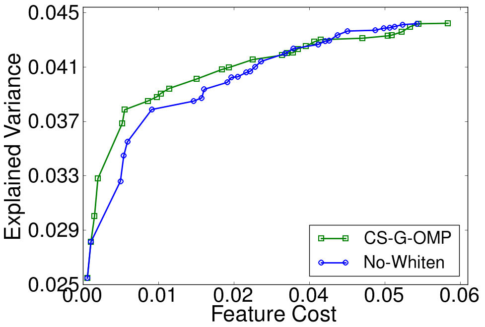
(a) Group Whiten vs. No-Whiten (Agricultural)

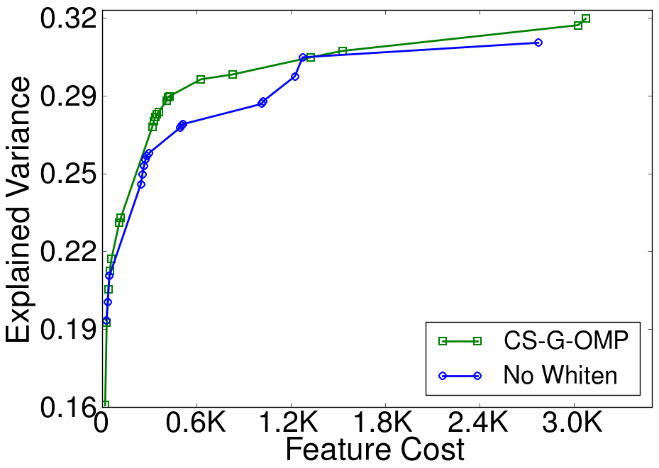
(b) Group Whiten vs. No-Whiten (Yahoo! LTR)

Figure 4: Explained Variance vs. Feature Cost curves on Agricultural  (a) and Yahoo! LTR  (b) comparing group whitening with no group whitening. The curves stop at 0.97-stopping cost.

5.5 SELECTION CRITERION VARIANTS

This section compares CS-G-OMP and CS-G-FR, along with variants of these two methods and the baseline, Sparse. We formulated the variant of CS-G-OMP, single, in Section 2 and it intuitively chooses feature groups of the best single feature dimension per group cost. Our experiments show that this modification degrades prediction performance of CS-G-OMP. Since FR directly optimizes the objective at each step, we expect CS-G-FR to perform the best and use its curve to compute the Oracle curve as an approximate to the best achievable performance.

In Figure 5, we evaluate CS-G-FR, CS-G-OMP and CS-G-OMP-single based on the objective in Theorem 3.2, i.e., explained variance vs. feature cost curves. CS-G-FR, as expected, outperforms all other methods. CS-G-OMP outperforms the baseline method, Sparse, and the CS-G-OMP-Single variant. The performance advantage of CS-G-OMP over CS-G-OMP-Single is much clearer in the Agricultural data-set than in the Yahoo! LTR data-set. Agricultural has a natural group structure which may contain correlated features in each group. Yahoo! LTR has a randomly generated group structure whose features were filtered by feature selection before the data-set was published (Chapelle and Chang, 2011). CS-G-FR and CS-G-OMP outperform the baseline algorithm, Sparse. We speculate that linearly scaling group regularization constants by group costs did not enforce Group-Lasso to choose the most cost-efficient features early. The test-time timeliness measures of each of the methods are recorded in Table 1 and Table 2, and quantitatively confirm the analysis above. Since Agricultural  and Yahoo! LTR  are originally a classification and a ranking data-set, respectively, we also report in Figure 5 the performance using classification accuracy and NDCG@5. This demonstrates the same qualitatively results as using explained variants.

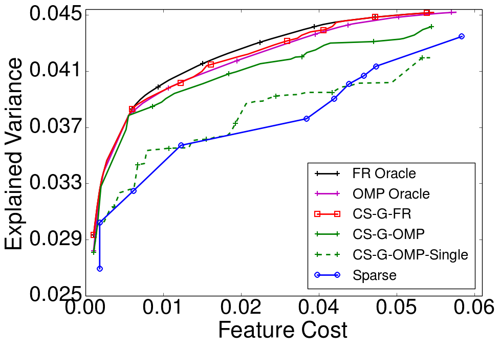
(a) FR vs. OMP vs. Sparse (Agricultural)

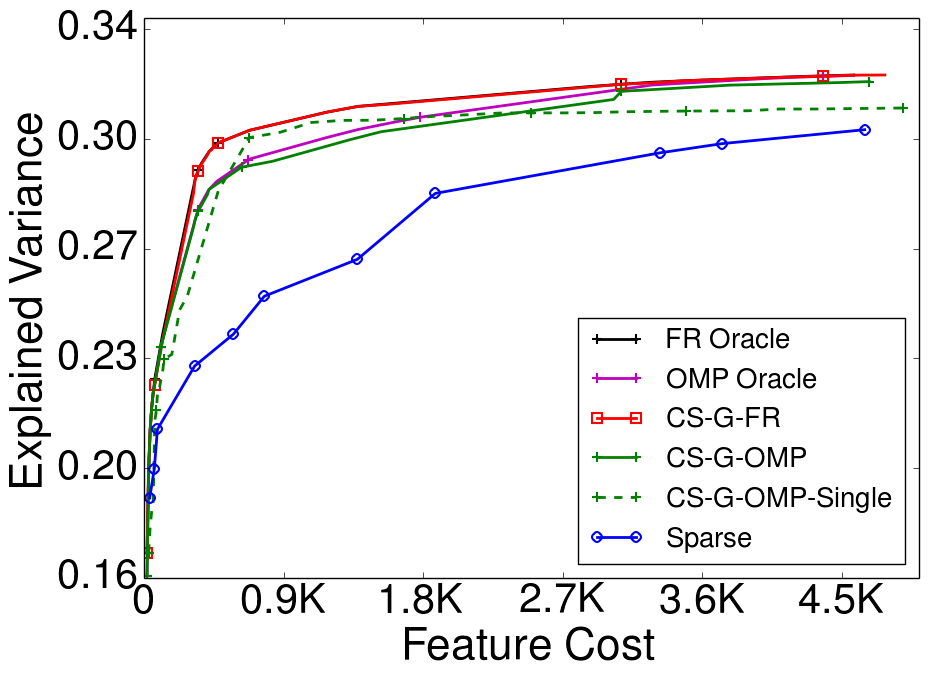
(b) FR vs. OMP vs. Sparse (Yahoo! LTR)

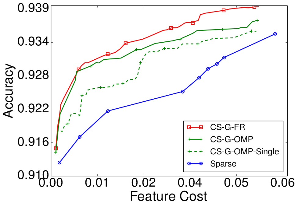
(c) FR vs. OMP vs. Sparse (Agricultural)

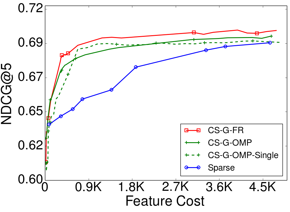
(d) FR vs. OMP vs. Sparse (Yahoo! LTR)

Figure 5: (a),(b): Explained Variance vs. Feature Cost curves on Agricultural  and Yahoo! LTR(group-size=10), using CS-G-OMP, CS-G-FR and their Single variants. Curves stop at 0.97 and 0.98 stopping costs. (c),(d): Same curve with the natural objectives of the data-sets: accuracy and NDCG@5.

As expected, when compared against CS-G-OMP, CS-G-FR consistently chooses more cost-efficient features at the cost of a longer training time. In the context of linear regression, let us assume that the group sizes are bounded by a constant when we are to select the number $K$ feature group. We can then compute a new model of $K$ groups in $O(K^{2}N)$ using Woodbury’s matrix inversion lemma, evaluate it in $O(KN)$, and compute the gradients with respect to the weights of unselected groups in $O(N(J-K))$. Thus, CS-G-OMP requires $O(K^{2}N+JN)$ at step $K=1,2,3,...,J$ and CS-G-FR requires $O((J-K)K^{2}N)$, so the total training complexities for CS-G-OMP and CS-G-FR are $O(J^{3}N)$ and $O(J^{4}N)$, using $\sum_{K=1}^{J}K^{2}=\frac{1}{6}J(J+1)(2J+1)$ and $\sum_{K=1}^{J}K^{3}=\frac{1}{4}J^{2}(J+1)^{2}$. We also show this training complexity gap empirically in Figure 2, which plots the curves of training time vs. number of feature groups selected. When all feature groups are selected, CS-G-OMP achieves a 8x speed-up in Agricultural over CS-G-FR. In Yahoo! LTR, CS-G-OMP achieves a speed-up factor between 10 and 20; the smaller the sizes of the groups, the larger speed-up due to the increase in the number of groups. Both greedy methods are much faster than the Lasso path computation using SPAMS, however.

Appendix A Additional Proof Details

This section describes a functional boosting view of selecting features for generalized linear models of one-dimensional response. We then prove Lemma 3.3 and Lemma 3.4 for this more general setting. These more general results in turn extend Theorem 3.2 to generalized linear models.

A.1 Functional Boosting View of Feature Selection

We view each feature $f$ as a function $h_{f}$ that maps sample $x$ to $x_{f}$. We define $f_{S}:\mathbb{R}^{D}\rightarrow\mathbb{R}$ to be the best linear predictor using features in $S$, i.e., $f_{S}(x)\triangleq w(S)^{T}x_{S}$. For each feature dimension $d\in D$, the coefficient of $d$ is in $w(S)$ is $w(S)_{d}=f_{S}(e_{d})$, where $e_{d}$ is the $d^{th}$ dimensional unit vector. So $\|w(S)\|_{2}^{2}=\sum_{d=1}^{D}\|f_{S}(e_{d})\|_{2}^{2}$. Given a generalized linear model with link function $\nabla\Phi$, the predictor is $E[y|x]=\nabla\Phi(w^{T}x)$ for some $w$ and the calibrated loss is $r(w)=\sum_{i=1}^{n}(\Phi(w^{T}x_{i})-y_{i}w^{T}x_{i})$. Replacing $f_{S}(x_{i})=w(S)^{T}x_{i}$, we have

$$r(w(S))=\sum_{i=1}^{n}(\Phi(f_{S}(x_{i}))-y_{i}f_{S}(x_{i})).$$ (13)

Note that the risk function in Equation 1 can be rewritten as the following to resemble Equation 13:

$$R(S)=\mathcal{R}[f_{S}]= \frac{1}{n}\sum_{i=1}^{n}(\Phi(f_{S}(x_{i}))-y_{i}^{T}f_{S}(x_{i}))$$

$${}+\frac{\lambda}{2}\sum_{d=1}^{D}\|f_{S}(e_{d})\|_{2}^{2}+A,$$ (14)

where $\phi(x)=\frac{1}{2}x^{2}$ for linear predictions and constant $A=\frac{1}{2n}\sum_{i=1}^{n}y_{i}^{2}$. Next we define the inner product between two functions $f,h:\mathbb{R}^{D}\rightarrow\mathbb{R}$ over the training set to be:

$$\langle f,h\rangle\triangleq\frac{1}{n}\sum_{i=1}^{n}f(x_{i})h(x_{i})+\frac{\lambda}{2}\sum_{d=1}^{D}f(e_{d})h(e_{d}).$$ (15)

With this definition of inner product, we can compute the derivative of $\mathcal{R}$:

$$\nabla\mathcal{R}[f]=\sum_{i=1}^{n}(\nabla\Phi(f(x_{i}))-y_{i})\delta_{x_{i}}+\sum_{d=1}^{D}f(e_{d})\delta_{e_{d}},$$ (16)

where $\nabla\phi(x)=x$ for linear predictions, and $\delta_{x}$ is an indicator function for $x$. Then the gradient of objective $F(S)$ w.r.t coefficient $w_{f}$ of a feature dimension $d$ can be written as:

$$b_{d}^{S} =-\frac{1}{n}\sum_{i=1}^{n}(\nabla\Phi_{p}(w(S)^{T}x^{i})-y^{i})x^{i}_{d}-\lambda w(S)_{d}$$ (17)

$$=-\langle\nabla\mathcal{R}[f_{S}],h_{d}\rangle.$$ (18)

In addition, the regularized covariance matrix of features $C$ satisfies,

$$C_{ij}=\frac{1}{n}X_{i}^{T}X_{j}+\lambda I(i=j)=\langle h_{i},h_{j}\rangle,$$ (19)

for all $i,j=1,2,...,D$. So in this functional boosting view, Algorithm 1 greedily chooses group $g$ that maximizes, with a slight abuse of notation of $\langle\;,\;\rangle$, $\|\langle h_{g},\nabla\mathcal{R}[f_{S}]\rangle\|_{2}^{2}/c(g)$, i.e., the ratio between similarity of a feature group and the functional gradient, measured in sum of square of inner products, and the cost of the group

A.2 Proof of Lemma 3.3 and Lemma 3.4

The more general version of Lemma 3.3 and Lemma 3.4 assumes that the objective functional $\mathcal{R}$ is $m$-strongly smooth and $M$-strongly convex using our proposed inner product rule. $M$-strong convexity is a reasonable assumption, because the regularization term $\|w\|_{2}^{2}=\sum_{d=1}^{D}\|f_{S}(e_{d})\|_{2}^{2}$ ensures that all loss functional $\mathcal{R}$ with a convex $\Phi$ strongly convex. In the linear prediction case, both $m$ and $M$ equals $1$.

The following two lemmas are the more general versions of Lemma 3.3 and Lemma 3.4.

Lemma A.1.

Let $\mathcal{R}$ be an m-strongly smooth functional with respect to our definition of inner products. Let $S$ and $G$ be some fixed sequences. Then

$$F(S)-F(G)\leq\frac{1}{2m}\langle b^{G}_{G\oplus S},C_{G\oplus S}^{-1}b^{G}_{G\oplus S}\rangle$$

Proof.

First we optimize over the weights in $S$.

$${}F(S)-F(G)$$

$$=\mathcal{R}[f_{G}]-\mathcal{R}[f_{S}]=\mathcal{R}[f_{G}]-\mathcal{R}[\sum_{s\in S}\alpha_{s}^{T}h_{s}]$$

$$\leq\mathcal{R}[f_{G}]-\min_{w:w_{i}^{T}\in\mathbb{R}^{d_{s_{i}}},s_{i}\in S}\mathcal{R}[\sum_{s_{i}\in S}w_{s_{i}}^{T}h_{s_{i}}]$$

Adding dimensions in $$G$$ will not increase the risk, we have:

$$\leq\mathcal{R}[f_{G}]-\min_{w:w_{i}\in\mathbb{R}^{d_{s_{i}}},s_{i}\in G\oplus S}\mathcal{R}[\sum_{s_{i}\in G\oplus S}w_{s_{i}}h_{s_{i}}]$$

Since $$f_{G}=\sum_{g_{i}\in G}\alpha_{i}h_{g_{i}}$$, we have:

$$\leq\mathcal{R}[f_{G}]-\min_{w}\mathcal{R}[f_{G}+\sum_{s_{i}\in G\oplus S}w_{i}^{T}h_{s_{i}}]$$

Expanding using strong smoothness around $$f_{G}$$, we have:

$$\leq\mathcal{R}[f_{G}]-\min_{w}(\mathcal{R}[f_{G}]+\langle\nabla\mathcal{R}[f_{G}],\sum_{s_{i}\in G\oplus S}w_{i}^{T}h_{s_{i}}\rangle$$

$$\quad+\frac{m}{2}\|\sum_{s_{i}\in G\oplus S}w_{i}^{T}h_{s_{i}}\|_{2}^{2})$$

$$=\max_{w}-\langle\nabla\mathcal{R}[f_{G}],\sum_{s_{i}\in G\oplus S}w_{i}^{T}h_{s_{i}}\rangle-\frac{m}{2}\|\sum_{s_{i}\in G\oplus S}w_{i}^{T}h_{s_{i}}\|_{2}^{2}$$

$$=\max_{w}\langle b^{G}_{G\oplus S},w\rangle-\frac{m}{2}\langle w,C_{G\oplus S}w\rangle$$

Solving $w$ directly we have:

$$F(S)-F(G)\leq\frac{1}{2m}\langle b^{G}_{G\oplus S},C_{G\oplus S}^{-1}b^{G}_{G\oplus S}\rangle$$

∎

Lemma A.2.

Let $\mathcal{R}$ be a M-strongly convex functional with respect to our definition of inner products. Then

$$F(G_{j})-F(G_{j-1})\geq\frac{1}{2M(1+\lambda)}\langle{b^{G_{j-1}}_{g_{j}}},b^{G_{j-1}}_{g_{j}}\rangle$$ (20)

Proof.

After the greedy algorithm chooses some group $g_{j}$ at step $j$, we form $f_{G_{j}}=\sum_{\alpha_{i}}\alpha_{i}^{T}h_{g_{i}}$, such that

$$\mathcal{R}[f_{G}]=\min_{\alpha_{i}\in\mathbb{R}^{d_{g_{i}}}}\mathcal{R}[\sum_{g_{i}\in G_{j}}\alpha_{i}^{T}h_{g_{i}}]\leq\min_{\beta\in\mathbb{R}^{d_{g_{j}}}}\mathcal{R}[f_{G_{j-1}}+\beta h_{g_{j}}]$$

Setting $\beta=\arg\min_{\beta\in\mathbb{R}^{d_{g_{j}}}}\mathcal{R}[f_{G_{j-1}}+\beta h_{g_{j}}]$, using the strongly convex condition at $f_{G_{j-1}}$, we have:

$${}F(G_{j})-F(G_{j-1})$$

$$=\mathcal{R}[f_{G_{j-1}}]-\mathcal{R}[f_{G_{j}}]\geq\mathcal{R}[f_{G_{j-1}}]-\mathcal{R}[f_{G_{j-1}}+\beta h_{g_{j}}]$$

$$\geq\mathcal{R}[f_{G_{j-1}}]-(\mathcal{R}[f_{G_{j-1}}]+\langle\nabla\mathcal{R}[f_{G_{j-1}}],\beta h_{g_{j}}\rangle$$

$$\quad+\frac{M}{2}\|\beta h_{g_{j}}\|_{2}^{2})$$

$$=-\langle\nabla\mathcal{R}[f_{G_{j-1}}],\beta h_{g_{j}}\rangle-\frac{M}{2}\|\beta h_{g_{j}}\|_{2}^{2}$$

$$=\langle{b^{{G_{j-1}}}_{g_{j}}},\beta\rangle-\frac{M}{2}\langle\beta,C_{g_{j}}\beta\rangle$$

$$\geq\frac{1}{2M}\langle b^{{G_{j-1}}}_{g_{j}},C_{g_{j}}^{-1}b^{{G_{j-1}}}_{g_{j}}\rangle$$

$$=\frac{1}{2M(1+\lambda)}\langle{b^{{G_{j-1}}}_{g_{j}}},b^{{G_{j-1}}}_{g_{j}}\rangle$$

The last equality holds because each group is whitened, so that $C_{g_{j}}=(1+\lambda)I$. ∎

Note that the $(1+\lambda)$ constant is a result of group whitening, without which the constant can be as large as $(D_{g_{j}}+\lambda)$ for the worst case where all the $D_{g_{j}}$ number of features are the same.

The proofs above for Lemma A.1 and A.2 are for one-dimensional output responses. They can be easily generalized to multi-dimensional responses by replacing 2-norms with Frobenius norms and vector inner-products with “Frobenius products”, i.e., the sum of the products of all elements.

A.3 Proof of Main Theorem

Given Lemma A.1 and Lemma A.2, the proof of Lemma 3.1 holds with the same analysis with a more general constant $\gamma=\frac{m\lambda_{min}(C)}{M(1+\lambda)}$. The following prove our main theorem 3.2.

Proof.

(of Theorem 3.2, given Lemma 3.1) Define $\Delta_{j}=F(S_{\langle K\rangle})-F(G_{j-1})$. Then we have $\Delta_{j}-\Delta_{j+1}=F(G_{j})-F(G_{j-1})$. By Lemma  3.1, we have:

$$\Delta_{j} =F(S_{\langle K\rangle})-F(G_{j-1})$$

$$\leq\frac{K}{\gamma}[\frac{F(G_{j})-F(G_{j-1})}{c(g_{j})}]=\frac{K}{\gamma}[\frac{\Delta_{j}-\Delta_{j+1}}{c(g_{j})}]$$

Rearranging we get $\Delta_{j+1}\leq\Delta_{j}(1-\frac{\gamma c(g_{j})}{K})$. Unroll we get:

$$\Delta_{L+1} \leq\Delta_{1}\prod_{j=1}^{L}(1-\frac{\gamma c(g_{j})}{K})\leq\Delta_{1}(\frac{1}{L}\sum_{j=1}^{L}(1-\frac{\gamma c(g_{j})}{K}))^{L}$$

$$=\Delta_{1}(1-\frac{B\gamma}{LK})^{L}<\Delta_{1}e^{-\gamma\frac{B}{K}}$$

By definition of $\Delta_{1}$ and $\Delta_{L+1}$, we have:

$$F(S_{\langle K\rangle})-F(G_{\langle B\rangle})<F(S_{\langle K\rangle})e^{-\gamma\frac{B}{K}}$$

The theorem follows and linear prediction is the special case that $m=M$. ∎

Appendix B Extension to Generalized Linear Model

While we only formulated the feature group sequencing problem in linear prediction setting previously, we can extend our algorithm for generalized linear models and multi-dimensional responses. In general, we assume that we have $P$ dimensional responses, and predictions are of the form $E[y|x]=\nabla\phi(Wx)$, for some known convex function $\phi:\mathbb{R}^{P}\rightarrow\mathbb{R}$, and an unknown coefficient $P\times D$ matrix, $W$. Thus, the generalized linear prediction problem is to minimize over coefficient matrix $W:P\times D$:

$$\textbf{r}(W)=\frac{1}{n}\sum_{i=1}^{n}(\phi(Wx^{i})-y_{i}^{T}Wx_{i})+\frac{\lambda}{2}\|W\|^{2}_{F},$$ (21)

where $\lambda$ is the regularization constant for Frobenius norm of the coefficient matrix. In particular, we have $\phi(x)=\frac{1}{2}x^{2}$ for linear prediction. The risk of a collection of features, $S$, is then $R(S)=\underset{W:\forall g\notin SW_{g}=\textbf{0}}{\min}\textbf{r}(W)$. To extend CS-G-OMP to feature sequencing in this general setting, we again, at each step, take gradient of the objective r w.r.t. $W$, and choose the feature group that has the largest ratio of group gradient Frobenius norm square to group cost. More specifically, after choosing groups in $G$, we have a best coefficient matrix restricted to G, $W(G)$. Then we compute the gradient w.r.t. $W$ at $W(G)$ (we keep the convention that unselected groups have zero coefficients) as:

$$\nabla\textbf{r}(W)=\frac{1}{n}\sum_{i=1}^{n}(\nabla\phi(Wx^{i})-y_{i})x_{i}^{T}+\lambda W;$$ (22)

we then evaluate $\|\textbf{r}(W)_{g}\|_{F}^{2}/c(g)$ for each feature group $g$, and add the maximizer to the selected groups to create new models. Algorithm 3 demonstrates the procedure.

Our theoretical result Theorem 3.2 can also be proven in this general setting. Proofs of Lemma 3.3 and 3.4) in appendix are readily for generalized linear models. Given these two lemmas, our proofs of Lemma 3.1 and Theorem 3.2 hold as they are.

1

input : The data matrix $\textbf{X}=[\textbf{f}_{1},...,\textbf{f}_{D}]\in\mathbb{R}^{n\times D}$, with group structures, such that for each group $g$, $\textbf{X}^{T}_{g}\textbf{X}_{g}=I_{D_{g}}$. The cost $c(g)$ of each group $g$. The response matrix $\textbf{Y}\in\{0,1\}^{n\times P}$. The link function $\nabla\Phi$. Regularization constant $\lambda$.

output :  A sequence $((G_{j},W_{j}))_{j}$, where $G_{j}=(g_{1},g_{2},...,g_{j})$ is the sequence of first $j$ selected feature groups, $g_{1},g_{2},...,g_{j}$, and $W_{j}:P\times D$ restricted to features in $G_{j}$ is the associated coefficient matrix.

2

3$G_{0}=\emptyset$; $W_{0}=\textbf{0}$;

4 for $j=1,2,...$ do

5       Compute $\textbf{r}^{\prime}=\nabla\textbf{r}(W_{j-1})$ with Eq. 22;

       // Selection step (*)

6       $g_{j}=\arg\max_{g}\|\textbf{r}^{\prime}_{g}\|_{F}^{2}/c(g)$;

       // Append selected group

7       $G_{j}=G_{j-1}\oplus(g_{j})$;

       // Solve for the best model with selected feature

8       Use a GLM algorithm to minimize Eq. 21 restricted to features in $G_{j}$

9       $W_{j}=\underset{W:\forall g\notin G_{j}W_{g}=\textbf{0}}{\arg\min}R(W)$;

10      

Algorithm 3 Cost Sensitive Group Orthogonal Matching Pursuit (G-OMP) for Generalized Linear Models

References

• Brubaker etΒ al. [2008] S.Β Brubaker, J.Β Wu, J.Β Sun, M.Β Mullin, and J.Β Rehg. On the Design of Cascades of Boosted Ensembles for Face Detection. International Journal of Computer Vision, pages 65–86, 2008.
• Cai etΒ al. [2015] Zhaowei Cai, MohammadΒ J. Saberian, and Nuno Vasconcelos. Learning Complexity-Aware Cascades for Deep Pedestrian Detection. In International Conference on Computer Vision, ICCV, 2015.
• Chapelle and Chang [2011] Olivier Chapelle and YiΒ Chang. Yahoo! Learning to Rank Challenge Overview. JMLR Workshop and Conference Proceedings, 2011.
• Chen etΒ al. [2012] Minmin Chen, KilianΒ Q. Weinberger, Olivier Chapelle, Dor Kedem, and Zhixiang Xu. Classifier Cascade for Minimizing Feature Evaluation Cost. In Proceedings of the 15th International Conference on Artificial Intelligence and Statistics (AISTATS), 2012.
• Das and Kempe [2011] Abhimanyu Das and David Kempe. Submodular meets Spectral: Greedy Algorithms for Subset Selection, Sparse Approximation and Dictionary Selection . In Proceedings of the 28th International Conference on Machine Learning (ICML), 2011.
• Grass and Zilberstein [1996] Joshua Grass and Shlomo Zilberstein. Anytime Algorithm Development Tools. SIGART Bulletin, 1996.
• Grubb and Bagnell [2012] Alexander Grubb and J.Β Andrew Bagnell. SpeedBoost: Anytime Prediction with Uniform Near-Optimality. In the 15th International Conference on Artificial Intelligence and Statistics (AISTATS), 2012.
• Jenatton etΒ al. [2010] Rodolphe Jenatton, Julien Mairal, Guillaume Obozinski, and FrancisΒ R. Bach. Proximal Methods for Sparse Hierarchical Dictionary Learning. In Proceedings of the 27th International Conference on Machine Learning (ICML), 2010.
• Karayev etΒ al. [2012] Sergey Karayev, Tobias Baumgartner, Mario Fritz, and Trevor Darrell. Timely Object Recognition. In Conference and Workshop on Neural Information Processing Systems (NIPS), 2012.
• Krause and Golovin [2012] Andreas Krause and Daniel Golovin. Submodular Function Maximization. In Tractability: Practical Approaches to Hard Problems, 2012.
• Lefakis and Fleuret [2010] Leonidas Lefakis and Francois Fleuret. Joint Cascade Optimization Using a Product of Boosted Classifiers. In Advances in Neural Information Processing Systems (NIPS). 2010.
• Lozano etΒ al. [2009] AurelieΒ C. Lozano, Grzegorz Swirszcz, and Naoki Abe. Grouped Orthogonal Matching Pursuit for Variable Selection and Prediction. In Neural Information Processing Systems (NIPS), 2009.
• Lozano etΒ al. [2011] AurelieΒ C. Lozano, Grzegorz Swirszcz, and Naoki Abe. Group Orthogonal Matching Pursuit for Logistic Regression. In Proceedings of the 14th International Conference on Artificial Intelligence and Statistics (AISTATS), volumeΒ 15, 2011.
• Miller [1984] AlanΒ J. Miller. Subset Selection in Regression. In Journal of the Royal Statistical Society. Series A (General), Vol. 147, No. 3, pp. 389-425, 1984.
• Pati etΒ al. [1993] Y.Β Pati, R.Β Rezaiifar, and P.Β Krishnaprasad. Orthogonal Matching Pursuit : recursive function approximation with application to wavelet decomposition. In Asilomar Conference on Signals, Systems and Computers, 1993.
• Reyzin [2011] Lev Reyzin. Boosting on a budget: Sampling for feature-efficient prediction. In the 28th International Conference on Machine Learning (ICML), 2011.
• Sochman and Matas [2005] J.Β Sochman and J.Β Matas. WaldBoost: Learning for Time Constrained Sequential Detection. In the 2005 IEEE Computer Society Conference on Computer Vision and Pattern Recognition (CVPR), 2005.
• Streeter and Golovin [2008] M.Β Streeter and D.Β Golovin. An Online Algorithm for Maximizing Submodular Functions. In Proceedings of the 22nd Annual Conference on Neural Information Processing Systems (NIPS), 2008.
• Tibshirani [1994] Robert Tibshirani. Regression Shrinkage and Selection Via the Lasso. Journal of the Royal Statistical Society, Series B, 58:267–288, 1994.
• Viola and Jones [2001] PaulΒ A. Viola and MichaelΒ J. Jones. Rapid Object Detection using a Boosted Cascade of Simple Features. In 2001 IEEE Computer Society Conference on Computer Vision and Pattern Recognition (CVPR), 2001.
• Weinberger etΒ al. [2009] K.Q. Weinberger, A.Β Dasgupta, J.Β Langford, A.Β Smola, and J.Β Attenberg. Feature Hashing for Large Scale Multitask Learning. In Proceedings of the 26th Annual International Conference on Machine Learning (ICML), 2009.
• Xu etΒ al. [2012] Z.Β Xu, K.Β Weinberger, and O.Β Chapelle. The Greedy Miser: Learning under Test-time Budgets. In Proceedings of the 28th International Conference on Machine Learning (ICML), 2012.
• Xu etΒ al. [2013] Z.Β Xu, M.Β Kusner, G.Β Huang, and K.Β Q. Weinberger. Anytime Representation Learning. In Proceedings of the 30th International Conference on Machine Learning (ICML), 2013.
• Xu etΒ al. [2014] Z.Β Xu, M.Β J. Kusner, K.Β Q. Weinberger, M.Β Chen, and O.Β Chapelle. Classifier cascades and trees for minimizing feature evaluation cost. Journal of Machine Learning Research, 15(1):2113–2144, 2014.
• Yuan and Lin [2006] Ming Yuan and YiΒ Lin. Model Selection and Estimation in Regression with Grouped Variables. Journal of the Royal Statistical Society, 2006.
• Zhang [2009] Tong Zhang. On the Consistency of Feature Selection using Greedy Least Squares Regression. Journal of Machine Learning Research, 10:555–568, 2009.