Jet substructure and probes of CP violation in Vh production
Abstract
We analyse the () vertex in a model independent way using production. To that end, we consider possible corrections to the Standard Model Higgs Lagrangian, in the form of higher dimensional operators which parametrise the effects of new physics. In our analysis, we pay special attention to linear observables that can be used to probe CP violation in the same. By considering the associated production of a Higgs boson with a vector boson ( or ), we use jet substructure methods to define angular observables which are sensitive to new physics effects, including an asymmetry which is linearly sensitive to the presence of CP odd effects. We demonstrate how to use these observables to place bounds on the presence of higher dimensional operators, and quantify these statements using a log likelihood analysis. Our approach allows one to probe separately the and vertices, involving arbitrary combinations of BSM operators, at the Large Hadron Collider.
1 Introduction
Both before and after the discovery of a new resonance at the Large Hadron Collider (LHC) Aad:2012tfa ; Chatrchyan:2012ufa , much attention has been focused on how to efficiently determine its spin and couplings Espinosa:2012ir ; Ellis:2012rx ; Ellis:2012hz ; Espinosa:2012vu ; Corbett:2012dm ; Espinosa:2012im ; Azatov:2012bz ; Montull:2012ik ; Klute:2012pu ; Azatov:2012ga ; Gao:2010qx ; Choi:2002jk ; Ellis:2012wg ; DeRujula:2010ys ; Odagiri:2002nd ; Buszello:2002uu ; Bredenstein:2006rh ; BhupalDev:2007is ; DeSanctis:2011yc ; Ellis:2012mj ; Boughezal:2012tz ; Stolarski:2012ps ; Ellis:2012xd ; Djouadi:2013yb ; Godbole:2013saa ; Ellis:2013ywa ; Godbole:2011hw ; Muhlleitner:2012jy ; Boos:2013mqa ; Sun:2013yra ; Einhorn:2013tja ; Anderson:2013afp ; Masso:2012eq ; Nhung:2013lpa ; Heinemeyer:2013tqa ; Delaunay:2013npa ; Delaunay:2013pja ; Maltoni:2013sma ; Belusca-Maito:2014dpa ; Gavela:2014vra ; Biekoetter:2014jwa . Deviations from Standard Model (SM) behaviour would signal the presence of new physics beyond the Standard Model (BSM), and there are significant motivations for expecting such deviations to be present at some level, not the least given that new physics is expected to explain or clarify the nature of electroweak symmetry breaking. There are two main approaches for addressing BSM corrections to the Higgs sector. The first is to postulate the existence of a specific theory, and analyse how the particle content leads to corrections to SM observables. This approach must necessarily be used for collider experiments whose energy exceeds the lowest energy scale associated with the new physics (e.g. a new particle mass). The second possibility is to use effective field theory techniques to write down possible corrections to the SM Lagrangian in the form of additional operators, which ultimately arise from integrating out the new degrees of freedom in a particular BSM model. One may systematically classify these operators according to their mass dimension, such that higher-dimensional ones are suppressed by increasing powers of the new physics scale. For a given mass dimension, there is a finite set of possible independent operators. By including all of these (in a chosen basis), one allows for the most general corrections to the SM. This approach has the benefit of being completely model-independent, but at the price of being applicable only for energy scales which are below the lowest new physics scale. This is a reasonable assumption to make, given that current studies (such as those referred to above) appear to show only small deviations, if any, from the Standard Model.
In this paper, we focus on the coupling of the Higgs to vector bosons
, . The operators relevant for these interactions have been
classified
in Buchmuller:1985jz ; Contino:2013kra ; Grzadkowski:2010es .
It is important to understand that bounds derived on the vertex, do not automatically translate to
bounds on the vertex. For example, as argued in ref. Delaunay:2013npa , violation of custodial symmetry can arise
naturally in new physics models. While higher dimension operators may be constrained from precision tests as well as Higgs rates Banerjee:2013apa ; Belusca-Maito:2014dpa ; Ellis:2014dva , the constraints depend on various assumptions. Unambiguous and definitive constraints
can only be determined by directly probing the nature of the and vertices separately.
In
order to determine whether or not the higher dimension operators are present in nature, one must
study various scattering processes that involve the and
vertices. The decay of the Higgs boson to boson pairs at the LHC
has been studied
in Choi:2002jk ; Gao:2010qx ; DeRujula:2010ys ; Desai:2011yj ; Stolarski:2012ps ; Bolognesi:2012mm ; Chen:2014ona ; Chatrchyan:2013iaa ; CMS-PAS-HIG-14-014 ; 2013arXiv1310.8361D ,
which focused on the fully leptonic decay channel. Combined with LHC
data, this disfavours the possibility that the recently discovered
boson is purely pseudoscalar at
significance ATLAS-CONF-2013-013 ; CMS-PAS-HIG-13-002 ; Chatrchyan:2012jja ; PhysRevLett.110.081803 ; PhysRevD.89.092007 .
The decay of the Higgs to boson pairs is more difficult in
principle, due to the limited kinematic resolution inherent in having
missing energy in the final state. This mode has been investigated
in Bredenstein:2006rh ; DeSanctis:2011yc ; Gao:2010qx ; Ellis:2012wg ; Abazov:2014doa ; CMS-PAS-HIG-14-012 . As
ref. Ellis:2012wg in particular makes clear, the kinematic cuts
used to select events in this case may overly diminish the signal for
BSM effects.
Another possibility is to study the production of the Higgs boson via
vector boson fusion, and angular observables exist for distinguishing
various BSM
scenarios Plehn:2001nj ; Hankele:2006ma ; Andersen:2010zx ; Andersen:2008gc . However,
a deficiency of this mode is that it is not possible to unambiguously
separate BSM contributions to the and
vertices. Furthermore, ref. Djouadi:2013yb argued that the
momentum dependence associated with an anomalous vertex can have
a dramatic effect on the rapidities of the quarks that emit the vector
bosons, and consequently of the acceptance of the event selection
cuts.
Given the above difficulties, the possibility has been explored of
using a future electron-positron collider, such as the proposed
International Linear Collider (ILC) or
equivalent Miller:2001bi ; Han:2000mi ; Biswal:2008tg ; Biswal:2009ar ; Dutta:2008bh . The
different BSM corrections have different CP properties, which manifest
themselves in different angular decay products of the Higgs and
associated particles. An collider can explore this in detail
using polarised beams. In addition, the partonic centre of mass energy
is known precisely in such a collider, and one may distinguish
different contributions to the vertices using the fact that they
lead to different power-like growths of associated Higgs production
cross-sections near threshold Miller:2001bi . However, it is
still not possible to unambiguously determine BSM corrections to the
and vertices separately at such a collider 111
It is not easy to study the anomalous WWh couplings via the process since there are large irreducible
backgrounds to this process and a high degree of beam polarization as well as measurements of the polarization of the final states are required. See ref. Biswal:2008tg for details.
.
Whilst this is possible at the LHeC (a proposed
facility) AbelleiraFernandez:2012cc ; Biswal:2012mp , it is clearly advantageous to use the
LHC itself to achieve this.
In this paper, we show that one can indeed distinguish the presence of
higher dimensional operators at the LHC, using the associated
production of a Higgs with a vector boson ( production), where the
Higgs boson decays to a pair of quarks. For many years, it was
thought to be impossible to analyse this mode, due to the presence of
large QCD backgrounds. This situation has changed due to the
development of jet substructure techniques, as pioneered
in Butterworth:2008iy . By requiring the Higgs boson to be
boosted, the quark pair from its decay will be approximately
collinear. One may then distinguish the boosted Higgs signal by
looking for a fat jet, containing two smaller subjets (modulo a
filtering procedure) each of which reconstructs the
mass. Subsequently, a number of approaches for utilising jet
substructure have been
developed Ellis:2009su ; Ellis:2009me ; Krohn:2009th ; Soper:2011cr ; Soper:2010xk ,
together with analytic
understanding Dasgupta:2013ihk ; Dasgupta:2013via and
applications in experimental
analyses ATLAS:2012am ; Aad:2012meb ; Aad:2013gja ; Chatrchyan:2013rla ; Aad:2012raa ; Aad:2012dpa ; ATLAS:2012dp ; ATLAS:2012ds ; Chatrchyan:2012ku ; Chatrchyan:2012cx ; Chatrchyan:2012ypy . As
the present authors already pointed out in Godbole:2013saa ,
reconstructing both the Higgs momentum and the associated vector boson
opens up the use of polarisation-related methods for production,
analogous to those used in the studies mentioned above: the
spin state of the associated vector boson is influenced by the
presence of higher dimensional operators in the Higgs sector, so that
angular observables involving the vector boson decay products can be
used to constrain BSM physics. Furthermore, this can be done
separately for the and channels, allowing one to
independently elucidate the nature of the and vertices.
The structure of our paper is as follows. Throughout the remainder of this introduction, we discuss the framework we are using for higher dimensional operators in more detail. In section 2, we describe the details of our simulations and the selection cuts. We also make a note of higher order effects in both and production and describe kinematic reconstruction issues. In section 2.6 we describe the increased sensitivity to non-SM couplings of the vertex, mentioned earlier. In section 3 we construct and describe various angular observables that are able to discriminate the different non-SM couplings of the vertex. In section 4 we construct likelihoods out of various observables and estimate the required luminosity for the TeV LHC to constrain the anomalous couplings. In section 5 we construct a CP-odd asymmetry that is linearly sensitive to the CP-odd coupling and hence to CP violating effects in the vertex. Finally in section 6 we summarize and conclude.
1.1 Higher Dimensional Operators
As already mentioned in the introduction, one may encapsulate the
structure of BSM physics in a model-independent way by adding higher
dimensional operators to the SM Lagrangian. One starts by classifying
all possible higher-dimensional operators that can serve as
corrections to the Standard Model Lagrangian and that are
gauge-invariant, an exercise which was first carried out
in Burges:1983zg ; Leung:1984ni ; Buchmuller:1985jz . There is a
single dimension five operator which, after electroweak symmetry
breaking, is responsible for neutrino masses and mixings. One is then
motivated to proceed to dimension six operators, of which there are
many - ref. Buchmuller:1985jz lists over a hundred. However,
not all of these are independent, as one may use equations of motion
to relate them. To this end, ref. Grzadkowski:2010es showed
that there are 59 independent
operators. Reference Contino:2013kra expressed these in a basis
more directly suited to Higgs boson physics, and also discussed how
the coefficients of these operators scale differently if electroweak
symmetry breaking is weakly or strongly coupled. Effective operators
for a hypothetical spin one or spin two Higgs boson have been
presented in Artoisenet:2013puc , which also discusses their
implementation in a computational framework inclusive of
next-to-leading order matrix element corrections and parton shower
effects. A pedagogical review of the literature may be found in
section 2 of ref. Alloul:2013naa .
Since our objective is to study the Lorentz structure of the vertex for massive gauge bosons, we will only concern ourselves with a subset of the operators. It is sufficient to consider the following three operators 222These correspond to the operators , and in ref. Heinemeyer:2013tqa .
Here is the scale of new physics and the multiplicative Wilson coefficients , and parametrize the relative strengths of these operators. Writing the coupling in the form , where () are the polarization vectors of the two gauge bosons, the vertices one obtains are
| (1) |
| (2) |
where we have introduced the rescaled parameters
| (3) |
| (4) |
and also rescaled the contribution by a factor
in each case, to allow for full generality (i.e. sensitivity to
rescalings of the Standard Model contribution).
Note that while the terms in the first two lines of each of
eqs. (1, 2) are CP–even, the terms
in the third lines are CP–odd. Terms which are not proportional to
may be generated within the SM at higher orders of
perturbation theory, although the resulting couplings are likely to be
very small. Significantly large values of these couplings would be a
signal for BSM physics.
One should note that, since we will always consider this vertex in
processes where the V bosons are connected to external fermions, the
terms and vanish due to current conservation and we will not
consider them any further. Note that the extra factors of in
(, ) as compared to (, ) signal violation of
custodial symmetry. These factors disappear when the corresponding
, and operators are of equal
strength.
The aim of this paper is to perform a detailed study of angular observables designed to distinguish the three contributions to each vertex: SM, BSM CP even, and BSM CP odd, building upon the preliminary study of Godbole:2013saa . In what follows we will present results in terms of the vertex parameters appearing in eqs. (1) and (2), rather than the coefficients of the higher dimensional operators directly, in order to be more general. The choice of operators is not unique, and different choices will result in different translations between the two sets of parameters (eqs. (3) and (4)). We discuss the details of our analysis framework in the following section.
2 Event Simulation and Selection
We consider production (), where the decays
leptonically, and the boson to a pair.
Further, we use jet substructure algorithm techniques to not just separate QCD backgrounds but use it to reconstruct the parton-parton CMS frame for production.
In this section we describe the tools and methods used for our
analysis, including the selection cuts utilised for both and
production. We simulate all processes using MadGraph5 Alwall:2011uj , having implemented the effective
Lagrangian in FeynRules Christensen:2008py ; Alloul:2013bka . The output is
interfaced with Pythia6 Sjostrand:2006za for showering
and hadronization. We use the ‘Z2Star’ tune for Pythia6,
including initial and final state radiation along with effects of
multiple interactions, and use the CTEQ6L1 parton distribution
functions Pumplin:2002vw . We use FastJet Cacciari:2011ma to cluster jets.
Note that cross-checks were carried out at the parton level using analytic expressions.
Our selection cuts for these signal processes are as follows.
2.1 production
For production we require:
-
1.
A fat jet of radius and transverse momentum . After applying the mass drop and filtering procedure of Butterworth:2008iy on this fat jet, we require no more than three sub-jets with , , and radius , where is the separation of the two hardest subjets, both of which must be -tagged. In addition, we also require that the invariant mass of this jet system reconstructs the Higgs mass in the range - GeV.
-
2.
Exactly 2 leptons (transverse momentum , pseudo-rapidity ) of same flavour and opposite charge, with invariant mass within of the mass . These should be isolated.
-
3.
The reconstructed has a , with azimuthal angle satisfying .
The first selection requirement listed above is used to reconstruct
the decaying Higgs. The requirement for a fat jet with large
transverse momentum means that we are looking at events with a highly
boosted Higgs. Note that by allowing for a third hard jet inside the
fat jet, the procedure allows for an extra jet other than the two
b-jets originating from the radiation of a gluon from the
b-quarks. The second requirement allows for reconstruction of the Z
boson, where the isolation criterion removes most of the
and QCD background. The third requirement ensures that the Higgs and
the Z boson lie in almost the same plane of production as is expected
for the signal.
Note that the above selection criteria are applied after simulating a detector response to be described in section 2.3.
After cuts, the only significant surviving background process is + jets. Cross-sections at Leading Order (LO) after cuts are shown in table 1. The branching ratios were taken from Ref. Dittmaier:2011ti . The cross-sections for backgrounds, the SM, the pure CP–odd operator and the two BSM CP–even operators and are shown, with all other couplings set to zero in each case. The values of the BSM couplings are chosen so as to reproduce the SM total cross-section, without any selection cuts. Note that in spite of this choice of couplings, the cross-sections after cuts for the BSM cases are much higher than the SM, implying a greater acceptance for the BSM cases. We will elaborate on this point later.
| Channel | V+jets | Single top | |||||
| 0.355 | 0.28 | 0.13 | 0.06 | 1.45 | 2.14 | 7.11 | |
| 0.12 | 0.23 | 0 | 0 | 0.48 | 0.73 | 2.22 |
2.2 production
For production we require the following:
-
1.
The Higgs reconstructed as above.
-
2.
Exactly one hard lepton (, ), isolated as above.
-
3.
Missing transverse momentum .
-
4.
The reconstructed has and azimuthal angle satisfying .
-
5.
No additional jet activity with , and rapidity (to suppress single and top pair production backgrounds).
The difference between and is that in the latter case only the transverse momentum of the W boson can be determined in the detector. However, it is possible to some extent to reconstruct the neutrino momentum as will be discussed in what follows. The LO cross-section for the signal and major backgrounds are detailed in table 1. Once again, the choice of couplings is such that the total cross-section (before any kinematic cuts) is identical to the SM total cross-section. As in the case of , we see that in this case also, the cross-section after cuts is larger for the BSM couplings, indicating a higher acceptance of the selection cuts to BSM physics. In the following we describe certain detector effects that we have considered in our analysis.
2.3 Detector effects
While a full detector simulation is beyond the scope of this study, it is still important to check whether the inefficiencies of a detector do not dilute the effects that are observable with exact reconstruction. To this end we use the Delphes 3 package deFavereau:2013fsa for a fast simulation of detector response. We set the parameters of the detector simulation tuned for the CMS detector, with some modifications:
-
•
The lepton isolation radius R is set to a reduced value of 0.3, to allow for isolation of leptons in high transverse momentum events where the leptons will be collimated.
-
•
We modify the jet reconstruction algorithm for the detection of a boosted Higgs as described above and set the b-tagging efficiency to be while the mis-tagging efficiency for c-jets is and for all other jets is .
We use the Delphes package since it has been shown to give good agreement with data deFavereau:2013fsa . However, we do not carry out any validation with experiment for our choice of parameters as this is beyond the scope of the discussion presented here.
2.4 Higher order effects
At LO and at NLO in QCD, production occurs through
quark-initiated processes. The NLO (QCD) correction to the LO order
process is given entirely by corrections to the Drell-Yan
process Han:1991ia ; Baer:1992vx ; Ohnemus:1992bd . The NLO process
produces extra QCD radiation in the initial state thus affecting
observables such as the transverse momentum of the final state
particles. It should be noted that such effects are large only near
the threshold of the transverse momentum cuts due to collinear and/or
soft initial state radiation Dittmaier:2012vm . In fact the use
of asymmetric transverse momentum cuts on the V-boson ( GeV)
and Higgs ( GeV) transverse momenta means that most of this
effect will be concentrated in the region ( GeV).
However, the contribution to the cross-section from this region of phase space is small and hence we neglect this effect.
The K-factor (ratio to the LO order cross-section) for NLO (QCD) is
about , see for example ref. Dittmaier:2012vm . In the special kinematic region of the boosted analysis
the K-factor for both and was found to be in
Ref. Butterworth:2008iy . For the background the
K-factor was found to be about the same while for the K
factor is higher and about . The other main background,
production, was found to have a K-factor . We
will use these values of the K-factor in our analysis of likelihoods in section 4.
Furthermore, we simulate the kinematics of an extra jet using the MLM matching procedure Hoche:2006ph with one additional jet for both signal and background. We have checked that our results do not vary significantly with the addition of this extra jet. For production, since we veto events with additional hard jets to remove backgrounds, the effect of extra radiation on the observables we consider is negligible.
2.5 Reconstructing the neutrino momentum
One must reconstruct the neutrino in production to determine our angular observables. We identify the neutrino transverse momentum with the missing transverse momentum . As explained previously, the missing transverse momentum is approximated by taking the negative vector sum of the transverse momentum of all particles that can be detected (GeV). In order to evaluate the full four momentum of the neutrino, we demand that the squared sum of the neutrino and lepton momenta be equal to the squared boson mass , and solve the resulting quadratic equation. Comparing with the “true” Monte-Carlo generated neutrino momentum, we find that choosing a given solution out of the two possible ones, reconstructs the true neutrino momentum of the time, with giving imaginary solutions. One may improve on this by comparing the boosts of the Higgs and reconstructed in the direction. The solution with the minimum value for gives the true neutrino momentum in of cases. We thus present all our results using the latter algorithm.
2.6 Sensitivity to anomalous couplings
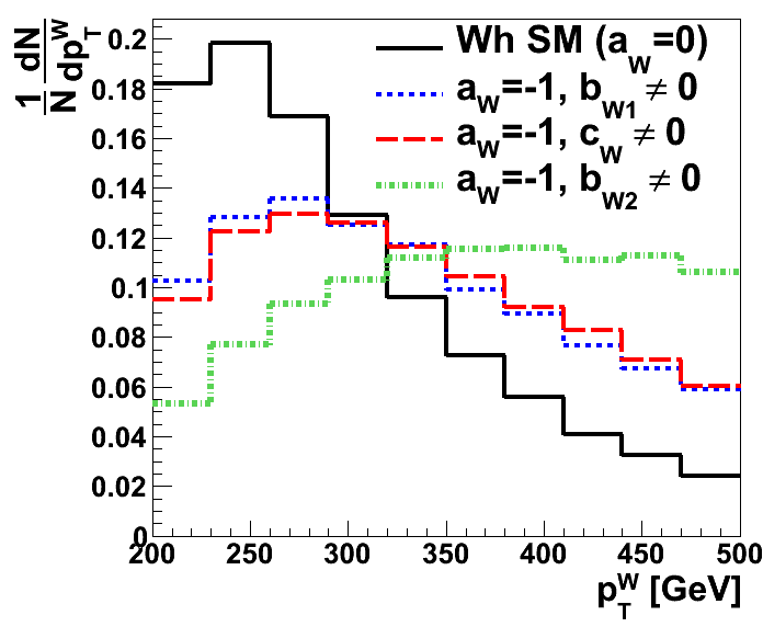
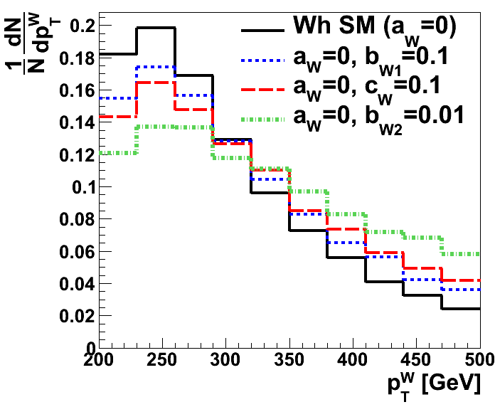
It has been observed that the momentum dependence of the BSM couplings
of the vertex push the and invariant mass
distributions to larger
values Djouadi:2013yb ; Ellis:2012xd ; Englert:2012ct , due
ultimately to the extra momentum factors present in the BSM
vertices. This is confirmed in the distributions shown in the plots in
figure 1. The plot on the left shows the transverse momentum
distribution of the boson in production in the SM (black
solid line) compared each of the pure BSM couplings (with the SM
contribution set to zero), using the selection cuts described in the
previous section. The values of the couplings have been chosen so that
they reproduce the SM cross-section when no cuts are applied. We see
that the effect of all the BSM couplings is to push the
distribution to larger values. The effect is even more pronounced for
the coupling while the and couplings have a strong
but less pronounced effect on this distribution. In the right plot we
show the same distribution but this time for admixtures of the SM
coupling () with each of the BSM couplings. The effect of the
BSM couplings is still easily discernible, though less prominent than
compared to the plot on the left. The larger distributions of the
system also lead to larger Higgs boosts and a reduced separation
and between the leptons (from the decay of the gauge
bosons) and jets (from the decay of the Higgs) respectively. As
mentioned in the previous section, this effect is further quantified
by the results of table 1, in which the cross-section for
pure BSM processes after cuts is significantly higher than the SM
result, after imposing that the cross-sections agree before cuts.
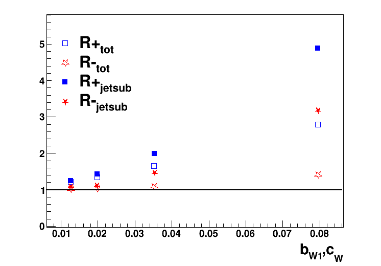
In figure 2, we consider the SM coupling supplemented by either the (CP–odd) coupling or the coupling applied to the channel. We show the ratio of the SM+BSM and SM cross-sections both for the total cross-section and the cross-section after applying selection cuts . Here and correspond to the case () and () respectively. As is expected, both ratios decrease with the strength of the BSM couplings and approach unity as the BSM couplings tend to zero. shows a faster rise with coupling strength than . This is because the interference term in the matrix element squared for the CP–odd coupling does not contribute to the cross-section333In practice, if the squared term is larger than the interference term, this is an indication that the effective theory framework is breaking down. Here, however, we are merely quantifying the effect by which selection cuts enhance BSM effects, by fixing the BSM cross-section to be artificially high (equivalent to an unphysically low cut-off scale).. Importantly, (for both couplings) increases at a faster rate than with increasing values of the corresponding couplings. Similar results also hold for the second CP–even anomalous coupling . These ratios are therefore quite sensitive to the presence of anomalous couplings. Whilst not directly experimentally measurable, they can be determined by comparing an experimental measurement of the signal with a precise theoretical prediction for the SM only contribution. If this lies away from unity, this constitutes a strong indication of BSM physics. Another feature that should be noted is that the ratio of the ratios () increases at a faster rate for the CP–odd coupling than it does for the CP–even coupling. This is in agreement with the results of table 1, where it was observed that the acceptance to the selection cuts of the pseudo-scalar state was higher than a scalar with anomalous coupling .
3 Angular observables
In this section, we consider differential observables that can
distinguish between the different BSM vertices occurring in the
interaction. One such observable, the transverse mass of the
system, has been used at the Tevatron to probe the
vertex Johnson:2013zza , however, it has been shown to be
ineffective at the LHC Ellis:2012xd . Furthermore, the CP-odd
coupling contributes to this observable only through quadratic terms
in the matrix element squared and therefore is not the most sensitive
observable 444Care must be taken if such quadratic terms become
important, as this signals a potential breakdown of the effective
theory description.. Angular observables, as we will show, can be
linearly sensitive to the anomalous couplings. This is useful in that
one may construct asymmetry parameters that are manifestly zero for
the SM, such that any non-zero measurement constitutes discovery of
new physics. Note that in the context of effective theory analysis, constructing
observables that are linear in the anomalous couplings is of paramount importance.
The tensor structure of the BSM vertices will be reflected in the angular distribution of the decay products of the gauge boson555Note, the Higgs has spin zero; angular distributions of its decay products are uncorrelated from production and hence do not carry any information about the vertex in production. Angular correlations of the decay products of the Higgs would reflect the properties of the decay vertex and not the production vertex; as in decays.. To this end, we construct various angular observables that could discriminate between the different vertex structures. The momenta of the and Higgs bosons are reconstructed from the leptons and jets as follows:
| (5) |
where are the momenta of the jets, is the momentum of the third jet if it is reconstructed and and are the momenta of the lepton and the anti-lepton respectively (for , corresponds to the lepton momentum and to the neutrino). With these momenta, we may define
| (6) |
Here corresponds to the three momentum of the
particle in the rest frame of the particle . If is not
specified then the momentum is defined in the lab frame. The
parameter corresponds to the angle between the
direction of the decaying lepton in the rest frame of the V boson with
the direction of flight of the V boson in the lab frame. This angle,
first defined in Miller:2001bi , encodes the boson
polarization.
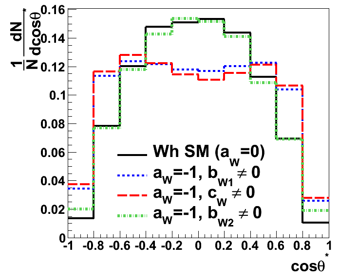
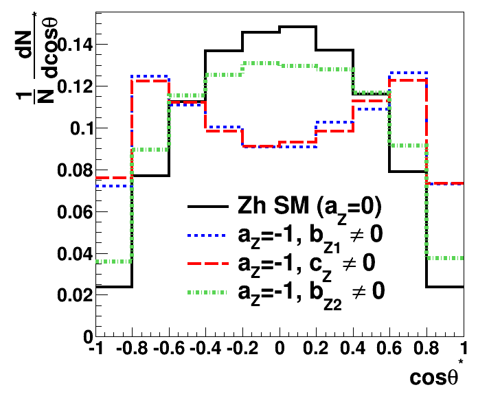
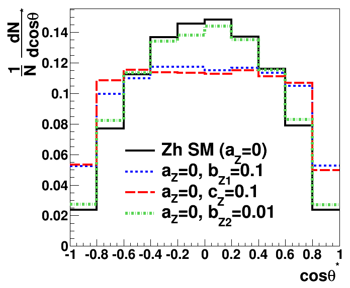
The SM and BSM couplings lead to mostly longitudinal and transverse
bosons respectively. That then effectively
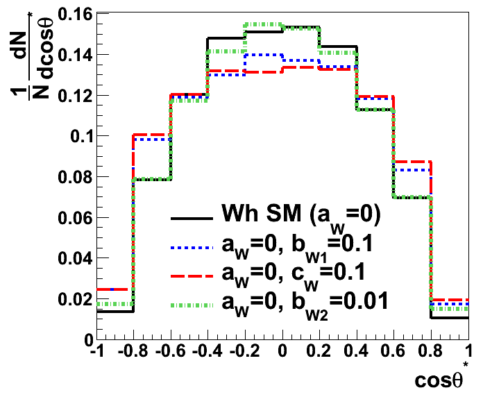
distinguishes SM and BSM effects can be seen in figure 3.
We see that the SM distribution (black solid line) peaks at
and vanishes at . The
distribution for the BSM coupling (green dot-dashed line)
closely follows the SM distribution. This is expected since the tensor
structure of the vertex in both these cases is the same. In contrast,
the couplings and produce distributions that have minima
at . They too appear to vanish at
, however this is the effect of the selection
cuts666All the selection cuts deplete this region of phase space, with strongest effects coming from the transverse momentum and rapidity cuts of the lepton.. Without applying any selection cuts the distribution for these
two cases peak at .
The behaviour of this distribution for each of the couplings can be
understood as follows. For a transversely polarized W boson, the
decay lepton spins align themselves perpendicular to the direction
of motion of the W boson and gives rise to a distribution of the form
, while in the case of a longitudinally
polarized W boson, the spins of the decay leptons align themselves
along the direction of the W boson and give rise to a distribution
of the form . The two BSM couplings and
produce more transversely polarized W boson states while the SM
coupling and the coupling produce more longitudinally polarized
W bosons. Using this distribution, it is therefore possible to
differentiate between vertex structures with couplings or
from the vertex structure with couplings or , but not
between and or between and .
In figure 4 we present plots of the same observable
for admixtures of the SM coupling with each of the
BSM couplings. We present three cases corresponding to
(), () and (). We see
that differences, though reduced, are still discernible in this
distribution. Similar results also hold for production.
To fully distinguish the CP even () and odd () BSM
contributions, one must construct CP-odd observables, which is
difficult in principle for a proton–proton
collider Han:2009ra . For production,
Ref. Christensen:2010pf considered two such observables,
although these are sensitive to radiation and hadronization
corrections; Ref. Englert:2012xt defined observables which are
insensitive to the CP nature of BSM contributions.
Ref. Desai:2011yj examined CP–odd asymmetries in
production with the decay , though the effect of
the BSM CP even term was not considered. The hint for possible CP–odd
observables comes from looking at the matrix element squared for the
process shown in appendix A. The
interference term between the CP–odd coupling and the SM coupling
(), is proportional to
, where and is
the anti-symmetric Levi-Civita tensor. Such a term depends on the
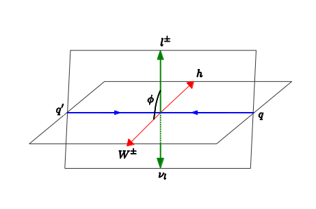
angle between the plane of production of the and the direction of
flight of the lepton. This is depicted in figure 5.
We now construct the following angles based on the observation made above.
| (8) |
We use the same notation for the momenta as described below eq. (6). For an collider where the direction (as well as the energy) of the lepton and anti-lepton are well known, it is sufficient to define the normal to the plane of production with the cross-product between any one of the leptons and the direction of flight of the Higgs or gauge boson. Note that the choice of vectors in collisions completely fixes whether the normal points ‘below’ or ‘above’ the plane of production. At the LHC, the information about the direction of the quark or anti-quark is not known and hence it is difficult to fix the direction of the normal to the plane of production. However, it is known that the valence quarks are likely to carry a larger fraction of the proton momentum. The direction of the normal to the plane of production can then be fixed by the momenta of the V and Higgs bosons.
We use this fact to construct the first angle in eq. (8),
, which corresponds to the angle between the direction
of flight of the lepton (with the momentum evaluated in the rest frame
of the V boson) and the plane formed by the V boson and the Higgs. In
an collider, where the centre-of-mass and lab frames
coincide, the gauge and Higgs bosons will be produced back to back.
However, at the LHC one can take advantage of the asymmetric collision
energies of the partons which results in the difference between the
centre-of-mass and lab frame. For asymmetric collisions, the plane
defined by the cross-product between the V boson and Higgs directions,
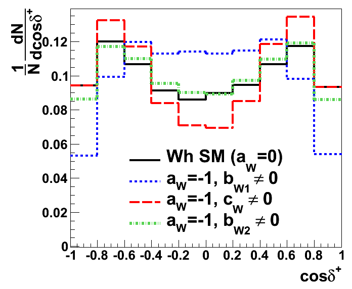
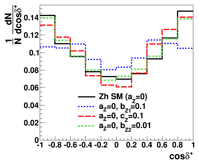
coincides with the plane of production. In figure 6 we show
the distribution of this observable for SM as well as for the
anomalous couplings. In the plot on the left, the SM prediction is
compared to the prediction for each of the anomalous couplings : (blue dotted line), (green dot-dashed) and (red
dashed) with all other couplings set to zero in each case. All
distributions show a dip at . This is created by the
transverse momentum cut on the leptons, since low leptons will
always be perpendicular to the normal to the plane of production.
We see from this distribution that for leptons are
produced mostly in the plane of production, while for the
leptons tend to be produced mostly perpendicular to the plane of
production. For two cases, the SM and for , the
distribution is flat (without cuts) and has a slight dip at
due to the cuts, as explained above. This
observable clearly discriminates between the and cases, a feature that was absent in the distributions of
observables discussed earlier.
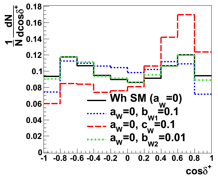
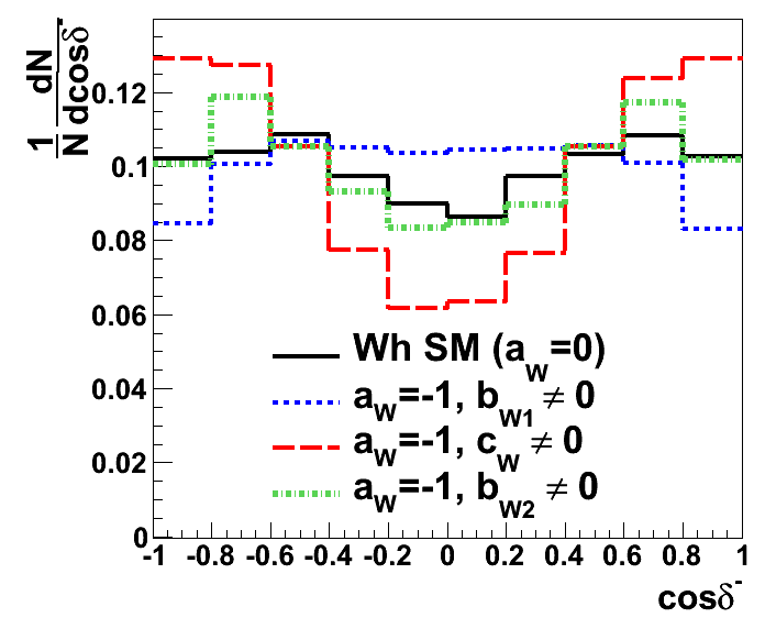
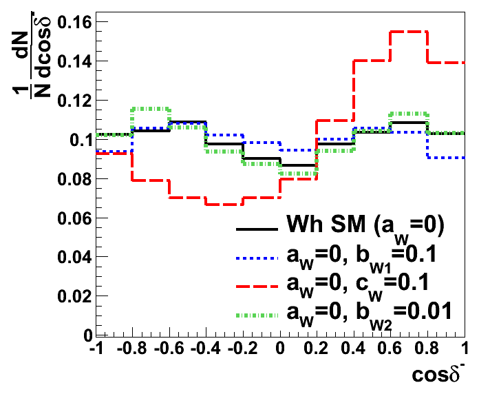
More interesting effects can be seen in this observable when we
consider admixtures of each of the anomalous couplings with the SM. In
the right plot of figure 6 the distribution of three cases
are compared with the SM expectation: (blue dotted
line), () (green dot-dashed) and
(red dashed), with all other couplings set to zero in each case. As
expected, the distribution for the case () follows
the SM distribution closely. The CP–even case is
similar to the pure anomalous coupling case ( ). We
have checked that the interference term alone for the case
produces a similar distribution to the case
() and is therefore linearly sensitive to . For the
CP violating case the distribution is skewed towards
positive values of . This is due to the presence of
the Levi-Civita tensor in the interference term of the matrix element
squared as described above. Note that the distribution will peak for
negative values of if the sign of the coupling
were changed. This observable is therefore, linearly sensitive
to and hence to its sign. We will use this fact to construct
asymmetries in the next section.
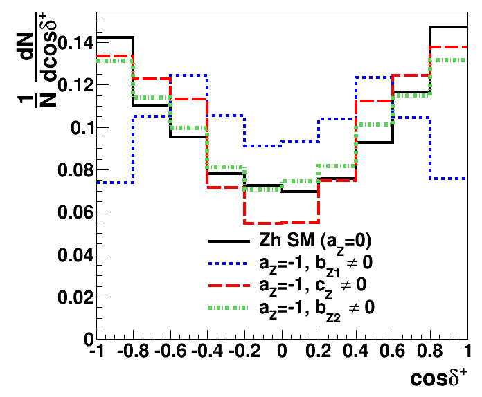
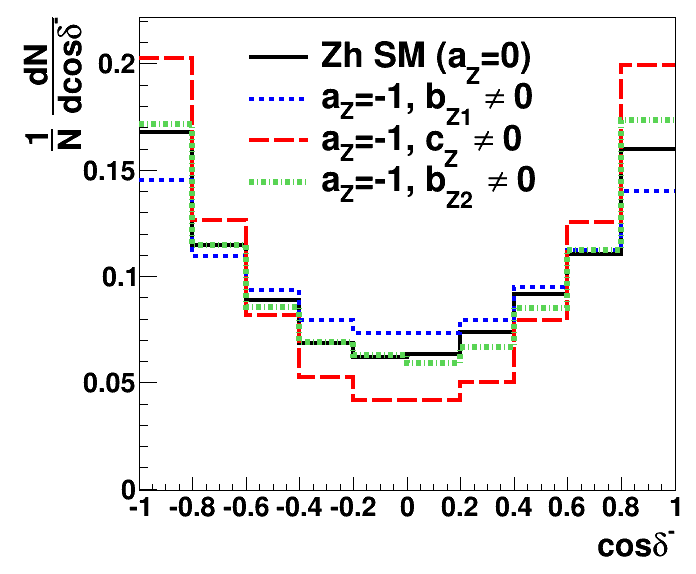
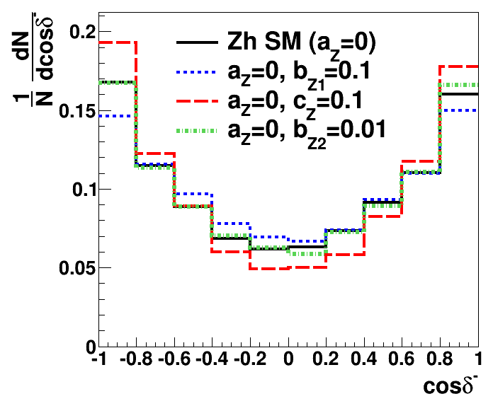
The second observable we consider is slightly more complicated in
construction. The momenta of the two leptons from the decay of the
gauge boson are evaluated in the frame in which the Higgs would be at
rest, were its three momentum reversed777If the four momentum
of the Higgs is written as , then this is the frame
defined by the boost such that . Then
is the angle between the plane formed by the two
leptons in this frame and the V boson in the lab frame. This angle is
related to the angle depicted in figure 5. The
distribution of this observable for SM is compared with three other
cases in the left plot of figure 7 : (blue
dotted line), (green dot-dashed) and (red
dashed) with all other couplings set to zero in each case. The right
plot of figure 7 compares the distribution of the SM
expectation with admixtures of the SM couplings and the BSM coupling
as given in the figure (and other couplings set to zero). The
behaviour of this angle is very similar to that of
. There are two noticeable differences. Firstly in the
case the distribution of appears to show
a more heightened difference from SM as compared to the distribution
for . For the case when the opposite is
true and appears to show a greater difference from
the SM distribution. This is also true when we set . For
the CP-violating case, the same skewed behaviour of the distribution
that was observed for , reappears here. As usual the
distribution for the coupling in both the pure and mixed cases
of the left and right plots of figure 7, follow closely the
SM expectation.
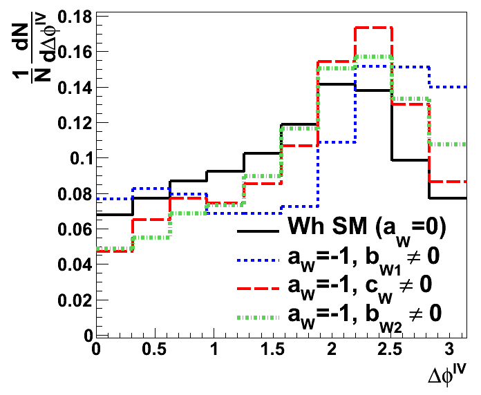
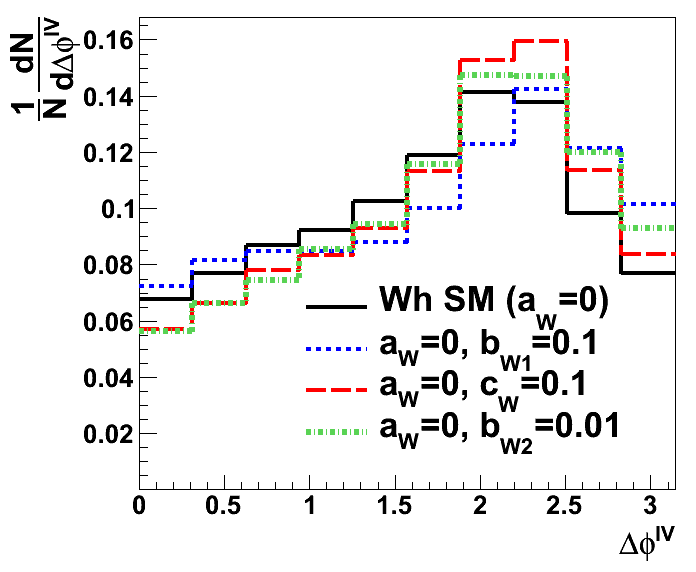
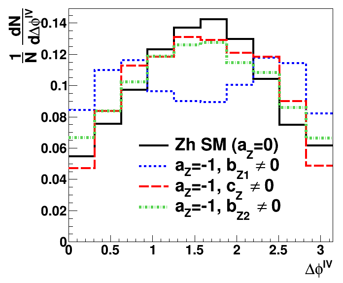
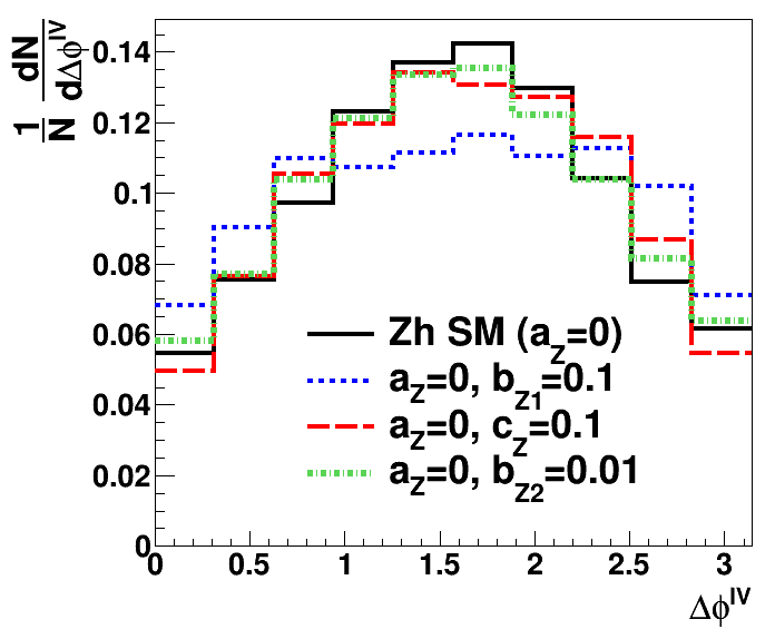
The last observable we consider () is the azimuthal
angle difference of the lepton momenta (evaluated in the rest frame of
the V boson) and the V boson momentum. The distribution for this
observable is shown in figure 8. The left plot compares the
SM expectation with three cases of the pure BSM couplings. The right
plot compares the SM prediction with admixtures of SM with each of the
BSM couplings. For all the cases we consider, there is a significant
difference from the SM distribution of this observable. The most
striking difference, however, is for the pure CP–even case () which displays a minimum in this distribution at
unlike the other cases. Differences between the distributions remain,
although reduced, when considering admixtures of the SM coupling
() with each of the BSM couplings.
We also show in figure 9 distributions of the observables described above for the backgrounds to production listed in table 1. The distribution of the various angles follow the SM distribution except for the angles and .
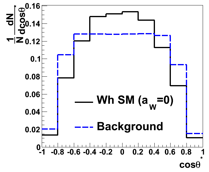
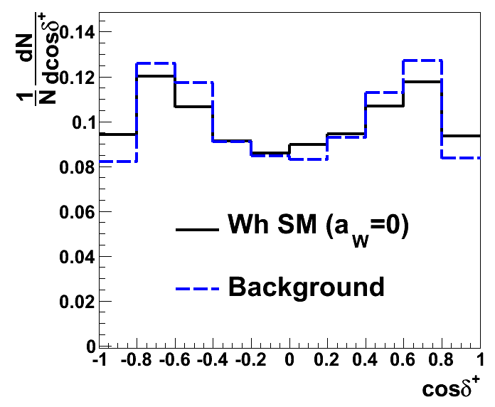
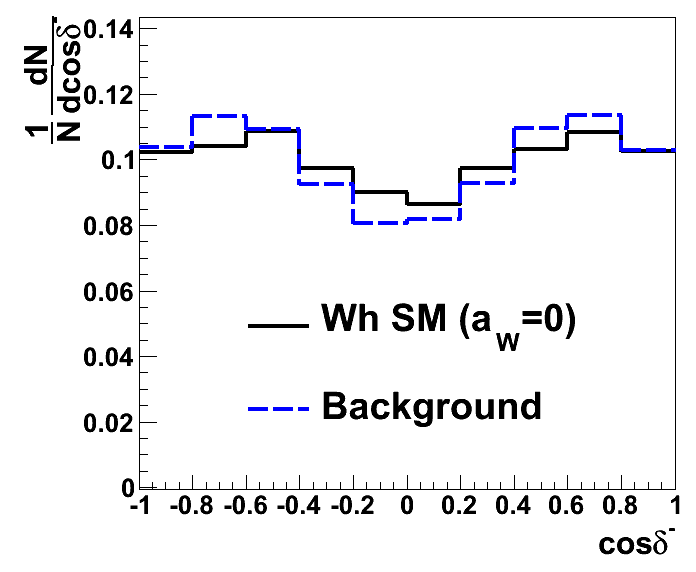
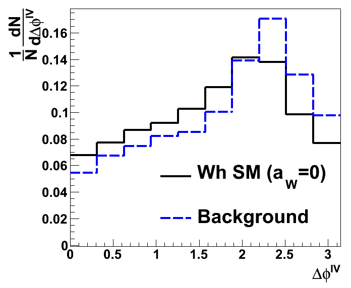
For completeness, we also show the distributions of the various angles
defined in eq. (6) and eq. (8) for
production. In figure 10, the SM distribution (black solid
line) is compared with the predictions of the three different BSM
couplings. The values of the couplings are chosen as in table 1,
so as to reproduce the SM total cross-section (before cuts). The
distributions display a similar behaviour as compared to the analogous
distributions in production.
In figure 11, the SM distribution (black solid line) is
compared with three cases which involve admixtures of the SM and BSM
couplings The asymmetries in the distributions of and
that one observes in production for the
CP-violating case , although present, are far less
prominent in production. The reason for this difference can be
ascertained by looking at the CP violating term in the matrix element
squared. For production, as described earlier, this term was
simply proportional to a Levi-Civita tensor of the form
. The CP violating term in the matrix element squared
for production has several instances of the Levi-Civita tensor
that come with opposite signs. These do not cancel out (as they do in
production) since they are multiplied by axial and vector
couplings (which are of different strengths). As a result, the
distributions of and receive
contributions from Levi-Civita tensors of opposite sign and hence
display a reduced skewness in distribution in comparison to the
analogous distribution in production.
We now have a set of observables that can discriminate not only the SM coupling from BSM couplings but also between the various BSM couplings, as evidenced by the distributions presented in this section. In order to fully assess the discriminating power of these observables and to estimate the typical luminosities that one would require at a TeV LHC to rule out the various anomalous couplings, we perform a multi-variable likelihood analysis in the next section.
4 Multi-Variable Likelihood analysis
In the previous section we described the various observables that one
could use in order to probe anomalous couplings in production. We
found that the transverse momentum of the V boson (or the Higgs), the
angle and any one of the correlated observables
defined in eq. (8) can be used for this purpose. It is
well known that the maximized log likelihood ratio provides the
strongest test statistic according to the Neyman-Pearson
lemma. Therefore in order to assess the sensitivity of these
observables to probe anomalous couplings at the LHC, we perform a
three dimensional extended binned-likelihood analysis. The procedure
we follow is outlined below.
We set the SM expectation () plus backgrounds as our null hypothesis. The alternate hypotheses are chosen to be the various cases which involve any one of the BSM couplings along with backgrounds. We define our likelihood as functions of a set of three observables. These are , and any one of the observables defined in eq. (8). In fact, we perform this analysis for three different definitions of the likelihood (L) which depend on the choice of observable, namely , and . As a first step we produce three dimensional histograms with the various combination of observables listed above. The choice of range and bins for each of the observables is listed below.
-
•
: range GeV, 10 bins
-
•
: range , 10 bins
-
•
: range , 10 bins
-
•
: range , 10 bins
The histograms are binned with at least events after applying
all selection cuts.
Using these histograms we can now determine the Likelihood function. Let be the expected bin height (or number of events) of the bin derived from theory (in our case from Monte Carlo simulations). The probability that the bin will have observed events (observed bin height) is a Poissonian probability given by
| (9) |
We can now proceed to determine the probability of generating the full distribution for all of the histogram bins by multiplying the probability for each of the bins. The binned likelihood is then given by a Poisson distribution
| (10) |
Here is the number of bins, is the expected number of events under the hypothesis and is the number of observed events. The likelihood ratio is then defined as
| (11) |
We now use these three dimensional histograms to generate
“pseudo-data”. This is done by using the theoretically determined
to generate Poisson distributed random numbers which correspond
to our pseudo-data. We repeat this procedure for all bins in order to
generate pseudo-data. We then determine the distribution of the
likelihood ratio by generating
“pseudo-events”. A typical distribution for is shown
in figure 12.
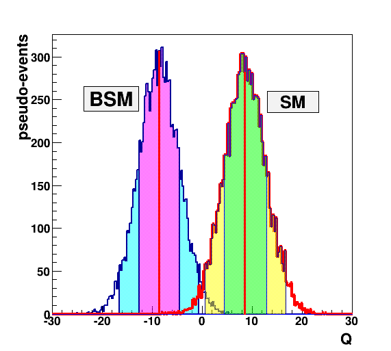
Using the distribution , we can determine the p-value of
excluding the alternate (BSM hypothesis)888We use the median
value of the null hypothesis to determine the p-value of the
alternate hypothesis. This corresponds to twice the p-value in the
method used in LEP. . We include the effects of backgrounds
completely but only profile over the various nuisance parameters that
arise from detector effects and selection cuts.
The results of this procedure are shown in figure 13 for the
pure BSM cases, where we show the variation of the p-value of the BSM
hypothesis against the luminosity. To assess the sensitivity of each
of the observables, we set the coupling strengths to values so that
they reproduce the SM cross-section after applying all the cuts,
i.e. , and with all other couplings
set to zero for each of these cases. This choice of couplings hence
eliminates the rate information from the analysis. We stress that this
is done to check the discriminating power of the observables under
consideration. The horizontal line indicates exclusion of the
alternate hypothesis at confidence level. A second horizontal
line is shown in some cases below the first one and this indicates
exclusion of the alternate hypothesis at confidence
level. For two of the couplings and we observe that the
likelihood constructed with the observable provides
a slightly stronger discriminant.
In both
cases we find that exclusion of the pure BSM hypothesis at
confidence level is possible with luminosity. The
coupling can be excluded with even less data with exclusion
confidence level possible with just luminosity. All
the likelihoods produce similar results in this case. This is as
expected since, the strongest discriminator for this coupling is the
transverse momentum distribution, while angular observables for
are not very different from SM predictions. An important point to note
is that we have set the couplings to very small values. This does not
correctly reproduce the Higgs partial decay widths. For example, if
the Higgs were a pseudo-scalar, then in order to reproduce the SM
decay width in decays, the coupling should have a value
. For such a large value of the coupling, the production
channel can easily rule out the pseudo-scalar hypothesis with of data.
We would like to emphasize that although a pure pseudoscalar hypothesis has been ruled out by an analysis of the Higgs decaying to four lepton channel, the same is not true for the coupling Chatrchyan:2013iaa 999While it is expected that the and couplings should not be to different, from a model independent approach it is important to test both couplings independently.. Since it is not easy to reconstruct the kinematics of the final state in the case of higgs decaying through W bosons, what we suggest is that it is possible to use only the rate information from the decay coupled with an analysis of production (as prescribed here) to easily rule out the pure pseudoscalar hypothesis for the coupling with a relatively small amount of luminosity.
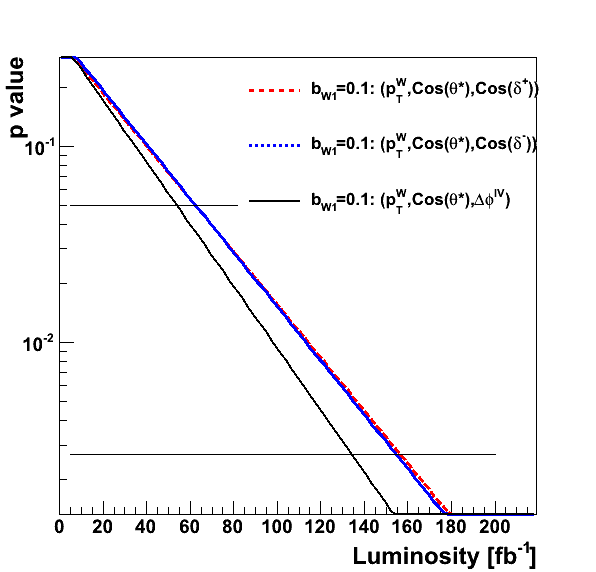
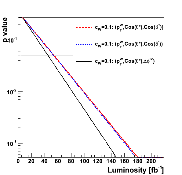
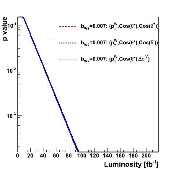
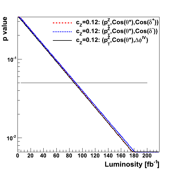
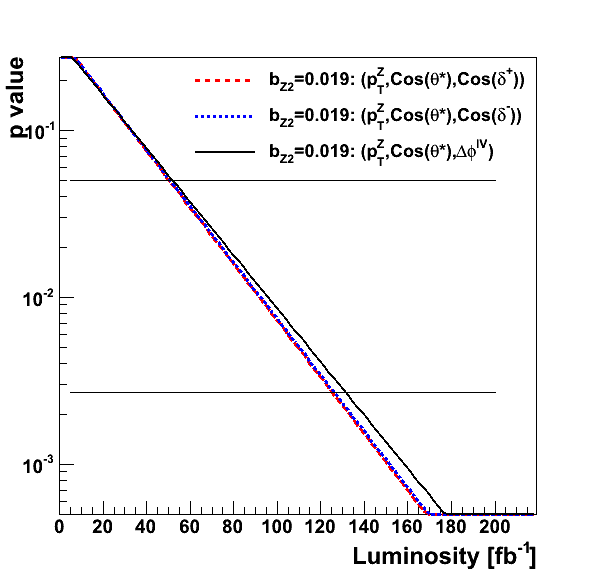
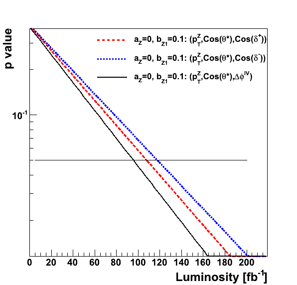
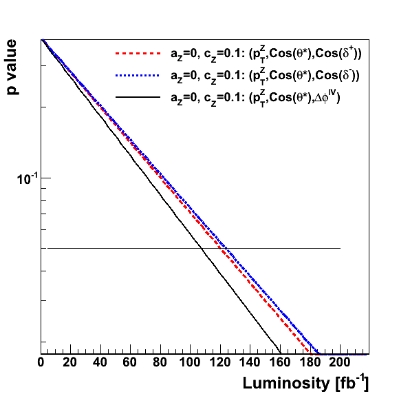
We are, however, more interested in the case where there are admixtures of the SM coupling and the BSM couplings. In figure 14 we show the variation of the p-value for the alternate hypothesis with luminosity for TeV LHC.
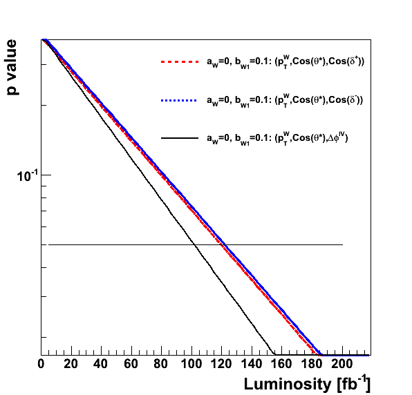
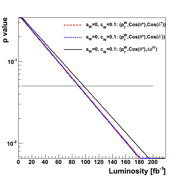
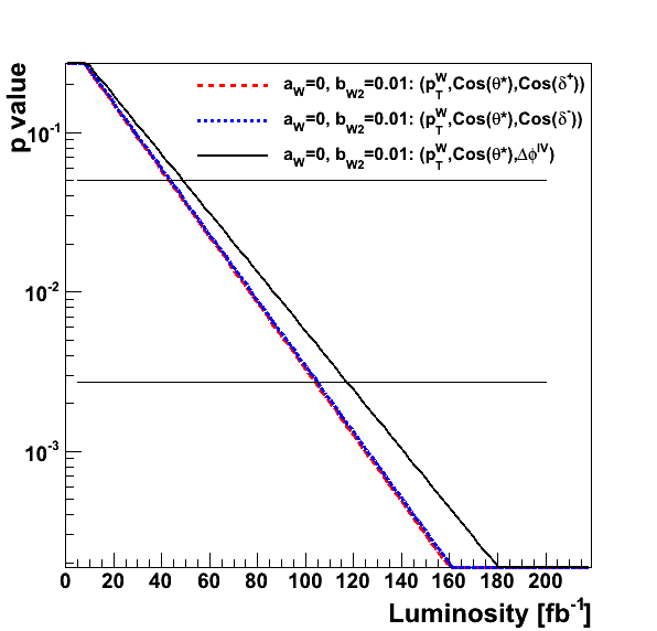
For the case when , we find that the likelihood
function constructed with does slightly better
than the other two likelihood functions. We find that the BSM
hypothesis for this choice of coupling strengths can be excluded at
confidence level with about luminosity. For the CP
violating case, , as expected, the two likelihood
functions constructed with and
appear to be the strongest discriminators with confidence level
exclusion of the BSM hypothesis is possible with about of
data. Finally for the case when , we observe, once again, that those likelihoods
constructed with and do slightly
better than the likelihood constructed with . We find that confidence level exclusion of this BSM
hypothesis possible with about luminosity.
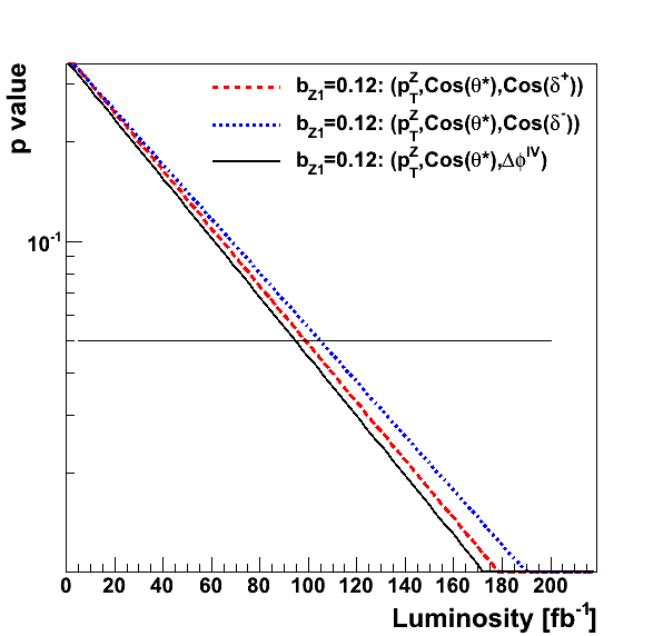
We also perform this analysis for production. The variation of the p-value of the alternate hypothesis with luminosity for a TeV LHC is shown in figure 15. Once again we compare the results of three different likelihood functions constructed out of three different combination of observables, namely , and . In contrast to production we find that all three likelihoods have a discriminating power not very different from one another. The smaller cross-section for production implies that the luminosities at which various hypotheses can be excluded is higher than for the corresponding hypotheses in production. The luminosities at which we find exclusion of the BSM hypothesis at confidence level are as follows:
-
•
, with all other couplings set to zero : .
-
•
, with all other couplings set to zero : .
-
•
, with all other couplings set to zero : .
-
•
, with all other couplings set to zero : .
-
•
, with all other couplings set to zero : .
-
•
, with all other couplings set to zero : .
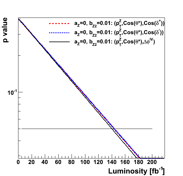
The luminosities listed in this section are all within the projected value of
for the LHC CMS:2013xfa .
We reiterate here that an analysis of the vertex in the
production mode was not conceived before due to the small
cross-section in this channel. We have shown that such an analysis is
indeed possible. The increased acceptance to BSM physics to the
cuts employed in a boosted analysis plays a crucial role in improving
the sensitivity of production to BSM physics. We have constructed observables
that are linearly sensitive to BSM couplings. Further,
in this section we have shown that our observables are quite
powerful and exclusion of various BSM hypotheses is possible with a
relatively small amount of data.
The importance of our analysis is that it provides a direct method of studying the
vertex. As mentioned earlier, other production modes such as VBF and do not provide
clean probes of the same101010For example, currently, CMS manages to exclude the pure pseudoscalar hypothesis at only CL using the
decay channel with leptonic final states Chatrchyan:2013iaa ..
It should be noted that a likelihood
analysis has several nuisance parameters (from detector effects and
selection cuts) that are a source of uncertainties in this
analysis. In order to reduce the uncertainties in probing anomalous
couplings, we look at the possibility of constructing asymmetries in
the next section. This is best suited for the CP violating case where
it is easy to construct asymmetries that would vanish in case of CP
conservation. Note that it is possible to construct asymmetries that are non-zero for the SM and are also
linear in the anomalous couplings 111111For an , see for example ref. Biswal:2005fh . However, here we focus our attention on CP-violation.
5 Asymmetries
In this section, we define asymmetry parameters related to the angular
observables of section 3. There are a number of
motivations for this. Firstly, asymmetry parameters defined in terms
of ratios are typically theoretically cleaner than kinematic
distributions, due to cancellation of PDF and scale uncertainties, as
well as reduced sensitivity to radiative corrections. They are also
experimentally easier and cleaner to measure, being related to simple
counting experiments, recording the number of events in well defined
regions of phase space.
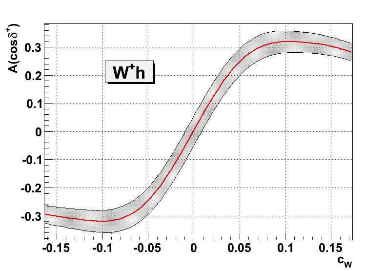
Such asymmetries can be constructed using the observables and / or defined in eq. (8). In this section we will consider the asymmetry constructed out of the observable only121212We have checked that the analogous asymmetry constructed out of the observable gives similarly large values for the asymmetry. This is expected since these two observables, as described earlier, are correlated. as follows. For events (tagged using the sign of the decay lepton) one defines
| (12) |
defining minus this quantity for events. For , we find the value of this asymmetry, after applying all selection cuts, to be for production. We also verify that the value of the asymmetry for all other cases (BSM, SM and backgrounds) is less that which is within the statistical uncertainty limits of our procedure and can be safely assumed to be vanishing. We emphasize that the vanishing of this asymmetry holds true even after including detector effects. This makes it a robust observable to probe CP violation. Since the transverse momentum cuts increase the acceptance of the BSM vertex, the value of the asymmetry depends on this kinematic cut. The asymmetry also depends on rapidity cuts since the observable depends on the cross-product of the Higgs and gauge boson momenta. We perform a simple parton level analysis of production with the decaying leptonically and the Higgs decaying to a b-quark pair. In order to mimic the cuts of a boosted analysis, we apply the following cuts at the parton level:
-
1.
Transverse momentum of the leptons GeV; rapidity ; separation from b-quarks , where .
-
2.
Missing transverse energy GeV.
-
3.
Transverse momentum of the b-quarks GeV; rapidity ; separation between b-quarks .
-
4.
Transverse momentum of reconstructed Higgs GeV.
-
5.
Transverse momentum of , GeV and .
-
6.
A b-tagging efficiency of is used and both b-jets are tagged.
We note that the value of the asymmetry calculated at the parton level
is in very good agreement with the asymmetry calculated using the full
boosted analysis simulation described in the previous sections
131313We have only tested this for three specific values of .. We
evaluate the variation of this asymmetry with the strength of the
coupling using a parton level analysis. The variation of this
asymmetry is shown in figure 16. We see that the sign of the
asymmetry depends on the sign of . We also observe that the
asymmetry peaks for a value of while a minima is
observed for . The extrema signify regions where the
interference plays an important role. For larger values of the
quadratic term (in the matrix element squared) starts contributing
more strongly to the total cross-section, thus reducing the value of
this asymmetry. However, this would correspond to a kinematic region
where one no longer trusts the effective theory framework.
In production, with the asymmetry is found to
be , an order of magnitude less than the asymmetry in case
of production. The much smaller value is due to the presence of
different vector and axial-vector couplings of the quarks and leptons
with the Z boson, as explained earlier.
Stronger probes of CP violation in the vertex can be found in ref. Godbole:2007cn .
6 Conclusion
The ongoing attempts to pin down the nature of the recently discovered
Higgs-like particle constitute a major global effort in contemporary
particle physics. In this paper, we have considered the associated
production of the Higgs with a massive gauge boson at the LHC as an
alternative to VBF production or Higgs decays, in probing anomalous contributions to
the vertex. Similar analyses in VBF can be quite difficult due
to large backgrounds and our inability to reconstruct the final state
momenta. Furthermore, in VBF production there is a significant
contribution from the vertex, reducing the ability to cleanly
distinguish this from the vertex. We have shown that such a
separation is indeed possible in production, despite the smaller
cross-section. This has been made possible with the use of modern
jet-substructure techniques. Consistent with previous
studies Djouadi:2013yb ; Ellis:2012xd ; Englert:2012ct , we find
that the very same selection criteria that are applied to eliminate
backgrounds, also enhance the sensitivity to BSM physics. This is
ultimately due to the additional momentum factors that correct the
vertices in an effective theory framework, which boost the Higgs
to higher transverse momenta on average.
Building on the preliminary work of ref. Godbole:2013saa , we
constructed angular observables that are sensitive to new physics. To
test the ability of these observables to probe the tensor structure of
the vertex, we performed a log likelihood analysis. Three
dimensional likelihood functions were constructed with different
combinations of the observables. We found that with a relatively small
amount of data (less than luminosity), it is possible to
exclude all the different cases of couplings we have considered. For
example we found that the CP-violating case could be
excluded at confidence level with luminosity
for TeV LHC.
Finally we constructed an asymmetry that is sensitive to the amount of
CP violation in interactions. The asymmetry vanishes for all
CP-conserving cases - in particular, it is zero in the SM, such that
any non-zero measurement consitutes unambiguous discovery of new
physics. We checked that the asymmetry is robust against
hadronization, radiation and detector effects.
The results of our paper merit further investigation, including implementation in future experimental analyses. We furthermore anticipate other useful applications that may result from combining jet substructure methods with polarisation ideas. Work in this regard is ongoing.
Acknowledgments
DJM and CDW are supported by the UK Science and Technology Facilities Council (STFC). RMG wishes to thank the Department of Science and Technology, Government of India, for support under grant no. SR/S2/JCB-64/2007. DJM and CDW thank the Indian Institute of Science for their hospitality while part of this work was carried out.
Appendix A Matrix elements for production
In this appendix, we collect the matrix elements for production
at leading order, including the effects of the higher-dimensional
operators described in section 1.
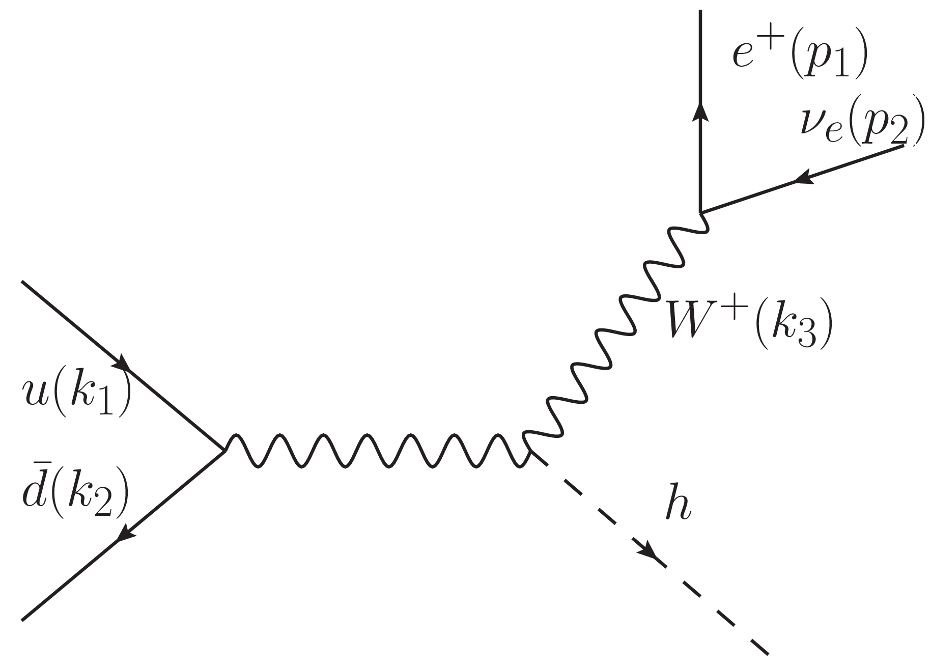
We evaluate the squared matrix element for the Feynman diagram shown in figure 17. We do not consider decay of the Higgs boson since we assume it to be spin zero and therefore its decay products will not carry information about the vertex. We evaluate the matrix element squared for this process. We use the following notation to identify parts of the matrix element that are proportional to each of the anomalous couplings of eqs. (1, 2).
| (13) |
where are the matrix elements generated from the coupling with coefficient . In keeping with the philosophy of the effective field theory approach, we keep only terms which are at most linear in the BSM couplings (constituting the interference of the BSM physics with the SM). Quadratic terms would necessitate the inclusion also of dimension eight operators. The results are:
| (14) | ||||
| (15) | ||||
| (16) | ||||
| (17) |
Here with the Levi-Civita tensor, and
corresponds to the propagators for the W bosons. Note that the SM contribution is included in eq. (14).
References
- (1) ATLAS Collaboration Collaboration, G. Aad et al., Observation of a new particle in the search for the Standard Model Higgs boson with the ATLAS detector at the LHC, Phys.Lett. B716 (2012) 1–29, [arXiv:1207.7214].
- (2) CMS Collaboration Collaboration, S. Chatrchyan et al., Observation of a new boson at a mass of 125 GeV with the CMS experiment at the LHC, Phys.Lett. B716 (2012) 30–61, [arXiv:1207.7235].
- (3) J. Espinosa, C. Grojean, M. Muhlleitner, and M. Trott, Fingerprinting Higgs Suspects at the LHC, JHEP 1205 (2012) 097, [arXiv:1202.3697].
- (4) J. Ellis and T. You, Global Analysis of Experimental Constraints on a Possible Higgs-Like Particle with Mass 125 GeV, JHEP 1206 (2012) 140, [arXiv:1204.0464].
- (5) J. Ellis and T. You, Global Analysis of the Higgs Candidate with Mass 125 GeV, JHEP 1209 (2012) 123, [arXiv:1207.1693].
- (6) J. R. Espinosa, M. Muhlleitner, C. Grojean, and M. Trott, Probing for Invisible Higgs Decays with Global Fits, JHEP 1209 (2012) 126, [arXiv:1205.6790].
- (7) T. Corbett, O. Eboli, J. Gonzalez-Fraile, and M. Gonzalez-Garcia, Constraining anomalous Higgs interactions, Phys.Rev. D86 (2012) 075013, [arXiv:1207.1344].
- (8) J. Espinosa, C. Grojean, M. Muhlleitner, and M. Trott, First Glimpses at Higgs’ face, JHEP 1212 (2012) 045, [arXiv:1207.1717].
- (9) A. Azatov, R. Contino, and J. Galloway, Model-Independent Bounds on a Light Higgs, JHEP 1204 (2012) 127, [arXiv:1202.3415].
- (10) M. Montull and F. Riva, Higgs discovery: the beginning or the end of natural EWSB?, JHEP 1211 (2012) 018, [arXiv:1207.1716].
- (11) M. Klute, R. Lafaye, T. Plehn, M. Rauch, and D. Zerwas, Measuring Higgs Couplings from LHC Data, Phys.Rev.Lett. 109 (2012) 101801, [arXiv:1205.2699].
- (12) A. Azatov, R. Contino, and J. Galloway, Contextualizing the Higgs at the LHC, arXiv:1206.3171.
- (13) Y. Gao, A. V. Gritsan, Z. Guo, K. Melnikov, M. Schulze, et al., Spin determination of single-produced resonances at hadron colliders, Phys.Rev. D81 (2010) 075022, [arXiv:1001.3396].
- (14) S. Choi, . Miller, D.J., M. Muhlleitner, and P. Zerwas, Identifying the Higgs spin and parity in decays to Z pairs, Phys.Lett. B553 (2003) 61–71, [hep-ph/0210077].
- (15) J. Ellis and D. S. Hwang, Does the ‘Higgs’ have Spin Zero?, JHEP 1209 (2012) 071, [arXiv:1202.6660].
- (16) A. De Rujula, J. Lykken, M. Pierini, C. Rogan, and M. Spiropulu, Higgs look-alikes at the LHC, Phys.Rev. D82 (2010) 013003, [arXiv:1001.5300].
- (17) K. Odagiri, On azimuthal spin correlations in Higgs plus jet events at LHC, JHEP 0303 (2003) 009, [hep-ph/0212215].
- (18) C. Buszello, I. Fleck, P. Marquard, and J. van der Bij, Prospective analysis of spin- and CP-sensitive variables in at the LHC, Eur.Phys.J. C32 (2004) 209–219, [hep-ph/0212396].
- (19) A. Bredenstein, A. Denner, S. Dittmaier, and M. Weber, Precise predictions for the Higgs-boson decay / 4 leptons, Phys.Rev. D74 (2006) 013004, [hep-ph/0604011].
- (20) P. Bhupal Dev, A. Djouadi, R. Godbole, M. Muhlleitner, and S. Rindani, Determining the CP properties of the Higgs boson, Phys.Rev.Lett. 100 (2008) 051801, [arXiv:0707.2878].
- (21) U. De Sanctis, M. Fabbrichesi, and A. Tonero, Telling the spin of the ’Higgs boson’ at the LHC, Phys.Rev. D84 (2011) 015013, [arXiv:1103.1973].
- (22) J. Ellis, V. Sanz, and T. You, Prima Facie Evidence against Spin-Two Higgs Impostors, Phys.Lett. B726 (2013) 244–250, [arXiv:1211.3068].
- (23) R. Boughezal, T. J. LeCompte, and F. Petriello, Single-variable asymmetries for measuring the ‘Higgs’ boson spin and CP properties, arXiv:1208.4311.
- (24) D. Stolarski and R. Vega-Morales, Directly Measuring the Tensor Structure of the Scalar Coupling to Gauge Bosons, Phys.Rev. D86 (2012) 117504, [arXiv:1208.4840].
- (25) J. Ellis, D. S. Hwang, V. Sanz, and T. You, A Fast Track towards the ‘Higgs’ Spin and Parity, JHEP 1211 (2012) 134, [arXiv:1208.6002].
- (26) A. Djouadi, R. Godbole, B. Mellado, and K. Mohan, Probing the spin-parity of the Higgs boson via jet kinematics in vector boson fusion, Phys.Lett. B723 (2013) 307–313, [arXiv:1301.4965].
- (27) R. Godbole, D. J. Miller, K. Mohan, and C. D. White, Boosting Higgs CP properties via VH Production at the Large Hadron Collider, arXiv:1306.2573.
- (28) J. Ellis, V. Sanz, and T. You, Associated Production Evidence against Higgs Impostors and Anomalous Couplings, Eur.Phys.J. C73 (2013) 2507, [arXiv:1303.0208].
- (29) R. Godbole, C. Hangst, M. Muhlleitner, S. Rindani, and P. Sharma, Model-independent analysis of Higgs spin and CP properties in the process , Eur.Phys.J. C71 (2011) 1681, [arXiv:1103.5404].
- (30) M. Muhlleitner, R. Godbole, C. Hangst, S. Rindani, and P. Sharma, Analysis of Higgs spin and CP properties in a model-independent way in , Frascati Phys.Ser. 54 (2012) 188–197.
- (31) E. Boos, V. Bunichev, M. Dubinin, and Y. Kurihara, Higgs boson signal at complete tree level in the SM extension by dimension-six operators, arXiv:1309.5410.
- (32) Y. Sun, X.-F. Wang, and D.-N. Gao, CP mixed property of the Higgs-like particle in the decay channel , arXiv:1309.4171.
- (33) M. B. Einhorn and J. Wudka, Higgs-Boson Couplings Beyond the Standard Model, arXiv:1308.2255.
- (34) I. Anderson, S. Bolognesi, F. Caola, Y. Gao, A. V. Gritsan, et al., Constraining anomalous HVV interactions at proton and lepton colliders, arXiv:1309.4819.
- (35) E. Masso and V. Sanz, Limits on Anomalous Couplings of the Higgs to Electroweak Gauge Bosons from LEP and LHC, Phys.Rev. D87 (2013), no. 3 033001, [arXiv:1211.1320].
- (36) D. T. Nhung, M. Muhlleitner, J. Streicher, and K. Walz, Higher Order Corrections to the Trilinear Higgs Self-Couplings in the Real NMSSM, JHEP 1311 (2013) 181, [arXiv:1306.3926].
- (37) LHC Higgs Cross Section Working Group Collaboration, S. Heinemeyer et al., Handbook of LHC Higgs Cross Sections: 3. Higgs Properties, arXiv:1307.1347.
- (38) C. Delaunay, G. Perez, H. de Sandes, and W. Skiba, Higgs Up-Down CP Asymmetry at the LHC, Phys.Rev. D89 (2014) 035004, [arXiv:1308.4930].
- (39) C. Delaunay, T. Golling, G. Perez, and Y. Soreq, Charming the Higgs, Phys.Rev. D89 (2014) 033014, [arXiv:1310.7029].
- (40) F. Maltoni, K. Mawatari, and M. Zaro, Higgs characterisation via vector-boson fusion and associated production: NLO and parton-shower effects, Eur.Phys.J. 74 (2014) 2710, [arXiv:1311.1829].
- (41) H. Belusca-Maito, Effective Higgs Lagrangian and Constraints on Higgs Couplings, arXiv:1404.5343.
- (42) M. Gavela, J. Gonzalez-Fraile, M. Gonzalez-Garcia, L. Merlo, S. Rigolin, et al., CP violation with a dynamical Higgs, arXiv:1406.6367.
- (43) A. Biekoetter, A. Knochel, M. Kraemer, D. Liu, and F. Riva, Vices and Virtues of Higgs EFTs at Large Energy, arXiv:1406.7320.
- (44) W. Buchmuller and D. Wyler, Effective Lagrangian Analysis of New Interactions and Flavor Conservation, Nucl.Phys. B268 (1986) 621.
- (45) R. Contino, M. Ghezzi, C. Grojean, M. Muhlleitner, and M. Spira, Effective Lagrangian for a light Higgs-like scalar, JHEP 1307 (2013) 035, [arXiv:1303.3876].
- (46) B. Grzadkowski, M. Iskrzynski, M. Misiak, and J. Rosiek, Dimension-Six Terms in the Standard Model Lagrangian, JHEP 1010 (2010) 085, [arXiv:1008.4884].
- (47) S. Banerjee, S. Mukhopadhyay, and B. Mukhopadhyaya, Higher dimensional operators and LHC Higgs data : the role of modified kinematics, Phys.Rev. D89 (2014) 053010, [arXiv:1308.4860].
- (48) J. Ellis, V. Sanz, and T. You, Complete Higgs Sector Constraints on Dimension-6 Operators, JHEP 1407 (2014) 036, [arXiv:1404.3667].
- (49) N. Desai, D. K. Ghosh, and B. Mukhopadhyaya, CP-violating HWW couplings at the Large Hadron Collider, Phys.Rev. D83 (2011) 113004, [arXiv:1104.3327].
- (50) S. Bolognesi, Y. Gao, A. V. Gritsan, K. Melnikov, M. Schulze, et al., On the spin and parity of a single-produced resonance at the LHC, Phys.Rev. D86 (2012) 095031, [arXiv:1208.4018].
- (51) Y. Chen, A. Falkowski, I. Low, and R. Vega-Morales, New Observables for CP Violation in Higgs Decays, arXiv:1405.6723.
- (52) CMS Collaboration Collaboration, S. Chatrchyan et al., Measurement of Higgs boson production and properties in the WW decay channel with leptonic final states, JHEP 1401 (2014) 096, [arXiv:1312.1129].
- (53) CMS Collaboration Collaboration, Constraints on anomalous HVV interactions using H to 4l decays, Tech. Rep. CMS-PAS-HIG-14-014, CERN, Geneva, 2014.
- (54) S. e. a. Dawson, Higgs Working Group Report of the Snowmass 2013 Community Planning Study, ArXiv e-prints (Oct., 2013) [arXiv:1310.8361].
- (55) Measurements of the properties of the higgs-like boson in the four lepton decay channel with the atlas detector usi ng 25 fb−1 of proton-proton collision data, Tech. Rep. ATLAS-CONF-2013-013, CERN, Geneva, Mar, 2013.
- (56) Properties of the higgs-like boson in the decay h to zz t o 4l in pp collisions at sqrt s =7 and 8 tev, Tech. Rep. CMS-PAS-HIG-13-002, CERN, Geneva, 2013.
- (57) CMS Collaboration Collaboration, S. Chatrchyan et al., Study of the Mass and Spin-Parity of the Higgs Boson Candidate Via Its Decays to Z Boson Pairs, Phys.Rev.Lett. 110 (2013) 081803, [arXiv:1212.6639].
- (58) CMS Collaboration Collaboration, S. e. a. Chatrchyan, Study of the mass and spin-parity of the higgs boson candidate via its decays to boson pairs, Phys. Rev. Lett. 110 (Feb, 2013) 081803.
- (59) (CMS Collaboration) Collaboration, S. e. a. Chatrchyan, Measurement of the properties of a higgs boson in the four-lepton final state, Phys. Rev. D 89 (May, 2014) 092007.
- (60) D0 Collaboration Collaboration, V. M. Abazov et al., Constraints on spin and parity of the Higgs boson in final states, arXiv:1407.6369.
- (61) CMS Collaboration Collaboration, Constraints on Anomalous HWW Interactions using Higgs boson decays to W+W- in the fully leptonic final state, Tech. Rep. CMS-PAS-HIG-14-012, CERN, Geneva, 2014.
- (62) T. Plehn, D. L. Rainwater, and D. Zeppenfeld, Determining the structure of Higgs couplings at the LHC, Phys.Rev.Lett. 88 (2002) 051801, [hep-ph/0105325].
- (63) V. Hankele, G. Klamke, D. Zeppenfeld, and T. Figy, Anomalous Higgs boson couplings in vector boson fusion at the CERN LHC, Phys.Rev. D74 (2006) 095001, [hep-ph/0609075].
- (64) J. R. Andersen, K. Arnold, and D. Zeppenfeld, Azimuthal Angle Correlations for Higgs Boson plus Multi-Jet Events, JHEP 1006 (2010) 091, [arXiv:1001.3822].
- (65) J. R. Andersen, V. Del Duca, and C. D. White, Higgs Boson Production in Association with Multiple Hard Jets, JHEP 0902 (2009) 015, [arXiv:0808.3696].
- (66) . Miller, D.J., S. Choi, B. Eberle, M. Muhlleitner, and P. Zerwas, Measuring the spin of the Higgs boson, Phys.Lett. B505 (2001) 149–154, [hep-ph/0102023].
- (67) T. Han and J. Jiang, CP violating Z Z H coupling at e+ e- linear colliders, Phys.Rev. D63 (2001) 096007, [hep-ph/0011271].
- (68) S. S. Biswal, D. Choudhury, R. M. Godbole, and Mamta, Role of polarization in probing anomalous gauge interactions of the Higgs boson, Phys.Rev. D79 (2009) 035012, [arXiv:0809.0202].
- (69) S. S. Biswal and R. M. Godbole, Use of transverse beam polarization to probe anomalous VVH interactions at a Linear Collider, Phys.Lett. B680 (2009) 81–87, [arXiv:0906.5471].
- (70) S. Dutta, K. Hagiwara, and Y. Matsumoto, Measuring the Higgs-Vector boson Couplings at Linear Collider, Phys.Rev. D78 (2008) 115016, [arXiv:0808.0477].
- (71) LHeC Study Group Collaboration, J. Abelleira Fernandez et al., A Large Hadron Electron Collider at CERN: Report on the Physics and Design Concepts for Machine and Detector, J.Phys. G39 (2012) 075001, [arXiv:1206.2913].
- (72) S. S. Biswal, R. M. Godbole, B. Mellado, and S. Raychaudhuri, Azimuthal Angle Probe of Anomalous Couplings at a High Energy Collider, Phys.Rev.Lett. 109 (2012) 261801, [arXiv:1203.6285].
- (73) J. M. Butterworth, A. R. Davison, M. Rubin, and G. P. Salam, Jet substructure as a new Higgs search channel at the LHC, Phys.Rev.Lett. 100 (2008) 242001, [arXiv:0802.2470].
- (74) S. D. Ellis, C. K. Vermilion, and J. R. Walsh, Techniques for improved heavy particle searches with jet substructure, Phys.Rev. D80 (2009) 051501, [arXiv:0903.5081].
- (75) S. D. Ellis, C. K. Vermilion, and J. R. Walsh, Recombination Algorithms and Jet Substructure: Pruning as a Tool for Heavy Particle Searches, Phys.Rev. D81 (2010) 094023, [arXiv:0912.0033].
- (76) D. Krohn, J. Thaler, and L.-T. Wang, Jet Trimming, JHEP 1002 (2010) 084, [arXiv:0912.1342].
- (77) D. E. Soper and M. Spannowsky, Finding physics signals with shower deconstruction, Phys.Rev. D84 (2011) 074002, [arXiv:1102.3480].
- (78) D. E. Soper and M. Spannowsky, Combining subjet algorithms to enhance ZH detection at the LHC, JHEP 1008 (2010) 029, [arXiv:1005.0417].
- (79) M. Dasgupta, A. Fregoso, S. Marzani, and G. P. Salam, Towards an understanding of jet substructure, JHEP 1309 (2013) 029, [arXiv:1307.0007].
- (80) M. Dasgupta, A. Fregoso, S. Marzani, and A. Powling, Jet substructure with analytical methods, arXiv:1307.0013.
- (81) ATLAS Collaboration Collaboration, G. Aad et al., Jet mass and substructure of inclusive jets in TeV collisions with the ATLAS experiment, JHEP 1205 (2012) 128, [arXiv:1203.4606].
- (82) ATLAS Collaboration Collaboration, G. Aad et al., ATLAS measurements of the properties of jets for boosted particle searches, Phys.Rev. D86 (2012) 072006, [arXiv:1206.5369].
- (83) ATLAS Collaboration, G. Aad et al., Performance of jet substructure techniques for large- jets in proton-proton collisions at = 7 TeV using the ATLAS detector, JHEP 1309 (2013) 076, [arXiv:1306.4945].
- (84) CMS Collaboration Collaboration, S. Chatrchyan et al., Studies of jet mass in dijet and W/Z + jet events, JHEP 1305 (2013) 090, [arXiv:1303.4811].
- (85) ATLAS Collaboration Collaboration, G. Aad et al., Search for resonances decaying into top-quark pairs using fully hadronic decays in collisions with ATLAS at TeV, JHEP 1301 (2013) 116, [arXiv:1211.2202].
- (86) ATLAS Collaboration Collaboration, G. Aad et al., A search for resonances in lepton+jets events with highly boosted top quarks collected in collisions at TeV with the ATLAS detector, JHEP 1209 (2012) 041, [arXiv:1207.2409].
- (87) ATLAS Collaboration Collaboration, G. Aad et al., Search for pair production of massive particles decaying into three quarks with the ATLAS detector in TeV collisions at the LHC, JHEP 1212 (2012) 086, [arXiv:1210.4813].
- (88) ATLAS Collaboration Collaboration, G. Aad et al., Search for pair-produced massive coloured scalars in four-jet final states with the ATLAS detector in proton-proton collisions at TeV, Eur.Phys.J. C73 (2013) 2263, [arXiv:1210.4826].
- (89) CMS Collaboration Collaboration, S. Chatrchyan et al., Search for anomalous t t-bar production in the highly-boosted all-hadronic final state, JHEP 1209 (2012) 029, [arXiv:1204.2488].
- (90) CMS Collaboration Collaboration, S. Chatrchyan et al., Search for resonant production in lepton+jets events in collisions at TeV, JHEP 1212 (2012) 015, [arXiv:1209.4397].
- (91) CMS Collaboration Collaboration, S. Chatrchyan et al., Search for heavy resonances in the W/Z-tagged dijet mass spectrum in pp collisions at 7 TeV, Phys.Lett. B723 (2013) 280–301, [arXiv:1212.1910].
- (92) C. Burges and H. J. Schnitzer, Virtual Effects of Excited Quarks as Probes of a Possible New Hadronic Mass Scale, Nucl.Phys. B228 (1983) 464.
- (93) C. N. Leung, S. Love, and S. Rao, Low-Energy Manifestations of a New Interaction Scale: Operator Analysis, Z.Phys. C31 (1986) 433.
- (94) P. Artoisenet, P. de Aquino, F. Demartin, R. Frederix, S. Frixione, et al., A framework for Higgs characterisation, arXiv:1306.6464.
- (95) A. Alloul, B. Fuks, and V. Sanz, Phenomenology of the Higgs Effective Lagrangian via FeynRules, arXiv:1310.5150.
- (96) J. Alwall, M. Herquet, F. Maltoni, O. Mattelaer, and T. Stelzer, MadGraph 5 : Going Beyond, JHEP 1106 (2011) 128, [arXiv:1106.0522].
- (97) N. D. Christensen and C. Duhr, FeynRules - Feynman rules made easy, Comput.Phys.Commun. 180 (2009) 1614–1641, [arXiv:0806.4194].
- (98) A. Alloul, N. D. Christensen, C. Degrande, C. Duhr, and B. Fuks, FeynRules 2.0 - A complete toolbox for tree-level phenomenology, Comput.Phys.Commun. 185 (2014) 2250–2300, [arXiv:1310.1921].
- (99) T. Sjostrand, S. Mrenna, and P. Z. Skands, PYTHIA 6.4 Physics and Manual, JHEP 0605 (2006) 026, [hep-ph/0603175].
- (100) J. Pumplin, D. Stump, J. Huston, H. Lai, P. M. Nadolsky, et al., New generation of parton distributions with uncertainties from global QCD analysis, JHEP 0207 (2002) 012, [hep-ph/0201195].
- (101) M. Cacciari, G. P. Salam, and G. Soyez, FastJet User Manual, Eur.Phys.J. C72 (2012) 1896, [arXiv:1111.6097].
- (102) LHC Higgs Cross Section Working Group Collaboration, S. Dittmaier et al., Handbook of LHC Higgs Cross Sections: 1. Inclusive Observables, arXiv:1101.0593.
- (103) DELPHES 3 Collaboration, J. de Favereau et al., DELPHES 3, A modular framework for fast simulation of a generic collider experiment, JHEP 1402 (2014) 057, [arXiv:1307.6346].
- (104) T. Han and S. Willenbrock, QCD correction to the and total cross-sections, Phys.Lett. B273 (1991) 167–172.
- (105) H. Baer, B. Bailey, and J. Owens, O (alpha-s) Monte Carlo approach to W + Higgs associated production at hadron supercolliders, Phys.Rev. D47 (1993) 2730–2734.
- (106) J. Ohnemus and W. J. Stirling, Order alpha-s corrections to the differential cross-section for the W H intermediate mass Higgs signal, Phys.Rev. D47 (1993) 2722–2729.
- (107) S. Dittmaier, S. Dittmaier, C. Mariotti, G. Passarino, R. Tanaka, et al., Handbook of LHC Higgs Cross Sections: 2. Differential Distributions, arXiv:1201.3084.
- (108) S. Hoeche, F. Krauss, N. Lavesson, L. Lonnblad, M. Mangano, et al., Matching parton showers and matrix elements, hep-ph/0602031.
- (109) C. Englert, M. Spannowsky, and M. Takeuchi, Measuring Higgs CP and couplings with hadronic event shapes, JHEP 1206 (2012) 108, [arXiv:1203.5788].
- (110) D0 Collaboration, E. Johnson, Spin and parity in the channel at the D0 experiment, arXiv:1305.3675.
- (111) T. Han and Y. Li, Genuine CP-odd Observables at the LHC, Phys.Lett. B683 (2010) 278–281, [arXiv:0911.2933].
- (112) N. D. Christensen, T. Han, and Y. Li, Testing CP Violation in ZZH Interactions at the LHC, Phys.Lett. B693 (2010) 28–35, [arXiv:1005.5393].
- (113) C. Englert, D. Goncalves-Netto, K. Mawatari, and T. Plehn, Higgs Quantum Numbers in Weak Boson Fusion, JHEP 1301 (2013) 148, [arXiv:1212.0843].
- (114) CMS Collaboration Collaboration, Projected Performance of an Upgraded CMS Detector at the LHC and HL-LHC: Contribution to the Snowmass Process, arXiv:1307.7135.
- (115) S. S. Biswal, R. M. Godbole, R. K. Singh, and D. Choudhury, Signatures of anomalous VVH interactions at a linear collider, Phys.Rev. D73 (2006) 035001, [hep-ph/0509070].
- (116) R. M. Godbole, D. Miller, and M. M. Muhlleitner, Aspects of CP violation in the H ZZ coupling at the LHC, JHEP 0712 (2007) 031, [arXiv:0708.0458].