11email: corentin.schreiber@cea.fr 22institutetext: Institut d’Astrophysique de Paris, UMR 7095, CNRS, UPMC Univ. Paris 06, 98bis boulevard Arago, F-75014 Paris, France 33institutetext: National Optical Astronomy Observatory, 950 North Cherry Avenue, Tucson, AZ 85719, USA 44institutetext: Max-Planck-Institut für Extraterrestrische Physik (MPE), Postfach 1312, D-85741 Garching, Germany 55institutetext: Argelander-Institut für Astronomie, University of Bonn, auf dem Hägel 71, D-53121 Bonn, Germany 66institutetext: School of Astronomy and Space Sciences, Nanjing University, Nanjing, 210093, China 77institutetext: Astronomy Center, Dept. of Physics & Astronomy, University of Sussex, Brighton BN1 9QH, UK 88institutetext: Aix-Marseille Université, CNRS, LAM (Laboratoire d’Astrophysique de Marseille) UMR7326, 13388, Marseille, France 99institutetext: University of California Observatories / Lick Observatory, University of California, Santa Cruz, CA 95064 1010institutetext: Space Telescope Science Institute, Baltimore, MD, USA 1111institutetext: Department of Astronomy, University of Massachusetts, Amherst, MA 01003, USA 1212institutetext: Department of Physics, University of Oxford, Keble Road, Oxford OX1 3RH 1313institutetext: Institute for Astronomy, Astrophysics, Space Applications and Remote Sensing, National Observatory of Athens, GR-15236 Athens, Greece 1414institutetext: Institute for Astronomy, University of Hawaii, Honolulu, Hawaii, 96822, USA 1515institutetext: Canada-France-Hawaii Telescope, Kamuela, Hawaii, 96743, USA 1616institutetext: George P. and Cynthia W. Mitchell Institute for Fundamental Physics and Astronomy, Department of Physics and Astronomy, Texas A&M University, College Station, TX 77843, USA 1717institutetext: INAF – Osservatorio Astronomico di Roma, via di Frascati 33, 00040 Monte Porzio Catone, Italy 1818institutetext: Department of Physics and Astronomy, University of British Columbia, Vancouver, BC V6T 1Z1, Canada
The Herschel††thanks: Herschel is an ESA space observatory with science instruments provided by European-led Principal Investigator consortia and with important participation from NASA. view of the dominant mode of galaxy growth from to the present day
We present an analysis of the deepest Herschel images in four major extragalactic fields GOODS–North, GOODS–South, UDS, and COSMOS obtained within the GOODS–Herschel and CANDELS–Herschel key programs. The star formation picture provided by a total of individual far-infrared detections is supplemented by the stacking analysis of a mass complete sample of star-forming galaxies from the Hubble Space Telescope (HST) band-selected catalogs of the CANDELS survey and from two deep ground-based band-selected catalogs in the GOODS–North and the COSMOS-wide field to obtain one of the most accurate and unbiased understanding to date of the stellar mass growth over the cosmic history.
We show, for the first time, that stacking also provides a powerful tool to determine the dispersion of a physical correlation and describe our method called “scatter stacking”, which may be easily generalized to other experiments.
The combination of direct UV and far-infrared UV-reprocessed light provides a complete census on the star formation rates (s), allowing us to demonstrate that galaxies at to of all stellar masses () follow a universal scaling law, the so-called main sequence of star-forming galaxies. We find a universal close-to-linear slope of the – relation, with evidence for a flattening of the main sequence at high masses () that becomes less prominent with increasing redshift and almost vanishes by . This flattening may be due to the parallel stellar growth of quiescent bulges in star-forming galaxies, which mostly happens over the same redshift range. Within the main sequence, we measure a nonvarying dispersion of : at a fixed redshift and stellar mass, about of star-forming galaxies form stars at a universal rate within a factor . The specific () of star-forming galaxies is found to continuously increase from to .
Finally we discuss the implications of our findings on the cosmic history and on the origin of present-day stars: more than two-thirds of present-day stars must have formed in a regime dominated by the “main sequence” mode. As a consequence we conclude that, although omnipresent in the distant Universe, galaxy mergers had little impact in shaping the global star formation history over the last billion years.
Key Words.:
Galaxies: evolution – Galaxies: active – Galaxies: starburst – Infrared: galaxies – Methods: statistical1 Introduction
Most extremely star-forming galaxies in the local Universe are heavily dust obscured and show undeniable signs of an ongoing major merger, however such objects are relatively rare (Armus et al., 1987; Sanders & Mirabel, 1996). They have been historically classified as Luminous and Ultra Luminous InfraRed Galaxies, LIRGs and ULIRGs, based on their bolometric infrared luminosity over the wavelength range –, by and , respectively. However, they make up for only of the integral of the local IR luminosity function, the remaining fraction mainly produced by more typical isolated galaxies (Sanders & Mirabel, 1996).
More recently, studies at higher redshift showed that the LIRGs were the dominant population at (Chary & Elbaz, 2001; Le Floc’h et al., 2005), replaced by ULIRGs at (Magnelli et al., 2013). This was first interpreted as an increasing contribution of gas-rich galaxy mergers to the global star formation activity of the Universe, in qualitative agreement with the predicted and observed increase of the major merger rate (e.g., Patton et al., 1997; Le Fèvre et al., 2000; Conselice et al., 2003).
The discovery of the correlation between star formation rate () and stellar mass (), also called the “main sequence” of star-forming galaxies (Noeske et al., 2007), at (Brinchmann et al., 2004), (Noeske et al., 2007; Elbaz et al., 2007), (Daddi et al., 2007; Pannella et al., 2009; Rodighiero et al., 2011; Whitaker et al., 2012) – (Daddi et al., 2009; Magdis et al., 2010; Heinis et al., 2013; Pannella et al., 2014) and even up to (e.g., Stark et al., 2009; Bouwens et al., 2012; Stark et al., 2013; González et al., 2014; Salmon et al., 2014; Steinhardt et al., 2014) suggested instead a radically new paradigm. The tightness of this correlation is indeed not consistent with frequent random bursts induced by processes like major mergers of gas-rich galaxies, and favors more stable star formation histories (Noeske et al., 2007).
Furthermore, systematic studies of the dust properties of the “average galaxy” at different redshifts show that LIRGs at and ULIRGs at bear close resemblance to normal star-forming galaxies at . In particular, in spite of having star formation rates (s) higher by orders of magnitude, they appear to share similar star-forming region sizes (Rujopakarn et al., 2011), polycyclic aromatic hydrocarbon (PAH) emission lines equivalent widths (Pope et al., 2008; Fadda et al., 2010; Elbaz et al., 2011; Nordon et al., 2012), to far-infrared (FIR) luminosity () ratios (Díaz-Santos et al., 2013), and universal FIR spectral energy distributions (SEDs) (Elbaz et al., 2011). Only outliers above the – correlation (usually called “starbursts”, Elbaz et al., 2011) show signs of different dust properties: more compact geometry (Rujopakarn et al., 2011), excess of (Elbaz et al., 2011), deficit (Díaz-Santos et al., 2013), increased effective dust temperature (Elbaz et al., 2011; Magnelli et al., 2014), and PAH deficit (Nordon et al., 2012; Murata et al., 2014), indicating that these starburst galaxies are the true analogs of local LIRGs and ULIRGs. In this paradigm, the properties of galaxies are no longer most closely related to their rest-frame bolometric luminosities, but rather to their excess compared to that of the main sequence.
This could mean that starburst galaxies are actually triggered by major mergers, but that the precise mechanism that fuels the remaining vast majority of “normal” galaxies is not yet understood. Measurements of galactic gas reservoirs yield gas fractions evolving from about in the local Universe (Leroy et al., 2008) up to at (Tacconi et al., 2010; Daddi et al., 2010; Geach et al., 2011; Magdis et al., 2012; Saintonge et al., 2013; Santini et al., 2014; Genzel et al., 2014, Béthermin et al. 2014, submitted). Compared to the observed , this implies gas-consumption timescales that are much shorter than the typical duty cycle of most galaxies. It is thus necessary to replenish the gas reservoirs of these galaxies in some way. Large volume numerical simulations (Dekel et al., 2009a) have shown that streams of cold gas from the intergalactic medium can fulfill this role, allowing galaxies to keep forming stars at these high but steady rates. Since the amount of gas accreted through these “cold flows” is directly linked to the matter density of the intergalactic medium, this also provides a qualitative explanation for the gradual decline of the from to the present day (e.g., Davé et al., 2011).
This whole picture relies on the existence of the main sequence. However, actual observations of the – correlation at rely mostly on ultraviolet-derived star formation rates, which need to be corrected by large factors to account for dust extinction (Calzetti et al., 1994; Madau et al., 1998; Meurer et al., 1999; Steidel et al., 1999). These corrections, performed using the UV continuum slope and assuming an extinction law, are uncertain and still debated. Although dust-corrected s are able to match more robust estimators on average in the local Universe (Calzetti et al., 1994; Meurer et al., 1999) and beyond (e.g., Pannella et al., 2009; Overzier et al., 2011; Rodighiero et al., 2014), it has been shown for example that these corrections cannot recover the full star formation rate of the most active objects (Goldader et al., 2002; Buat et al., 2005; Elbaz et al., 2007; Rodighiero et al., 2011; Wuyts et al., 2011; Penner et al., 2012; Oteo et al., 2013; Rodighiero et al., 2014). More recently, several studies have pointed toward an evolution of the calibration between the UV slope and UV attenuation as a function of redshift, possibly due to changes in the ISM properties (e.g., Pannella et al., 2014; Castellano et al., 2014) or even as a function of environment (Koyama et al., 2013). It is therefore possible that using UV-based estimates modifies the normalization of the main sequence, and/or its dispersion. In particular, it could be that the tight scatter of the main sequence observed at high redshift (e.g., Bouwens et al., 2012; Salmon et al., 2014) is not real but induced by the use of such s, thereby questioning the very existence of a main sequence at these epochs. Indeed, a small scatter is a key ingredient without which the main sequence loses its meaning.
Infrared telescopes allow us to measure the bolometric infrared luminosity of a galaxy (), a robust star formation tracer (Kennicutt, 1998). Unfortunately, they typically provide observations of substantially poorer quality (both in angular resolution and typical depth) compared to optical surveys. The launch of the Spitzer space telescope (Werner et al., 2004) was a huge step forward, as it allowed us to detect for the first time moderately luminous objects at high redshifts () in the mid-infrared (MIR) thanks to the MIPS instrument (Rieke et al., 2004). It was soon followed by the Herschel space telescope (Pilbratt et al., 2010), which provided better constraints on the spectrum of the dust emission by observing in the FIR with the PACS (Poglitsch et al., 2010) and SPIRE instruments (Griffin et al., 2010).
Nevertheless only the most luminous star-forming objects can be detected at high redshifts, yielding strongly biased samples (Elbaz et al., 2011). In particular, most galaxies reliably detected with these instruments at are very luminous starbursts, making it difficult to study the properties of “normal” galaxies at these epochs. So far only a handful of studies have probed in a relatively complete manner the Universe at with IR facilities (e.g., Heinis et al., 2014; Pannella et al., 2014) and most of what we know about normal galaxies at is currently based on UV light alone (Daddi et al., 2009; Stark et al., 2009; Bouwens et al., 2012; Stark et al., 2013; González et al., 2014; Salmon et al., 2014).
Here we take advantage of the deepest data ever taken with Herschel in the Great Observatories Origins Deep Survey (GOODS, PI: D. Elbaz), covering the GOODS–North and GOODS–South fields, and the Cosmic Assembly Near-Infrared Deep Extragalactic Legacy Survey (CANDELS, PI: M. E. Dickinson) covering a fraction of the Ultra-Deep Survey111This field is also known as the Subary XMM Deep Survey (SXDS) field. (UDS) and Cosmic Evolution Survey (COSMOS) fields, to infer stricter constraints on the existence and relevance of the main sequence in the young Universe up to . To do so, we first construct a mass-selected sample with known photometric redshifts and stellar masses and then isolate star-forming galaxies within it. We bin this sample in redshift and stellar mass and stack the Herschel images. This allows us to infer their average , and thus their s. We then present a new technique we call “scatter stacking” to measure the dispersion around the average stacked , taking nondetected galaxies into account. Finally, we cross-match our sample with Herschel catalogs to study individually detected galaxies.
In the following, we assume a CDM cosmology with , , and a Salpeter (1955) initial mass function (IMF), to derive both star formation rates and stellar masses. All magnitudes are quoted in the AB system, such that .
2 Sample and observations
| Field | Areaa | NIR () | ||||||
|---|---|---|---|---|---|---|---|---|
| () | ( | ( | ( | ( | ( | |||
| GN | ||||||||
| GS | – | |||||||
| UDS | – | |||||||
| COSMOS | ||||||||
| -CANDELS | – | – | ||||||
| -UVISTA | – | — | — | — |
(a) This is the sky coverage of our sample, and may be smaller than the nominal area of the detection image.
We use the ultra-deep -band catalogs provided by the CANDELS–HST team (Grogin et al., 2011; Koekemoer et al., 2011) in three of the CANDELS fields, namely GOODS–South (GS Guo et al., 2013), UDS (Galametz et al., 2013), and COSMOS (Nayyeri et al. in prep.). With the GOODS–North (GN) CANDELS catalog not being finalized at the time of writing, we fall back to a ground-based -band catalog. To extend our sample to rarer and brighter objects, we also take advantage of the much wider area provided by the -band imaging in the COSMOS field acquired as part of the UltraVISTA program (UVISTA). In the following, we will refer to this field as “COSMOS UltraVISTA”, while the deeper but smaller region observed by CANDELS will be called “COSMOS CANDELS”.
Using either the or the as the selection band will introduce potentially different selection effects. In practice, these two bands are sufficiently close in wavelengths that one does not expect major differences to arise: if anything, the -band catalogs are potentially more likely to be mass-complete, since this band will probe the rest-frame optical up to higher redshifts. However these catalogs are ground based, and lack both angular resolution and depth when compared to the HST -band data. It is thus necessary to carefully estimate the mass completeness level of each catalog, and only consider mass-complete regimes in the following analysis.
All these fields were selected for having among the deepest Herschel observations, which are at the heart of the present study, along with high-quality, multi-wavelength photometry in the UV to NIR. The respective depths of each catalog are listed in Table 1. We next present the details of the photometry and source extraction of each field.
2.1 GOODS–North
GOODS–North is one of the fields targeted by the CANDELS–HST program, and the last to be observed. Consequently, the data reduction was delayed compared to the other fields and there was no available catalog when we started this work. We thus use the ground-based -band catalog presented in Pannella et al. (2014), which is constructed from the deep CFHT WIRCAM -band observations of Wang et al. (2010). This catalog contains 20 photometric bands from the NUV to IRAC and was built using SExtractor (Bertin & Arnouts, 1996) in dual image mode, with the -band image as the detection image. Fluxes are measured within a aperture on all images, and the effect of varying point spread function (PSF) and / or seeing is accounted for using PSF-matching corrections. Per-object aperture corrections to total are provided by the ratio of the FLUX_AUTO as given by SExtractor and the aperture -band flux. This results in a angular resolution catalog of sources and a limiting magnitude of .
The -band image extends over , but only the central area is covered by Spitzer and Herschel. We therefore only keep the sources that fall inside the coverage of those two instruments, i.e., objects in . We also remove stars identified either from the SExtractor flag CLASS_STAR for bright enough objects (), or using the color-color diagram (Daddi et al., 2004). Our final sample consists of galaxies, of which are brighter than the limiting magnitude, with spectroscopic redshifts.
The Herschel images in both PACS and SPIRE were obtained as part of the GOODS–Herschel program (Elbaz et al., 2011). The source catalog of Herschel and Spitzer MIPS are taken from the public GOODS–Herschel DR1. Herschel PACS and SPIRE flux densities are extracted using PSF fitting at the position of MIPS priors, themselves extracted from IRAC priors. SPIRE and flux densities are obtained by building a reduced prior list out of the detections. This procedure, described in more detail in Elbaz et al. (2011), yields MIPS and Herschel detections ( in any PACS band or in SPIRE, following Elbaz et al., 2011) that we could cross-match to the -band catalog using their IRAC positions.
2.2 GOODS–South, UDS, & COSMOS CANDELS
In GOODS–South, UDS and COSMOS CANDELS we use the official CANDELS catalogs presented, respectively, in Guo et al. (2013) (version ), Galametz et al. (2013) (version ) and Nayyeri et al. (in prep.) (version ). They are built using SExtractor in dual image mode, using the HST -band image as the detection image to extract the photometry at the other HST bands. The ground-based and Spitzer photometry is obtained with TFIT (Laidler et al., 2007). The HST photometry was measured using the FLUX_ISO from SExtractor and corrected to total magnitudes using either the FLUX_BEST or FLUX_AUTO measured in the band, while the ground-based and Spitzer photometry is already “total” by construction. These catalogs gather photometric bands in GOODS–South, in UDS, and in COSMOS, ranging from the band to IRAC , for a total of (respectively and ) sources, (respectively and ) of which have a spectroscopic redshift. The -band exposure in the fields is quite heterogeneous, the limiting magnitude ranging from to in GOODS–South, to in UDS, and to in COSMOS, but it always goes much deeper than the available ground-based photometry. These extreme depths can also become a problem, especially when dealing with sources so faint that they are significantly detected in the HST images only. The SED of these objects is so poorly constrained that we cannot robustly identify them as galaxies, or compute accurate photometric redshifts. To solve this issue, one would like to only keep sources that have a sufficient wavelength coverage, e.g., imposing a significant detection in at least ten UV to NIR bands, but this would introduce complex selection effects. Here we decide to only keep sources that have an -band magnitude brighter than . This ensures that the median number of UV to NIR bands for each source (along with the th and th percentiles) is , and , respectively, as compared to , and when using the whole catalogs.
As for GOODS–North, we remove stars using a combination of morphology and classification, and end up with (respectively and ) galaxies with in (respectively and ).
In both UDS and COSMOS, the Herschel PACS and SPIRE images were taken as part of the CANDELS–Herschel program, and are slightly shallower than those in the two GOODS fields. The MIPS images, however, are clearly shallower, since they reach a noise level of approximately (), as compared to the in GOODS. In COSMOS, however, the MIPS map contains a “deep” region (Sanders et al., 2007) that covers roughly half of the COSMOS CANDELS area with a depth of about .
In those two fields, sources are extracted with the same procedure as in GOODS–North (Inami et al. in prep). These catalogs provide, respectively, and MIPS sources as well as and Herschel detections within the HST coverage. Since the IRAC priors used in the source extraction come directly from the CANDELS catalog, no cross-matching has to be performed.
The Herschel images in GOODS–South come from three separate programs. The PACS images are the result of the combined observation of both GOODS–Herschel and PEP (Lutz et al., 2011), while SPIRE images were obtained as part of the HerMES program (Oliver et al., 2012). The PACS fluxes are taken from the public PEP DR1 catalog (Magnelli et al., 2013), and were extracted using the same procedure as in GOODS–North. For the SPIRE fluxes, we downloaded the individual level-2 data products covering the full ECDFS from the Herschel ESA archive222http://www.cosmos.esa.int/web/herschel/science-archive and reduced them following the same procedure as the other sets of SPIRE data used in GOODS and CANDELS–Herschel. This catalog provides MIPS and Herschel detections within the HST coverage, which were cross matched to the CANDELS catalog using their IRAC positions.
2.3 COSMOS UltraVISTA
Only a small region of the COSMOS field has been observed within the CANDELS program. For the remaining area, we have to rely on ground-based photometry. To this end, we consider two different -band catalogs, both based on the UltraVISTA DR1 (McCracken et al., 2012).
The first catalog, presented in Muzzin et al. (2013b), is built using SExtractor in dual image mode, with the -band image as detection image. The photometry in the other bands is extracted using PSF-matched images degraded to a common resolution of and an aperture of , except for the Spitzer bands and GALEX. Here, an alternative cleaning method is used, where nearby sources are first subtracted using the PSF-convolved -band profiles ( band for GALEX), then the photometry of the central source is measured inside an aperture of . In both cases, aperture fluxes are corrected to total using the ratio of FLUX_AUTO and aperture -band flux. In the end, the catalog contains 30 photometric bands ranging from GALEX FUV to IRAC (we did not use the photometry), for a total of objects and a limiting magnitude of . As for the CANDELS fields, stars are excluded using a combination of morphological and classification, resulting in a final number of galaxies within , of which are brighter than the limiting magnitude, with having spectroscopic redshifts.
The second catalog, presented in Ilbert et al. (2013), is very similar in that, apart from missing GALEX and Subaru , it uses the same raw images and was also built with SExtractor. The difference lies mostly in the extraction of IRAC fluxes. Here, and for IRAC only, SExtractor is used in dual image mode, with the Subaru -band image as the detection image. Since the IRAC photometry was not released along with the rest of the photometry, we could not directly check the consistency of the two catalogs, nor use this photometry to derive accurate galaxy properties. Nevertheless, the photometric catalog comes with a set of photometric redshifts and stellar masses that we can use as a consistency check. These were built using a much more extensive but private set of spectroscopic redshifts, and are thus expected to be of higher quality. A direct comparison of the two photometric redshift estimations shows a constant relative scatter of below . At higher redshifts, the scatter increases to because of the ambiguity between the Balmer and Lyman breaks. This ambiguity arises because of the poor wavelength coverage caused by the shallow depths of these surveys, but it takes place in a redshift regime where our results are mostly based on the deeper, and therefore more robust, CANDELS data. We also checked that redoing our analysis with Ilbert et al.’s catalog yielded very similar results in the mass-complete regimes.
Finally, while the Spitzer MIPS imaging is the same as that in COSMOS CANDELS, the Herschel PACS images in this wide field were taken as part of the PEP program, at substantially shallower depth (Lutz et al., 2011). The Spitzer MIPS and Herschel PACS photometry are taken from the public PEP DR1 catalog333http://www.mpe.mpg.de/ir/Research/PEP/DR1, itself based on the MIPS catalog of Le Floc’h et al. (2009), yielding MIPS and PACS detections successfully cross-matched to the first band catalog.
2.4 Photometric redshifts and stellar masses
Photometric redshifts (photo-) and stellar masses are derived using the procedure described in Pannella et al. (2014). Briefly, photo-s are computed using EAZY444http://code.google.com/p/eazy-photoz. (Brammer et al., 2008) in its standard setup. Global photometric zero points are adjusted iteratively by comparing the photo-s to the available spectroscopic redshifts (spec-), and minimizing the difference between the two. We emphasize that, although part of these adjustments are due to photometric calibration issues, they also originate from defects in the adopted SED template library. To estimate the quality of the computed photo-s, we request that the odds computed by EAZY, which is the estimated probability that the true redshift lies within (Benítez, 2000), be larger than . A more stringent set of criteria is adopted in COSMOS CANDELS, because of the lower quality of the photometric catalog. To prevent contamination of our sample from issues in the photometry, we prefer to be more conservative and only keep and impose that the of the fit be less than to remove catastrophic fits. The median is respectively , , , , and in GOODS–North, GOODS–South, UDS CANDELS, COSMOS CANDELS, and COSMOS UltraVISTA. We stress however that the representativeness of this accuracy also depends on the spectroscopic sample. In COSMOS UltraVISTA, for example, we only have spec-s for the brightest objects, hence those that have the best photometry. Fainter and more uncertain sources thus do not contribute to the accuracy measurement, which is why the measured value is so low. Lastly, although we use these spec-s to calibrate our photo-s, we do not use them afterwards in this study. The achieved precision of our photo-s is high enough for our purposes, and the selection functions of all spectroscopic surveys we gather here are very different, if not unknown. To avoid introducing any incontrollable systematic, we therefore decide to consistently use photo-s for all our sample.
Stellar masses are derived using FAST555http://astro.berkeley.edu/~mariska/FAST.html (Kriek et al., 2009), adopting Salpeter (1955) IMF666Using another IMF would systematically shift both our and s by approximately the same amount, and therefore would not affect the shape of the main sequence., the Bruzual & Charlot (2003) stellar population synthesis model and assuming that all galaxies follow delayed exponentially declining777Other star formation histories were considered, in particular with a constant or exponentially declining . Selecting all galaxies from to , no systematic offset is found, while the scatter evolves mildly from at to at . star formation histories (SFHs), parametrized by with . Dust extinction is accounted for assuming the Calzetti et al. (2000) law, with a grid ranging from to . Metallicity is kept fixed and equal to . We assess the quality of the stellar mass estimate with the reduced of the fit, only keeping galaxies for which .
2.5 Rest-frame luminosities and star formation rates
Star formation rates are typically computed by measuring the light of young OB stars, which emit the bulk of their light in the UV. However this UV light is most of the time largely absorbed by the interstellar dust, and re-emitted in the IR as thermal radiation. To obtain the total of a galaxy, it is therefore necessary to combine the light from both the UV and the IR.
Rest-frame luminosities in the FUV (), , , and bands are computed with EAZY by convolving the best-fit SED model from the stellar mass fit with the filter response curves. The FUV luminosity is then converted into uncorrected for dust attenuation using the formula from Daddi et al. (2004), i.e.,
| (1) |
The infrared luminosity is computed following the procedure of Elbaz et al. (2011). We fit the Herschel flux densities with CE01 templates, and compute from the best-fit template. In this procedure, photometric points below rest-frame are not used in the fit since this is a domain that is potentially dominated by active galactic nuclei (AGN) torus emission, and not by star formation (e.g., Mullaney et al., 2011). We come back to this issue in section 2.6. This IR luminosity is, in turn, converted into dust-reprocessed using the formula from Kennicutt (1998)
| (2) |
The total is finally computed as the sum of and . The above two relations are derived assuming a Salpeter (1955) IMF and assume that the remained constant over the last .
A substantial number of galaxies in this sample ( in the CANDELS fields, in COSMOS UltraVISTA) are detected by Spitzer MIPS but not by . Although for these galaxies we only have a single photometric point in the MIR, we can still infer accurate monochromatic s using the original calibration of the CE01 library. This calibration is valid up to , as shown in Elbaz et al. (2011), hence we only use MIPS-derived s for sources not detected by Herschel over this redshift range. Although there exist other calibrations that are applicable to higher redshifts (e.g., Elbaz et al., 2011; Wuyts et al., 2011), we do not know how they would impact the measurement of the scatter of the main sequence. We therefore prefer not to use them and discard the measurements above . Galaxies not detected in the MIR () or FIR have no individual estimates and are only used for stacking. When working with detections alone (section 4.6), this obviously leads to an selected sample and is taken into account by estimating the completeness.
Lastly, there are some biases that can affect our estimates of from the IR. In particular, the dust can also be heated by old stars that trace the total stellar mass content rather than the star formation activity (e.g., Salim et al., 2009). Because of the relatively low luminosity of these stars, this will most likely be an issue for massive galaxies with low star formation activity, i.e., typically quiescent galaxies (see, e.g., Appendix A where we analyze such cases). Since we remove these galaxies from our sample, we should not be affected by this bias. This is also confirmed by the excellent agreement of IR based estimates with those obtained from the radio emission (e.g., Pannella et al., 2014), the latter not being affected by the light of old stars.
2.6 A mass-complete sample of star-forming galaxies
| Field | All galaxiesa | SFb | Spec-c | Herscheld |
|---|---|---|---|---|
| GN | ||||
| GS | ||||
| UDS | ||||
| COSMOS | ||||
| -CANDELS | ||||
| -UVISTA |
(a) Number of galaxies in our mass-complete NIR sample, removing stars, spurious sources, and requiring Spitzer and Herschel coverage. (b) Final subsample of good quality galaxies classified as star-forming with the criterion (see section 2.6). (c) Subsample of galaxies with a spectroscopic redshift (various sources, see catalog papers for references). (d) Subsample of galaxies with a detection in any Herschel band, requiring significance in PACS or in SPIRE (following Elbaz et al., 2011).
We finalize our sample by selecting actively star-forming galaxies. Indeed, the observation of a correlation between mass and only applies to galaxies that are still forming stars, and not to quiescent galaxies. The latter are not evolving anymore and pile up at high stellar masses with little to no detectable signs of star formation. Nevertheless, they can still show residual IR emission due to the warm inter stellar medium (ISM). This cannot be properly accounted for with the CE01 library, and will be misinterpreted as an tracer.
Several methods exist to exclude quiescent galaxies. The most obvious is to select galaxies based on their specific (). Indeed, quiescent galaxies have very low by definition, and they are preferentially found at high . Therefore, they will have very low compared to star-forming galaxies. This obviously relies on the very existence of the correlation between and , and removing galaxies with too low would artificially create the correlation even where it does not exist. On the other hand, selecting galaxies based on their alone would destroy the correlation, even where it exists (Rodighiero et al., 2011; Lee et al., 2013). It is therefore crucial that the selection does not apply directly to any combination of or . Furthermore, these methods require that an accurate is available for all galaxies, and this is something we do not have since most galaxies are not detected in the mid- or far-IR. We must therefore select star-forming galaxies based on information that is available for all the galaxies in our sample, i.e., involving optical photometry only.
There are several color-magnitude or color-color criteria that are designed to accomplish this. Some, like the approach (Daddi et al., 2004), are based on the observed photometry and are thus very simple to compute, but they also select a particular redshift range by construction. This is not desirable for our sample, and we thus need to use rest-frame magnitudes. Color-magnitude diagrams (e.g., versus -band magnitude as in Baldry et al., 2004) tend to wrongly classify some of the red galaxies as passive, while they could also be red because of high dust attenuation. Since high mass galaxies suffer the most from dust extinction (Pannella et al., 2009), it is thus likely that color-magnitude selections would have a nontrivial effect on our sample. It is therefore important to use another color to disentangle galaxies that are red because of their old stellar populations and those that are red because of dust extinction.
To this end, Williams et al. (2009) devised the selection, based on the corresponding color-color diagram introduced in Wuyts et al. (2007). It uses the color, similar to the from the standard color-magnitude diagram, but combines it to the color to break the age–dust degeneracy. Although the bimodality stands out clearly on this diagram, the locus of the passive cloud has been confirmed by Williams et al. (2009) using a sample of massive galaxies in the range with little or no [O II] line emission, while the active cloud falls on the Bruzual & Charlot (2003) evolutionary track for a galaxy with constant . One can then draw a dividing line that passes between those two clouds to separate one population from the other. We use the following definition, at all redshifts and stellar masses:
| (3) |
This definition differs by only magnitude compared to that of Williams et al. (2009). Rest-frame colors can show offsets of similar order from one catalog to another, because of photometric coverage and uncertainties in the zero-point corrections. It is thus common to adopt slightly different definitions to account for these effects (see e.g., Cardamone et al., 2010; Whitaker et al., 2011; Brammer et al., 2011; Strazzullo et al., 2013; Viero et al., 2013; Muzzin et al., 2013b). In COSMOS UltraVISTA, we follow the definition given by Muzzin et al. (2013b).
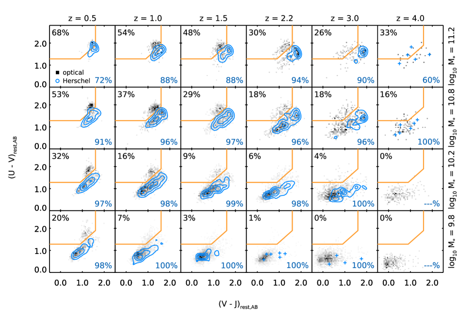
The corresponding diagram in bins of mass and redshift for the CANDELS fields is shown in Fig. 1. Here we also overplot the location of the galaxies detected by Herschel; because of the detection limit of the surveys, the vast majority of Herschel detections have high s. We therefore expect them to fall on the “active” region. This is indeed the case for the vast majority of these galaxies, even when the majority of optical sources are quiescent as is the case at and . In total, only of the galaxies in our Herschel sample are classified as passive, and about a third of those have a probability larger than to be misclassified because of uncertainties in their colors. The statistics in COSMOS UltraVISTA are similar.
The number of galaxies with reliable redshifts and stellar masses (see section 2.4) that are classified with this diagram as actively star-forming are reported in Table 2. These are the galaxies considered in the following analysis. As a check, we also analyze separately the quiescent galaxies in Appendix A.
Finally, we do not explicitly exclude known AGNs from our sample. We expect AGNs to reside in massive star-forming galaxies (Kauffmann et al., 2003; Mullaney et al., 2012; Santini et al., 2012; Juneau et al., 2013; Rosario et al., 2013). While the most luminous optically unobscured AGNs may greatly perturb the optical photometry, and therefore the measurement of redshift and stellar mass, they will also degrade the quality of the SED fitting because we have no AGN templates in our fitting libraries. This can produce an increased , hence selecting galaxies with (see section 2.4) helps remove some of these objects. Also, their point-like morphology on the detection image tends to make them look like stars, which are systematically removed from the sample. The more common moderate luminosity AGNs can still be fit properly with galaxy templates (Salvato et al., 2011). Therefore, several AGNs do remain in our sample without significantly affecting the optical SED fitting and stellar masses. Still, obscured AGNs will emit some fraction of their light in the IR through the emission of a dusty torus. To prevent pollution of our FIR measurements by the light of such dusty AGNs, we only use the photometry at rest-frame wavelengths larger than , where the contribution of the AGN is negligible (Mullaney et al., 2011). Indeed, while the most extreme AGNs may affect mid-to-far IR colors, such as -to- color, their far-IR colors are indistinguishable from that of star-forming galaxies (Hatziminaoglou et al., 2010). By rejecting the most problematic cases, and mitigating against AGN contribution to the IR, we aim to remove severe contamination while retaining a high sample completeness.
2.7 Completeness and mass functions
| Catalog | ||||||
|---|---|---|---|---|---|---|
| GN | ||||||
| CANDELSa | ||||||
| COSMOS UVISTA |
(a) These values are valid for GOODS–South, UDS, and COSMOS CANDELS, keeping all sources with .
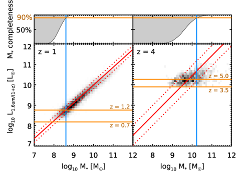
The last step before going through the analysis is to make sure that, in each stellar mass bin we will work with, as few galaxies as possible are missed because of our selection criteria. The fact that we built these samples by starting from an NIR selection makes it much simpler to compute the corresponding mass completeness: the stellar mass of a galaxy at a given redshift is indeed well correlated with the luminosity in the selection band (either or ), as illustrated in Fig. 2, the scatter around the correlation being caused by differences of age, attenuation, and to some extent flux uncertainties and -correction. From our sample, we can actually see by looking at this correlation with various bands (, , and IRAC channels 1 and 2) that this scatter is minimal () when probing the rest-frame , but it reaches dex in the rest-frame UV (). While this value is of course model dependent, it stresses the importance of having high-quality NIR photometry, especially the Spitzer IRAC bands (observed –).
To estimate the mass completeness, we decided to use an empirical approach, where we do not assume any functional form for the true mass function. Instead, we directly compute the completeness assuming that, at a given redshift, the stellar mass is well estimated by a power law of the luminosity (measured either from the observed or band), i.e., , plus a Gaussian scatter in log space. We fit this power law and estimate the amplitude of the scatter using the detected galaxies, as shown in Fig. 2. Using this model (red solid and dotted lines) and knowing the limiting luminosity in the selection band (orange horizontal lines), we can estimate how many galaxies we miss at a given stellar mass, using, e.g., a Monte Carlo simulation. At a given stellar mass, we generate a mock population of galaxies with uniform redshift distribution within the bin and estimate what would be their luminosity in the selection band by using the above relation and adding a Gaussian scatter to the logarithm of the luminosity. The completeness is then computed as the fraction of galaxies that have a luminosity greater than the limiting luminosity at the considered redshift. We consider our catalogs as “complete” when the completeness reaches at least .
The same procedure is used on COSMOS UltraVISTA and GOODS–North separately, and the estimated completeness levels are all reported in Table 3. We compared the values obtained in GOODS–North with those reported in Pannella et al. (2014), where the completeness is estimated following Rodighiero et al. (2010) using a stellar population model. The parameters of the model chosen in Pannella et al. (2014) are quite conservative, and their method consistently yields mass limits that are on average higher than ours. In COSMOS UltraVISTA, we obtain values similar to that of Muzzin et al. (2013a).
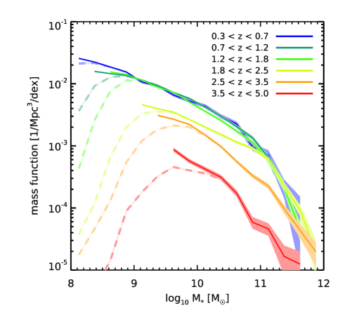
Finally, we build stellar mass functions by simply counting the number of galaxies in bins of redshift and stellar masses in the three CANDELS fields that are -band selected, and normalize the counts by the volume that is probed. These raw mass functions are presented in Fig. 3 as dashed lines. Assuming that the counts follow a Schechter-like shape, i.e., rising with a power law toward low stellar mass, the incompleteness of our sample is clearly visible. We then use the estimated completeness (top panel in Fig. 2) to correct the stellar mass functions. Here, we limit ourselves to reasonable corrections of at most a factor two in order not to introduce too much uncertainty in the extrapolation. The resulting mass functions are shown as solid lines in Fig. 3, with shaded areas showing the Poisson noise. The obtained mass functions are in good agreement with those already published in the literature (e.g., Ilbert et al., 2013).
3 Deriving statistical properties of star-forming galaxies
Because of the limitations of the Herschel surveys (the result of photometric or confusion noise), we cannot derive robust individual s for all the sources in our sample (see section 2.5). Indeed, the fraction of star-forming galaxies detected in the FIR ranges from 80% at and , to almost 0% for and . Above , the completeness in FIR detections reaches better than only above and up to . Below this mass and above that redshift, the FIR completeness is lower than –.
We overcome these limitations by stacking the Herschel images. Stacking is a powerful and routinely used technique that combines the signal of multiple sources at various positions on the images, known from deeper surveys (see, e.g., Dole et al., 2006, where it was first applied to FIR images). This effectively increases the signal to noise ratio of the measurement, allowing us to probe fainter fluxes than can be reached by the usual source extraction. The price to pay is that we lose information about each individual source, and only recover statistical properties of the considered sample. Commonly, this method is used to determine the average flux density of a selected population of objects. We will show in the following that it can also be used to obtain information on the flux distribution of the sample, i.e., not only its average flux, but also how much the stacked sources scatter around this average value.
This scatter is crucial information. If we measure an average correlation between and , as has been measured in several other studies at different redshifts, this correlation cannot be called a “sequence” if the sources show a large dispersion around it.
Several studies have already measured this quantity. Noeske et al. (2007) and Elbaz et al. (2007) at reported a dispersion in of around from Spitzer MIPS observations of a flux-limited sample. At , Rodighiero et al. (2011) reported , using mostly UV-derived s, while Whitaker et al. (2012) reported from Spitzer MIPS observations. These two studies tested the consistency of their estimator on average, but we do not know how they impact the measure of the dispersion. The variation found in these two studies suggests that this is indeed an issue (see for example the discussion in Speagle et al., 2014). On the one hand, UV s have to be corrected for dust extinction. If one assumes a single extinction law for the whole sample, one might artificially reduce the dispersion. On the other hand, MIPS at probes the rest-frame . While Elbaz et al. (2011) have shown that it correlates well with , this same study also demonstrates that it misses a fraction of that is proportional to the distance from the main sequence. This can also have an impact on the measured dispersion.
Here we measure for the first time the – main sequence and its dispersion with a robust tracer down to the very limits of the deepest Herschel surveys to constrain its existence and relevance at higher redshifts and lower stellar masses.
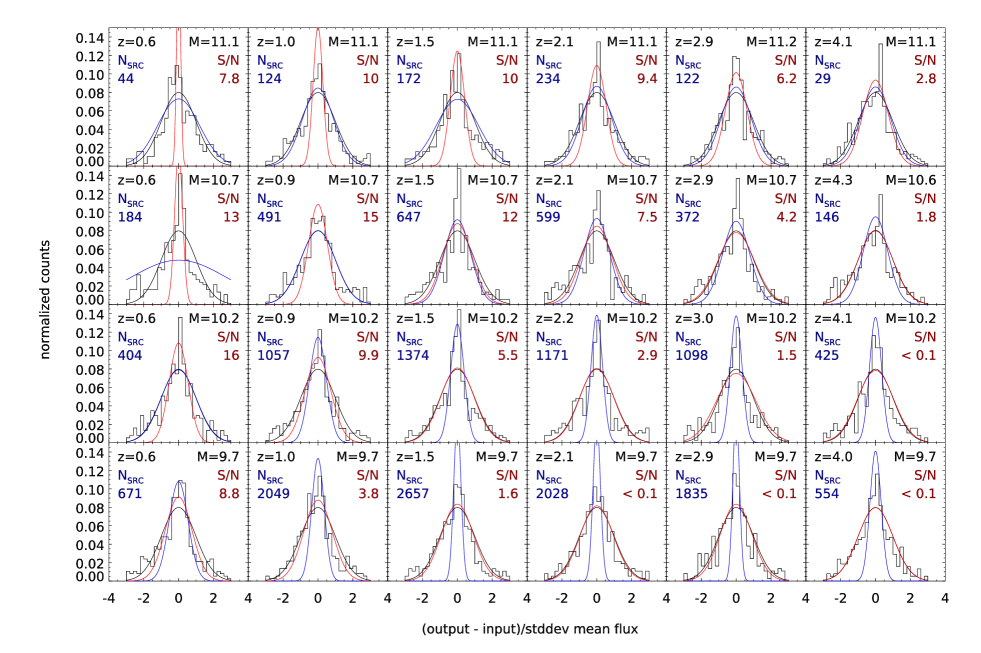
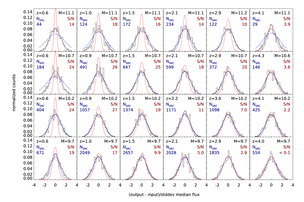
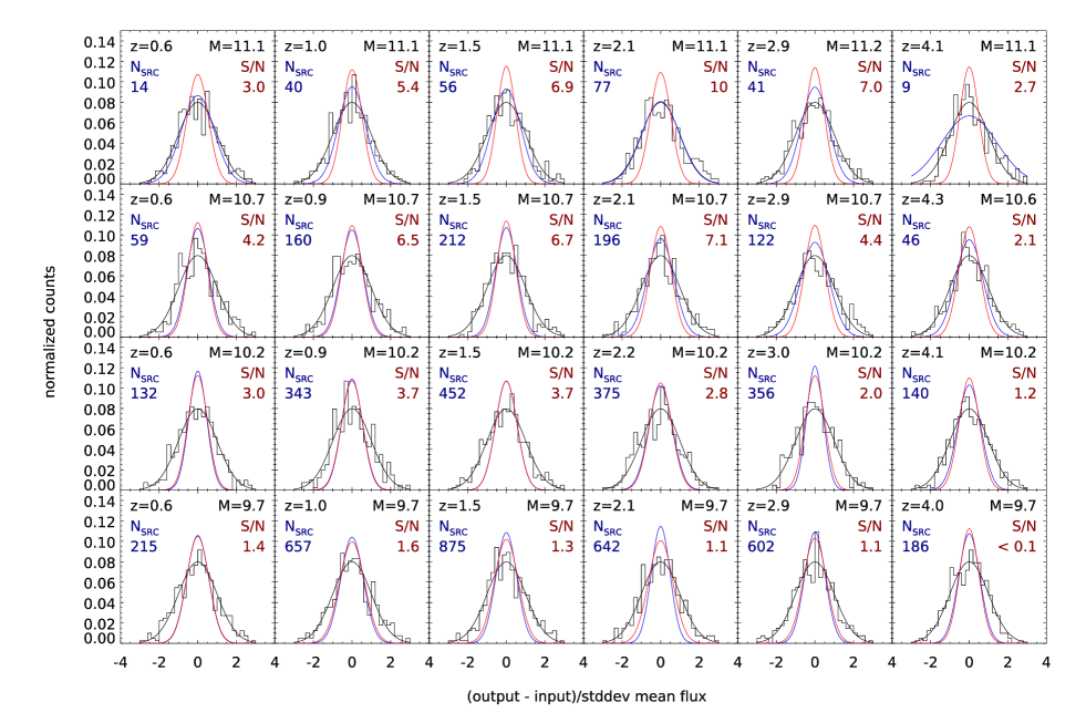
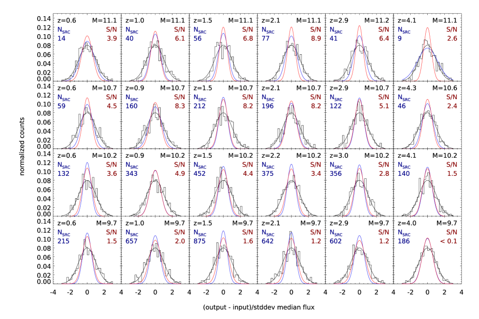
3.1 Simulated images
All the methods described in this section have been extensively tested to make sure that they are not affected by systematic biases or, if they are, to implement the necessary corrections. We conduct these tests on simulated Herschel images that we set up to be as close as possible to the real images, in a statistical sense. In other words, we reproduce the number counts, the photometric noise, the confusion noise, and the source clustering. The algorithms, the methodology, and the detailed results are described fully in Appendix B.
3.2 The stacking procedure
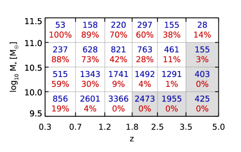
We divide our star-forming galaxy sample into logarithmic bins of stellar mass and redshift, as shown in Fig. 4, to have a reasonable number of sources in each bin. We then go to the original Herschel images of each field and extract pixel cutouts around each source in the bin, thus building a pixel cube. We choose for all Herschel bands, which is equivalent to times the full-width at half maximum (FWHM) of the PSF, and for Spitzer MIPS (), as a substantial fraction of the Spitzer flux is located in the first Airy ring. Since the maps were reduced in a consistent way across all the CANDELS fields, we can safely merge together all the sources in a given bin, allowing us to go deeper while mitigating the effects of cosmic variance.
In parallel, we also stack the sources of the COSMOS UltraVISTA catalog in the wider but shallower FIR images. These stacked values are mostly used as consistency checks, since they do not offer any advantage over those obtained in the CANDELS fields: the shallow Herschel exposure is roughly compensated by the large area, but the mass completeness is much lower.
In the literature, a commonly used method consists of stacking only the undetected sources on the residual maps, after extracting sources brighter than a given flux threshold. This removes most of the contamination from bright neighbors, and thus lowers the confusion noise for the faint sources, while potentially introducing a bias that has to be corrected. Detected and stacked sources are then combined using a weighted average (as in, e.g., Magnelli et al., 2009). We prefer here to treat both detected and undetected sources homogeneously in order not to introduce any systematic error tied to either the adopted flux threshold or the details of the source extraction procedure. Although simpler, this procedure nevertheless gives accurate results when applied to our simulated images. Indeed, the contribution of bright neighbors is a random process: although it is clear that each source suffers from a varying level of contamination, statistically they are all affected in the same way. In other words, when a sufficient number of sources are stacked, the contribution of neighbors tends to average out to the same value on all pixels, which is the contribution of galaxies to the Cosmic InfraRed Background (CIRB). But this is only true in the absence of galaxy clustering (Béthermin et al., 2010). When galaxies are clustered, there is an increased probability of finding a neighbor close to each stacked galaxy (Chary & Pope, 2010), so that will be larger toward the center of the stacked image. Kurczynski & Gawiser (2010) proposed an alternative stacking technique (implemented by Viero et al., 2013, in the SIMSTACK code) that should get rid of most of this bias, and that consists of simultaneously fitting for the flux of all sources within a given volume (i.e., in a given redshift bin). It is however less versatile, and in particular it is not capable of measuring flux dispersions. Béthermin et al. (2014, submitted) also show that is can suffer from biases coming from the incompleteness of the input catalog.
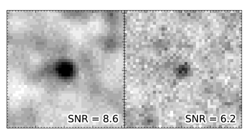
The next step is to reduce each cube into a single image by combining the pixels together. There are several ways to do this, the two most common being to compute the mean or the median flux of all the cutouts in a given pixel. The advantage of the mean stacking is that it is a linear operation, thus one can exactly understand and quantify its biases (e.g., Béthermin et al., 2010). More specifically, it can be shown that the mean stacked value corresponds to the covariance between the input source catalog and the map (Marsden et al., 2009). Median stacking, on the other hand, has the nice property of naturally filtering out bright neighbors and catastrophic outliers and thus produces cleaner flux measurements. On the down side, we show in Appendix B.1 that this measurement is systematically biased in a nontrivial way (see also White et al., 2007). Correcting for this bias requires some assumptions about the stacked flux distribution, e.g., the dispersion. Since this is a quantity we want to measure, we prefer to use mean over median stacking. An example of a mean stacked cutout from the SPIRE images is shown in Fig. 5 (left). However, in two bins at low masses and high redshifts ( and , as well as and ), the mean stacked fluxes have signal to noise ratios that are too low and thus cannot be used, while the median stacked fluxes are still robustly measured. To extend our measurement of the main sequence , we allow ourselves to use the median stacked fluxes in these particular bins only. This is actually a regime where we expect the median stacking to most closely measure the mean flux (see Appendix B.1), hence this should not introduce significant biases. Lastly, we are interested in the mode of the main sequence, which is not strictly speaking the mean we measure. We calibrated the difference between those two quantities with our simulations, and in all the following we refer to the of the main sequence as the mode of the distribution. For example, for a log-normal distribution of , this difference is about .
To measure the stacked flux, we choose to use PSF fitting in all the stacked bands. In all fields, we use the same PSFs as those used to extract the photometry of individual objects, and apply the corresponding aperture corrections. This method assumes that the stacked image is a linear combination of: 1) a uniform background; and 2) the PSF of the instrument, since none of our sources is spatially resolved. The measured flux is then obtained as the best-fit normalization factor applied to the PSF that minimizes the residuals. In practice, we simultaneously fit both the flux and the background within a fixed aperture whose radius is times the FWHM of the PSF. The advantage of this choice is that although we use less information in the fit, the background computed this way is more local, and the flux measurement is more robust against source clustering. Indeed, the amplitude of the clustering is a continuous function of angular distance: although a fraction of clustered sources will fall within a radius that is much smaller than the FWHM of the PSF and will bias our measurements no matter what, the rest will generate signal over a scale that is larger than the PSF itself, such that it will be resolved. Estimating the background within a small aperture will therefore remove the contribution of clustering coming from the largest scales.
We quantify the expected amount of flux boosting due to source physical clustering using our simulated maps. We show in Appendix B.2 that it is mostly a function of beam size, i.e., there is no effect in the PACS bands but it can boost the SPIRE fluxes by up to at . We also compare our flux extraction method to other standard approaches and show that it does reduces the clustering bias by a factor of to , while also producing less noisy flux measurements. The value of was chosen to get the lowest clustering amplitudes and flux uncertainties.
To obtain an estimate of the error on this measure, we also compute the standard deviation of the residual image (i.e., the stacked image minus the fitted source) and multiply it by the PSF error scaling factor
| (4) |
where is the number of pixels that are used in the fit, is the sum of all the pixels of the PSF model within the chosen aperture, and the sum of the squares of these pixels. This is the formal error on the linear fit performed to extract the flux (i.e., the square root of the diagonal element corresponding to the PSF in the covariance matrix), assuming that all pixels are affected by a similar uncorrelated Gaussian error of amplitude . In practice, since the PSFs that we use are all sampled by roughly the same number of pixels (approximately two times the Nyquist sampling), this factor is always close to divided by the value of the central pixel of the PSF. Intuitively, this comes from the fact that the error on the measured flux is the combination of the error on all the pixels that enter in the fit, weighted by the amplitude of the PSF. It is thus naturally lower than the error on one single pixel. In other words, using PSF fitting on these stacks allows for measuring fluxes that are twice as faint as those obtained when using only the central pixel of the image. Simple aperture photometry yields , where is the number of pixels used to estimate the background (e.g., within an annulus around the source). If is sufficiently large (), this error is lower than that obtain with our PSF fitting technique because the background is estimated independently of the flux. The price to pay is that this background is not local, hence the aperture flux will be most sensitive to clustering. Finally, if there is no clustering, PSF fitting will give the lowest errors of all methods, provided the full PSF is used in the fit. The optimal strategy is therefore always to use PSF fitting, varying the aperture within which the fit is performed depending on the presence of clustering.
To be conservative, we compute an alternative error estimate using bootstrapping: we randomly discard half of the sources, stack the remaining ones, measure the stacked flux, and repeat this procedure times. The error is then computed as the standard deviation of the measured flux in these realizations, divided by , since we only work with half of the parent sample. Using our simulated images, we show in Appendix B.3 that accurate error estimates are obtained by keeping the maximum error between and . For the SPIRE bands, however, the same simulations show that both error estimates are systematically underestimated and need to be corrected by a factor of . We demonstrate in Appendix B.3 that this comes from the fact that the error budged in the SPIRE bands is mostly generated by the random contribution of nearby sources rather than instrumental or shot noise. In this case, the error on each pixel is largely correlated with that of its neighbors, and the above assumptions do not hold.
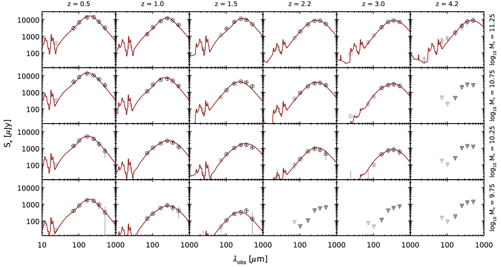
We apply the above procedure to all the redshift and stellar mass bins of Fig. 4 and stack all the MIR to FIR images, from MIPS to SPIRE . Using the measured mean fluxes, we build effective SEDs888These SEDs are effective in the sense that they are not necessarily the SED of the average galaxy in the sample: they are potentially broadened by the range of redshifts and dust temperatures of the galaxies in the stacked samples. In practice, we checked that the broadening due to the redshift distribution is negligible, and the photometry is well fitted by standard galaxy templates, as can be seen in Fig. 6. in each bin, shown in Fig. 6. We fit the Herschel photometry with CE01 templates, leaving the normalization of each template free and keeping only the best-fit, and obtain the mean . As for the individual detections, we do not use the photometry probing rest-frame wavelengths below (see section 2.5). The MIPS photometry is used as a check only. Converting the measured to with the Kennicutt (1998) relation and adding the mean observed (non-dust-corrected contribution), we obtain the mean total in each bin.
3.3 Measuring flux dispersion with scatter stacking
To measure the flux dispersion, we introduce a new method. The idea is to come back to the pixel cube and build a dispersion image by measuring the scatter of each pixel around its average value. Stacked pixels away from the center measure the background fluctuations (the combination of photometric noise and random contribution from nearby sources), while pixels in the central region show enhanced dispersion due to flux heterogeneities in the stacked population, as in Fig. 5. In particular, if all the stacked sources had the same flux, the dispersion map would be flat.
Again, this can be achieved in different ways. Computing the standard deviation of pixels is the most straightforward approach, but it suffers from similar issues as mean stacking with respect to bright neighbor contamination, in a more amplified manner because pixels are combined in quadrature. Our simulations also show that this method is not able to reliably measure high dispersion values. We thus use the median absolute deviation (MAD), which is more effective in filtering out outliers while providing the same information.
The is formally defined as the half-width of the range that is centered on the median flux and contains of the whole sample. In other words
| (5) |
where is the cumulative probability distribution function of the flux.
To interpret this value in terms of more common dispersion indicators, we will convert the to a -dispersion assuming that fluxes follow a Gaussian distribution in , i.e., a log-normal distribution in . There are two reasons that justify this choice: 1) it allows for direct comparison of our measured dispersions to the data from literature that quote standard deviations of ; and 2) log-normal distribution are good models for describing distributions in the regimes where we can actually detect individual sources (see, e.g., Rodighiero et al., 2011; Sargent et al., 2012; Gladders et al., 2013; Guo et al., 2013, and also section 4.6). For this family of distributions,
| (6) |
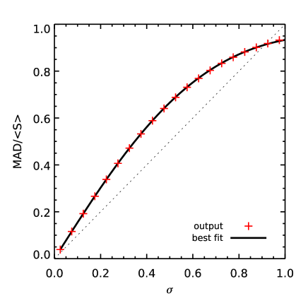
where is the complementary error function. In this case there is no analytical solution to Eq. 5, but it can be solved numerically. It turns out that one can relate the and directly to (see Fig. 7) via the following equation, which was fit on the output of the numerical analysis999This analysis was performed with Mathematica. (for ):
| (7) |
with a maximum absolute error of less than . This relation can, in turn, be inverted to obtain . Defining the “normalized” median absolute deviation , and only keeping the positive solution of Eq. 7, we obtain
| (8) |
Therefore, measuring the allows us to obtain the intrinsic log-normal flux dispersion of the stacked sample. To do so, we perform PSF fitting on the squared images (since the dispersion combines quadratically with background noise) and fit a constant background noise plus the square of the PSF on all the pixels within a fixed radius of . Here we do not use the same cut as for the flux extraction, since the MAD does not fully preserve the shape of the PSF when its pixels are low in signal to noise (see below). We thus restrain ourselves to a more central region to prevent being dominated by these faint pixels. Again, this value was chosen using the simulated maps in order to produce the least biased and least uncertain measurements.
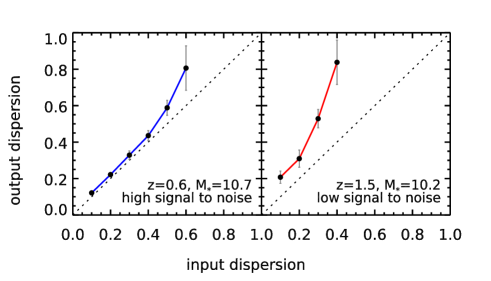
Even then, the dispersion measured with this method is slightly biased toward higher values, but this bias can be quantified and corrected in a self-consistent way with no prior information using Monte Carlo simulations. For each source in the stack, we extract another cutout at a random position in the map. We then place a fake source at the center of each random cutout, whose flux follows a log-normal distribution of width , and with a mean flux equal to that measured for the real sources. We apply our scatter stacking technique to measure the dispersion on the resulting mock flux cube, and compare it to . We repeat this procedure for different values of (from to ), and derive the relation between the intrinsic and measured dispersion. Examples are shown in Fig. 8. To average out the measurement error, we repeat this procedure times for each value of . In practice, this correction is mostly negligible, except for the lowest measured mass bins at any redshift where it reaches up to .
3.4 dispersion from scatter stacking
The procedure described in the previous section allows us to measure the log-normal flux dispersion, while we are interested in the dispersion in .
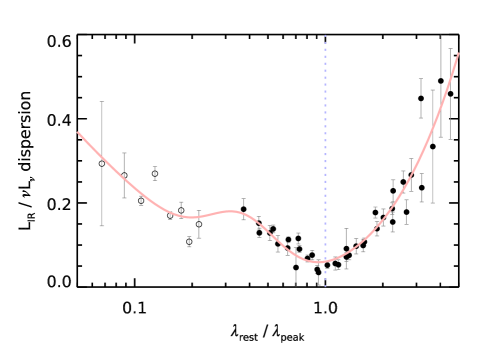
The first step is to obtain the dispersion . Using detected sources, we observe that the dispersion in of a population of galaxies having the same flux at a given redshift depends on the rest-frame wavelength probed, as illustrated in Fig. 9. The data points in this figure are produced by looking at multiple bins of redshift, and measuring the scatter of the correlation between , measured by fitting all available FIR bands, and the flux in each Herschel band converted to rest-frame luminosity (). By spanning a range of redshift, the five Herschel bands will probe a varying range of rest-frame wavelengths, allowing us to observe the behavior of the scatter with rest-frame wavelength. The smaller dispersions are found at wavelengths close to the peak of the SED, in which case the dispersion drops as low as . This is due to galaxies showing a variety of effective dust emissivities and temperatures that both influence the shape of the FIR SED, respectively longward and shortward of the peak.
Therefore, to obtain , we simply measure the flux dispersion of the Herschel band that is the closest to the peak. We thus first measure the peak wavelength from the stacked SEDs (Fig. 6), and interpolate the measured log-normal flux dispersions at . By construction, this also tends to select Herschel measurements with the highest signal to noise ratio.
One then has to combine the dispersion in with that in , since we combine both tracers to derive the total . This is not straightforward, as the two quantities are not independent (i.e., at fixed , more attenuated objects will have higher and lower ). In particular, we see on individual detections that the dispersion of is actually lower than that of alone.
To address this issue, we choose to work directly on “SFR stacks”. First, we use our observed FIR SEDs to derive monochromatic conversion factors for all bands in each of our redshift and stellar mass bins. Second, in each stacked bin, we convert all cutouts to units, using the aforementioned conversion factor and the Kennicutt (1998) relation. Third, we add to each individual cutout an additional amount of equal to the non-dust-corrected , as a centered PSF. Finally, to correct for the smearing due to the width of the redshift and mass bins, we also use our observed relation between mass, redshift, and (given below in Eq. 9) and normalize each cutout to the reference mass and redshift of the sample by adding . This last step is a small correction: it reduces the measured dispersion by only to .
We stack these cutouts and again run the dispersion measurement procedure, including the bias correction. Interpolating the measured dispersions in the five Herschel bands at as described earlier, we obtain . As expected, the difference between the flux dispersion at the peak of the SED and the dispersion is marginal, except for the lowest mass bins where it can reach . This is mainly caused by the increasing contribution of the escaping UV light to the total , as approaches unity in these bins.
A remaining bias that we do not account for in this study is the impact of errors on the photo-s and stellar masses. As pointed out in section 2.4, the measured few percent accuracy on the photo-s only applies to the bright sources, and we do not know the reliability of the fainter sources. We measure statistical uncertainties on both these quantities, but this does not take systematic errors coming from the library or gaps in the photometry into account. Intuitively, one can expect these errors to increase the dispersion, but this would be true only if the true error was purely random. It could be that our SED fitting technique is too simplistic in assuming a universal IMF, metallicity, and SFH functional form for all galaxies, and as such erases part of the diversity of the population. This could in turn decrease the measured dispersion (see discussion in Reddy et al., 2012). It is therefore important to keep in mind that our measurement is tied to the adopted modeling of stellar mass.
4 Results
4.1 The of main-sequence galaxies
The first results we present concern the evolution of the main sequence with redshift, as well as its dependence on stellar mass. In section 4.2 we start by describing the redshift evolution of the , and we then address the mass dependence of the slope of the main sequence in section 4.3.
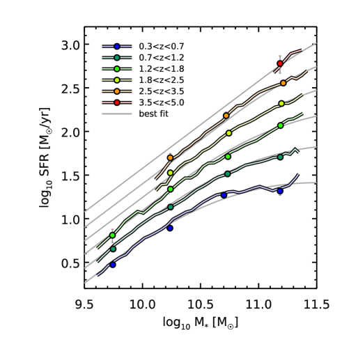
These results are summarized in Fig. 10 where, for the sake of visualization, we also run our full stacking procedure on sliding bins of mass, i.e., defining a fine grid of and selecting galaxies within mass bins of constant logarithmic width of . The data points are not independent anymore, since a single galaxy is included in the stacked sample of multiple neighboring points, but this allows us to better grasp the evolution of the main sequence with mass. These “sliding averages” of the are displayed as solid colored lines, while the points obtained with regular mass bins are shown as filled circles.
By fitting these points (filled circles only), we parametrize the of main-sequence galaxies with the following formula, defining and :
| (9) |
with , , , and . The choice of this parametrization is physically motivated: we want to explicitly describe the two regimes seen in Fig. 10 and explored in more detail in section 4.3, namely a sequence of slope unity whose normalization increases with redshift (first terms), and a “bending” that vanishes both at low masses and high redshifts (last term). The precise functional form however is arbitrary, and was chosen as the simplest expression that accurately reproduces the bending behavior. This will be used in the following as a reference for the locus of the main sequence.
4.2 Redshift evolution of the : the importance of sample selection and dust correction
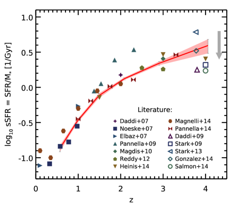
We show in Fig. 11 the evolution of () as a function of both redshift and stellar mass. Our results at are in good agreement with previous estimates from the literature, showing the dramatic increase of the with redshift. At , we still measure a rising , reaching , i.e., a mass doubling timescale of only .
At this redshift, however, our measurement is substantially higher than UV-based estimates (Daddi et al., 2009; Stark et al., 2009). More recent results (Bouwens et al., 2012; Stark et al., 2013; González et al., 2014) seem to be in better agreement, but it is important to keep in mind that these studies mostly focus on relatively low mass galaxies, i.e., typically . Therefore the quoted values only formally apply to galaxies in this range, i.e., to galaxies a factor of to times less massive than those in our sample. Extrapolating their measurements to match the mass range we are working with requires that we know the slope of the – relation. In their study, Bouwens et al. (2012) measured this slope from to at and found it to be around . Assuming that this holds for all masses, this means that we should reduce the by about to be able to compare it directly to our result. This is illustrated by the gray arrow in Fig. 11.
Previous observations of the “plateau” (Daddi et al., 2009) could be the consequence of two key issues. First, selection effects: these studies are based either on Lyman break galaxies (LBGs) or rest-frame FUV-selected samples that, while less prone to lower redshift contaminants, are likely to miss highly attenuated and thus highly star-forming galaxies. Our sample is mass-complete, so we do not suffer from such biases. Second, failure of dust extinction correction: UV-based estimates are plagued by uncertainties in dust attenuation. Most studies rely on observed correlations between UV SED features and dust attenuation that are calibrated in the local Universe, such as the – relation (Meurer et al., 1999). Recent studies tend to show that these correlations are not universal and evolve with redshift, possibly due to subsolar metallicity (Castellano et al., 2014), ISM conditions, or dust geometry (Oteo et al., 2013; Pannella et al., 2014).
4.3 Mass evolution of the and varying slope of the main sequence
It is also worth noting the dependence of the on stellar mass from Fig. 10. Low mass bins () are well fit with a slope of unity. Many studies have reported different values of this slope, ranging from to unity (Brinchmann et al., 2004; Noeske et al., 2007; Elbaz et al., 2007; Daddi et al., 2007; Santini et al., 2009; Pannella et al., 2009; Rodighiero et al., 2011). A slope of unity can be interpreted as a signature of the universality of the star formation process, since it implies a constant star formation timescale at all stellar masses, with . As suggested by Peng et al. (2010), it is also a necessary ingredient for explaining the observed shape invariance of the stellar mass function of star-forming galaxies.
We find however that the of the highest mass bin () falls systematically below the value expected for a linear relation, effectively lowering the high mass slope of the – relation to at high redshift, down to an almost flat relation at . Other studies obtain similar “broken” shapes for the – sequence (Rodighiero et al., 2010; Whitaker et al., 2012; Magnelli et al., 2014). Our results are also in very good agreement with Whitaker et al. (2014), who used a very similar approach, albeit only using MIPS for stacking.
The reason for this bending of the slope is still unknown. Abramson et al. (2014) showed that the relation between the disk mass and has a slope close to one with no sign of bending at , suggesting that the bulge plays little to no role in star formation. We will investigate if this explanation holds at higher redshifts in a forthcoming paper.
4.4 Mass evolution of the dispersion around the main sequence
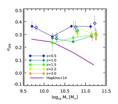
We present in Fig. 12 the evolution of the measured dispersion as a function of both redshift and stellar mass. We show our measurements only from stacking Herschel bands. Spitzer MIPS is more sensitive and thus allows measurements down to lower stellar masses, but it is less robust as an indicator. This is mostly an issue at , where the is probing the rest-frame . Elbaz et al. (2011) have shown that the luminosity correlates very well with ( scatter), except for starburst galaxies. Inferring from thus has the tendency to erase part of the starburst population, effectively reducing the observed dispersion. We checked that our results are nevertheless in good agreement between MIPS and Herschel, with MIPS derived dispersions being smaller on average by only .
As a sanity check, we also show an estimation of from individual Herschel detections. We select all galaxies in our Herschel sample that fall in a given bin of redshift and mass, and compute their offset from the main sequence , where is the average of “main sequence” galaxies given in Eq. 9. Following Elbaz et al. (2011), we call this quantity the “starburstiness”. Because of the sensitivity of Herschel, this sample is almost never complete, and is biased toward high values of : since this sample is selected, all the galaxies at low mass are starbursts. To avoid completeness issues, we remove the galaxies that have , i.e., galaxies that are below the main sequence, and compute the th percentile of the resulting distribution. By construction, this value does not need to be corrected for the width of the redshift and mass bins. However, it is only probing the upper part of the – correlation, while the stacked measurements also take undetected sources below the sequence into account. In spite of this difference, the values obtained are in very good agreement with the stacked values. There is a tendency for these to be slightly higher by on average, and this could be due to uncertainties in the individual measurements. We conclude that the distributions must be quite symmetric. This however does not rule out a “starburst” tail, i.e., a subpopulation of galaxies with an excess of star formation. Indeed, simulating a log-normal distribution of with a dispersion of and adding more sources with an excess of (following Sargent et al., 2012) gives a global dispersion measured with of , while the th percentile of the tail is , a difference of only , which is well within the uncertainties.
4.4.1 Implications for the existence of the main sequence
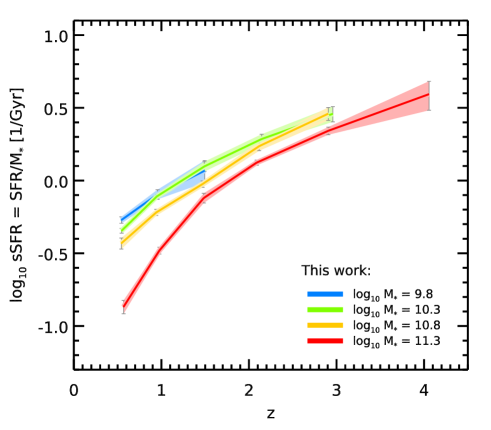
Probably the most striking feature of Fig. 12 is that remains fairly constant over a large fraction of the parameter space we explore, only increasing for the lowest redshift bin and at high stellar masses. This increase is most likely caused by the same phenomenon that bends the sequence at high stellar mass (see section 4.2, e.g., a substantial population of bulge-dominated objects that blur the correlation). On average, Herschel stacking thus gives , with a random error of , and can be considered almost constant. Doing the same analysis in COSMOS UltraVISTA consistently yields , with a random error of , showing that this result is not tied to specifics of our input -band catalogs.
More importantly, this value of means that, at a given stellar mass, of actively star-forming galaxies have the same within a factor of two. This confirms the existence of the main sequence of star-forming galaxies for all of the stellar mass range probed here and up to , i.e., over more than of the history of the universe. A more illustrative picture is shown later in Fig. 16, and we discuss the implication of this finding in section 5.1.
4.5 Contribution of the main sequence to the cosmic density
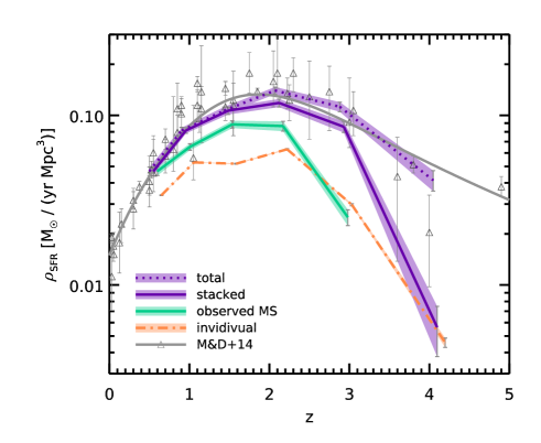
Using our stacked s, we can infer the contribution of each of our stacked bins to the cosmic star formation rate density (Lilly et al., 1996; Madau et al., 1996). To this end, we use the stellar mass functions described in section 2.7 and extrapolate our results to obtain a prediction for the total , assuming a main-sequence slope of unity for low mass galaxies, and integrating the mass functions down to (i.e., ). The results of this analysis are presented in Figs. 13 and 14, and compared to the literature compilation of Madau & Dickinson (2014) (where luminosity functions are integrated down to , and should thus match our measurements to first order).
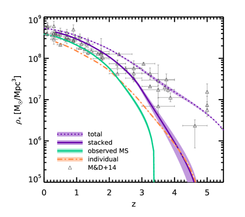
We also infer the total stellar mass density by integrating as a function of time. At each time step, we create a new population of stars whose total mass is given by , and let it evolve with time. We account for stellar mass loss using the Salpeter (1955) IMF to model the population, allowing stars to evolve and die assuming the stellar lifetimes of Bressan et al. (1993) for solar metallicity. As stars die, some of the matter is left in the form of stellar remnants that are traditionally also included in , i.e., neutron stars and white dwarfs. We parametrize the masses of these remnants following Prantzos & Silk (1998). The contribution of these remnants continuously rises with time to reach about at . The result is presented in Fig. 15.
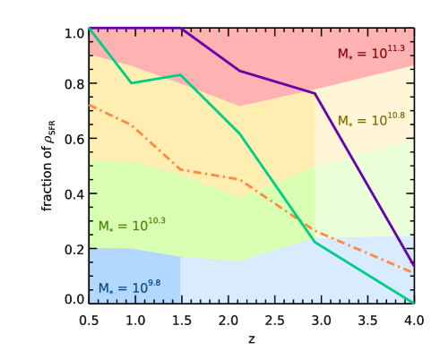
One can see from these figures that individual Herschel detections in the ultra-deep GOODS and CANDELS surveys (orange dash-dotted line) unveil about of the star formation budget below , but less than at . In total, and over the redshift range probed here, these galaxies have built of the mass of present day stars, and are thus to be considered as major actors in the stellar mass build up in the Universe. Stacking (purple line) allows us to go much deeper, since we reach almost of the total at , and accounts for of the mass of present day stars. Extrapolating our observations to lower stellar masses using the mass functions and to using the best-fit of Madau & Dickinson (2014), we obtain an estimate of the total amount of star formation in the Universe (purple dotted line). Integrating it to gives , consistent with the value reported by Cole et al. (2001) and Bell et al. (2003) (our error estimate being purely statistical).
Although the range in redshift and stellar mass over which we are able to probe the existence of the main sequence is limited, it nevertheless accounts for of the mass of present day stars. This number climbs up to if we take other studies that have observed a tight correlation down to (Brinchmann et al., 2004) into account. We show in the next section that starburst galaxies make up about of the budget in all the redshift and mass bins that we probe with individual detections, and that the remaining fraction is accounted for by a single population of “main sequence” galaxies. Subtracting these from the above , we can say that at least of the mass of present day stars was formed by galaxies belonging to the main sequence. In other words, whatever physical phenomenon shapes the main sequence is the dominant mode of star formation in galaxies.
4.6 Quantification of the role of starburst galaxies and the surprising absence of evolution of the population
4.6.1 An overview of the main sequence
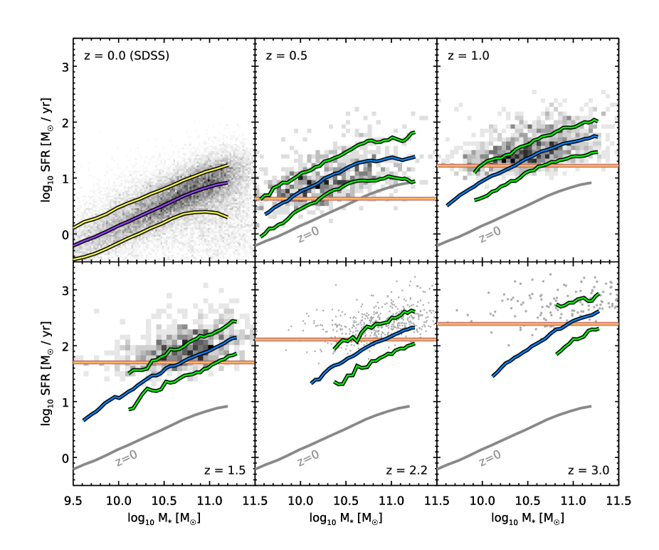
We summarize the previous results in Fig. 16. Here we show the distribution of individually detected galaxies on the – plane at various redshifts. The locus of our stacked s (solid blue lines) may not appear to coincide with the average of the detections because of the detection limit, symbolized by the horizontal dashed line. We discuss later on (in Fig. 17) the distribution of these detected sources and confirm that the stacks and the detections are in perfect agreement.
We also show for reference the sample taken from the Sloan Digital Sky Survey (SDSS DR4, Brinchmann et al., 2004) as presented in Elbaz et al. (2007). In this data set, actively star-forming galaxies are selected according to their rest-frame colors only (i.e., what is usually referred to as the “blue cloud”), and s are estimated from the dust-corrected line. These differences of observables and sample selection are likely to affect the shape of the main sequence. In particular, it is clear that the bending at high mass is less pronounced in the SDSS sample, and this is likely due to the selection. Therefore, the comparison of this data set with our own sample should be done with caution. This nevertheless resembles our own results quite closely and allows us to paint a consistent picture from to .
4.6.2 “Starburstiness” distributions
Although the depth of the Herschel surveys is limited, there is still a lot to be learned from the individually detected sources, in particular for the bright starburst galaxies. Now that we have a good definition of the main sequence, we can study these galaxies in more detail. Rodighiero et al. (2011) have used similar data in COSMOS and found that the distribution of star-forming galaxies on and off the main sequence is bimodal: a population of normal star-forming galaxies shapes the main sequence with a log-normal distribution of at a given mass, while another smaller population of “starbursts” boosts the high counts. Their work was restricted to because of the selection, so we want to extend it here to a mass-complete sample over wider range of redshifts to see what we can learn about the starburst population.
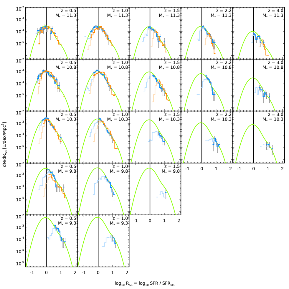
In Fig. 17 we show the distributions of “starburstiness” , defined as the ratio between the actual of each galaxy and , the they would have if they were exactly following the main sequence defined in Eq. 9. We analyze these distributions in the same bins that were used for stacking, to make the comparison simpler. Since the CANDELS fields have a relatively similar depth, we group them together into a single distribution (blue curve), and following Rodighiero et al. (2011) we keep the COSMOS UltraVISTA sources apart (orange curve) where the catalog is mass-complete.
As was the case for the stellar mass functions discussed in section 2.7, these distributions are affected by completeness issues. To correct this, we use a procedure very similar to that used for the mass functions. We assume that the total of a galaxy at a given redshift is well modeled from the rest-frame monochromatic luminosity in each Herschel band by a power law plus a Gaussian scatter in logarithmic space. In each bin of redshift and stellar mass, we select galaxies that are detected in at least three Herschel bands, fit this power law and measure the dispersion as in Fig. 2. In this case, this dispersion is mainly due to differences in dust temperature, and is found to be minimal at the peak of the FIR emission (see Fig. 9). Then, for each Herschel band, in each redshift and mass bin, we then generate a mock population of galaxies with uniform redshift and mass distribution within the bin and attribute a starburstiness with uniform probability to each mock galaxy. We multiply this starburstiness by the of the galaxy computed from its redshift and mass, subtract the average observed in this bin (we assume no scatter in for simplicity), convert the remaining into , and finally the into monochromatic luminosity in the considered Herschel band, adding a random logarithmic scatter whose amplitude is given by the dispersion measured earlier. The completeness is then given as the fraction of mock galaxies with simulated monochromatic luminosity larger than the limiting luminosity at the corresponding redshift.
Since we include in our sample all sources provided that they are detected in at least one Herschel band, we then take the maximum completeness among all bands. In Fig. 17, raw incomplete counts are shown as light curves in the background, and corrected counts are shown as darker lines. Error bars indicate Poisson noise and for clarity are only shown for the CANDELS counts.
In all fields, the low counts at come from MIPS derived s. Since the MIPS imaging in COSMOS UltraVISTA is only half as deep as the deepest CANDELS fields (see section 2.3 and Table 1), the two curves probe almost similar ranges of . At (i.e., starting from the bin at ) MIPS is not used any more, and the difference in depth of the Herschel surveys becomes quite obvious. Reassuringly, we see very good agreement between the two data sets where they overlap.
4.6.3 Evolution of the fraction of starbursts
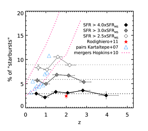
From these distributions, we can derive interesting statistical properties of our star-forming galaxy sample. In particular, Rodighiero et al. (2011) reported that only to of the galaxies in their sample were in a “starburst” mode, with an increased by more than a factor (or ) compared to the main sequence (i.e., ). Using our data set, we are able to measure this fraction at different redshifts and look for an evolution of this population. To do so, we select in each redshift bin all star-forming galaxies more massive than (this mass threshold is chosen to avoid completeness issues), and compute the fraction of objects for which the observed is at least a factor above the main sequence. Following Rodighiero et al. (2011), we choose . However, to make sure that our results are not affected by this somewhat abritrary choice, we also do this analysis with and . By lowering this threshold, the number of objects increases and the statistics become more robust, at the price of having a higher number of nonstarburst contaminants scattering from the main sequence. We could have overcome this problem by fitting the observed counts, decomposing the total distribution as coming from two populations: a main-sequence component and a starburst component, as was done in Sargent et al. (2012). While such a deconvolution provides a more physical definition of a “starburst”, it is also dependent on the model one choses to describe the starburst population. Also, except in a few low redshift bins, our data do not probe a wide enough range to be able to robustly perform this decomposition. We therefore choose this simpler approach of a fixed threshold for now, and will come back to the decomposition later. The results are presented in Fig. 18. Between and and for , we measure a roughly constant value ranging between and , and no clear trend with redshift emerges. We discuss the implication of this fact in section 5.2.
4.6.4 Quantifying the contribution of starbursts to the total budget
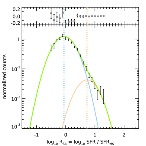
We now normalize the counts by the integral of the stellar mass function in all bins and, supported by our findings on the constant width of the main sequence (Fig. 12) and on a constant starburst fraction (Fig. 18), we assume that the distribution does not vary. With this same assumption of an unvarying distribution, Sargent et al. (2012) managed to reconstruct the IR luminosity function at various redshifts. With the increased statistics, we are now able to perform a two-component decomposition of the whole distribution. We thus fit all the counts simultaneously with a double log-normal distribution following Sargent et al. (2012). The chosen parametrization for the fit is
| (10) |
where and are the widths of the main sequence and starburst distributions, respectively, is the fraction of starbursts, and is the median multiplicative boost of starburst galaxies. We also introduce as the fraction of star-forming galaxies that are neither “main sequence” nor “starburst” galaxies (e.g., “green valley” galaxies), and the median of main-sequence galaxies. By construction, the latter two parameters should be close to and , respectively, but we allow them to vary to check for the consistency between the detections and the stacks.
The result is shown in Fig. 19. Leaving all parameters free, the fit of the starburst population is highly uncertain, so we decided to fix , and fit the logarithm of the counts. We obtain , , , , and .
These numbers depend heavily on the chosen parametrization of the starburst population. For example, not imposing would change the values of considerably, hence the measured values should be used with caution. The integrated contribution of the starburst population is however well constrained (Sargent et al., 2012). Taking these numbers at face value, we reach a similar conclusion as Rodighiero et al. (2011) and Sargent et al. (2012), i.e., that starbursts are rare and happen in only about of galaxies at a given instant. However, they form stars on average times faster than their main-sequence counterparts, and thus contribute to of the budget. It is worth noting that the bimodality, if any, is not clearly apparent in our data, and the high counts can also be fit with a single power law (with a slope close to ). While our goal is not to demonstrate the validity of this bimodal decomposition, we want to stress that the absence of a “gap” in the distribution between the peaks of the two components does not rule out the bimodal hypothesis.
The main-sequence distribution, on the other hand, is very well constrained and both its average and the measured are in agreement with the stacked value. The fact that is close to zero means that we are able to recover essentially all the star-forming galaxies with this model. More precisely, if there is another population of star-forming galaxies, we can say with probability that it can only make up for less than of the counts.
Last but not least, the accuracy of the fit in all the bins (as shown in Fig. 17) confirms the validity of our hypothesis of a universal distribution.
5 Discussion
5.1 Connection of the main-sequence dispersion with feedback processes
The nonevolution of the main-sequence dispersion, as described in section 4.4, is intriguing. Indeed, this dispersion can originate from several completely different processes. On the one hand, the scatter within the star formation history (SFH) of individual galaxies, i.e., bursts of star formation due to minor or major merging and feedback from AGNs or supernova winds, will naturally broaden the distribution of . On the other hand, the scatter may also be due to one or more missing variables, such as age, metallicity, geometry, or environment. For example, Salmi et al. (2012) found, using based s at , that the dispersion of the main sequence could artificially be reduced to about by introducing the rest-frame color as well as -band clumpiness as extra variables. This also shows that most of the observed scatter of the main sequence is physical and not due to measurement errors.
Hopkins et al. (2014) have computed the expected scatter of SFH from a set of numerical simulations, and found it to be a strong function of halo mass, and thus of stellar mass. Performing abundance matching using their – relation, one finds that they predict a variation of the (averaged over , hence comparable to the timescale of our FIR tracer) of about at , rising up to as stellar mass decreases down to . They also find that this evolution is coming predominantly from the rising importance of stellar feedback, and not from merging or global gravitational instabilities. Intuitively, the smaller the galaxy, the more sensitive it is to the impact of stellar winds and super novae, since the characteristic length scale over which these phenomena tend to heat and blow away the gas is more or less constant. Since there are other components that add up to the total scatter in (age, environment, metallicity, etc.), this prediction should be considered as a lower limit.
The predicted values of Hopkins et al. (2014) are shown as the purple line in Fig. 12. The dependence of their prediction on stellar mass is clear, yet we seem to measure a constant value. Even though there are other sources of scatter at play, it would be a strange conspiracy for them to exactly counterbalance the evolution of the scatter within the SFH to maintain a constant main-sequence scatter (see however Sparre et al., 2014). Our interpretation is thus the following.
Stellar feedback is a necessary ingredient in numerical simulations. Without it, galaxies would consume their gas too efficiently, and with the amount of infalling gas they receive from the inter-galactic medium, they would end up today with extremely high stellar masses that are not observed. The real strength of the stellar feedback is poorly constrained, so it is usually considered as a free parameter and fine-tuned to reproduce the local stellar mass density. However, our observations show that it cannot be arbitrarily high. Other processes can be considered to either decrease the star formation efficiency of galaxies, or reduce the amount of infalling gas they receive (e.g., Gabor & Bournaud, 2014).
5.2 Connection between starbursts and mergers
We have shown in section 4.6 that the starburst population is not evolving, both in relative numbers and excess with respect to the main sequence. This is intriguing in many aspects. Both observations (Le Fèvre et al., 2000; Kartaltepe et al., 2007; Lotz et al., 2011, and references therein) and numerical simulations (e.g., Somerville et al., 2008; Hopkins et al., 2010a) predict an increase of the major merger rate with increasing redshift, typically proportional to . Although the slope of the evolution of the merger fraction is quite uncertain (see discussion in Kampczyk et al., 2007), it is always found to be positive, ranging from up to . For example, Kartaltepe et al. (2007) analyzed the fraction of close pairs from to , and found . Their value of is comparable to our observed starburst fraction with , however extrapolating this relation to would predict a pair fraction of about ( if we consider instead the numerical simulation of Hopkins et al., 2010a). If all or a constant fraction of those pairs do lead to gas-rich major mergers, this would have a huge impact on the number of starburst, at odds with our observations.
On the other hand, Perret et al. (2014) ran several numerical simulations of mergers of clumpy galaxies, and found little to no impact of the merger on star formation when compared to isolated galaxies. Their point is that by star formation is already fairly active in isolated galaxies and actually close to a saturation point due to feedback processes. When the merger happens, it therefore cannot increase the total by a large amount because star formation is already at its maximum. So even if mergers were more frequent in the past, they were also less efficient at triggering bursts of star formation, and this could explain why we are not seeing a huge increase in the number of starburst galaxies. This goes in the same direction as the results of Hopkins et al. (2010b) who found in their simulations that merger-driven bursts contribute to the same fraction (–) of the IR luminosity function at all redshifts, but it does not explain why the fraction of such bursts remains constant over time.
Although the most extreme starburst events are unambiguously associated with major mergers in the local Universe (e.g., Armus et al., 1987), another interpretation of our results is that the situation may be different at earlier epochs, and that some other phenomena may be responsible for such bursts of star formation, such as large scale dynamical instabilities (e.g., Dekel et al., 2009b).
6 Conclusions
We have put together a catalog of star-forming galaxies that is mass-complete above and extends up to , using the deep UV to NIR observations in the CANDELS fields. By stacking the Herschel images at the positions of these galaxies, using bins of mass and redshift, we measured their average star formation rates in a dust-unbiased way. We then derived a new technique called “scatter stacking” to measure the scatter in around the average stacked value. We also analyzed sources individually detected on the Herschel images to study the distribution in more detail over a more limited range of redshift and stellar mass.
We observe a continuously rising up to , with no clear sign of a saturation or plateau at the highest redshifts. Previous observations of this type of saturation are mostly based on LBG samples that lack observations in the FIR to reliably constrain the dust extinction. Earlier results are likely due to a combination of selection effects and biases in the dust extinction correction. It is therefore mandatory to have mass-complete samples and rest-frame MIR or FIR data to provide reliable constraints on the star formation activity of actively star-forming galaxies.
We find that the slope of the – relation is close to unity, except for high mass galaxies (), where the slope is shallower. Furthermore, the high mass slope is evolving from at high redshifts down to almost at . One possible explanation is the increasing contribution of the bulge to the stellar mass of these galaxies, while the star formation rates come mostly from the disk (Abramson et al., 2014).
At fixed mass and redshift, the scatter around the average appears to be constant and close to from to , with no clear redshift dependence. We therefore confirm the existence of the “main sequence” of star-forming galaxies over a large range of mass and redshift with a robust star formation rate tracer. We show that at least of present day stars were formed in main-sequence galaxies. Consequently, whatever physical process produces the main sequence is the dominant mode of stellar growth in galaxies.
The nonevolution of the scatter with mass can be connected to the expected strength of stellar feedback. State-of-the-art numerical simulations indeed predict that stellar feedback generates additional scatter in the star formation histories of galaxies, a scatter whose amplitude is strongly anticorrelated with halo mass and thus galaxy mass. Our observations provide useful constraints for numerical simulations where stellar feedback is often used as an efficient star formation regulator. We show here that it cannot be arbitrarily high.
Refining the above analysis with individual Herschel detections, we look for starburst galaxies whose s are systematically larger than those of main-sequence galaxies. In agreement with Sargent et al. (2012) and extending their analysis to higher redshifts and more complete samples, we find that the fraction of these starburst galaxies does not evolve with time. This questions the usual interpretation of starburst as the consequence of triggering by major mergers. Several studies, both of simulations and observations, indeed show that the fraction of mergers was substantially higher in the past. An alternative explanation is that mergers may be less efficient at creating bursts of star formation within high redshift galaxies.
We have pushed Herschel as far as possible to study the main sequence of star-forming galaxies, but it is still necessary to dig deeper than that, i.e., probing higher redshifts or lower stellar masses. Most of what we know at present about the high redshift Universe () comes from rest-frame UV-based studies, and we have shown here that dust extinction plays an important role even at these redshifts. Therefore it will be necessary to explore these epochs of the Universe with an independent and more robust tracer to confirm the pioneering results obtained with the UV light alone. Probing lower stellar masses will also be an important challenge since, owing to their small sizes, low mass () galaxies are probably most sensitive to smaller scale physics, e.g., stellar or AGN feedback.
Valuable insights already come from the study of lensed galaxies. This technique allows us to observe galaxies about an order of magnitude fainter than the nominal instrument depths, either by chance in blank fields (e.g., the Herschel ATLAS, Eales et al., 2010), or by explicitly targeting large galaxy clusters (e.g., the Herschel Lensing Survey, Egami et al., 2010). Studying these regimes on statistically relevant samples and with a dust-unbiased tracer will only be possible with a new generation of instruments. The most promising candidate available today for the high redshift Universe is certainly the Atacama Large Millimeter/submillimeter Array (ALMA), and interesting science is already on its way. In particular, we are now waiting for the completion of Cycle 2 observations targeting a mass-complete sample of star-forming galaxies down to . With only a few minutes of on-source integration, these data will allow us to probe s about five times lower than those available with the deepest Herschel surveys. As for the low mass galaxies, substantial progress is likely to happen in a few years thanks to the exceptional MIR capabilities of the James Webb Space Telescope (JWST).
Acknowledgements.
The authors want to thank the anonymous referee for his/her comments that clearly improved the consistency and overall quality of this paper. CS and DE are grateful to F. Bournaud for the enlightening discussions that motivated certain aspects of this paper. SJ acknowledges support from the EU through grant ERC-StG-257720. Most of the numerical analysis conducted in this work have been performed using phy++, a free and open source C++ library for fast and robust numerical astrophysics (http://cschreib.github.io/phypp/). This work is based on observations taken by the CANDELS Multi-Cycle Treasury Program with the NASA/ESA HST, which is operated by the Association of Universities for Research in Astronomy, Inc., under NASA contract NAS5-26555. This research was supported by the French Agence Nationale de la Recherche (ANR) project ANR-09-BLAN-0224 and by the European Commission through the FP7 SPACE project ASTRODEEP (Ref.No: 312725).References
- Abramson et al. (2014) Abramson, L. E., Kelson, D. D., Dressler, A., et al. 2014, ApJ, 785, L36
- Armus et al. (1987) Armus, L., Heckman, T., & Miley, G. 1987, AJ, 94, 831
- Baldry et al. (2004) Baldry, I. K., Glazebrook, K., Brinkmann, J., et al. 2004, ApJ, 600, 681
- Bell et al. (2003) Bell, E. F., McIntosh, D. H., Katz, N., & Weinberg, M. D. 2003, ApJS, 149, 289
- Benítez (2000) Benítez, N. 2000, ApJ, 536, 571
- Bertin & Arnouts (1996) Bertin, E. & Arnouts, S. 1996, A&AS, 117, 393
- Béthermin et al. (2010) Béthermin, M., Dole, H., Cousin, M., & Bavouzet, N. 2010, A&A, 516, 43
- Béthermin et al. (2012) Béthermin, M., Le Floc’h, E., Ilbert, O., et al. 2012, A&A, 542, 58
- Bouché et al. (2010) Bouché, N., Dekel, A., Genzel, R., et al. 2010, ApJ, 718, 1001
- Bouwens et al. (2012) Bouwens, R. J., Illingworth, G. D., Oesch, P. A., et al. 2012, ApJ, 754, 83
- Brammer et al. (2008) Brammer, G. B., van Dokkum, P. G., & Coppi, P. 2008, ApJ, 686, 1503
- Brammer et al. (2011) Brammer, G. B., Whitaker, K. E., van Dokkum, P. G., et al. 2011, ApJ, 739, 24
- Bressan et al. (1993) Bressan, A., Fagotto, F., Bertelli, G., & Chiosi, C. 1993, A&AS, 100, 647
- Brinchmann et al. (2004) Brinchmann, J., Charlot, S., White, S. D. M., et al. 2004, MNRAS, 351, 1151
- Bruzual & Charlot (2003) Bruzual, G. & Charlot, S. 2003, MNRAS, 344, 1000
- Buat et al. (2005) Buat, V., Iglesias-Páramo, J., Seibert, M., et al. 2005, ApJ, 619, L51
- Calzetti et al. (2000) Calzetti, D., Armus, L., Bohlin, R. C., et al. 2000, ApJ, 533, 682
- Calzetti et al. (1994) Calzetti, D., Kinney, A. L., & Storchi-Bergmann, T. 1994, ApJ, 429, 582
- Cardamone et al. (2010) Cardamone, C. N., Urry, C. M., Schawinski, K., et al. 2010, ApJ, 721, L38
- Castellano et al. (2014) Castellano, M., Sommariva, V., Fontana, A., et al. 2014, A&A, 566, 19
- Chary & Elbaz (2001) Chary, R. & Elbaz, D. 2001, ApJ, 556, 562
- Chary & Pope (2010) Chary, R. & Pope, A. 2010, ArXiv e-prints, 1003.1731
- Cole et al. (2001) Cole, S., Norberg, P., Baugh, C. M., et al. 2001, MNRAS, 326, 255
- Conselice et al. (2003) Conselice, C. J., Bershady, M. A., Dickinson, M., & Papovich, C. 2003, AJ, 126, 1183
- Daddi et al. (2010) Daddi, E., Bournaud, F., Walter, F., et al. 2010, ApJ, 713, 686
- Daddi et al. (2004) Daddi, E., Cimatti, A., Renzini, A., et al. 2004, ApJ, 617, 746
- Daddi et al. (2009) Daddi, E., Dannerbauer, H., Stern, D., et al. 2009, ApJ, 694, 1517
- Daddi et al. (2007) Daddi, E., Dickinson, M., Morrison, G., et al. 2007, ApJ, 670, 156
- Davé et al. (2011) Davé, R., Finlator, K., & Oppenheimer, B. D. 2011, MNRAS, 416, 1354
- Dekel et al. (2009a) Dekel, A., Birnboim, Y., Engel, G., et al. 2009a, Nature, 457, 451
- Dekel et al. (2009b) Dekel, A., Sari, R., & Ceverino, D. 2009b, ApJ, 703, 785
- Díaz-Santos et al. (2013) Díaz-Santos, T., Armus, L., Charmandaris, V., et al. 2013, ApJ, 774, 68
- Dole et al. (2006) Dole, H., Lagache, G., Puget, J., et al. 2006, A&A, 451, 417
- Eales et al. (2010) Eales, S., Dunne, L., Clements, D., et al. 2010, PASP, 122, 499
- Egami et al. (2010) Egami, E., Rex, M., Rawle, T. D., et al. 2010, A&A, 518, L12
- Elbaz et al. (2007) Elbaz, D., Daddi, E., Le Borgne, D., et al. 2007, A&A, 468, 33
- Elbaz et al. (2011) Elbaz, D., Dickinson, M., Hwang, H. S., et al. 2011, A&A, 533, 119
- Fadda et al. (2010) Fadda, D., Yan, L., Lagache, G., et al. 2010, ApJ, 719, 425
- Gabor & Bournaud (2014) Gabor, J. M. & Bournaud, F. 2014, MNRAS, 441, 1615
- Galametz et al. (2013) Galametz, A., Grazian, A., Fontana, A., et al. 2013, ApJS, 206, 10
- Geach et al. (2011) Geach, J. E., Smail, I., Moran, S. M., et al. 2011, ApJ, 730, L19
- Genzel et al. (2014) Genzel, R., Tacconi, L. J., Lutz, D., et al. 2014, ArXiv e-prints, 1409.1171
- Gladders et al. (2013) Gladders, M. D., Oemler, A., Dressler, A., et al. 2013, ApJ, 770, 64
- Goldader et al. (2002) Goldader, J. D., Meurer, G., Heckman, T. M., et al. 2002, ApJ, 568, 651
- González et al. (2014) González, V., Bouwens, R., Illingworth, G., et al. 2014, ApJ, 781, 34
- Griffin et al. (2010) Griffin, M. J., Abergel, A., Abreu, A., et al. 2010, A&A, 518, L3
- Grogin et al. (2011) Grogin, N. A., Kocevski, D. D., Faber, S. M., et al. 2011, ApJS, 197, 35
- Guo et al. (2013) Guo, K., Zheng, X. Z., & Fu, H. 2013, ApJ, 778, 23
- Hatziminaoglou et al. (2010) Hatziminaoglou, E., Omont, A., Stevens, J. A., et al. 2010, A&A, 518, L33
- Heinis et al. (2013) Heinis, S., Buat, V., Béthermin, M., et al. 2013, MNRAS, 429, 1113
- Heinis et al. (2014) Heinis, S., Buat, V., Béthermin, M., et al. 2014, MNRAS, 437, 1268
- Hopkins et al. (2010a) Hopkins, P. F., Bundy, K., Croton, D., et al. 2010a, ApJ, 715, 202
- Hopkins et al. (2014) Hopkins, P. F., Kereš, D., Oñorbe, J., et al. 2014, MNRAS, 445, 581
- Hopkins et al. (2010b) Hopkins, P. F., Younger, J. D., Hayward, C. C., Narayanan, D., & Hernquist, L. 2010b, MNRAS, 402, 1693
- Ilbert et al. (2013) Ilbert, O., McCracken, H. J., Le Fèvre, O., et al. 2013, A&A, 556, 55
- Juneau et al. (2013) Juneau, S., Dickinson, M., Bournaud, F., et al. 2013, ApJ, 764, 176
- Kampczyk et al. (2007) Kampczyk, P., Lilly, S. J., Carollo, C. M., et al. 2007, ApJS, 172, 329
- Kartaltepe et al. (2007) Kartaltepe, J. S., Sanders, D. B., Scoville, N. Z., et al. 2007, ApJS, 172, 320
- Kauffmann et al. (2003) Kauffmann, G., Heckman, T. M., Tremonti, C., et al. 2003, MNRAS, 346, 1055
- Kennicutt (1998) Kennicutt, Robert C., J. 1998, ARA&A, 36, 189
- Koekemoer et al. (2011) Koekemoer, A. M., Faber, S. M., Ferguson, H. C., et al. 2011, ApJS, 197, 36
- Koyama et al. (2013) Koyama, Y., Smail, I., Kurk, J., et al. 2013, MNRAS, 434, 423
- Kriek et al. (2009) Kriek, M., van Dokkum, P. G., Labbé, I., et al. 2009, ApJ, 700, 221
- Kurczynski & Gawiser (2010) Kurczynski, P. & Gawiser, E. 2010, AJ, 139, 1592
- Laidler et al. (2007) Laidler, V. G., Papovich, C., Grogin, N. A., et al. 2007, PASP, 119, 1325
- Le Fèvre et al. (2000) Le Fèvre, O., Abraham, R., Lilly, S. J., et al. 2000, MNRAS, 311, 565
- Le Floc’h et al. (2009) Le Floc’h, E., Aussel, H., Ilbert, O., et al. 2009, ApJ, 703, 222
- Le Floc’h et al. (2005) Le Floc’h, E., Papovich, C., Dole, H., et al. 2005, ApJ, 632, 169
- Lee et al. (2013) Lee, N., Sanders, D. B., Casey, C. M., et al. 2013, ApJ, 778, 131
- Leroy et al. (2008) Leroy, A. K., Walter, F., Brinks, E., et al. 2008, AJ, 136, 2782
- Lilly et al. (2013) Lilly, S. J., Carollo, C. M., Pipino, A., Renzini, A., & Peng, Y. 2013, ApJ, 772, 119
- Lilly et al. (1996) Lilly, S. J., Le Fevre, O., Hammer, F., & Crampton, D. 1996, ApJ, 460, L1
- Lotz et al. (2011) Lotz, J. M., Jonsson, P., Cox, T. J., et al. 2011, ApJ, 742, 103
- Lutz et al. (2011) Lutz, D., Poglitsch, A., Altieri, B., et al. 2011, A&A, 532, 90
- Madau & Dickinson (2014) Madau, P. & Dickinson, M. 2014, ArXiv e-prints, 1403.0007
- Madau et al. (1996) Madau, P., Ferguson, H. C., Dickinson, M. E., et al. 1996, MNRAS, 283, 1388
- Madau et al. (1998) Madau, P., Pozzetti, L., & Dickinson, M. 1998, ApJ, 498, 106
- Magdis et al. (2012) Magdis, G. E., Daddi, E., Béthermin, M., et al. 2012, ApJ, 760, 6
- Magdis et al. (2010) Magdis, G. E., Elbaz, D., Daddi, E., et al. 2010, ApJ, 714, 1740
- Magnelli et al. (2009) Magnelli, B., Elbaz, D., Chary, R. R., et al. 2009, A&A, 496, 57
- Magnelli et al. (2014) Magnelli, B., Lutz, D., Saintonge, A., et al. 2014, A&A, 561, 86
- Magnelli et al. (2013) Magnelli, B., Popesso, P., Berta, S., et al. 2013, A&A, 553, 132
- Marsden et al. (2009) Marsden, G., Ade, P. A. R., Bock, J. J., et al. 2009, ApJ, 707, 1729
- McCracken et al. (2012) McCracken, H. J., Milvang-Jensen, B., Dunlop, J., et al. 2012, A&A, 544, 156
- Meurer et al. (1999) Meurer, G. R., Heckman, T. M., & Calzetti, D. 1999, ApJ, 521, 64
- Mullaney et al. (2011) Mullaney, J. R., Alexander, D. M., Goulding, A. D., & Hickox, R. C. 2011, MNRAS, 414, 1082
- Mullaney et al. (2012) Mullaney, J. R., Pannella, M., Daddi, E., et al. 2012, MNRAS, 419, 95
- Murata et al. (2014) Murata, K. L., Matsuhara, H., & Inami, H. 2014
- Muzzin et al. (2013a) Muzzin, A., Marchesini, D., Stefanon, M., et al. 2013a, ApJ, 777, 18
- Muzzin et al. (2013b) Muzzin, A., Marchesini, D., Stefanon, M., et al. 2013b, ApJS, 206, 8
- Nguyen et al. (2010) Nguyen, H. T., Schulz, B., Levenson, L., et al. 2010, A&A, 518, L5
- Noeske et al. (2007) Noeske, K. G., Weiner, B. J., Faber, S. M., et al. 2007, ApJ, 660, L43
- Nordon et al. (2012) Nordon, R., Lutz, D., Genzel, R., et al. 2012, ApJ, 745, 182
- Oliver et al. (2012) Oliver, S. J., Bock, J., Altieri, B., et al. 2012, MNRAS, 424, 1614
- Oteo et al. (2013) Oteo, I., Cepa, J., Bongiovanni, A., et al. 2013, A&A, 554, L3
- Overzier et al. (2011) Overzier, R. A., Heckman, T. M., Wang, J., et al. 2011, ApJ, 726, L7
- Pannella et al. (2009) Pannella, M., Carilli, C. L., Daddi, E., et al. 2009, ApJ, 698, L116
- Pannella et al. (2014) Pannella, M., Elbaz, D., Daddi, E., et al. 2014, ArXiv e-prints, 1407.5072
- Patton et al. (1997) Patton, D. R., Pritchet, C. J., Yee, H. K. C., Ellingson, E., & Carlberg, R. G. 1997, ApJ, 475, 29
- Peng et al. (2010) Peng, Y.-j., Lilly, S. J., Kovač, K., et al. 2010, ApJ, 721, 193
- Penner et al. (2012) Penner, K., Dickinson, M., Pope, A., et al. 2012, ApJ, 759, 28
- Perret et al. (2014) Perret, V., Renaud, F., Epinat, B., et al. 2014, A&A, 562, 1
- Pilbratt et al. (2010) Pilbratt, G. L., Riedinger, J. R., Passvogel, T., et al. 2010, A&A, 518, L1
- Poglitsch et al. (2010) Poglitsch, A., Waelkens, C., Geis, N., et al. 2010, A&A, 518, L2
- Pope et al. (2008) Pope, A., Chary, R., Alexander, D. M., et al. 2008, ApJ, 675, 1171
- Prantzos & Silk (1998) Prantzos, N. & Silk, J. 1998, ApJ, 507, 229
- Reddy et al. (2012) Reddy, N. A., Pettini, M., Steidel, C. C., et al. 2012, ApJ, 754, 25
- Rieke et al. (2004) Rieke, G. H., Young, E. T., Engelbracht, C. W., et al. 2004, ApJS, 154, 25
- Rodighiero et al. (2010) Rodighiero, G., Cimatti, A., Gruppioni, C., et al. 2010, A&A, 518, L25
- Rodighiero et al. (2011) Rodighiero, G., Daddi, E., Baronchelli, I., et al. 2011, ApJ, 739, L40
- Rodighiero et al. (2014) Rodighiero, G., Renzini, A., Daddi, E., et al. 2014, MNRAS, 443, 19
- Rosario et al. (2013) Rosario, D. J., Santini, P., Lutz, D., et al. 2013, ApJ, 771, 63
- Rujopakarn et al. (2011) Rujopakarn, W., Rieke, G. H., Eisenstein, D. J., & Juneau, S. 2011, ApJ, 726, 93
- Saintonge et al. (2013) Saintonge, A., Lutz, D., Genzel, R., et al. 2013, ApJ, 778, 2
- Salim et al. (2009) Salim, S., Dickinson, M., Michael Rich, R., et al. 2009, ApJ, 700, 161
- Salmi et al. (2012) Salmi, F., Daddi, E., Elbaz, D., et al. 2012, ApJ, 754, L14
- Salmon et al. (2014) Salmon, B., Papovich, C., Finkelstein, S. L., et al. 2014, ArXiv e-prints, 1407.6012
- Salpeter (1955) Salpeter, E. E. 1955, ApJ, 121, 161
- Salvato et al. (2011) Salvato, M., Ilbert, O., Hasinger, G., et al. 2011, ApJ, 742, 61
- Sanders & Mirabel (1996) Sanders, D. B. & Mirabel, I. F. 1996, ARA&A, 34, 749
- Sanders et al. (2007) Sanders, D. B., Salvato, M., Aussel, H., et al. 2007, ApJS, 172, 86
- Santini et al. (2009) Santini, P., Fontana, A., Grazian, A., et al. 2009, A&A, 504, 751
- Santini et al. (2014) Santini, P., Maiolino, R., Magnelli, B., et al. 2014, A&A, 562, 30
- Santini et al. (2012) Santini, P., Rosario, D. J., Shao, L., et al. 2012, A&A, 540, 109
- Sargent et al. (2012) Sargent, M. T., Béthermin, M., Daddi, E., & Elbaz, D. 2012, ApJ, 747, L31
- Somerville et al. (2008) Somerville, R. S., Hopkins, P. F., Cox, T. J., Robertson, B. E., & Hernquist, L. 2008, MNRAS, 391, 481
- Sparre et al. (2014) Sparre, M., Hayward, C. C., Springel, V., et al. 2014, ArXiv e-prints, 1409.0009
- Speagle et al. (2014) Speagle, J. S., Steinhardt, C. L., Capak, P. L., & Silverman, J. D. 2014, ApJS, 214, 15
- Stark et al. (2009) Stark, D. P., Ellis, R. S., Bunker, A., et al. 2009, ApJ, 697, 1493
- Stark et al. (2013) Stark, D. P., Schenker, M. A., Ellis, R., et al. 2013, ApJ, 763, 129
- Steidel et al. (1999) Steidel, C. C., Adelberger, K. L., Giavalisco, M., Dickinson, M., & Pettini, M. 1999, ApJ, 519, 1
- Steinhardt et al. (2014) Steinhardt, C. L., Speagle, J. S., Capak, P., et al. 2014, ApJ, 791, L25
- Strazzullo et al. (2013) Strazzullo, V., Gobat, R., Daddi, E., et al. 2013, ApJ, 772, 118
- Tacconi et al. (2010) Tacconi, L. J., Genzel, R., Neri, R., et al. 2010, Nature, 463, 781
- Viero et al. (2013) Viero, M. P., Moncelsi, L., Quadri, R. F., et al. 2013, ApJ, 779, 32
- Wang et al. (2010) Wang, W., Cowie, L. L., Barger, A. J., Keenan, R. C., & Ting, H. 2010, ApJS, 187, 251
- Werner et al. (2004) Werner, M. W., Roellig, T. L., Low, F. J., et al. 2004, ApJS, 154, 1
- Whitaker et al. (2014) Whitaker, K. E., Franx, M., Leja, J., et al. 2014, ArXiv e-prints, 1407.1843
- Whitaker et al. (2011) Whitaker, K. E., Labbé, I., van Dokkum, P. G., et al. 2011, ApJ, 735, 86
- Whitaker et al. (2012) Whitaker, K. E., van Dokkum, P. G., Brammer, G., & Franx, M. 2012, ApJ, 754, L29
- White et al. (2007) White, R. L., Helfand, D. J., Becker, R. H., Glikman, E., & de Vries, W. 2007, ApJ, 654, 99
- Williams et al. (2009) Williams, R. J., Quadri, R. F., Franx, M., van Dokkum, P., & Labbé, I. 2009, ApJ, 691, 1879
- Wuyts et al. (2011) Wuyts, S., Förster Schreiber, N. M., Lutz, D., et al. 2011, ApJ, 738, 106
- Wuyts et al. (2007) Wuyts, S., Labbé, I., Franx, M., et al. 2007, ApJ, 655, 51
Appendix A The selection
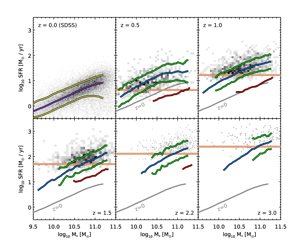
To further test the reliability of the selection technique, we have separately stacked the galaxies classified as quiescent. The result is presented in Fig. 20. On this plot we show what the location of the quiescent galaxies would be on the – plane assuming that all their IR luminosity is coming from star formation. This is certainly wrong because in these massive galaxies dust is mostly heated by old stars, so the we derive is actually an upper limit on the true star formation activity of these galaxies. However, even with this naive assumption, the derived s are an order of magnitude lower than that of the star-forming sample. We also observe that the effective dust temperature, inferred from the wavelength at which the FIR emission peaks, is lower and this is expected if dust is indeed mainly heated by less massive stars.
Appendix B Tests of our methods on simulated images
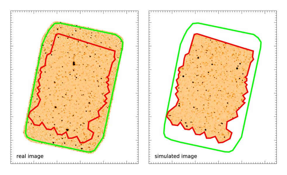
To test all of these procedures, we build a set of simulated images. We design these to be as close as possible to the real images in a statistical sense, i.e., the same photometric and confusion noise, and the same number counts.
To do so, we start from our observed -band catalogs, knowing redshifts and stellar masses for all the galaxies. Using our results from stacking Herschel images, we can attribute an to each of these galaxies. We then add a random amount of star formation, following a log-normal distribution of dispersion . We also put of our sources in starburst mode, where their is increased by . Next, we assign an FIR SED to each galaxy following the observed trends with redshift (no mass dependence) and excess (Magnelli et al. 2014). Starburst galaxies are also given warmer SEDs.
From these simulated source catalogs, we generate a list of fluxes in all Herschel bands. Given noise maps (either modeled from RMS maps assuming Gaussian noise, or constructed from the difference between observing blocks), we build simulated images by placing each source as a PSF centered on its sky position, with a Gaussian uncertainty of and a maximum offset of . We randomly reposition the sources inside the fields using uniform distributions in right ascension and declination, to probe multiple realizations of confusion. These simulated images have pixel distribution, or plots, very close to the observed images, and are thus good tools to study our methods. An example is shown in Fig. 21 for the GOODS–South field at .
We produce sets of simulated catalogs and images, each with a different realization of photometric noise, confusion noise and . We then run our full stacking procedure on each, using the same setup as for the real images (i.e., using the same redshift and mass bins), to test the reliability of our flux extraction and the accuracy of the reported errors.
B.1 Mean and median stacked fluxes
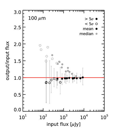
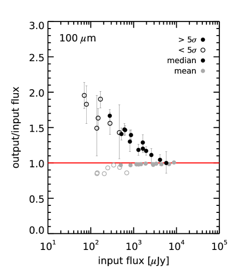
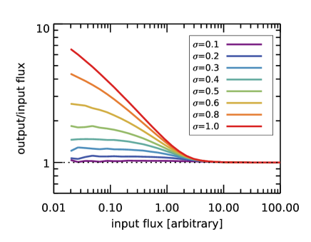
For each of the realizations we compare the measured flux densities using both mean and median stacking to the expected mean and median flux densities, respectively. The results are shown in Fig. 22 for the PACS band. The other bands show similar behavior.
Although less noisy, median fluxes are biased toward higher values (at most by a factor here). This is because the median is not a linear operation, so it is not true in general that , where denotes the median. In particular, this means that if we compute the median of our noisy stacked image and subtract the median value of the noise, we do not exactly recover the median flux density. We will call this effect the noise bias in what follows. White et al. (2007) show that this bias arises when: 1) the signal to noise ratio of stacked sources is low; and 2) the distribution of flux is skewed toward either faint or bright sources. The latter is indeed true in our simulations, since we used a log-normal distribution for the . Correcting for this effect is not trivial, as it requires knowledge of the real flux distribution. Indeed, Fig. 23 shows the amplitude of this bias for different log-normal flux dispersions, the highest dispersions producing the highest biases. White et al. (2007) argue that the median stacked flux is still a useful quantity, since it is actually a good measure of the mean of the distribution, but this is only true in the limit of low signal to noise ratios. In their first example, a double normal distribution, the measured median reaches the true mean for , but correctly measures the true median for .
Of course these values depend on the distribution itself, as is shown in Fig. 23. In particular, for a log-normal distribution with scatter, the mean is reached for , and the median for . Theoretically, the difference between the mean and the median for a log-normal distribution is . In our simulations, the typical flux dispersion within a stacking bin is , which yields a factor , in agreement with the maximum observed bias.
| — | ||||||
| — | — | |||||
| — | — | — | — |
To see how this affects the measured in practice, we list in Table 4 the ratio of the median to mean measured in each stacked bin, as measured on the real images. We showed in section 4.4 that the dispersion in is about . Therefore, assuming a log-normal distribution, we would theoretically expect the ratio of the median to mean to be close to . It is, however, clear from Table 4 that this is not the case in practice: the median is usually (but not always) much closer to the mean than expected for a noiseless situation. Therefore, the median stacked fluxes are often not measuring the median fluxes or the mean fluxes, but something in between. Since correcting for this bias requires assumptions on the flux distribution, we prefer (when possible) to use the more noisy but unbiased mean fluxes for this study.
B.2 Clustering correction
| Method | |||||
|---|---|---|---|---|---|
| A | |||||
| B | |||||
| C |
These values were obtained by computing the ratio of measured mean stacked fluxes to the expected mean fluxes in simulated images using our flux extraction method (see section 3.2). Median stacked fluxes are affected the same way, after removing the noise bias described in Appendix B.1. We also show the th and th percentiles of the bias distribution. The methods are: A, using our own flux extraction procedure section 3.2; B, using the full PSF; and C, using only the central pixel.
Among our random realizations, the measured mean fluxes do not show any systematic bias. However these simulations do not take the flux boosting caused by source physical clustering into account, because we assigned random positions to the sources in our catalog. To test the effect of clustering, we regenerate a new set of simulations, this time using the real optical positions of the sources and only varying the photometric noise and the s of the sources.
If galaxies are significantly clustered in the image, then the measured fluxes will be boosted by the amount of light from clustered galaxies that falls inside the beam. Since the beam size here is almost a linear function of the wavelength, we expect SPIRE bands to be more affected than PACS bands. Since the same beam at different redshifts corresponds to different proper distances, low redshift measurements () should be less affected. However, because of the flatness of the relation between redshift and proper distance for , this should not have a strong impact for most of our sample. Indeed, we do not observe any significant trend with redshift in our simulations. No trend was found with stellar mass either, hence we averaged the clustering signal over all stacked bins for a given band, and report the average measured boost in Table 5 (“method A”) along with the th and th percentiles. Although we limited this analysis to fluxes measured at better than , the scatter in the measured bias is compatible with being only caused by uncertainties in flux extraction.
| — | ||||||
| — | ||||||
| — | — | — |
Although negligible in PACS, this effect can reach in SPIRE data. Here we correct for this bias by simply deboosting the real measured fluxes by the factors listed in Table 5, band by band. The net effect on the total measured is reported in Table 6.
By construction, these corrections are specific to our flux extraction method. By limiting the fitting area to pixels where the PSF relative amplitude is larger than , we absorb part of the large scale clustering into the background level. If we were to use the full PSF to measure the fluxes, we would measure a larger clustering signal (see section 3.2). We have re-extracted all the fluxes by fitting the full PSF, and we indeed measure larger biases. These are tabulated in Table 5 as “method B”. An alternative to PSF fitting that is less affected by clustering consists of setting the mean of the flux map to zero before stacking and then only using the central pixel of the stacked cutout (Béthermin et al. 2012). Because of clustering, the effective PSF of the stacked sources will be broadened, and using the real PSF to fit this effective PSF will result in some additional boosting. Therefore, by only using the central pixel, one can get rid of this effect. We show in Table 5 as “method C” how the figures change using this alternative method. Indeed the measured boosting is smaller than when using the full PSF, and is consistent with that reported by Béthermin et al. (2014, submitted), but our method is even less affected thanks to the use of a local background.
B.3 Error estimates
We now study the reliability of our error estimates on the stacked fluxes. We compute the difference between the observed and input flux for each realization, . We then compute the median , which is essentially the value plotted in Fig. 22, i.e., it is nonzero mostly for median stacked fluxes. We subtract this median difference from , and compute the scatter of the resulting quantity using median absolute deviation, i.e., . We show in Fig. 25 the histograms of for the mean and median stacked PACS fluxes in each stacked bin. By construction, these distributions are well described by a Gaussian of width unity (black curve).
We have two error estimates at our disposal. The first, , is obtained by measuring the RMS of the residual image (after the stacked fluxes have been fitted and subtracted), and multiplying this value by the PSF error factor (see Eq. 4). The second, , is obtained by bootstrapping, i.e., repeatedly stacking half of the parent sample and measuring the standard deviation of the resulting flux distribution (again, see section 3.2). Each of these method provides a different estimation of the error on the flux measurement, and we want to test their accuracy.
In Fig. 25, we show as red and blue lines the predicted error distribution according to and , respectively. When the predicted distribution is too narrow or too broad compared to the observed distribution (black curve), this means that the estimated error is respectively too low or too high.
For median stacked fluxes, it appears that is accurate in all cases. It tends to slightly overestimate the true error on some occasions, but not by a large amount. On the other hand, dramatically underestimates the error when the measured of stacked sources is high (or the number of stacked sources is low).
The situation for mean stacked fluxes is quite different. The behavior of is the same, but show the completely opposite trend, i.e., it underestimates the error at low signal to noise and high number of stacked sources. This may be caused by the fact that bootstrapping will almost always produce the same confusion noise, since it uses the same sources. The reason why this issue does not arise for median stacked fluxes might be because the median naturally filters out bright neighbors, hence reducing the impact of confusion noise.
The results are the same for the PACS and band. Therefore, keeping the maximum error between and ensures that one has an accurate error measurement in all cases for the PACS bands.
The SPIRE fluxes on the other hand show a substantially different behavior. We reproduce the same figures in Fig. 26, this time for the SPIRE band. Here, and except for the highest mass bin, the errors are systematically underestimated by a factor of , regardless of the estimator used. We therefore use this factor to correct all our measured SPIRE errors in these bins.
We believe this underestimation of the error is an effect of confusion noise. Indeed, it is clear when looking at the stacked maps at these wavelengths (e.g., Fig. 5) that there is a substantial amount of large scale noise coming from the contribution of the neighboring bright sources. The main issue with this noise is that it is spatially correlated. This violates one of the assumptions that were made when deriving the error estimation of Eq. 4, which may thus give wrong results. The reason why only the SPIRE bands are affected is because the noise budget here is (by design) completely dominated by confusion. This is clear from Fig. 24 (left): when putting little to no instrumental noise on the simulated maps, the total error on the flux measurements is completely dominated by the confusion noise (blue line), and it is only by adding instrumental noise of at least (i.e., ten times more than what is present in the real maps) that the image becomes noise dominated. By fitting
| (11) |
we obtain . This value depends on the model we used to generate the simulated fluxes, but it is in relatively good agreement with already published estimates from the literature (e.g., Nguyen et al. 2010, who predict ).
We then show in Fig. 24 (right) that the error underestimation in the SPIRE bands, here quantified by the ratio , goes away when the image is clearly noise dominated, meaning that this issue is indeed caused by confusion and the properties of the noise that it generates.