Three-dimensional simulations of core-collapse supernovae: from shock revival to shock breakout

We present three-dimensional hydrodynamic simulations of the evolution of core-collapse supernovae from blast-wave initiation by the neutrino-driven mechanism to shock breakout from the stellar surface, using an axis-free Yin-Yang grid and considering two 15 $M_{\odot}$ red supergiants (RSG) and two blue supergiants (BSG) of 15 $M_{\odot}$ and 20 $M_{\odot}$. We demonstrate that the metal-rich ejecta in homologous expansion still carry fingerprints of asymmetries at the beginning of the explosion, but the final metal distribution is massively affected by the detailed progenitor structure. The most extended and fastest metal fingers and clumps are correlated with the biggest and fastest-rising plumes of neutrino-heated matter, because these plumes most effectively seed the growth of Rayleigh-Taylor (RT) instabilities at the C+O/He and He/H composition-shell interfaces after the passage of the SN shock. The extent of radial mixing, global asymmetry of the metal-rich ejecta, RT-induced fragmentation of initial plumes to smaller-scale fingers, and maximal Ni and minimal H velocities do not only depend on the initial asphericity and explosion energy (which determine the shock and initial Ni velocities) but also on the density profiles and widths of C+O core and He shell and on the density gradient at the He/H transition, which lead to unsteady shock propagation and the formation of reverse shocks. Both RSG explosions retain a great global metal asymmetry with pronounced clumpiness and substructure, deep penetration of Ni fingers into the H-envelope (with maximum velocities of 4000–5000 km s^-1 for an explosion energy around 1.5 bethe) and efficient inward H-mixing. While the 15 $M_{\odot}$ BSG shares these properties (maximum Ni speeds up to $\sim$3500 km s^-1), the 20 $M_{\odot}$ BSG develops a much more roundish geometry without pronounced metal fingers (maximum Ni velocities only $\sim$2200 km s^-1) because of reverse-shock deceleration and insufficient time for strong RT growth and fragmentation at the He/H interface.

1 Introduction

Current state-of-the-art simulations of neutrino-driven CCSN predict that hydrodynamic instabilities play a crucial role in the explosion mechanism that leads to the ejection of the stellar mantle and envelope of exploding massive stars (see, e.g.,  Janka 2012, for a recent review). Convective instability occurs in the region of net neutrino heating (gain region) behind the stalled shock wave (Bethe 1990; Herant et al. 1992, 1994; Burrows et al. 1995; Janka & Müller 1995, 1996), and the standing accretion shock instability (SASI; Blondin et al. 2003; Foglizzo 2002; Blondin & Mezzacappa 2006; Ohnishi et al. 2006; Foglizzo et al. 2007; Scheck et al. 2008) causes an oscillatory growth of non-radial shock deformation with a dominance of low-order spherical harmonic modes. The combined effects of both instabilities give rise to large-scale asymmetries and non-radial flow in the neutrino-heated post-shock matter.

Once the shock is revived by neutrino heating, it resumes its propagation through the onion shell-like composition structure of the progenitor star. It sweeps up matter causing local density inversions because the shock propagates non-steadily through the stellar envelope due to progenitor dependent variations of the density gradient. The blast wave accelerates in gradients steeper than $r^{-3}$ and decelerates otherwise (Sedov 1959). Such variations are particularly large near the C+O/He and He/H composition interfaces. These layers are prone to Rayleigh-Taylor (RT) instability (Chevalier 1976), which are seeded by the asymmetries generated in the innermost part of the ejecta, i.e., in the O-core, during the first seconds of the explosion (Kifonidis et al. 2003). Multi-dimensional hydrodynamic simulations in the 1990s, triggered by observations of SN 1987 A (for a review, see e.g., Arnett et al. 1989b), showed that the RT instabilities cause large-scale spatial mixing, whereby heavy elements are dredged up from the interior of the exploding star and hydrogen is mixed inwards (e.g., Fryxell et al. 1991; Müller et al. 1991b).

Until now most studies simulating RT instabilities in SN envelopes have disregarded the early-time asymmetries generated by neutrino-driven convection and the SASI during the first second of the explosion. They relied on explosions that were initiated assuming spherical symmetry either by a point-like thermal explosion (e.g.,  Arnett et al. 1989a; Fryxell et al. 1991; Müller et al. 1991b; Hachisu et al. 1990, 1992, 1994; Yamada & Sato 1990, 1991; Herant & Benz 1991, 1992; Herant & Woosley 1994; Iwamoto et al. 1997; Nagataki et al. 1998; Kane et al. 2000), by piston-driven explosions (e.g.,  Hungerford et al. 2003, 2005; Joggerst et al. 2009, 2010a, 2010b), or by aspherical injection of kinetic and thermal energy at a chosen location (Couch et al. 2009, 2011; Ono et al. 2013). An alternative method was used by Ellinger et al. (2012, 2013), who initiated 1D explosions by means of one-dimensional (1D) Lagrangian simulations with an approximate grey neutrino transport scheme. The 1D ”initial” data were mapped to a multi-dimensional grid after some time, e.g., when the SN shock left the iron core (Ellinger et al. 2012, 2013), or when it had already propagated further into the envelope of the progenitor star (e.g., Arnett et al. 1989a). In order to trigger the growth of the RT instabilities small asymmetries were either imposed ”by hand” and/or were intrinsically present in the grid-based or smoothed particle hydrodynamics (SPH) simulations.

The first attempt to consistently evolve the asymmetries created by neutrino-driven convection and the SASI during the first second of the explosion until shock breakout from the progenitor’s surface was made by Kifonidis et al. (2000) and in a subsequent work by Kifonidis et al. (2003). These authors combined the “early-time” ($t\lesssim 1$ s) and “late-time” ($t\gtrsim 1$ s) evolution by performing two-dimensional (2D) simulations that were split into these two phases. The early-time evolution, i.e., the onset of the explosion, was simulated with all the physics (EoS, neutrino matter interactions, self-gravity) necessary to properly capture the development of the early-time asymmetries. Kifonidis et al. (2003) stopped their calculations of the explosion phase at 885 ms after core bounce when the explosion energy had eventually saturated. The late-time evolution, i.e., the phase after shock revival and saturation of the explosion energy, was simulated on a much larger computational domain at higher spatial resolution using adaptive mesh refinement (AMR), but neglecting the effects of neutrinos and self-gravity.

Kifonidis et al. (2003) found that the development of the RT instabilities differs greatly from that seen in previous simulations relying on 1D explosion models that ignored the presence of asymmetries associated with the explosion mechanism. Kifonidis et al. (2006) improved the explosion models by replacing the neutrino light-bulb scheme used in Kifonidis et al. (2003) with a ray-by-ray gray neutrino transport approximation (see Scheck et al. 2006, for details). With this improvement the models exploded both later and with larger-scale asymmetries at the onset of the explosions than in Kifonidis et al. (2003), leading to dramatic differences in the development of subsequent mixing instabilities. The simulations showed that the peak velocity of iron-group elements can reach $\sim$3300 km s^-1 in cases where a low-$l$ mode instability is able to grow during the first second of the explosion. Such a mode was not observed in the models of Kifonidis et al. (2003) since the explosions developed too quickly resulting only in high-$l$ mode asymmetries. Using the same initial model as Kifonidis et al. (2006), Gawryszczak et al. (2010) followed the evolution in 2D until the ejecta were expanding homologously after about 7 days. They observed a strong SASI-induced lateral expansion of matter away from the equator towards the polar regions, which affects the evolution from minutes to hours after the onset of the explosion.

Hammer et al. (2010) (henceforth referred to as HJM10) studied the effects of dimensionality on the evolution of the ejecta performing a set of 2D simulations and a three-dimensional (3D) simulation using a 3D neutrino-driven explosion model calculated by Scheck (2007) as initial data. They followed the evolution until the time of shock breakout from the progenitor. Their simulations demonstrated that the results obtained with 2D axisymmetric models differ crucially from those of 3D models without any symmetry constraint. Because clumps of heavy elements have toroidal topology in 2D and bubble-sphere topology in 3D, they experience less drag in 3D models than in 2D ones. Consequently, they can retain higher velocities in the 3D model, and are able to reach the hydrogen envelope before the formation of the dense decelerating helium “wall” that builds up as a consequence of the non-steady shock propagation. HJM10 also found that inward radial mixing of hydrogen into the (former) metal core is more efficient in 3D than in 2D. This result agrees with that of earlier work by Kane et al. (2000), who investigated differences in the growth rate of a single-mode perturbation at composition interfaces in 2D and 3D models.

In contrast, Joggerst et al. (2010b) found no qualitative differences of the mixing efficiency between 2D and 3D models. They performed a set of 2D and 3D simulations starting from 1D piston-driven explosions. They argued that instabilities do grow faster in 3D than in 2D initially, but this effect is compensated because mixing ceases earlier in 3D simulations. Interactions between small-scale RT fingers cause the flow to become turbulent in 3D models, resulting in a decrease of the local Atwood number and consequently in a reduced growth of the instabilities. This is different from the 3D simulation of HJM10 where asymmetries of low-order spherical harmonics modes dominate, and the resulting large-scale RT fingers do not interact with each other. In addition, Joggerst et al. (2010b) concluded that the inverse cascade by which small-scale RT fingers merge into larger-scale ones should be truncated before the wavelengths of the instabilities become large enough to produce the large-scale asymmetries observed in SN remnants. Therefore, the observed large-scale asymmetries must be a result of the explosion mechanism itself.

When modeling instabilities in CCSN, besides the dimensionality and the asymmetries created at the onset of the explosion, the SN progenitor structure is highly relevant, too. The locations where the stellar layers become RT unstable depend on the progenitor, and the growth rate of the instability is tightly connected to the progenitor density structure. Herant & Benz (1991) observed different interactions between the RT instabilities occurring at the He/H and C+O/He interface in two different progenitor stars. In one case, RT mushrooms grown from the C+O/He interface merged with the mushrooms grown from the He/H interface. In another progenitor, RT instabilities gave rise to two distinct sets of RT mushrooms. Herant & Benz (1992) pointed out that the growth rate of the instability depends on how strongly the SN shock accelerates when it crosses a composition interface, i.e., it depends on the steepness of the density gradient near the respective interfaces. Considering explosions of both red supergiant (RSG) and blue supergiant (BSG) stars Joggerst et al. (2010b) noticed differences between the growth rates of RT instabilities in these two types of progenitors in their 3D simulations. They also found that mixing of heavy elements lasts 5 to 10 times longer in a RSG than in a BSG star.

In summary, all these previous studies have demonstrated the importance of the early-time asymmetries created by the SN mechanism, the effects of dimensionality, and the influence of the progenitor structure.

In the present work, we proceed along the line of HJM10 including a number of improvements. We present a set of 3D CCSN simulations considering four different progenitor stars, for which we compute the evolution from about 1 s after bounce until the SN shock breaks out from the stellar surface hours later. As initial data for our simulations we use the 3D explosion models presented in our previous studies (Wongwathanarat et al. 2010b, 2013). These 3D neutrino-driven explosion models were started from initially spherically symmetric progenitor models as provided by 1D stellar evolution modeling until the onset of stellar core collapse. Such a choice is still the standard approach in computational supernovamodeling, although it is an unrealistic idealization (e.g., Arnett & Meakin 2011). In view of the lack of multi-D progenitor models evolved to the onset of core collapse, however, it is presently unclear in which aspects and to how large an extent spherically symmetric progenitor structures fail to describe the true conditions in dying stars. In order to seed the growth of nonradial instabilities, we artificially perturbed the spherical progenitor models by imposing random perturbations of the radial velocity on the whole computational grid at the beginning of our simulations.

Together both explosion and late-time simulations of Wongwathanarat et al. (2010b, 2013) and this paper, resepctively, span the evolution of CCSN from shortly ($\sim 15\,$ms) after core bounce until hours later in full 3D, i.e., without any symmetry restrictions and covering the full $4\pi$ solid angle. It is the goal of our study to explore how the explosion asymmetries associated with the explosion mechanism connect to the large-scale radial mixing and the ejecta asymmetries that are present hours later, taking into account the dependence on the progenitor properties. We will demonstrate that the ejecta structure observed by HJM10 can be reproduced by our improved models simulated on an axis-free Yin-Yang grid. In addition, we will show that the morphological structure of iron/nickel-rich ejecta at late times reflects the initial asymmetry of the neutrino-heated bubble layer rather than being a result of stochastically growing interactions of secondary RT instabilities at the progenitor’s composition interfaces. We also will demonstrate that the interaction of the early-time morphological structures with later, secondary instabilities in the outer SN layers depends sensitively on the ratio of the shock speed to the expansion velocity of the heavy elements, which in turn is a sensitive function of the progenitor density structure.

The paper is organized as follows: In Sect. 2 we describe the initial models, numerics and input physics used to perform our simulations. We compare our approach to that of HJM10 in Sect. 3 by discussing the results of two 3D simulations which use the same initial data as the one performed by HJM10. In Sect. 4 we present the results of a linear stability analysis, which we conducted to obtain RT growth factors for our initial models. We discuss the results of our 3D simulations in Sect. 5. Finally, we summarize our findings and consider possible implications in Sect. 6.

2 Models, numerics, and input physics

2.1 Models

The simulations presented here are initialized from 3D neutrino-driven explosion models (see Table 1) discussed in our previous studies (Wongwathanarat et al. 2010b, 2013), which covered the evolution from 11–15 ms to 1.1–1.4 s after core bounce. The explosions were initiated imposing suitable values for neutrino luminosities (and mean energies) at time-dependent neutrino optical depths of $\sim$10–1000. Neutrino transport and neutrino-matter interactions were treated by the ray-by-ray gray neutrino transport approximation of Scheck et al. (2006) including a slight modification of the boundary condition for the mean neutrino energies, which we chose to be a fixed multiple of the time-evolving gas temperature in the innermost radial grid zone (Ugliano et al. 2012). At the end of the explosion simulations the SN shock had reached a radius of $10^{9}$ to 2$\times 10^{9}$ cm, i.e., it still resided inside the C+O core of the progenitor star.

Table 1: Some properties of the explosion models used as input for our 3D simulations (see text for details).

explosion	progenitorM				$t_{\mathrm{exp}}$	$t_{\mathrm{map}}$	$E_{\mathrm{map}}$
model	name	type	mass [$M_{\odot}$]	$R_{\ast}[10^{6}$ km]	[ms]	[s]	[B]
W15-1	W15	RSG	15	339	246	1.3	1.12
W15-2					248		1.13
L15-1	L15	RSG	15	434	422	1.4	1.13
L15-2					382		1.74
N20-4	N20	BSG	20	33.8	334	1.3	1.35
B15-1	B15	BSG	15	39.0	164	1.1	1.25
B15-3					175		1.04

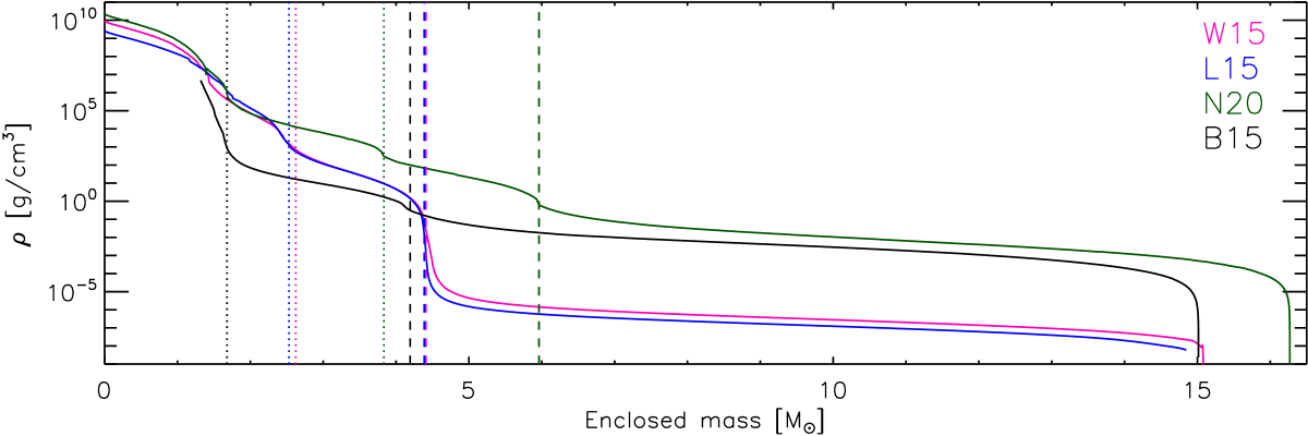
Figure 1: Density as a function of enclosed mass for all four considered progenitor stars at the onset of core collapse. The vertical dotted and dashed lines mark the locations of the C+O/He and He/H composition interfaces,respectively, for each progenitor star.

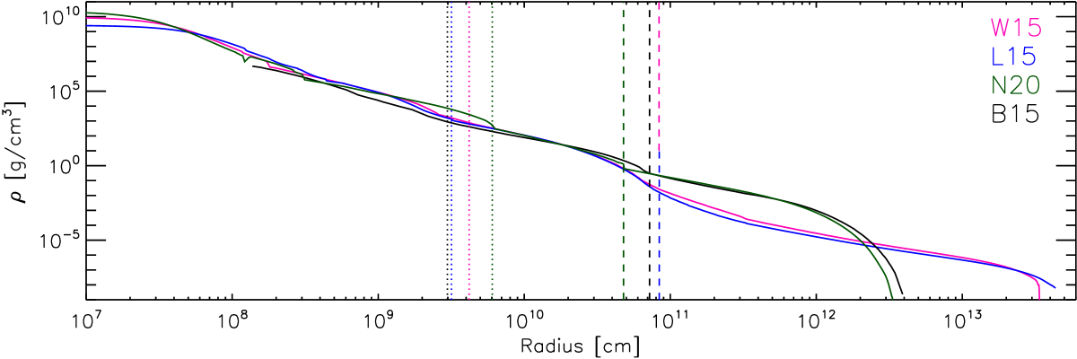
Figure 2: Same as Fig. 1, but as a function of radius.

In the present study, we consider only a subset of the explosion models of Wongwathanarat et al. (2013), namely models W15-1, W15-2, L15-1, L15-2, N20-4, B15-1, and B15-3 (see Tab. 1), where the first three characters of the model name indicate the respective progenitor star. W15 denotes the 15 $M_{\odot}$ RSG model s15s7b2 of Woosley & Weaver (1995), L15 a 15 $M_{\odot}$ RSG model evolved by Limongi et al. (2000), N20 a 20 $M_{\odot}$ BSG progenitor model for SN 1987A by Shigeyama & Nomoto (1990), and B15 a corresponding 15 $M_{\odot}$ BSG model by Woosley et al. (1988). We note that the mass of model N20 is reduced from a main-sequence value of $20\,M_{\odot}$ to $16.3\,M_{\odot}$ at the onset of core collapse due to mass loss.

Figs. 1 and 2 show the density as a function of enclosed mass and radius, respectively, for all four progenitors at the onset of core collapse. We define the locations of the C+O/He and He/H composition interfaces as those positions at the bottom of the He and H layers of the star where the He and H mass fractions drop below half of their maximum values in the respective layer. The radial coordinates of the C+O/He and He/H interfaces are denoted as $R_{\mathrm{C+O/He}}$ and $R_{\mathrm{He/H}}$, respectively.

The density profiles of the two RSG progenitors W15 and L15 are overall quite similar, but the density drops more steeply at the He/H composition interface in model L15 and the hydrogen envelope of this model is more dilute, i.e., its envelope is more extended than that of model W15. The density of the two BSG models B15 and N20 decreases much less steeply at the He/H interface than in the RSG models. Model N20 has the largest densities inside the C+O core which is also the most massive C+O core ($\approx 3.8\,M_{\odot}$) of all models, while model B15 possesses the least massive C+O core ($\approx 1.7\,M_{\odot}$).

In order to simulate the evolution of the SN explosion well beyond the epoch of shock revival we mapped the data of the seven 3D explosion models described above onto a larger computational grid at time $t_{\mathrm{map}}$ (see Table 1). Defining the (time-dependent) explosion energy of a model as the sum of the total (i.e., internal plus kinetic plus gravitational) energy of all grid cells where this energy is positive, the explosion energy at the time of mapping $E_{\mathrm{map}}$ ranges from 1.12 B to 1.74 B (where 1B$\equiv 10^{51}$ erg; see Table 1). The explosion time $t_{\mathrm{exp}}$, also provided in Table 1, is defined as the moment when the explosion energy exceeds a value of $10^{48}$ erg, which roughly coincides with the time when the average shock radius becomes larger than 400–500 km.

Because the hydrodynamic timescale varies strongly through the exploding star we also move the inner grid boundary (located close to a radius of 15 km in models W15, N20 and B15, and 25 km in model L15 at time $t_{\textrm{map}}$; see Table 1 in Wongwathanarat et al. (2013)) to a larger radius of $R_{\textrm{ib}}=500$ km at the time of mapping. This relaxes the CFL time step constraint imposed by the high sound speed in the vicinity of the proto-neutron star. Moreover, during the course of the simulations we moved the inner grid boundary repeatedly to larger radii, thereby further relaxing the CFL condition. This procedure (see Sect. 2.2) allowed us to complete the otherwise computationally too expensive simulations with a reasonable amount of computing time.

For comparison with the work of HJM10 we performed two additional 3D simulations where the numerical setup differed slightly from the standard one described above (see Sect. 3.1).

2.2 Numerics

We performed our simulations with Prometheus, an explicit, finite-volume Eulerian multi-fluid hydrodynamics code (Fryxell et al. 1991; Müller et al. 1991b, a). It solves the multi-dimensional Newtonian hydrodynamic equations using dimensional splitting (Strang 1968), piecewise parabolic reconstruction (PPM; Colella & Woodward 1984), a Riemann solver for real gases (Colella & Glaz 1985), and the consistent multi-fluid advection scheme (CMA; Plewa & Müller 1999). To prevent odd-even decoupling inside grid zones with strong grid-aligned shocks (Quirk 1994), we used the AUSM+ fluxes of Liou (1996) instead of the fluxes computed with the Riemann solver. We further utilized the “Yin-Yang” overlapping grid technique (Kageyama & Sato 2004; Wongwathanarat et al. 2010a) instead of a spherical polar (latitude-longitude) grid to cover the computational domain, because it alleviates the CFL condition resulting from the coordinate singularity of the polar grid at the poles. In this way we could use in our simulations time steps that were several ten times larger than for the case of a spherical polar computational grid with similar lateral resolution. The Yin-Yang grid also prevents numerical artifacts which might arise near the polar axis, where a boundary condition has to be imposed when a spherical polar grid is used.

Newtonian self-gravity was taken into account by solving the integral form of Poisson’s equation with a multipole expansion method as described in Müller & Steinmetz (1995). In addition, a point mass was placed at the coordinate origin to account for the (monopole part of the) gravity of the proto-neutron star and of the matter excised successively from our computational domain.

The computational grid covers the full $4\pi$ solid angle. Initially, it extends in radius from $R_{\mathrm{ib}}$=500 km to the stellar radius $R_{\ast}$ (see Table 1). The radial grid is logarithmically spaced and initially has a resolution of 5 km at the inner grid boundary. $R_{\mathrm{ib}}$ is fixed during the first 2 s of the simulations and thereafter successively shifted to larger radii, removing the respective innermost radial grid zone whenever $R_{\mathrm{ib}}$ becomes smaller than 2% of the minimum radius of the (aspherical) SN shock. This reduces the number of radial grid zones in the course of a simulation, thereby speeding it up. We cease the movement of the inner radial boundary at 10 000 s and 60 000 s for the BSG and RSG models, respectively. When the SN shock approaches the stellar surface we extend the computational domain to $R_{\mathrm{ob}}=10^{9}$ km in order to continue the simulation beyond shock breakout. The circumstellar conditions assumed at $r>R_{\ast}$ will be described in the next subsection.

In the simulations performed with the W15 and L15 progenitors we used 2590 radial zones for $500\,\mathrm{km}\leq r\leq 10^{9}$ km, while we used 3034 and 2957 zones in the cases of the N20 and B15 progenitors, respectively. This yields a relative radial resolution $\Delta r/r$ of better than 1% at all radii. The angular resolution is 2^∘ in all models. At the end of a simulation the number of radial grid zones is more than halved, while only $\sim 10^{-6}$ of the initial computational volume is cut off.

2.3 Input physics

We performed our longtime simulations with the tabulated equation of state (EoS) of Timmes & Swesty (2000) taking into account arbitrarily degenerate and relativistic electrons and positrons, photons, and a set of nuclei. The nuclei, consisting of protons, $\alpha$-nuclei, and a tracer nucleus $X$ which traces the production of a neutron-rich (non-alpha) nucleus in neutron-rich environments ($Y_{e}<0.49$), are treated as a mixture of ideal Boltzmann gases which are advected by the flow. Moreover, the mass fractions of the $\alpha$-nuclei and of the tracer nucleus may also change during the evolution due to nuclear reactions, which are described by an $\alpha$-chain reaction network (Kifonidis et al. 2003; Wongwathanarat et al. 2013).

Initially, there are no protons in the matter inside the shock (the proton mass fraction $X_{\mathrm{p}}$ is set to a floor value of $10^{-10}$). Outside of the shock the proton abundance is given by that of the respective progenitor model, and is only of relevance in the hydrogen envelope. The mass fractions of the $\alpha$-nuclei and the tracer $X$ are the ones of the corresponding explosion simulation at the time of mapping (see Sect. 2.1). We note here that in the explosion simulations we also integrated an $\alpha$-network with the flow. Its only purpose was, however, to provide abundance information, i.e., in these simulations the network was neither energetically nor through composition changes coupled to the hydrodynamics and the EoS .

Two versions of the network are available in our code: one involves the 13 $\alpha$-nuclei from ⁴He to ⁵⁶Ni plus the tracer nucleus $X$, and a second, smaller network which does not contain the $\alpha$-nuclei ³²S, ³⁶Ar, ⁴⁸Cr, and ⁵²Fe. The smaller network was used to simulate the W15 and L15 models. The network is solved in grid cells whose temperature is within the range of $10^{8}$ K – $8\times 10^{9}$ K. Once the temperature drops below $10^{8}\,$K, all nuclear reactions are switched off because they become too slow to change the nuclear composition on the explosion timescale. To prevent the nuclear burning timestep becoming too small, we also do not perform any network calculations in zones with temperatures above $8\times 10^{9}\,$K. We assume a pure $\alpha$-particle composition in these zones.

We neglect the feedback of the nuclear energy release in the network calculations on the hydrodynamic flow. This energy release is of minor relevance for the dynamics because the production of $\approx 0.1\,M_{\odot}$ of ⁵⁶Ni means a contribution of only $\leavevmode\nobreak\ 10^{50}\,$erg to the explosion energy. It is important to note that our model parameters are chosen to give energetic explosions already by neutrino energy input.

When the density (temperature) in a zone drops below $10^{-10}$ g cm^-3 ($10^{4}$ K), which is the smallest value given in the EoS table of Timmes & Swesty (2000), we switch to a simpler EoS taking into account only a set of ideal Boltzmann gases and blackbody radiation. The pressure $p$ and specific internal energy $e$ are then given by

$$p = \frac{1}{3}aT^{4}+\frac{k_{\mathrm{B}}}{\mu m_{\mathrm{H}}}\rho T\,,$$ (1)

$$e = \frac{aT^{4}}{\rho}+\frac{3}{2}\frac{k_{\mathrm{B}}}{\mu m_{\mathrm{H}}}T\,,$$ (2)

where $a,\rho,T,k_{\mathrm{B}},\mu$, and $m_{\mathrm{H}}$ are the radiation constant, the density, the temperature, Boltzmann’s constant, the mean molecular weight , and the atomic mass unit, respectively.

After mapping we continued to take into account the effect of neutrino heating near the proto-neutron star surface by means of a boundary condition that describes a spherically symmetric neutrino-driven wind injected through the inner grid boundary. Since the wind is spherically symmetric it does not affect the development of asymmetries in the ejecta. The hydrodynamic and thermodynamic properties of the wind are derived from the angle-averaged state variables of the explosion models of Wongwathanarat et al. (2013) at $r=500\,$km.

In most of our simulated models we imposed (for simplicity) a constant wind boundary condition, where all wind quantities are time independent. We also simulated two models with time-dependent wind quantities (see Tab. 2). In these latter models we assumed a constant wind velocity $v_{\mathrm{w}}$. This leads to a power-law wind boundary condition where the time-dependent density $\rho_{\mathrm{w}}$, specific internal energy $e_{\mathrm{w}}$, and pressure $p_{\mathrm{w}}$ are given by

$$\rho_{\mathrm{w}}(t) = \rho_{\mathrm{w}}(t_{\mathrm{map}})\left(\frac{t}{t_{\mathrm{map}}}\right)^{-7/2}\,,$$ (3)

$$e_{\mathrm{w}}(t) = e_{\mathrm{w}}(t_{\mathrm{map}})\left(\frac{t}{t_{\mathrm{map}}}\right)^{-7/6}\,,$$ (4)

and

$$p_{\mathrm{w}}(t) = \frac{1}{3}e_{\mathrm{w}}(t)\,\rho_{\mathrm{w}}(t)\,,$$ (5)

with $t_{\mathrm{map}}$ from Tab. 1. The choice of the power-law indices in Eqs. (3) and (4) is motivated by an extrapolation of the density and internal energy evolution at $r=500\,$km. We refer to the two kinds of wind models in the following by adding a suffix “cw” for the constant wind and “pw” for the power-law wind to the model names, respectively (see Tab. 2).

We applied both wind boundary conditions for a time period of 2 s and then switched to a reflecting boundary condition. At the outer radial grid boundary we used a free outflow condition at all times. We tested the influence of the wind boundary conditions with two simulations (B15-1-cw and B15-1-pw; see Sect. 5.1 for details), which represent quite an extreme case for the difference between both. The test showed that the morphology of the metal-rich ejecta does not depend on the choice of the wind boundary condition, although in the power-law wind model the explosion energy saturates earlier at a considerably lower value, and the maximum Ni velocities are almost a factor of two smaller than in the constant wind model (see Tab. 2, and discussion in Sect. 5.2 and 5.3.4).

To follow the evolution beyond shock breakout we embedded our stellar models in a spherically symmetric circumstellar environment resembling that of a stellar wind. In this environment, the density and temperature distribution of the matter, which is assumed to be at rest, is given for any grid cell $i$ with $r_{i}>R_{\ast}$ by

$$\rho_{\mathrm{e}}(r) = \rho_{0}\left(\frac{R_{\ast}}{r}\right)^{2}\,,$$ (6)

$$T_{\mathrm{e}}(r) = T_{0}\left(\frac{R_{\ast}}{r}\right)^{2}$$ (7)

with $\rho_{0}=3\times 10^{-10}$ g cm^-3 and $T_{0}=10^{4}$ K. The stellar radius $R_{\ast}$ is given in Tab. 1.

3 Comparison with HJM10

Before discussing the set of ”standard” 3D simulations (see Sect. 5.1), we first consider two additional 3D simulations that we performed specifically to compare the results with those of the 3D simulation of HJM10. The numerical setup and the input physics differ slightly from the standard one used in all our other simulations presented here, so that they closely resemble those described in HJM10, except for the utilization of the Yin-Yang grid in our simulations.

3.1 Simulation setup

The simulations are initialized from the 3D explosion model of Scheck (2007) that results from the core collapse of the BSG progenitor model B15. Scheck (2007) simulated the evolution in 3D from 15 ms until 0.595 s after core bounce using a spherical polar grid with 2^∘ angular resolution and 400 radial grid zones. To alleviate the CFL time step constraint he excised a cone of 5^∘ half-opening angle around the polar axis from the computational domain. The explosion energy was $0.6\,$B at the end of the simulation, but had not yet saturated. Scheck (2007) neglected nuclear burning and used the EoS of Janka & Müller (1996) with four nuclear species ($n$, $p$, ⁴He, and ⁵⁴Mn), assumed to be in nuclear statistical equilibrium.

We mapped the explosion model of Scheck (2007) onto the Yin-Yang grid using two grid configurations with $1200(r)\times 92(\theta)\times 272(\phi)\times 2$ and $1200(r)\times 47(\theta)\times 137(\phi)\times 2$ zones. This corresponds to an angular resolution of 1^∘ (model H15-1deg) and 2^∘ (model H15-2deg), respectively. Since a cone around the polar axis was excised in the explosion model of Scheck (2007), we supplemented the missing initial data using tri-cubic spline interpolation. The radial grid extends from 200 km to near the stellar surface, the fixed outer boundary of the Eulerian grid being placed at $3.9\times 10^{7}\,$km. We imposed a reflective boundary condition at the inner edge of the radial grid, and a free-outflow boundary condition at the outer one. During the simulations we repeatedly moved the inner boundary outwards, as described in Sect. 2.2.

As in HJM10 we artificially boosted the explosion energy to a value of 1 B by enhancing the thermal energy of the post-shock matter in the mapped ”initial” state (at 0.595 s). We did neither take self-gravity nor nuclear burning into account. We advected eight nuclear species ($n$, $p$, ⁴He, ¹²C, ¹⁶O, ²⁰Ne, ²⁴Mg, and ⁵⁶Ni) redefining the ⁵⁴Mn in the explosion model of Scheck (2007) as ⁵⁶Ni in our simulations.

The setups employed for our two H15 simulations and the simulation of HJM10 differ only with respect to the grid configuration. HJM10 used a spherical polar grid excising a cone of 5^∘ half-opening angle around the polar axis as Scheck (2007), while we performed our present simulations with the Yin-Yang grid covering the full 4$\pi$ solid angle. Our model H15-1deg has the same angular resolution as the 3D simulation of HJM10. We note that in the simulation of HJM10 the reflecting boundary condition imposed at the surface of the excised cone might have affected the flow near this surface, while our simulations based on the Yin-Yang grid avoid such a numerical problem.

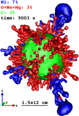
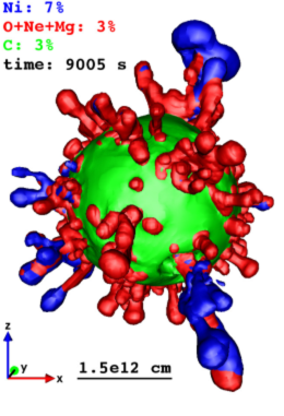
Figure 3: Isosurfaces of constant mass fractions at t$\approx$9000 s for models H15-1deg (left) and H15-2deg (right), respectively. The mass fractions are 7% for ⁵⁶Ni (blue), and 3% for ¹⁶O+²⁰Ne+²⁴Mg (red) and ¹²C (green). The morphology is almost identical to that shown in the lower left panel of Fig. 2 in HJM10, except for some additional small-scale structures in the better resolved model. There are two pronounced nickel plumes (blue) visible on the right, which travel at velocities up to 3800 km s^-1 and 4200 km s^-1 in model H15-2deg and H15-1deg, respectively, and two smaller nickel fingers on the left.

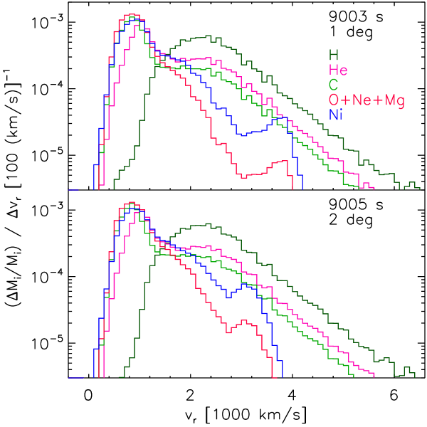
Figure 4: Normalized mass distributions of ¹H (dark green), ⁴He (magenta), ¹²C (green), ¹⁶O+²⁰Ne+²⁴Mg (red), and ⁵⁶Ni (blue) versus radial velocity $v_{r}$ for models H15-1deg (top) and H15-2deg (bottom). For all elements the distributions (especially of model H15-1deg) agree very well with those shown in the bottom right panel of Fig. 6 in HJM10.

3.2 Results

Fig. 3 shows isosurfaces of constant mass fractions of ⁵⁶Ni, ”oxygen”, and ¹²C about 9000 s after core bounce for model H15-1deg (left) and H15-2deg (right), respectively. Note that as in HJM10, we denote in this section by ”oxygen” the sum of the mass fractions of ¹⁶O , ²⁰Ne, and ²⁴Mg. At first glance, both simulations exhibit similar RT structures. Two pronounced nickel (blue) plumes, a few smaller nickel fingers, and numerous ”oxygen” (red) fingers burst out from a quasi-spherical shell of carbon (green). The maximum radial velocity of the pronounced nickel plumes is about 4200 km s^-1 in model H15-1deg and about 3800 km s^-1 in model H15-2deg (Fig. 4). However, while at the tips of these nickel plumes well-defined mushroom caps grow in model H15-1deg, they are less developed in model H15-2deg, because the responsible secondary Kelvin-Helmholtz (KH) instabilities are not captured very well in the run with the lower angular resolution.

There are also more ”oxygen” fingers in model H15-1deg than in model H15-2deg. Nevertheless, these fingers grow along exactly the same directions in both simulations. Comparing the spatial distribution of RT fingers in Fig. 3 and the lower left panel of Fig. 2 in HJM10 one also recognizes striking similarities. Besides the two pronounced nickel plumes, which grow into the same directions, there are also two smaller nickel fingers pointing to the left side, which are present in the 3D simulation of HJM10, too. Even the distribution of the small ”oxygen” fingers in HJM10’s 3D simulation is captured well by both of our H15 models.

Fig. 4 displays the normalized mass distributions of ¹H, ⁴He, ¹²C, ”oxygen”, and ⁵⁶Ni versus radial velocity for model H15-1deg (top) and H15-2deg (bottom). Although the distributions from both simulations agree well for all nuclear species, one can notice some differences at the high-velocity tail of the nickel distribution and at the low-velocity tail of the hydrogen distribution. The fastest nickel moves with a velocity of about 4200 km s^-1 in model H15-1deg, while it is about 10% slower in model H15-2deg. For the former model hydrogen is mixed down to radial velocities of $\leavevmode\nobreak\ 500\,$km s^-1, while the minimum velocity amounts to $\leavevmode\nobreak\ 700\,$km s^-1 in model H15-2deg.

These results are in excellent agreement with those of HJM10 (see the bottom right panel of their Fig. 6), except for some minor differences. The peak radial velocity of nickel is about 4500 km s^-1 in the model of HJM10, i.e., roughly 10% higher than in model H15-1deg. The slowest hydrogen moves with about 300 km s^-1 in their model, i.e., it is slightly slower than in ours.

We attribute these differences to the numerical resolution, which is higher in the 3D model of HJM10 in the polar regions, and whose influence can be seen by comparing our models H15-1deg and H15-2deg. By construction the linear size of the angular zones is almost uniform for the Yin-Yang grid, while it decreases considerably near the poles for the spherical polar grid. Thus, although using the same angular grid spacing of $1^{\circ}$ in both studies, the spatial resolution is lower in our H15-1deg simulation in the polar regions than in the simulation of HJM10. Consequently, the regions where the two pronounced nickel plumes are located are better resolved in their simulation than in ours.

The comparison of our results with those of HJM10 allows for two conclusions:

• The overall similarity (qualitatively and quantitatively) of the results of models H15-1deg and H15-2deg suggests that an angular resolution of 2^∘ is already sufficient for our current study, which aims at capturing neither details of small-scale structures nor determining the precise peak velocities of small fractions of heavy elements in the ejecta. Using an angular resolution of 2^∘ allows us to perform a parameter study changing both the explosion energy and the progenitor with a reasonable amount of computing time.

• The similarity of the ejecta asymmetries and radial mixing confirms that the long-time evolution of the SN is determined by the initial asymmetries imprinted by the explosion mechanism rather than by stochastic effects of the secondary RT instabilities growing at the composition interfaces. Characteristic features of the earliest phases of the explosion therefore map into the ejecta morphology at later times.

• The peak velocities of heavy elements and the minimal velocities of inward mixed hydrogen are more extreme for better resolved models. Numerical viscosity in less well resolved models reduces the extent of radial mixing.

In Sect. 5 we will investigate how this mapping depends on the progenitor star and the progenitor-specific interaction of initial explosion asymmetries with the RT instabilities that develop at the composition interfaces after the passage of the outgoing SN shock wave.

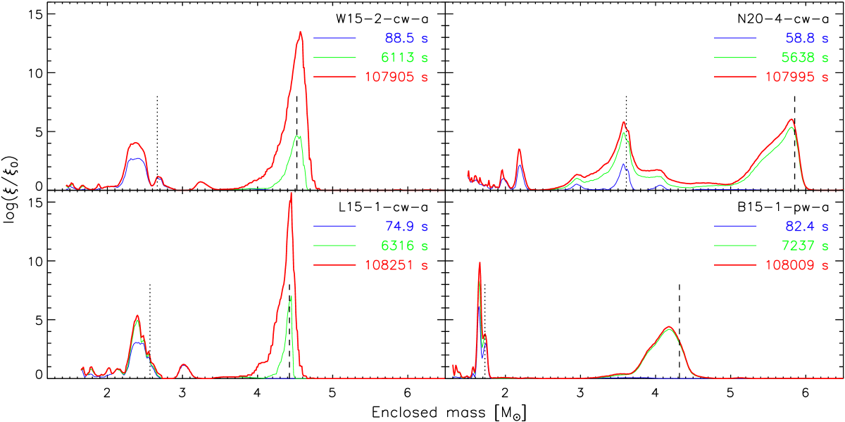
Figure 5: Time-integrated RT growth factors versus enclosed mass for the 1D models W15-2-cw-a, L15-1-cw-a, N20-4-cw-a, and B15-1-pw-a at the given times. The vertical dotted and dashed lines mark the mass coordinates of the C+O/He and He/H interfaces (defined in Sect. 2.1), respectively.

4 One-dimensional models: Linear stability analysis

While propagating through the star the velocity of the SN shock varies, because it accelerates or decelerates more or less strongly depending on the density stratification it encounters, which in turn depends on the progenitor star. In particular, whenever the density gradient is steeper than $r^{-3}$ (i.e. $d(\rho r^{3})/dr<0$), a shock wave accelerates according to the blast-wave solution (Sedov 1959). This condition is fulfilled near composition interfaces where the density varies most strongly, especially near the C+O/He and He/H composition interfaces. An acceleration at the interface follows a deceleration in the overlying stellar layers, which causes a density inversion in the post-shock flow, i.e., a dense shell forms. Such shells are prone to RT instabilities, because they are associated with density and pressure gradients of opposite signs (Chevalier 1976).

To aid us with the analysis of the 3D simulations, we have computed the linear RT growth rates for each of our progenitor stars. For an incompressible fluid it is given by (Bandiera 1984; Benz & Thielemann 1990; Müller et al. 1991b)

$$\sigma_{\mathrm{RT}}=\sqrt{-\frac{\partial p}{\partial r}\frac{\partial\rho}{\partial r}}.$$ (8)

We monitor the growth of RT instabilities by calculating the time-integrated growth factor

$$\frac{\xi}{\xi_{0}}(t)=\exp{\left(\int_{0}^{t}\,\sigma_{\mathrm{RT}}\,dt^{\prime}\right)}$$ (9)

at fixed Lagrangian mass coordinates, which tells by how much an initial perturbation with an amplitude $\xi_{0}$ would grow until time $t$.

Tracking a fixed mass coordinate is not easily feasible in our 3D Eulerian simulations, especially when the flow shows strong asymmetries. Thus, we performed four 1D simulations, one for each of the considered progenitor stars, based on the angle-averaged profiles of the 3D models W15-2, L15-1, N20-4, and B15-1 at time $t_{\mathrm{map}}$, which were also used for our 3D runs to late times (see Sect. 5.1). The numerical setup for these 1D simulations was identical to that used in the 3D simulations described in Sect. 2. The constant wind boundary condition (see Sect. 2.3) was imposed in the simulations using the explosion models W15-2, L15-1, and N20-4, while the power-law wind boundary condition was applied in the run with the explosion model B15-1. We denote the corresponding 1D simulations by W15-2-cw-a, L15-1-cw-a, N20-4-cw-a, and B15-1-pw-a, which gave rise to explosions with energies of $1.20\,$B, $1.53\,$B, $1.47\,$B, and $1.28\,$B, respectively .

Figure 5 displays the time-integrated RT growth factors as functions of enclosed mass for our 1D runs at three different times. The blue lines show the growth factors at the time when the SN shock crosses the C+O/He interface, which occurs between 60 s and 90 s depending on the model. The green lines give the growth factors at the time of shock breakout for the BSG models N20-4-cw-a and B15-1-pw-a, and at about 6000 s (i.e., roughly at the time of shock breakout in the BSG models; see Table 2) for the RSG models W15-2-cw-a and L15-1-cw-a. In these latter models the SN shock reaches the stellar surface only after about 90 000 s (see Table 2). The red lines, finally, display the growth factors at the end of the simulations ($\approx 10^{5}\,$s).

The growth factors show a characteristic behavior near the C+O/He and He/H interfaces, which depends on the density profile of the respective progenitor.

In the RSG models W15 and L15 the growth factor is very large at the He/H interface ($\log(\xi/\xi_{0})\approx 14\ldots 16$). It is largest in model L15, since the density gradient at the He/H interface is steepest in this model. In both progenitors the growth rate is much smaller at the C+O/He interface ($\log(\xi/\xi_{0})\approx 4\ldots 5$), because the density gradient is shallower there than at the He/H interface.

In the BSG models N20 and B15 the RT growth factor at the He/H interface is much smaller ($\log(\xi/\xi_{0})\approx 5\ldots 6$) than for the RSG progenitors, because the density decreases very little in these progenitors at the He/H interface. Only for the B15 progenitor the RT growth rate is higher at the C+O/He interface than at the He/H interface, reaching already a value of $\log(\xi/\xi_{0})\approx 6$ by the time when the SN shock reaches the edge of the C+O core.

In all models, the RT growth factors continue to grow at the C+O/He interface while the SN shock is propagating through the hydrogen envelope, but they do not significantly increase in both BSG models at the He/H interface after the SN shock has broken out of the stellar surface. The latter result holds despite of a much longer integration time, implying saturation of the growth of RT instabilities at relatively much earlier times than in the RSG models.

We point out that the results presented in Fig. 5 can only provide a qualitative criterion for the relative strength of the expected RT growth in different layers of the progenitor star. The values of the linear growth factors depend on the flow structure in the post-shock layers which, in turn, depends on the explosion energy. The fact that the models shown in Fig. 5 explode with comparable energies makes the comparison of the RT growth factors among these models meaningful. More importantly, we have calculated the RT growth rates by means of linear perturbation theory of 1D models, while in multi-D simulations the instabilities will quickly enter the non-linear regime. Nevertheless, we find that this linear stability analysis is particularly useful in understanding the results of our 3D runs, which we will discuss in the next section.

Table 2: Some properties of the simulated 3D models at the given times (see text for details).

progenitor	3D	$t_{\mathrm{surf}}$	$E_{\mathrm{exp}}$	avg${}^{\mathrm{(max)}}_{\mathrm{(min)}}$ $R_{\mathrm{s}}$	$M_{\mathrm{Ni}}$ $(M_{\mathrm{Ni}+X})$	$v_{\textrm{max}}(\textrm{Ni})$	$\langle v\rangle_{1\%}(\textrm{Ni})$
type	model	[s]	[B]	[$10^{6}\,$km]	[$M_{\odot}$]	[$10^{3}\,$km s-1]	[$10^{3}\,$km s-1]
RSG	W15-1-cw	84974	1.48	$389^{(443)}_{(355)}$	0.05 (0.13)	5.29	3.72
	W15-2-cw	85408	1.47	$393^{(458)}_{(349)}$	0.05 (0.14)	4.20	3.47
	L15-1-cw	95659	1.75	$478^{(530)}_{(448)}$	0.03 (0.15)	4.78	3.90
	L15-2-cw	76915	2.75	$475^{(500)}_{(458)}$	0.04 (0.21)	5.01	4.51
BSG	N20-4-cw	5589	1.65	$39.7^{(43.6)}_{(35.6)}$	0.04 (0.12)	2.23	1.95
	B15-1-cw	5372	2.56	$41.5^{(43.6)}_{(39.5)}$	0.05 (0.11)	6.25	5.01
	B15-1-pw	7258	1.39	$42.7^{(45.7)}_{(40.0)}$	0.03 (0.09)	3.34	3.17
	B15-3-pw	8202	1.14	$48.1^{(51.1)}_{(44.7)}$	0.03 (0.08)	3.18	2.95

5 Three-dimensional models

5.1 Model overview

We have simulated eight 3D models (see Table 2) using our four progenitor stars, two of which are RSG and two of which are BSG (see Sect. 2.1). The first part of the model name refers to the model for the initial neutrino-driven onset of the explosion (e.g., W15-1), while the second part denotes the kind of neutrino-driven wind boundary condition imposed in the respective long-time simulation (i.e., either cw or pw).

The RSG models W15-1-cw and W15-2-cw are initialized from two explosion models, which differ only in the initial perturbation pattern that was imposed to break the spherical symmetry of the 1D collapse model at 15 ms after core bounce (for details, see Wongwathanarat et al. (2013)). Although both models have nearly identical explosion energies, the ejecta asymmetries developed differently in these models during the shock revival phase because of the chaotic nature of the non-radial hydrodynamic instabilities. Hence, comparing models W15-1-cw and W15-2-cw, we can infer how asymmetries developing during the revival of the SN shock influence the ejecta distribution at late times when all other conditions are the same.

The RSG models L15-1-cw and L15-2-cw represent two cases of significantly different explosion energies of the L15 progenitor, the explosion of model L15-2-cw being approximately 60% more energetic and also developing faster than the one of model L15-1-cw. Moreover, the shock surface is less deformed, appearing almost spherical, in explosion model L15-2 than in L15-1, because low-mode instabilities have less time to grow during the shock revival phase in the former explosion model.

The BSG model N20-4-cw is the only model in our set which does not have a 15 but a 20 solar mass progenitor. Comparing its evolution with those of our other models we gain some insight into the influence of variations of BSG models for SN 1987A progenitors on the ejecta morphology.

To test the influence of the neutrino-driven wind boundary condition we simulated the BSG models B15-1-cw and B15-1-pw, which are both based on the explosion model B15-1. We chose this explosion model for the test, because the neutrino luminosities radiated by the neutron star at the time of mapping (1.1 s after bounce; see Table 1) are high in this model. This results in a denser and faster neutrino-driven wind at 500 km, where we placed the (initial) inner grid boundary in the long-time runs. The mapping time (1.1 s) was chosen to be earlier than in all other models, because the explosion timescales of the B15 models ($\approx 170$ ms) are smaller than in all other models (see Table 1). Finally, with model B15-3-pw we also simulated a lower-energy explosion of the B15 progenitor.

In Table 2 we summarize some properties of our 3D simulations at the shock breakout time $t_{\mathrm{surf}}$ (column 3), defined as the time when the minimum shock radius becomes larger than the initial stellar radius $R_{\ast}$. This time, which depends on the progenitor and the explosion energy (and to a lesser degree on the shock deformation), is less than two hours for the compact BSG progenitors, while it reaches and even exceeds 20 hours for the RSG progenitors. The additional quantities listed in the table are (columns 4 to 8):

• $E_{\mathrm{exp}}$ is the explosion energy defined as the sum of the total (internal plus kinetic plus gravitational) energy over all grid zones where the total energy is positive,

• $R_{\mathrm{s}}$ is the angle-averaged, maximum, and minimum value of the SN shock radius, respectively,

• $M$(Ni) is the total nickel mass, the number in the brackets giving an upper limit of the total mass of ⁵⁶Ni plus tracer $X$,

• $v_{\textrm{max}}$(Ni) is the maximum radial velocity on the outermost surface where the mass fraction of ⁵⁶Ni plus the tracer $X$ equals 3%, and

• $\langle v\rangle_{1\%}$(Ni) is the mass-weighted average radial velocity of the fastest 1% (by mass) of nickel.

The average SN shock radius, $\langle R_{\mathrm{s}}\rangle$, is given by

$$\langle R_{\mathrm{s}}\rangle=\frac{1}{4\pi}\int R_{\mathrm{s}}(\theta,\phi)\,d\Omega$$ (10)

with $d\Omega=\sin{\theta}\,d\theta\,d\phi$.

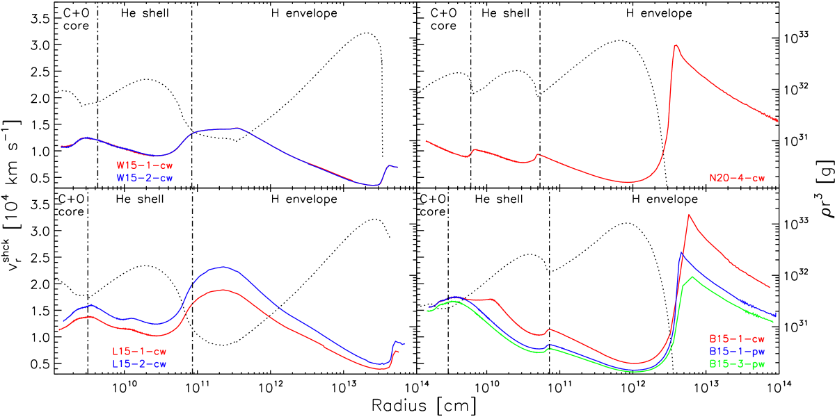
Figure 6: Radial velocity of the angle-averaged shock radius, $v_{r}^{\textrm{shck}}$, as a function of radius for our eight 3D models grouped in panels according to the respective progenitor model: W15 (top left), L15 (bottom left), N20 (top right), and B15 (bottom right). In each panel, we also display the corresponding distribution of $\rho r^{3}$ inside the progenitor star (black dotted line), the scale being given at the right hand side of the plot. The radii of the C+O/He and He/H composition interfaces in the progenitor star (defined in Sect. 2.1) are indicated by the vertical dash-dotted lines.

5.2 Dynamics of the supernova shock

Fig. 6 displays the radial velocity of the angle-averaged SN shock, $v_{r}^{\textrm{shck}}$, as a function of radius for our eight 3D models. To obtain this velocity we compute a backward finite difference in time of the angle-averaged shock radius $\langle R_{\mathrm{s}}\rangle$ using two subsequent outputs (typically 50 time steps apart). The figure also shows the $\rho r^{3}$ profile of each progenitor star (dotted lines), and the radial locations of the C+O/He and He/H composition interfaces (vertical dash-dotted lines).

Models W15-1-cw and W15-2-cw (Fig. 6, top left panel) have almost the same explosion energy and differ only in the initial seed perturbations. Hence, the propagation of the SN shock is similar in both models. It experiences two episodes of acceleration inside the star, one just before it crosses the C+O/He interface and another one at the He/H interface, followed by a strong deceleration in both cases. A third period of acceleration takes place right at the stellar surface.

The density structure of progenitor model L15 is overall quite similar to that of model W15, but the density decreases more rapidly with radius at the He/H interface in the former model. Therefore, the SN shock is accelerated more strongly at the He/H interface in model L15 than in model W15. According to Fig. 6 the shock speed increases nearly by a factor of two in model L15 and by about 50% in model W15. A comparison of models L15-1-cw and L15-2-cw (Fig. 6, lower right panel) shows that an increase of the explosion energy leads to the expected overall increase of the shock velocity, because the latter roughly scales as $\sqrt{E_{\mathrm{exp}}}$ (from which one expects about 25% higher values in model L15-2-cw).

Otherwise, the duration and the amount of acceleration/deceleration are very similar in both models.

The results obtained for the BSG progenitors N20 and B15 are displayed in the right panels of Fig. 6. In these models the SN shock experiences only a modest amount of acceleration at the He/H interface compared to models W15 and L15, because the density drops at that interface much less steeply in the BSG models than in the RSG models (see Fig.  2). The SN shock decelerates strongly while propagating through the helium shell of the B15 models, whereas it experiences only a modest deceleration in model N20-4-cw.

Comparing the dynamics of the SN shock in models B15-1-cw and B15-1-pw the effect of the neutrino-driven wind imposed at the inner radial grid boundary becomes obvious, in contrast to all other models with constant but much weaker wind power. Initially, the shock velocity is identical in both models. However, the constant supply of energy by the constant wind condition delays the saturation of the explosion energy in model B15-1-cw, i.e., the SN shock enters the blast-wave phase in model B15-1-cw later than in model B15-1-pw. The shock velocity remains almost constant in model B15-1-cw for $4\times 10^{9}\la r\la 11\times 10^{9}$ cm, although $\rho r^{3}$ increases in these layers. After the inflow of neutrino-driven wind has ceased and the explosion energy has saturated, the shock velocity behaves as in all other models and decreases (increases) with increasing (decreasing) $\rho r^{3}$ according to the blast-wave solution (Sedov 1959).

When the SN shocks reach the surfaces of the progenitor stars they encounter the steep density gradients prevailing there. They accelerate briefly, the acceleration being stronger in the BSG models than in the RSG models since the density gradients are steeper in the former models. Subsequently, the shocks decelerate again, because we assume a $r^{-2}$ density profile outside of the progenitor stars.

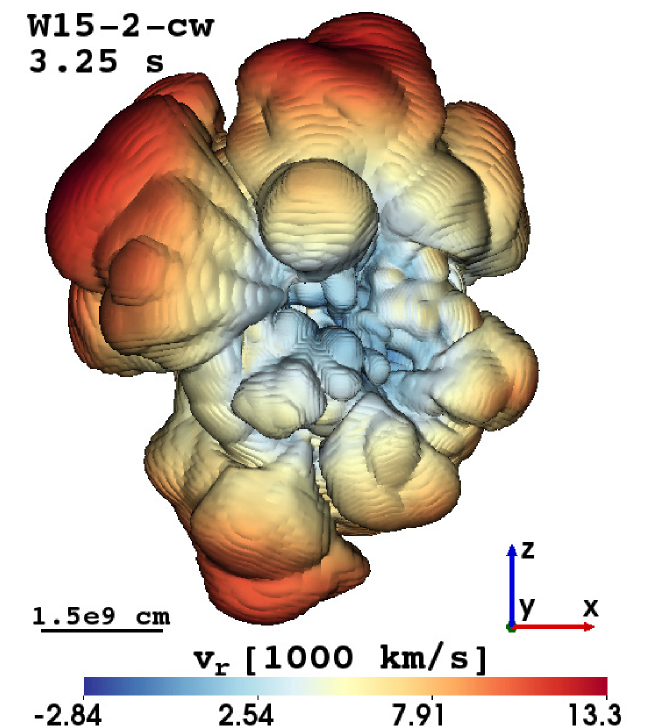
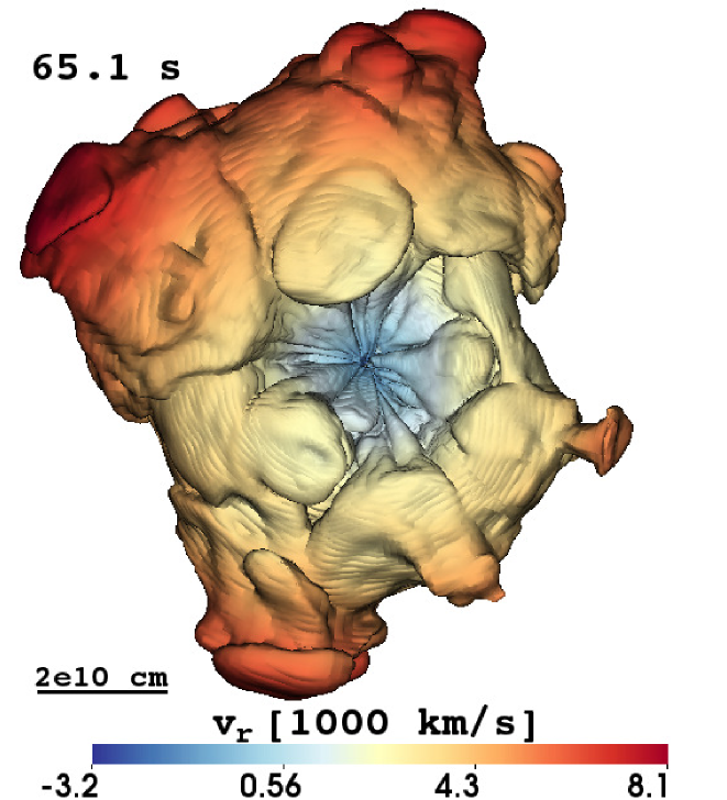
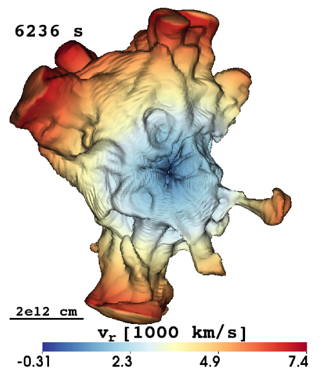
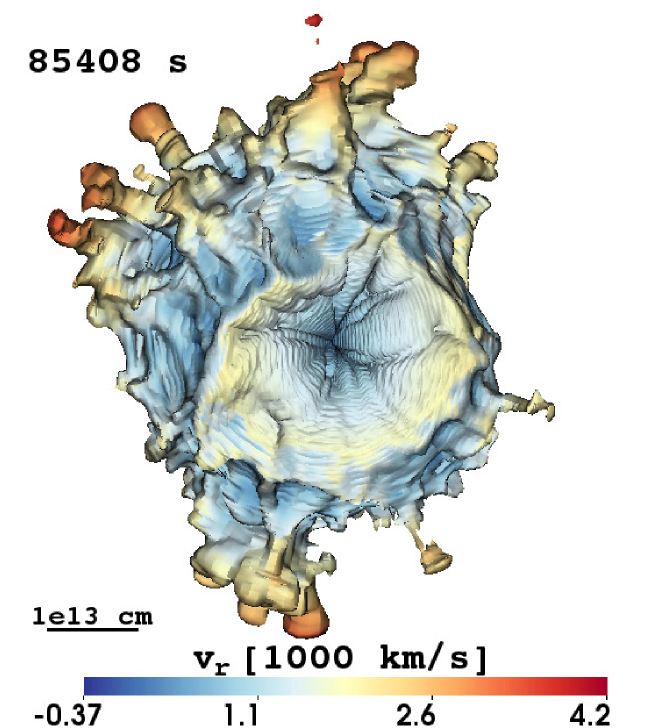
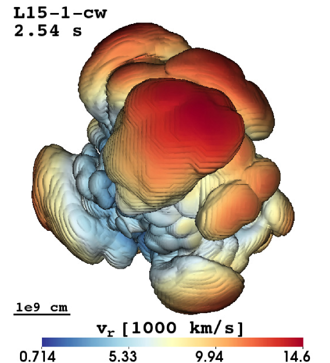
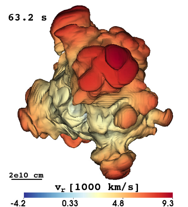
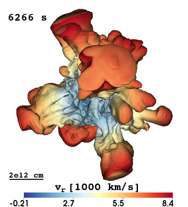
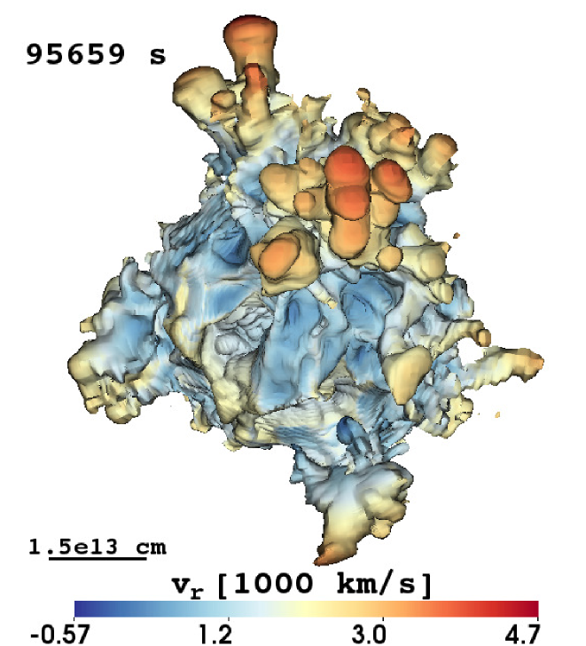
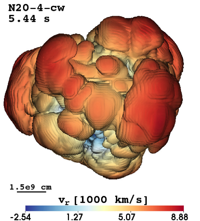
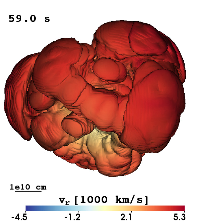
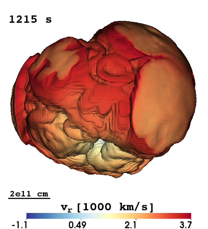
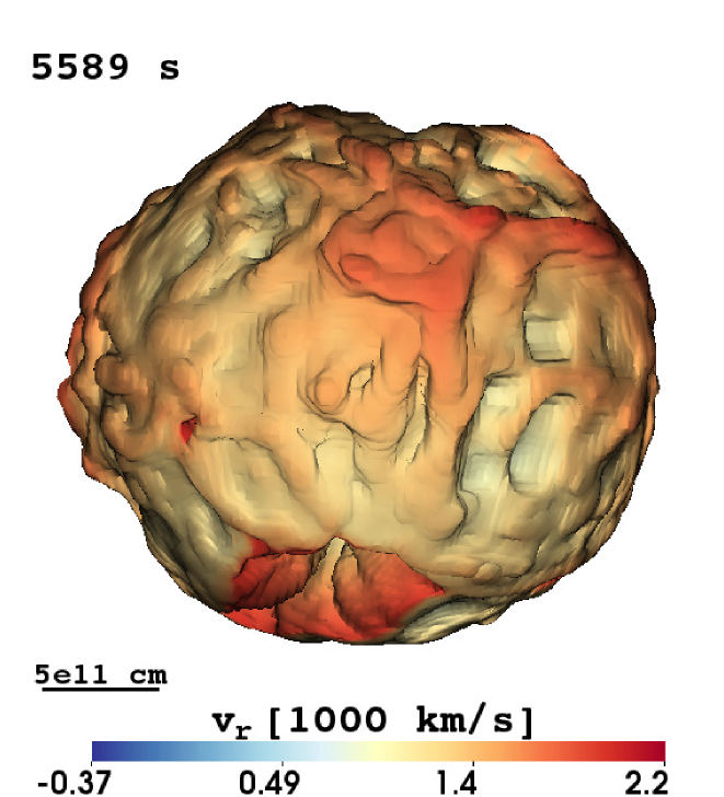
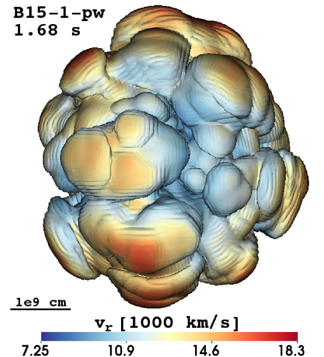
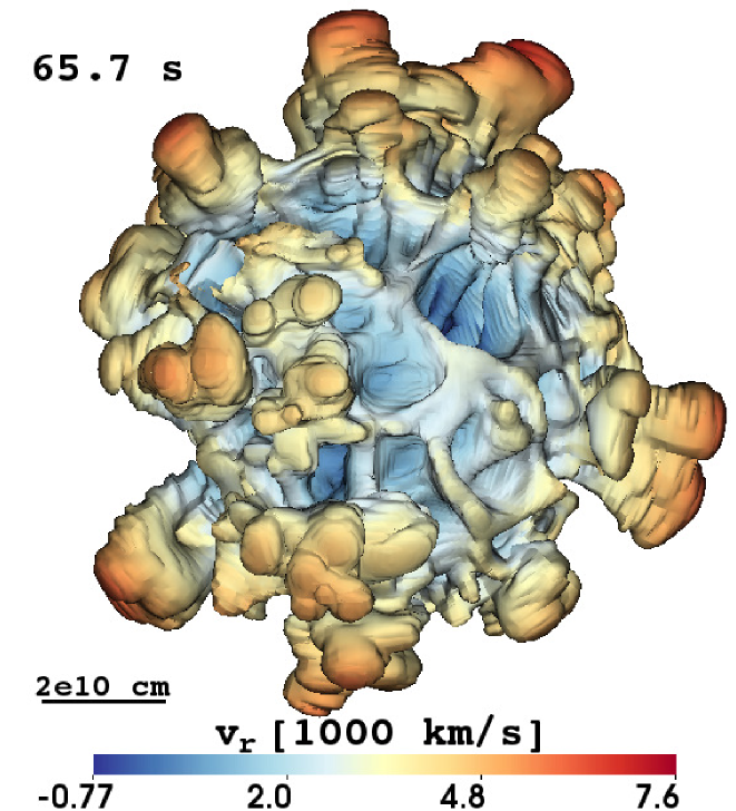
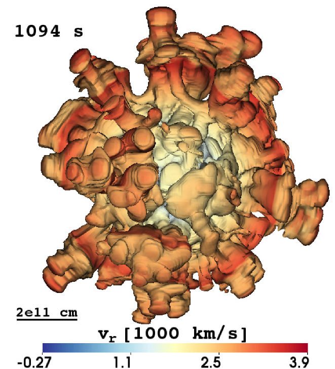
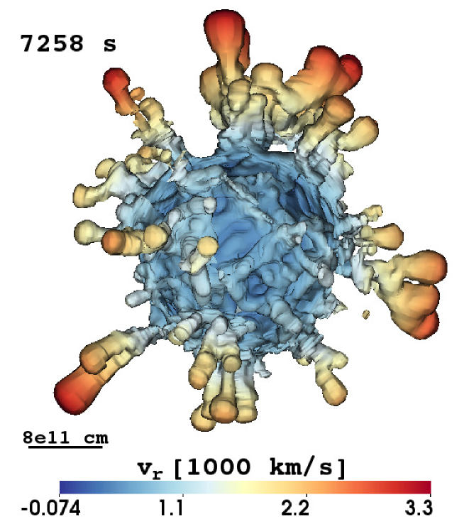
Figure 7: Snapshots displaying isosurfaces where the mass fraction of ⁵⁶Ni plus n-rich tracer $X$ equals 3% for model W15-2-cw (top row), L15-1-cw (second row), N20-4-cw (third row), and B15-1-pw (bottom row). The isosurfaces, which roughly coincide with the outermost edge of the neutrino-heated ejecta, are shown at four different epochs starting from shortly before the SN shock crosses the C+O/He composition interface in the progenitor star until the shock breakout time. The colors give the radial velocity (in units of km s^-1) on the isosurface, the color coding being defined at the bottom of each panel. In the top left corner of each panel we give the post-bounce time of the snapshot and in the bottom left corner a yardstick indicating the length scale. The negative y-axis is pointing towards the reader. One notices distinct differences in the final morphology of the nickel-rich ejecta of all models, which arise from their specific progenitor structures.

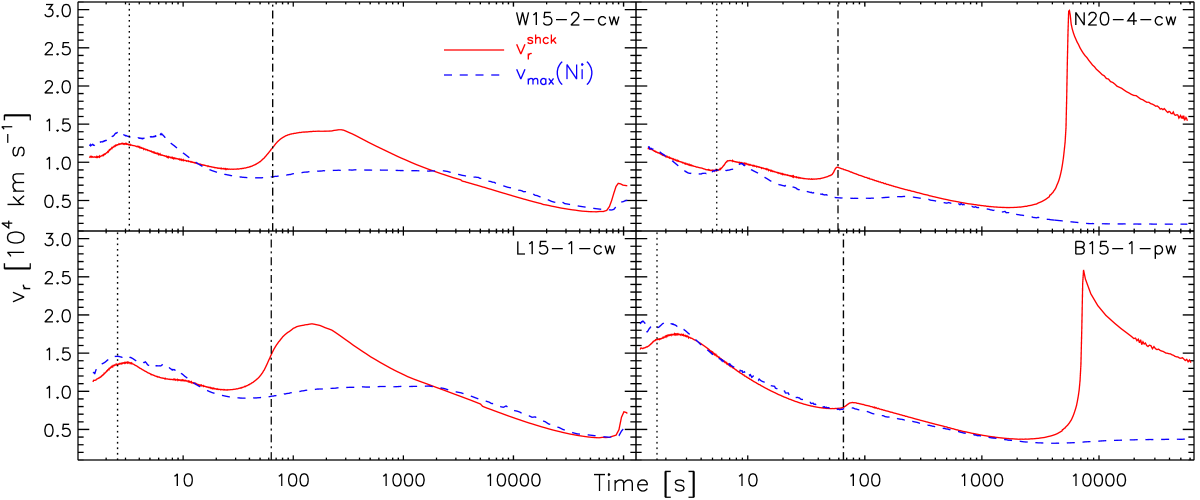
Figure 8: Time evolution of the radial velocity of the SN shock, $v_{r}^{\textrm{shck}}$ (solid red), and of the maximum radial velocity, $v_{\textrm{max}}(\textrm{Ni})$ (dashed blue), on the surface where the mass fraction of ⁵⁶Ni plus the n-rich tracer X equals 3%, for models W15-2-cw, N20-4-cw, L15-1-cw, and B15-1-pw, respectively. The vertical dotted and dashed-dotted lines mark the times when the shock crosses the C+O/He and He/H interfaces, respectively. These times are identical to those of the snapshots shown in the first and second column of Fig. 7.

5.3 Propagation of the neutrino-heated ejecta

We find interesting differences between the results obtained for different progenitor stars concerning the development of the early-time asymmetries which we trace by comparing the propagation history of the neutrino-heated ejecta bubbles. We illustrate these differences in Fig. 7 by means of snapshots displaying isosurfaces where the mass fraction of ⁵⁶Ni plus the n-rich tracer $X$ equals 3% for models W15-2-cw, L15-1-cw, N20-4-cw, and B15-1-pw (from top to bottom), respectively. We stress that Kifonidis et al. (2003) showed that ⁵⁶Ni is explosively produced in ”pockets” between the high-entropy bubbles of neutrino-heated matter, i.e., ⁵⁶Ni reflects the asymmetries of the first second of the explosion. All of these models yield comparable explosion energies with $1.39\,\mathrm{B}\leq E_{\mathrm{exp}}\leq 1.75\,$B. The isosurfaces, which roughly coincide with the outermost edge of the neutrino-heated ejecta, are shown at four epochs for each model.

Snapshots in column 1 and 2 of Fig. 7 display the isosurfaces at the moments when the SN shock is about to cross the C+O/He and He/H interfaces, i.e., when the maximum $R_{\mathrm{s}}$ becomes greater than $R_{\mathrm{C+O/He}}$ and $R_{\mathrm{He/H}}$, respectively. Column 3 depicts the isosurfaces at a time when the neutrino-heated ejecta are strongly slowed down by the reverse shock forming as a consequence of the deceleration of the SN shock in the hydrogen envelope, and column 4 shows the situation at the shock breakout time. The isosurfaces are color-coded according to the value of the radial velocity to depict the angle-dependent ejecta speed. In Fig. 8, we further show $v_{\textrm{max}}(\textrm{Ni})$, the maximum radial velocity on the isosurface, as a function of time together with $v_{r}^{\textrm{shck}}$.

At the time when the SN shock reaches the C+O/He interface the morphology of the neutrino-heated ejecta still resembles that imposed upon them by neutrino-driven convection and SASI mass motions during the launch of the explosion (Fig. 7, column 1). The ejecta morphology features fast plumes accelerated by the buoyant rise of neutrino-heated postshock matter, the number and angular sizes of the plumes being similar in all models. The plumes are somewhat compressed in model N20-4-cw since they are decelerated while propagating through the C+O shell (Fig. 8, top right panel). This contrasts with the situation in the other three models, where the plumes of neutrino-heated ejecta accelerate inside the C+O layer.

During the later evolution (i.e., after the SN shock has entered the helium layer of the star) differences develop in the morphology of the iron/nickel-rich ejecta between models from different progenitor stars. They are the result of the interrelation between the propagation of the iron/nickel-rich ejecta and the SN shock, which depends on the density structure of the progenitor star and the explosion energy.

5.3.1 Fragmentation in the helium shell

After the SN shock has crossed the C+O/He interface it decelerates while propagating through the helium layer of the star. Dense shells form behind the decelerating shock and become RT unstable, the strength of the RT instability being determined by the amount of shock deceleration (Herant & Benz 1991). The RT instability changes the initial morphology of the neutrino-heated ejecta.

Among all models we observe the largest change of the early-time morphology in model B15-1-pw (Fig. 7, 2nd column), where the buoyant fast plumes of neutrino-heated ejecta fragment into numerous smaller fingers. This behavior agrees well with the results of the 1D linear analysis presented in Sect. 4, which yielded the largest time-integrated RT growth factor at the C+O/He interface in the B15-1-pw-a model (Fig. 5, bottom right panel), fully compatible with the strongest deceleration in the He-layer of the B15 models. Note that the largest secondary RT fingers grow from the biggest initial buoyant bubbles.

The shock decelerates in the helium layer of the RSG models, W15-2-cw and L15-1-cw, less than in model B15-1-pw, i.e., the RT instabilities grow slower at the C+O/He interface in these two models. Consequently, the neutrino-heated ejecta in models W15-2-cw and L15-1-cw show only minor fragmentation at the tips of the rising fast plumes.

Contrary to all other models, the neutrino-heated ejecta do not exhibit any significant morphological change in model N20-4-cw, implying no or very little radial mixing of iron/nickel-rich matter with lighter elements. Why does model N20-4-cw show no vigorous mixing at this stage of the evolution, although the SN shock decelerates quite similarly in the helium shell of this model as in the RSG models? The answer can be inferred from the relative velocity between the neutrino-heated ejecta and the SN shock during the period of time when they are approaching the C+O/He interface. As discussed above (see Sect. 5.2) the shock accelerates when crossing the interface and then decelerates inside the helium layer, which causes the post-shock C+O rich matter to decelerate, too. In addition, a closer inspection of Fig. 8 reveals that when approaching the C+O/He interface the ejecta propagate slower than the shock in model N20-4-cw, but faster in all other models. This means that the neutrino-heated ejecta of model N20-4-cw impact the decelerating post-shock layer with a smaller relative velocity than in all other models, which results in a smaller perturbation of the RT unstable post-shock layer, and less radial mixing.

5.3.2 Encounter with the reverse shock

The morphology of the iron/nickel-rich ejecta changes considerably after the SN shock has been decelerated in the hydrogen envelope of the star. The deceleration of the SN shock causes a pileup of postshock He-rich matter into a thick, dense shell, called the “helium wall” (Kifonidis et al. 2003). A pressure wave propagates upstream and eventually steepens into a strong reverse shock, which decelerates and compresses the neutrino-heated ejecta when encountering them.

In the RSG models W15-2-cw and L15-1-cw a few broad plumes of iron/nickel-rich ejecta that dominate the ejecta morphology at a time of $\sim 60\,$s (Fig. 7, 2nd column) stretch into finger-like structures (Fig. 7, 3rd column), because the plumes possess larger radial velocities than the bulk of the iron/nickel-rich ejecta. The tips of the fingers are compressed and flattened when hit by the reverse shock.

The ejecta morphology evolves quite differently in model N20-4-cw. The iron/nickel-rich plumes do not have enough time in this model to grow into finger-like structures before they are slowed down by the reverse shock, because of the earlier onset of SN shock deceleration and reverse shock formation in the more compact BSG stars (see Fig. 8). Hence, the iron/nickel-rich ejecta consist of broader and roundish structures in this model. The snapshots of model B15-1-pw show no imprint of the reverse shock on the morphology of the neutrino-heated ejecta. Differently from the other three models the reverse shock forms behind the fast-moving iron/nickel-rich plumes, but ahead of the bulk of the ejecta in this model. It manifests itself as a color discontinuity (from red to orange) in the plot depicting the radial velocity of the iron/nickel-rich ejecta (Fig. 7, 3rd column, bottom row).

How can the fast iron/nickel-rich fingers escape the deceleration by the reverse shock in model B15-1-pw, while this is not the case in the other three models? Again, the answer to this question can be inferred by comparing the time evolution of $v_{\mathrm{max}}$(Ni) and $v_{r}^{\mathrm{shck}}$ (Fig. 8). In model B15-1-pw matter in the fingers has very high velocities (nearly 20 000 km s^-1) at the time when the SN shock crosses the C+O/He interface. Both the fast iron/nickel-rich fingers and the SN shock are decelerated afterwards while propagating through the helium layer of the exploding star, their radial velocities being almost the same during this period ($3\,\mathrm{s}\la t\la 70\,$s). Hence, the fast iron/nickel-rich fingers stay close to the SN shock and propagate ahead of the mass shell where the reverse shock will form at a later time. This situation was also found in the 2D simulations of Kifonidis et al. (2006) and the 3D simulation of HJM10, who both used the B15 progenitor model, too.

In contrast, the fastest iron/nickel-rich ejecta of model N20-4-cw have a lower radial velocity than the SN shock when they enter the helium shell. They also experience a stronger deceleration than the shock while propagating through the helium layer, i.e., the difference between their radial velocity and that of the SN shock increases (Fig. 8). Thus, the iron/nickel-rich ejecta stay further and further behind the SN shock, and even their fastest parts (the fingers) will be compressed later by the reverse shock. The situation seems to differ for the RSG models, W15-2-cw and L15-1-cw, because the radial velocities of their iron/nickel-rich ejecta are higher than the velocity of the SN shock at the time when the ejecta cross the C+O/He interface. However, as the SN shock strongly accelerates at the He/H interface owing to the steep density gradient there, it propagates well ahead of the iron/nickel-rich ejecta before it begins to decelerate again. Thus, the reverse shock forms ahead of the extended fast iron/nickel-rich fingers, which then have time to grow in the RSG stars where the reverse shock develops much later than in the BSG progenitors.

5.3.3 Morphology at shock breakout

After the iron/nickel-rich ejecta have been compressed by the reverse shock below the He/H interface, subsequent fragmentation by RT instabilities can lead to further significant changes in their morphology. This is illustrated in Fig. 7 (4th column), where we display the morphology of the iron/nickel-rich ejecta at the shock breakout time. The RT instabilities result from the strong deceleration of the SN shock in the hydrogen envelope. According to the time-integrated RT growth factors obtained with our 1D models in Sect. 4 we expect the RT instabilities at the He/H interface to be stronger in the RSG models than in the BSG models (see Fig. 5). Indeed, the RSG models W15-2-cw and L15-1-cw show strong fragmentation of the iron/nickel-rich ejecta, especially at the tips of the extended fast fingers, which are hit by the reverse shock first. On the other hand, the morphology of the iron/nickel-rich ejecta surface of the BSG model N20-4-cw remains overall roundish except for some small amount of additional fine structure.

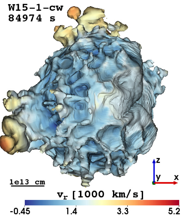
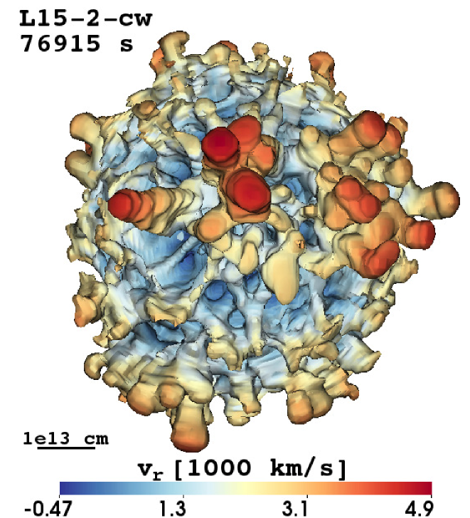
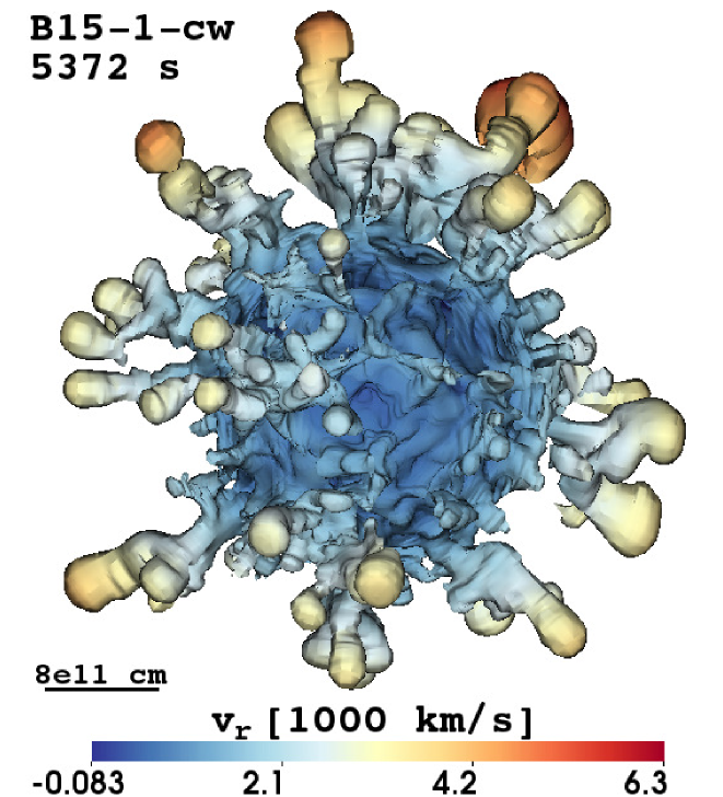
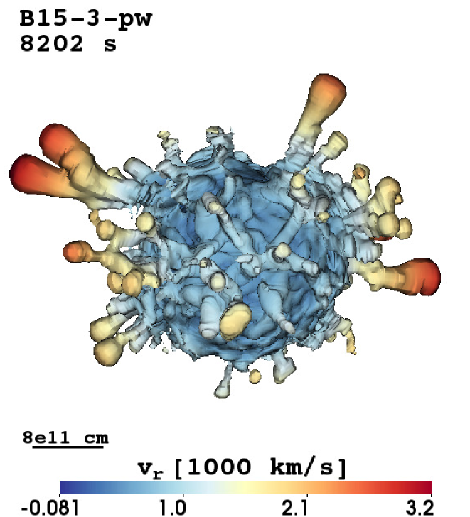
Figure 9: Same as Fig. 7, but for models W15-1-cw, L15-2-cw, B15-1-cw, and B15-3-pw at the shock breakout time.

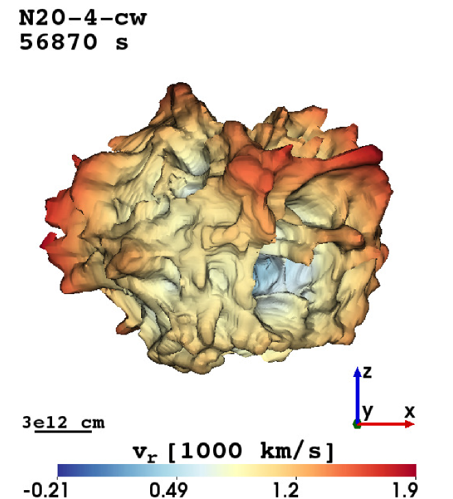
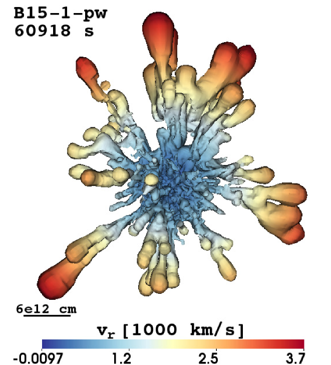
Figure 10: Same as Fig. 7, but for models N20-4-cw and B15-1-pw at 56870 s and 60918 s, respectively.

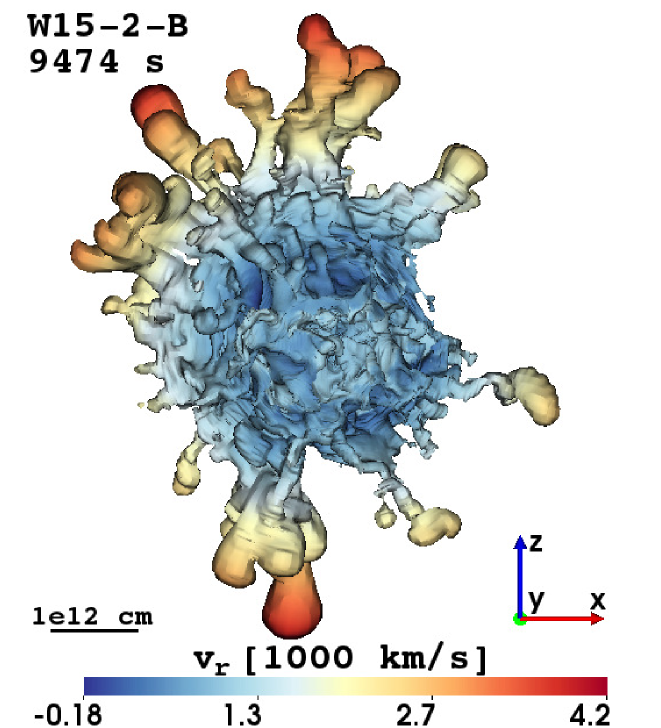
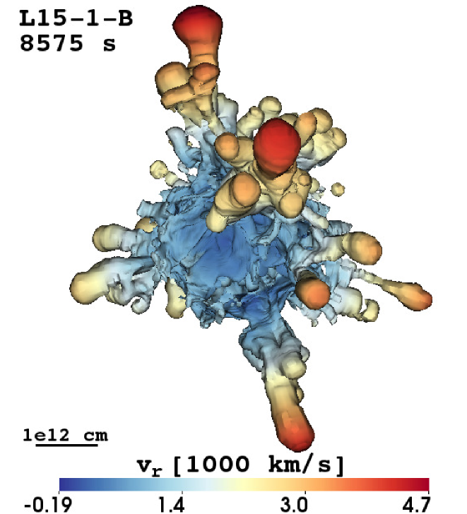
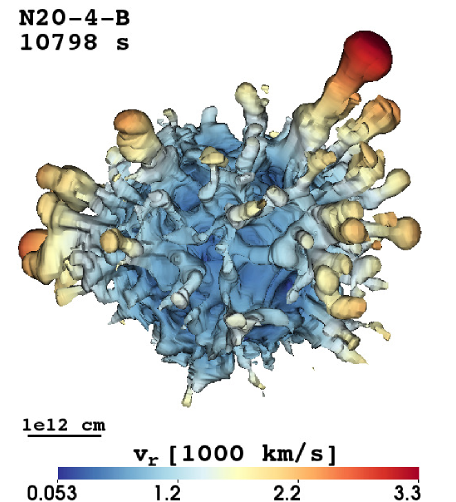
Figure 11: Same as Fig. 7, but for the additional 3D models W15-2-B, L15-1-B, and N20-4-B, discussed in Sect. 5.4.

The morphology of the iron/nickel-rich ejecta of model B15-1-pw differs distinctly and visibly from that of the other three models at shock breakout time. Because a fraction of the iron/nickel-rich ejecta can avoid deceleration by the reverse shock the ejecta separate into two components: a fast component that was able to avoid the reverse shock, and a second, slower one that was drastically slowed down by it. The fast component evolves into elongated RT fingers stretching very far into the hydrogen envelope and experiencing almost no further deceleration. The slower component constitutes the spherical central part of the ejecta expanding at much lower velocities than the fast component.

5.3.4 Dependence on explosion energy

The models shown in Fig. 7, one for each considered progenitor model, have almost the same explosion energy. This fact does not imply, however, a restriction concerning our discussion of the iron/nickel-rich ejecta morphology, because the explosion energy is not responsible for the differences we described above. To prove this statement, we show in Fig. 9 the morphology of the iron/nickel-rich ejecta of models W15-1-cw, L15-2-cw, B15-1-cw, and B15-3-pw at the time of shock breakout. Despite having the highest explosion energy of all calculated models the iron/nickel-rich ejecta in model L15-2-cw are still trapped completely by the reverse shock. Moreover, model B15-3-pw, which possesses the lowest explosion energy of all models, yields the same type of morphology of the iron/nickel-rich ejecta as model B15-1-pw, because the fast iron/nickel-rich RT filaments avoid a strong deceleration by the reverse shock in both models.

Increasing the explosion energy results in a faster propagation of the iron/nickel-rich ejecta, but also gives rise to a faster SN shock, i.e., the relative velocity between the shock and the iron/nickel-rich ejecta, which is the most crucial factor determining whether or not the iron/nickel-rich ejecta will be strongly decelerated by the reverse shock, does not change. We further note that although the iron/nickel-rich ejecta show a lesser degree of global asymmetry in model L15-2-cw than in model L15-1-cw, they evolve in a very similar manner. The asymmetry is less in model L15-2-cw because it explodes faster, which results in a more spherically symmetric distribution of iron/nickel-rich hot bubbles. We also tested whether the fundamental features of radial mixing depend on the seed perturbation pattern imposed during the explosion phase. A comparison of the results of models W15-1-cw and W15-2-cw shows that this is not the case (see Figs. 7 and 9). However, we find interesting differences: $v_{\textrm{max}}(\textrm{Ni})$ varies by up to 20% among the models, while $\langle v\rangle_{1\%}(\textrm{Ni})$ is similar for all models.

5.3.5 Dependence on progenitor star

To be able to discuss possible differences between the morphology of the iron/nickel-rich ejecta of the RSG and BSG models at the time of shock breakout in the RSG progenitors, we had to evolve the BSG models until approximately 60000 s, which is about a factor of ten beyond the time of shock breakout in the BSG models. Fig. 10 displays the morphology of the iron/nickel-rich ejecta of the BSG models N20-4-cw and B15-1-pw at 56870 s and 60918 s, respectively. After the SN shock has crossed the surface of the progenitor star, instabilities continue to grow in model N20-4-cw and the morphology of the iron/nickel-rich ejecta remains no longer smooth and roundish. Narrow spikes/walls of iron/nickel-rich matter stretch in radial direction and further fragmentation of the overall ejecta structure occurs. On the other hand, in our second BSG model B15-1-pw the elongated fingers containing iron/nickel-rich matter grow significantly in length. They even reaccelerate from $\leavevmode\nobreak\ 3300\,$km s^-1 at shock breakout to $\leavevmode\nobreak\ 3700\,$km s^-1 at 61 000 s, but the angular extent and the orientation of these fingers remain unchanged.

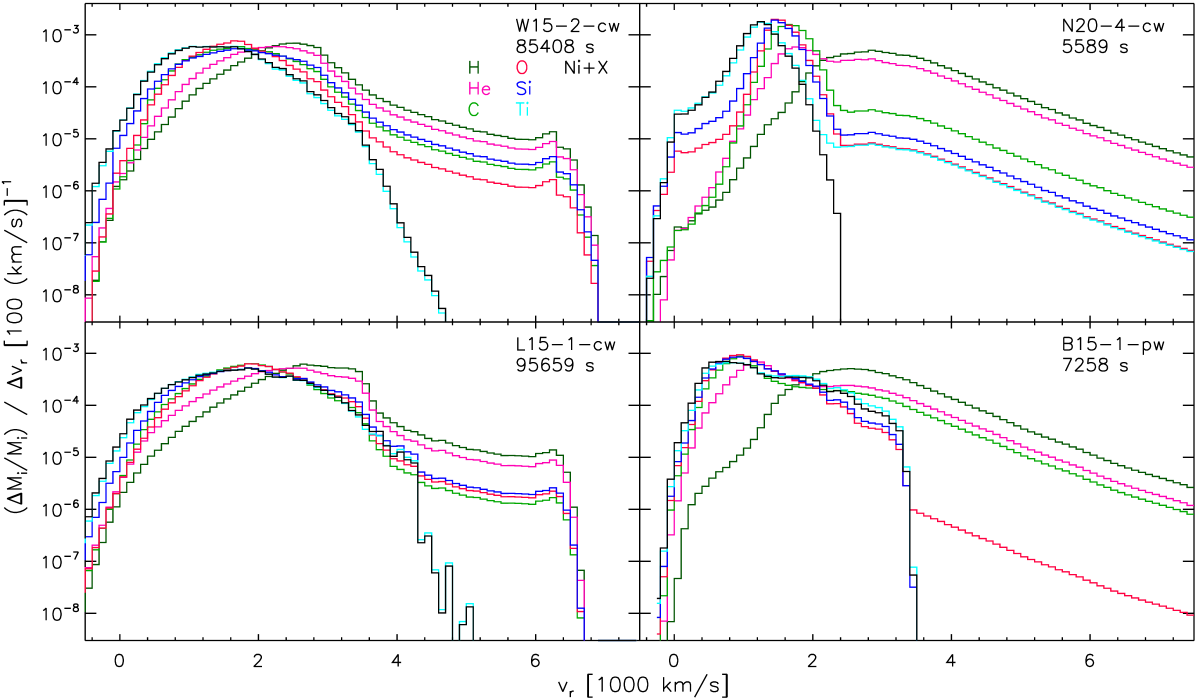
Figure 12: Normalized mass distributions of hydrogen (dark green), helium (magenta), carbon (green), oxygen (red), silicon (blue), titanium (cyan), and “nickel” (black) versus radial velocity for models W15-2-cw (top left), L15-1-cw (bottom left), N20-4-cw (top right), and B15-1-pw (bottom right) at the shock breakout time. The radial velocity bins $\Delta v_{r}$ are 100 km s^-1 wide, and the normalized mass is given per velocity bin.

5.4 Additional 3D models

We have seen that the structure of the B15 progenitor provides favorable conditions for the iron/nickel-rich ejecta to escape a deceleration by the reverse shock at the He/H interface. The shallow density gradient (steep rise of $\rho r^{3}$) inside the He layer and the large width of the He layer of the B15 progenitor cause a strong deceleration of the SN shock while it propagates through the layer. This reduces the velocity difference between the shock and the iron-group ejecta allowing the latter to stay close behind the shock. Moreover, the shallow density gradient encountered at the He/H interface results only in brief and slight acceleration of the SN shock, i.e., the relative velocity between shock and ejecta does not increase by much.

To elaborate on the importance of the progenitor structure we performed three additional 3D simulations, W15-2-B, L15-1-B, and N20-4-B, which were initialized using the 3D explosion models W15-2, L15-1, and N20-4, respectively. The numerical setup of these models was identical to that of models W15-2-cw, L15-1-cw, and N20-4-cw, except for one important difference. Instead of extending the 3D explosion models to the stellar surface using the data from the corresponding progenitor model, we initialized the pre-shock state of models W15-2-B, L15-1-B, and N20-4-B using the data from the B15 progenitor model. Therefore, these models are hybrid models of W15-2, L15-1, and N20-4 explosions inside the B15 progenitor envelope, which allow us to demonstrate the effect of the envelope structure outside of the C+O core on the ejecta morphology. We mapped the hybrid models W15-2-B and N20-4-B at $t_{\mathrm{map}}=1.3\,$s and model L15-1-B at $t_{\mathrm{map}}=1.4\,$s, i.e., at the same times as the corresponding models W15-2-cw, N20-4-cw, and L15-1-cw, respectively (see Table 1). At the time of mapping the SN shock still resides in the C+O core, but is already close to the C+O/He interface of the progenitor star.

Fig. 11 shows the iron/nickel-rich ejecta morphologies of the hybrid models W15-2-B, L15-1-B, and N20-4-B at the end of the simulations using the same rendering technique as in Fig. 7. The evolution of these three models resembles that of the other B15 models qualitatively (see Sect. 5.1, 5.2, and 5.3). The SN shock speeds up and slows down depending on the $\rho r^{3}$ profile as discussed in Section 5.2, and the morphology of the ejecta evolves similarly to that of model B15-1-pw described in Section 5.3. Thus, we refrain from repeating the details here.

It is quite evident from the morphology of the iron/nickel-rich ejecta displayed in Fig. 11 that basic features of the explosion asymmetries seen in model B15-1-pw are also found in all other models exploding inside the B15 progenitor envelope. Fast iron/nickel-rich filaments emerging from the largest bubble of neutrino-heated matter at the time of mapping can escape strong deceleration by the reverse shock at the base of the helium wall and move unhamperedly through the hydrogen envelope. More importantly, the morphologies of the iron/nickel-rich ejecta in the hybrid models are very different from those of models W15-2-cw, L15-1-cw, and N20-4-cw, respectively. This difference goes back to the substitution of the outer structure (i.e., the He and H envelope) of the progenitor models W15, L15, and N20 by that of the progenitor model B15. It is remarkable that in all cases the biggest and strongest plumes created by the neutrino-driven mechanism are the seeds of the longest and most prominent Ni fingers at late stages.

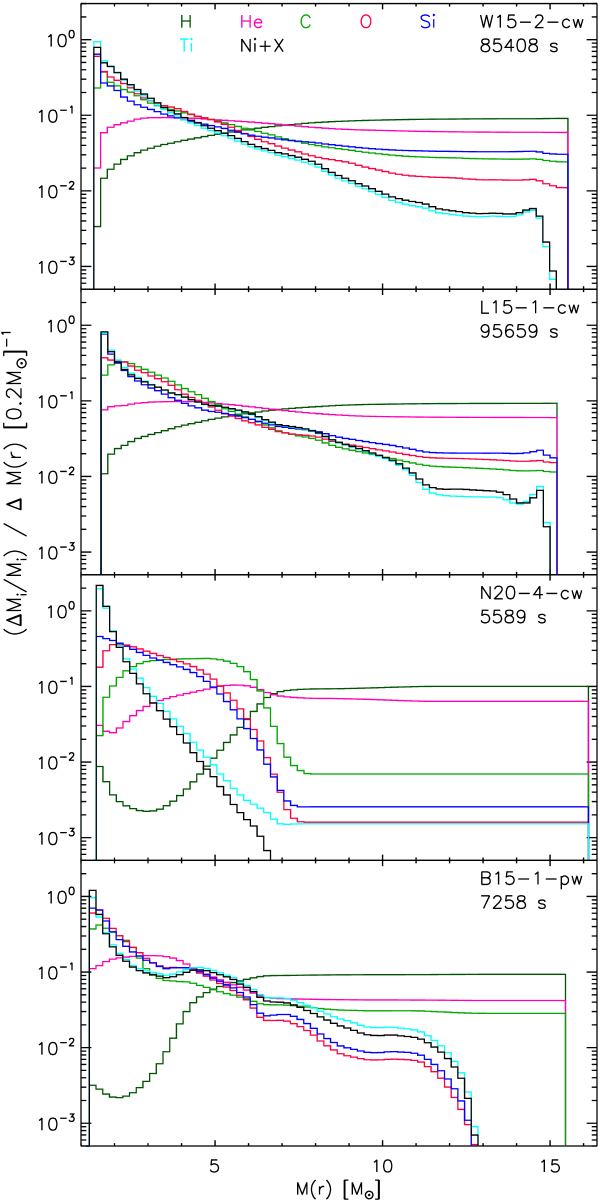
Figure 13: Same as Fig. 12 but versus mass coordinate. The normalized mass is given per mass bin of 0.2 $M_{\odot}$.

5.5 Radial mixing

Figures 12 and 13 display the normalized mass distributions of hydrogen, helium, carbon, oxygen, silicon, titanium, and nickel plus the “tracer” nucleus for models W15-2-cw, L15-1-cw, N20-4-cw, and B15-1-pw as functions of radial velocity and mass coordinate , respectively. The figures show the distributions at the time of shock breakout, i.e., at the time when the minimum (angle-dependent) shock radius exceeds $R_{\ast}$. When interpreting these figures one should keep in mind that the distributions at high velocities and large mass coordinates just reflect the initial composition of the progenitor star.

The heavy ejecta (i.e., the metals) of our RSG models (W15 and L15) are at first compressed into a thin shell once the SN shock begins to decelerate in the hydrogen envelope, and then they are mixed in radial direction due to the growth of RT instabilities at the He/H interface. The resulting distributions of the metals versus radial velocity are of similar shape at the time of shock breakout. They are characterized by a broad maximum centered around a radial velocity of $\approx 2000$ km s^-1 and a high velocity wing extending up to $\approx 6500$ km s^-1 (Fig. 12, left panels). The maximum velocity of ”nickel” is $4200\,$km s^-1 in model W15-2-cw, and $4780\,$km s^-1 in model L15-1-cw (see $v_{\mathrm{max}}$ in Table 2). The matter (mostly H and He, and some C, O, and Si) having even higher velocities represents the rapidly expanding unmixed outer part of the hydrogen envelope. The velocity distribution of the heavy ejecta corresponds to a radial mixing in mass coordinate that comprises almost the whole hydrogen envelope (Fig. 13, top two panels). Figures 12 and 13 further show that some hydrogen (and helium) is mixed down to velocities below $1000$ km s^-1, i.e., into the innermost 2 $M_{\odot}$ of the ejecta.

The amount of both the outward mixing of metals into the hydrogen envelope and the inward mixing of hydrogen into innermost mass layers is much less in the BSG models than in the RSG models. The amount of mixing also differs strongly among the simulated BSG models. The metal distributions are narrower in radial velocity space compared to the corresponding ones of the RSG models. In model N20-4-cw the metal distributions peak at 1500 km s^-1, while the maxima of the metal distributions are located at around 1000 km s^-1 in model B15-1-pw (Fig. 12, right panels). The distributions of the latter model also show a pronounced high velocity shoulder extending to 3400 km s^-1 (Fig. 12, bottom right), while no metal ejecta from the deep core move at velocities higher than 2400 km s^-1 in model N20-4-cw (Fig. 12, top right). We note again that the matter having higher velocities represents the rapidly expanding unmixed outer part of the hydrogen envelope. The velocity distributions of model N20-4-cw correspond to a radial mixing of the lighter metals C, O, and Si out to a mass coordinate of about 7.5 $M_{\odot}$, and of Ti and Ni+X to about 6.7 $M_{\odot}$ (Fig. 13, 3rd panel from top). In model B15-1-pw, all metal ejecta are mixed out to a mass coordinate of $\approx 13\,M_{\odot}$ (Fig. 13, bottom panel). Hydrogen is mixed less deeply into the metal core in the BSG models than in the RSG ones, so that there is no significant amount of hydrogen at velocities lower than 1000 km s^-1, except for a low-velocity tail down to 500 km s^-1 in model B15-1-pw (Fig. 12, bottom right).

The particular shape of the velocity distribution of the metal ejecta in model B15-1-pw (Fig. 12, bottom right) results from the two-component ejecta morphology that is imprinted by the B15 progenitor structure (see discussion in Sect. 5.3). The peak in the metal distributions at low velocities is associated with the ejecta that are decelerated by the reverse shock, while the broad high-velocity shoulder results from the elongated fingers that escaped the reverse shock. These elongated fingers are responsible for the mixing of metals up to an enclosed mass coordinate of about 13 $M_{\odot}$.

5.6 Element distributions

Figure 12, which shows the element distributions as functions of radial velocity, provides no (direct) spatial information and Fig. 13, which gives the element distributions as functions of enclosed mass, contains only 1D information about the spatial (radial) distribution. In addition, using the enclosed mass at a given radius as a radial coordinate becomes questionable when the departure of the mass distribution from spherical symmetry is large. Hence, we sought for a visualization method that incorporates mass, velocity, and spatial information into a single plot. We opted for a method using a set of particles for each chemical element, where the particles are distributed according to the mass distribution of the considered element, and colored each particle by the radial velocity at the particle’s position, which is obtained from the 3D simulation data.

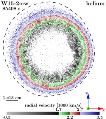
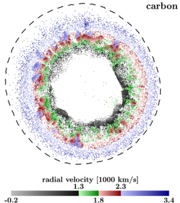
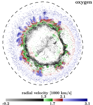
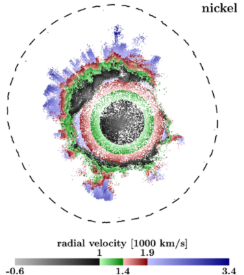
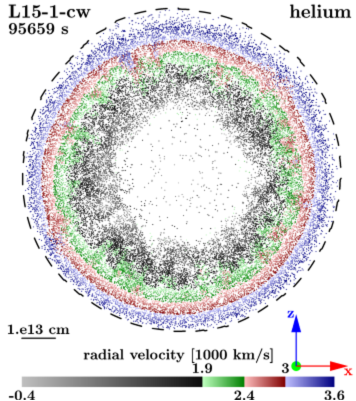
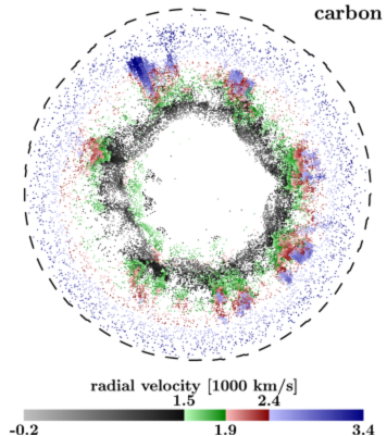
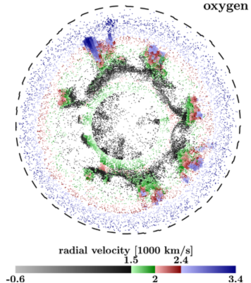
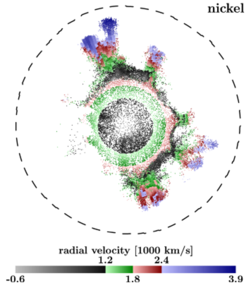
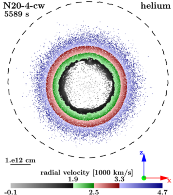
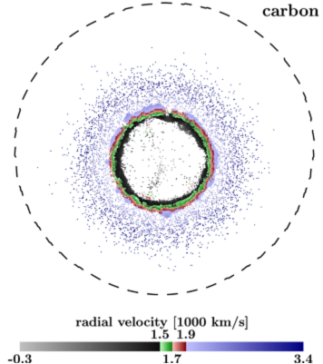
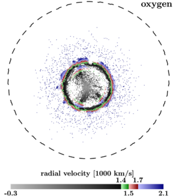
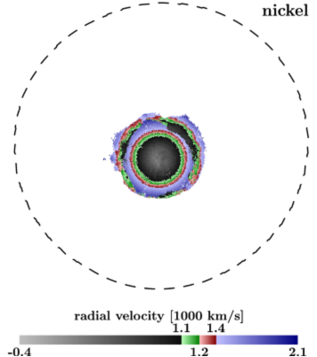
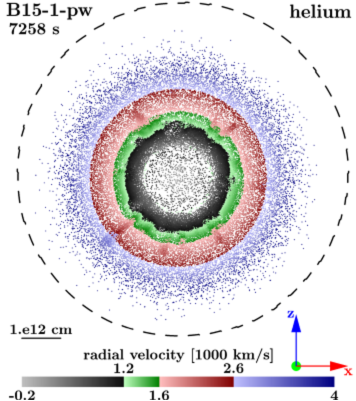
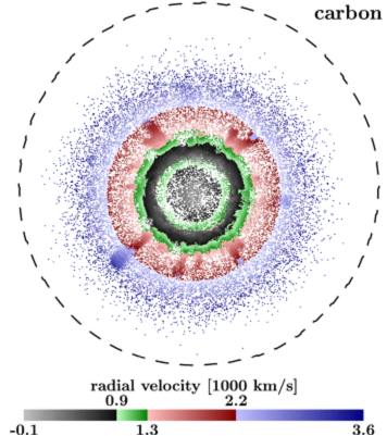
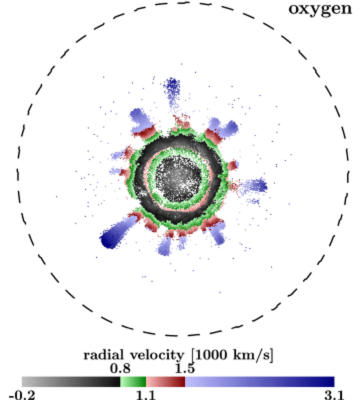
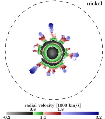
Figure 14: Particle representations of the spatial distributions of He, C, O, and Ni+X for models W15-2-cw, L15-1-cw, N20-4-cw, and B15-1-pw (from top) at the time of shock breakout. We show only particles within a slab given by $-0.05R_{\mathrm{s}}^{\mathrm{max}}\leq y\leq 0.05R_{\mathrm{s}}^{\mathrm{max}}$. The dashed lines give the shock’s location in the $y=0$ plane. The particles are colored according to their radial velocity, which is binned into four bins, each bin containing 25% of the total mass of the element. Blackish particles represent the slowest 25% by mass of an element, while bluish particles mark the fastest 25%. The black thin shell contains matter that was hit by the reverse shock, and thus moves slower than matter located inside this shell (reddish and greenish particles). The positive y-axis points away from the viewer.

We first calculate the number of particles of species $i$ having a radial velocity in the interval $[v_{\mathrm{r}},v_{\mathrm{r}}+\Delta v_{\mathrm{r}})$ by

$$N_{v,i}(v_{\mathrm{r}})=N_{\mathrm{tot},i}\,\frac{\Delta M_{i}(v_{\mathrm{r}})}{M_{i}}$$ (11)

where $N_{\mathrm{tot},i}$ is the total number of particles of species $i$, $\Delta M_{i}(v_{\mathrm{r}})$ is the amount of mass of species $i$ having a radial velocity in the range $[v_{\mathrm{r}},v_{\mathrm{r}}+\Delta v_{\mathrm{r}})$, and $M_{i}$ is the species’ total mass. Then we determine in which grid cell a particle $n$ resides. The probability of a particle having a radial velocity in the range $[v_{\mathrm{r}},v_{\mathrm{r}}+\Delta v_{\mathrm{r}})$ and residing in a grid cell $G$ is

$$\mathcal{P}_{G,i}=\frac{\Delta m_{i}(v_{\mathrm{r}})}{\Delta M_{i}(v_{\mathrm{r}})},$$ (12)

where $\Delta m_{i}(v_{\mathrm{r}})$ is the mass of the species $i$ in the grid cell $G$ having a radial velocity in the range $[v_{\mathrm{r}},v_{\mathrm{r}}+\Delta v_{\mathrm{r}})$. Using a set of uniformly distributed random numbers $\mathcal{R}_{1}$, we determine the grid cell $G$ the particle $n$ is to be assigned to. Knowing the grid cell $G$, where particle $n$ resides, we can calculate the coordinates $(r_{n},\theta_{n},\phi_{n})$ of particle $n$ as

$$r_{n} = r^{L}_{G}+\mathcal{R}_{2}(n)\cdot\Delta r_{G},$$ (13)

$$\theta_{n} = \theta^{L}_{G}+\mathcal{R}_{3}(n)\cdot\Delta\theta_{G},$$ (14)

$$\phi_{n} = \phi^{L}_{G}+\mathcal{R}_{4}(n)\cdot\Delta\phi_{G},$$ (15)

where $r^{L}_{G}$, $\theta^{L}_{G}$, and $\phi^{L}_{G}$ are the coordinates of the left interface of the grid cell $G$, and $\Delta r_{G}$, $\Delta\theta_{G}$, and $\Delta\phi_{G}$ are the sizes of the grid cell in $(r,\theta,\phi)$ direction. Note that we used three additional sets of uniformly distributed random numbers, $\mathcal{R}_{2}$, $\mathcal{R}_{3}$, and $\mathcal{R}_{4}$, in calculating the coordinates of the particle. The particle’s radial velocity is given by the radial velocity of grid cell $G$.

We binned the radial velocities into four bins (not to be confused with the velocity intervals discussed above!), each bin containing 25% of the total mass of an element. To provide some qualitative information of the mass distribution at a glance, we used different color gamuts to show the variation of the velocity within each bin. Because each color gamut contains 25% of the total mass of a species, blackish particles represent the slowest 25% by mass of a species, while blueish particles mark the fastest 25% (see Figs. 14 and 15).

Fig. 14 displays a slab of the particle distributions of helium, carbon, oxygen, and nickel (including the tracer $X$) for models W15-2-cw, L15-1-cw, N20-4-cw, and B15-1-pw. The slab is defined by $-0.05R_{\mathrm{s}}^{\mathrm{max}}\leq y\leq 0.05R_{\mathrm{s}}^{\mathrm{max}}$, where $R_{\mathrm{s}}^{\mathrm{max}}$ is the maximum radius of the SN shock. In all models, the helium distributions are almost spherically symmetric with only slight imprints of asymmetries, while the distributions of the metals show pronounced asymmetries.

A comparison of the distributions of carbon and oxygen between RSG and BSG models is particularly interesting. In the RSG models the ejecta that were compressed by the reverse shock (forming after the SN shock had crossed the He/H interface) are strongly fragmented by RT instabilities. As a result both the carbon and oxygen shell are strongly distorted. This situation contrasts with that in the BSG models, in particular model N20-4-cw, where carbon and oxygen retain a more coherent spherical shell structure because of a less vigorous and less long-lasting growth of RT instabilities at the C/O/He and He/H interfaces in the BSG progenitors in comparison with the RSG progenitors. To confirm that no significant fragmentation of the carbon shell occurs in the BSG models we show in Fig. 15 the carbon distribution of models N20-4-cw and B15-1-pw at 56870 s and 60918 s, respectively, i.e., at a time when mixing seems to have ceased. We used here the same visualization technique as in Fig. 14, but the slab is defined by $-2\times 10^{12}\,\mathrm{cm}\leq y\leq 2\times 10^{12}\,\mathrm{cm}$, and only particles residing inside a radius of $4\times 10^{13}$ cm are shown.

In model B15-1-pw the spherical distributions of carbon and oxygen are superimposed by asymmetries produced by elongated RT fingers of ejecta which escaped the reverse shock below the He/H interface. Figure 14 implies that more than 50% of the nickel mass of this model is carried by the elongated structures (fingers) with velocities larger than approximately $1100\,$km s^-1 (red and blue particles in the bottom right panel).

The spatial locations of the He and metal ejecta (i.e., He, C, O, and Ni+X) also differ between RSG and BSG models (Fig. 14). In the former ones they are mixed outward close to the SN shock, while they stay far behind the shock in the BSG models. This even holds for model B15-1-pw with its fast-moving RT fingers that escaped the interaction with the reverse shock.

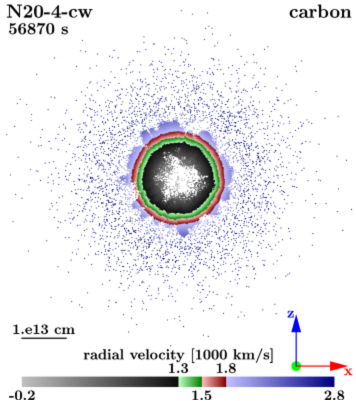
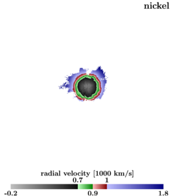
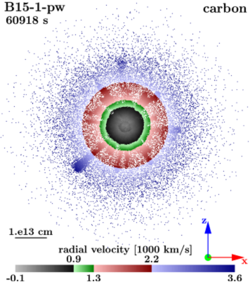
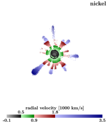
Figure 15: Same as Fig. 14 but displaying only those particles that reside inside a sphere of radius $4\times 10^{13}$ cm and within a slab given by $-2\times 10^{12}\,\mathrm{cm}\leq y\leq 2\times 10^{12}\,\mathrm{cm}$ for models N20-4-cw (top) and B15-1-pw (bottom) at 56870 s and 60918 s, respectively.

6 Conclusions

We have presented the results of three-dimensional hydrodynamic simulations of core collapse supernovae comprising the evolution of the shock wave and of the neutrino-heated metal-rich ejecta from shock revival to shock breakout in four different progenitor stars: two 15 $M_{\odot}$ RSG, a 20 $M_{\odot}$ BSG, and a 15 $M_{\odot}$ BSG. The simulations were initialized from a subset of the 3D explosion models of Wongwathanarat et al. (2010b, 2013), which cover the evolution from about 10 ms up to 1.4 s after core bounce. The explosions in these models were initiated by imposing suitable values for neutrino luminosities and mean energies at the inner grid boundary located at a finite, time-dependent radius. Neutrino transport and neutrino-matter interactions were treated by the ray-by-ray gray neutrino transport scheme of Scheck et al. (2006) including a slight modification of the prescription for neutrino mean energies at the inner grid boundary (Ugliano et al. 2012).

At the end of the initial explosion simulations the SN shock had reached a radius of $10^{9}$ to 2$\times 10^{9}$ cm, i.e., it still resided inside the C+O core of the progenitor star. Combining the (early-time) 3D explosion models of Wongwathanarat et al. (2013) with the late-time 3D runs presented here allowed us to study the evolution of CCSN and their ejecta for a set of progenitor models (and not just for one case as in HJM10) in 3D for the first time from shortly ($\approx 10\,$ms) after core bounce until many hours later.

To aid us with the analysis of the 3D simulations, we have also calculated the linear Rayleigh-Taylor growth rates of 1D explosion simulations performed with the angle-averaged (early-time) 3D explosion models, which provide a qualitatively good criterion for the expected growth in different layers of the progenitor star. The growth factors are large near the C+O/He and He/H interfaces, which is expected from the density profiles of the progenitor stars that vary strongly at these interfaces in all models.

We compared our simulations performed with the Yin-Yang grid to those of Hammer et al. (2010) and find good agreement concerning the amount and extent of mixing and the ejecta morphologies, except that the peak radial velocity of nickel is roughly 10% slower and that the slowest hydrogen moves slightly faster in our models. We attribute these differences to the numerical resolution, which was slightly higher in the Hammer et al. (2010) models in polar regions. The results of two specific 3D simulations, which we performed with 1^∘ and 2^∘ angular resolution, suggest that an angular resolution of 2^∘ is sufficient for our goals, but lower angular resolution tends to cause the mentioned velocity differences. Our primary intention was neither to determine details of the small-scale structure nor the precise peak velocities of the ejecta, but to study the dependence of the ejecta morphology on explosion energy and the progenitor.

Our simulations show that the evolution of the SN shock and the neutrino-heated ejecta within the stellar envelope is complex, involving several types of hydrodynamic instabilities. After crossing a composition interface, the deceleration of the SN shock leads to the formation of RT unstable dense shells and the formation of a strong reverse shock in the case of the He/H interface. The neutrino-heated ejecta propagating at some distance behind the SN shock may penetrate these dense shells causing large-amplitude perturbations there, if they are fast enough to catch up with the shell. Whether or not an interaction occurs between the reverse shock (propagating inward in mass) and the fastest fraction of the iron-nickel-rich ejecta is determined by the velocity of the latter relative to the SN shock.

We find that the relative velocity depends in turn on three important features of the density profile of the progenitor star: the compactness of the C+O core, the density structure of the helium shell, and the density gradient at the He/H interface. We confirmed this fact by performing three additional 3D simulations where we replaced the outer C/O core, the helium and hydrogen shell of the two RSG progenitors and of the 20 $M_{\odot}$ BSG progenitor by that of the 15 $M_{\odot}$ BSG progenitor. These 3D simulations demonstrated: (i) the iron/nickel-rich plumes do not have enough time to grow into finger-like structures before they are slowed down by the reverse shock in the more compact BSG stars because of the earlier onset of SN shock deceleration and reverse shock formation, and (ii) both a shallow density profile inside the helium shell and a small density decrease at the He/H interface reduce the relative velocity between the ejecta and the SN shock, and hence help the fastest iron/nickel-rich ejecta to avoid the interaction with the reverse shock.

Considering the results of our 3D simulations performed with four different progenitor stars, we can categorize the morphology of the iron/nickel-rich ejecta hours after the onset of the explosion into three types.

For RSG progenitors (W15 and L15), the late time morphology of the iron/nickel-rich ejecta is characterized by small RT fingers bunched together into a few groups whose angular positions agree with those of the few largest, fast-rising plumes of neutrino-heated ejecta, which were generated by hydrodynamic instabilities during the shock revival phase. This type of ejecta morphology is mainly due to the strong acceleration of the SN shock at the He/H interface and its subsequent even stronger deceleration inside the H envelope of the RSG progenitors. The decelerating SN shock gives rise to a strongly RT unstable stratification near the interface and the formation of a strong reverse shock, while the acceleration of the SN shock increases the spatial separation of SN shock and iron-nickel-rich ejecta. The latter fact also implies that the distance between the reverse shock and the ejecta is relatively large in the RSG models, i.e., there is more time for the fast plumes of iron/nickel-rich ejecta to grow into extended fingers before they eventually are decelerated by the reverse shock.

The second type of morphology is produced by models based on the N20 progenitor star, where the iron/nickel-rich ejecta can be described by fragmented roundish structures, which are the result of two facts. Firstly, the iron/nickel-rich ejecta propagate with a lower velocity than the SN shock. Secondly, the only moderate drop of the density in this model at the He/H interface causes the SN shock not to accelerate much at this interface. The combination of both facts implies little time for large non-spherical deformations of the iron/nickel-rich ejecta to develop before they are compressed by the reverse shock, which forms ahead of the ejecta near the He/H interface.

Models based on the B15 progenitor star exhibit a third type of morphology. The iron/nickel-rich ejecta appear as a few, very distinct elongated RT fingers penetrating quite large distances into the fast-moving hydrogen envelope. These stretched RT fingers are those parts of the iron/nickel-rich ejecta that propagated fast enough to avoid a deceleration by the reverse shock. This was possible for this progenitor, because the SN shock experienced a strong deceleration inside its helium shell and only a small acceleration at its He/H interface.

For all simulated models, except the one based on the N20 progenitor, we find that there is a clear correlation between the asymmetries of the iron/nickel-rich ejecta at late times and the early-time asymmetries resulting from hydrodynamic instabilities generated during the onset of the SN explosion. However, this is not too surprising, because the growth of RT instabilities at composition interfaces in our simulations is in fact seeded by large-scale, large-amplitude perturbations caused by the blast asymmetries at early times rather than by small-scale random perturbations. The latter perturbations were used in simulations which cover the first second of the SN explosion assuming spherical symmetry. On the other hand, in the simulated model based on the N20 progenitor, the early-time, large-scale asymmetries of the iron/nickel-rich ejecta are greatly diminished by the interaction between the ejecta and the reverse shock occurring already in the helium shell of the star. Thus, the iron/nickel-rich ejecta lose memory of the early-time asymmetries, i.e., we find no clear correlation of late-time and early-time asymmetries of the iron/nickel-rich ejecta for this progenitor.

Concerning the maximum velocities of the iron/nickel-rich ejecta we find that these vary between 3700 and 4400 km s^-1 in our RSG models, while they do not exceed 2200 km s^-1 in our 20 solar mass BSG model and 3400 km s^-1 in our 15 solar mass BSG model.

Hydrogen is mixed less deeply into the metal core in the BSG models than in the RSG ones so that there is no significant amount of hydrogen at a velocity lower than 1000 km s^-1 in the BSG models, except for a low-velocity tail down to 500 km s^-1 in the model based on the B15 BSG progenitor. This difference between BSG and RSG progenitors can be understood from the growth rates of the RT instabilities, which are larger in RSG progenitors because these progenitors possess a steeper density gradient at the H/He interface than BSG progenitors, giving rise to a more strongly RT unstable layer after the passage of the SN shock. Hence, there will be more and more extended mixing of hydrogen into the inner parts of the ejecta, i.e., to lower velocities, in RSG progenitors.

In our 3D explosion models, we seeded the initial development of nonradial instabilities in the SN core in the neutrino-heated region by small (0.1%) random (velocity) perturbations on the grid scale. Hence, we ignored the possible existence of larger-scale and larger-amplitude inhomogeneities in the progenitor core before the onset of the collapse, which may arise due to vigorous convection during pre-collapse oxygen and/or silicon burning (Arnett & Meakin 2011). Corresponding nonradial mass motions could affect explosion asymmetries, neutron-star kicks, and nickel mixing before core collapse as well as during the explosion. In addition, Couch & Ott (2013) showed that the revival of the stalled supernova shock by neutrino heating could be triggered by nonradial flows in the progenitor core, because perturbations in the Si/O burning shells, when advected through the accretion shock, enhance nonradial mass motions and turbulent pressure in the postshock region (Couch & Ott 2014; Müller & Janka 2014). While such effects might be of relevance in the context discussed in our paper, it is unclear whether the relatively large initial perturbations that are needed to make a sizable impact are realistic (Müller & Janka 2014). A quantitatively meaningful assessment is currently not possible because the perturbation pattern and amplitude in 3D stars prior to core collapse must still be determined by multi-dimensional simulations of the late stages of stellar evolution.

Concerning the final ejecta morphology of the supernova remnant, there are two further potentially important effects that are not covere by our present simulations. Firstly, RT instabilities will occur at the interface separating matter in the shocked stellar envelope from shocked circumstellar matter after shock breakout (Gawryszczak et al. 2010). This interface becomes RT unstable when the supernova shock is decelerating in the circumstellar matter, i.e., when the less dense circumstellar matter is moving slower than the shocked and denser matter of the stellar envelope ejected in the SN (Chevalier et al. 1992). Secondly, the energy release by the radioactive decay of nickel into cobalt and iron can cause local heating of the ejecta, which can modify the ejecta morphology. The actual importance of both effects can only be clarified by extending our simulations to much later times, which we plan to do next.