Fractal analysis of the galaxy distribution in the redshift range $0.45\leq z\leq 5.0$

Abstract

This paper performs a fractal analysis of the galaxy distribution and presents evidence that it can be described as a fractal system within the redshift range of the FORS Deep Field (FDF) galaxy survey data. The fractal dimension $D$ was derived by means of the galaxy number densities calculated by Iribarrem et al. (2012a) using the FDF luminosity function parameters and absolute magnitudes obtained by Gabasch et al. (2004, 2006) in the spatially homogeneous standard cosmological model with $\Omega_{m_{0}}=0.3$, $\Omega_{\Lambda_{0}}=0.7$ and $H_{0}=70\;\mbox{km}\;{\mbox{s}}^{-1}\;{\mbox{Mpc}}^{-1}$. Under the supposition that the galaxy distribution forms a fractal system, the ratio between the differential and integral number densities $\gamma$ and $\gamma^{\ast}$ obtained from the red and blue FDF galaxies provides a direct method to estimate $D$ and implies that $\gamma$ and $\gamma^{\ast}$ vary as power-laws with the cosmological distances, feature which provides a second method for calculating $D$. The luminosity distance $d_{\scriptscriptstyle L}\,$, galaxy area distance $d_{\scriptscriptstyle G}$ and redshift distance $d_{z}$ were plotted against their respective number densities to calculate $D$ by linear fitting. It was found that the FDF galaxy distribution is better characterized by two single fractal dimensions at successive distance ranges, that is, two scaling ranges in the fractal dimension. Two straight lines were fitted to the data, whose slopes change at $z\approx 1.3$ or $z\approx 1.9$ depending on the chosen cosmological distance. The average fractal dimension calculated using $\gamma^{\ast}$ changes from $\langle D\rangle=1.4^{\scriptscriptstyle+0.7}_{\scriptscriptstyle-0.6}$ to $\langle D\rangle=0.5^{\scriptscriptstyle+1.2}_{\scriptscriptstyle-0.4}$ for all galaxies. Besides, $D$ evolves with $z\,$, decreasing as the redshift increases. Small values of $D$ at high $z$ mean that in the past galaxies and galaxy clusters were distributed much more sparsely and the large-scale structure of the universe was then possibly dominated by voids. The results of Iribarrem et al. (2014) indicating that similar fractal features having $\langle D\rangle=0.6\pm 0.1$ can be found in the 100 $\mu$m and 160 $\mu$m passbands of the far-infrared sources of the Herschel/PACS evolutionary probe (PEP) at $1.5\lesssim z\lesssim 3.2$ are also mentioned.

1 Introduction

Fractal analysis of the galaxy distribution consists of using the standard techniques of fractal geometry to verify whether or not a given galaxy distribution has fractal properties and calculating its key feature, the fractal dimension $D$, with data gathered from the distribution. The fractal dimension quantifies how “broken”, or irregular, is the distribution, that is, how far a distribution departs from regularity. Hence, in the context of the galaxy distribution the fractal dimension is simply a measure of the possible degree of inhomogeneity in the distribution, which can be viewed as a measure of galactic clustering sparsity or, complementarily, the dominance of voids in the large-scale structure of the Universe. Values of $D$ smaller than the corresponding topological dimension where the fractal system is embedded mean a more irregular pattern (Mandelbrot 1983). Systems having three dimensional topology such as the galaxy distribution are regular, or homogeneous, if $D=3$. Accordingly, increasing irregularities, or inhomogeneities, in the distribution corresponds to decreasing values of the fractal dimension, that is, $D<3$ (Ribeiro and Miguelote 1998; Sylos Labini et al. 1998).

Fractal distributions described by one fractal dimension are called single fractals and form the simplest fractal systems. This is, of course, a simplification, but a useful one as a first approach for describing complex distributions or for analyzing simple systems (Ribeiro and Miguelote 1998). More complex distributions can exhibit different values of $D$ at specific distance ranges defined in the distribution, that is, different scaling ranges in the fractal dimension so that $D=D(d)$ where $d$ is the distance. In such a case there is a succession of single fractal systems. An even more complex situation can occur if, for instance, quantities like mass or luminosity range between very different values, i.e., if they possess a distribution. Such variations require a generalization of the fractal dimension in order to include the distribution and, hence, the system is characterized by several fractal dimensions in the same scaling range, that is, a whole spectrum of dimensions whose maximum value corresponds to the single fractal dimension $D$ the system would have if the studied quantity did not range. In such a case the system is said to exhibit a multifractal pattern (Gabrielli et al. 2005).

Cosmological models which describe the galaxy distribution as a fractal system are not new. Several of such studies can be found in the literature, either in the context of Newtonian cosmology (Pietronero 1987; Ribeiro and Miguelote 1998; Sylos Labini et al. 1998; Abdalla et al. 1999; Gabrielli et al. 2005; Sylos Labini 2011; and references therein) or in models based on relativistic cosmology (Ribeiro 1992ab, 1993, 1994, 2001ab, 2005; Abdalla et al. 2001; Abdalla and Chirenti 2004; Mureika and Dyer 2004; Mureika 2007; and references therein). Fractal analyzes based on Newtonian cosmology often perform detailed statistical tests on empirical data, but they are usually limited to very small redshift ranges where inhomogeneities predicted in standard relativistic models are not detectable (Rangel Lemos and Ribeiro 2008). On the other hand, relativistic cosmology fractal models had to cope with fundamental conceptual problems like how to define fractality in a curved spacetime and what is the meaning of observable homogeneity, as opposed to spatial homogeneity (Ribeiro 1992ab, 1995, 2001b, 2005; Rangel Lemos and Ribeiro 1998). Overcoming these difficulties led to mostly theoretical models with little or none empirical data analysis.

Studies not motivated by fractals sometimes provide, nevertheless, data analyzes which can be used to quantitatively measure statistical fractal properties in the galaxy distribution because some of their results suggest a fractal pattern in this distribution. This is the case of Albani et al. (2007; hereafter A07) and, more recently, Iribarrem et al. (2012a, hereafter Ir12a; see also Iribarrem et al. 2014) who carried out relativistic analyzes of galaxy number densities at high redshift ranges based on empirical data derived from the galaxy luminosity function (LF). A07 used LF data from the CNOC2 galaxy redshift survey (Lin et al. 1999) in the range $0.1\leq z\leq 1.0$, whereas Ir12a (see also Iribarrem et al. 2012b) carried out a similar analysis using LF data extracted from red and blue galaxies belonging to the FORS Deep Field (FDF) galaxy redshift survey (Gabasch et al. 2004, 2006; hereafter G04 and G06, respectively) in the range $0.45\leq z\leq 5.0$. Both studies found evidence that at high redshifts the galaxy number densities obtained from the LF scale as power-laws with the relativistic distances. As it is well-known, distributions obeying power-laws strongly suggest fractal behavior (Mandelbrot 1983).

Measuring fractal properties from these data analyzes became possible because the LF was computed using the 1/V_max method, which is a non-parametric estimator that assumes a homogeneous distribution on average to correct for the incompleteness caused by the flux limit of a survey. Subsequent integration over absolute magnitudes produced the selection function, which is essentially a galaxy number density that can be transformed into other densities by using the relativistic cosmology based framework developed by Ribeiro and Stoeger (2003), A07 and Ir12a. Assuming that the LF parameters of G04 and G06 are not biased by any other radial selection effects, then our interest was basically focused on making sure that the number densities obtained by integrating the LF were not biased by the integration limit. By using an absolute magnitude cut based on the formal 50% completeness limit of the I-band, at which the galaxies were selected, Ir12a ended up with a comoving number density that corresponds to the brighter objects of the sample in separate redshift bins. Such subsamples yield approximately the same number density as the one computed straightforwardly from a volume-limited sample. Together with correcting for flux limit incompleteness, done in the building of the LF, keeping under control a possible bias introduced by the redshift dependence of the integration limit is an essential requirement for measuring fractal dimensions.

The aim of this paper is to perform a relativistic analysis of the results presented in Ir12a from a fractal perspective. We focused on this work because it is based on the FDF survey, whose galaxies were measured at several wavebands and out to deep redshift ranges. Although this is a survey that scanned a limited sky area, its redshift depth is the main feature that motivated this work, as having measured galaxies up to $z=5.0$ the FDF survey is capable of producing results that can indicate possible observable inhomogeneities even when one uses the standard spatially homogeneous Friedmann-Lemaître-Robertson-Walker (FLRW) cosmological model and, hence, if a fractal approach for studying the galaxy distribution is worth pursuing with other, less limited, deep samples. In addition, since the results were obtained assuming the FLRW cosmology with $\Omega_{m_{\scriptscriptstyle 0}}=0.3$, $\Omega_{\Lambda_{\scriptscriptstyle 0}}=0.7$ and $H_{0}=70\;\mbox{km}\;{\mbox{s}}^{-1}\;{\mbox{Mpc}}^{-1}$, this means that the cosmological principle will be valid in the whole analysis of this paper. Actually, it has already been shown elsewhere that there is no contradiction whatsoever between observational fractals and the cosmological principle (Ribeiro 2001b, 2005; Rangel Lemos and Ribeiro 2008).

The results show that the simplest fractal description of the galaxy distribution in the redshift range $0.45\leq z\leq 5.0$ needs two fractal dimensions associated to specific distance ranges to describe the distribution. In other words, we found two scaling ranges in the fractal dimension. The transition between these two regions spans the range $z=1.3-1.9$. In the first region, defined at $0.45\leq z\lesssim 1.3-1.9$, the average fractal dimension is $\langle D\rangle\simeq 1-2$. The second region comprises the scale $1.3-1.9\lesssim z\leq 5.0$ where the fractal dimension was found to be $\langle D\rangle<1$. These estimates bring initial confirmation for the theoretical prediction made by Rangel Lemos and Ribeiro (2008) of an evolving fractal dimension, with decreasing values for $D$ as $z$ increases. Small values of $D$ mean a more sparse clustering distribution, which implies that in the past voids may have dominated the large-scale galactic structure. Our results also give preliminary indication that $D$ becomes very small, close to zero, at the outer limits of the FDF survey, a result which implies that either the galaxies belonging to the fractal system are not being observed at large values of $z$ or that the large-scale structure of the universe becomes essentially void dominated. The latter case perhaps implies that the galactic clustering itself could have started at a relatively recent epoch in the evolution of the Universe, when $z<5$. Finally, due to the big uncertainties in the calculated values of $D$, it is clear these results must be seen as preliminary, but even so they may also indicate that the fractal galaxy distribution is possibly better characterized by more than two scaling ranges in the fractal dimension, that is, various successive single fractal systems having several fractal dimensions associated to specific distance ranges.

The plan of the paper is as follows. In Sect. 2 we discuss the tools necessary for the fractal analysis of the galaxy distribution in a relativistic cosmology setting. Sect. 3 briefly summarizes the features of the FDF survey and the methodology employed by Ir12a to extract number densities from the luminosity function built with the FDF galaxies. Sect. 4 presents the results of the fractal analysis and Sect. 5 presents our conclusions.

2 Relativistic fractal cosmology

“Theories crumble, but good observations never fade.”
Harlow Shapley

The idea that there exists a fractal pattern in the matter distribution of the Universe is old, actually several centuries old (Ribeiro 2005, Baryshev and Teerikorpi 2002, Grujić 2011, and references therein). In more recent times, irregularities in the galaxy distribution have been studied by several authors since at least the 1900s, that is, well before fractals were introduced in the literature, as they reasoned that empirical evidence supports the idea that galaxies clump together to form groups of galaxies, which themselves form clusters of galaxies and they then form even larger groups, the galaxy super-clusters, and so on. This was called “the hierarchical organization of galaxies” and models based on this concept were collectively known as hierarchical cosmology (Charlier 1908, 1922; Selety 1922; Einstein 1922; Amoroso Costa 1929; Carpenter 1938; de Vaucouleurs 1960, 1970; Wertz 1970, 1971; Haggerty and Wertz 1972). Fractal ideas were developed much later, but soon after their appearance it became clear that this galactic hierarchical organization amounts to nothing more than assuming a fractal galaxy distribution (Mandelbrot 1983). Those earlier studies were, nevertheless, carried out within the limited scope of the Newtonian cosmology framework, since relativistic hierarchical (fractal) cosmologies appeared even later and had first to overcome conceptual issues like, among others, the meaning of a cosmological fractal dimension in a curved spacetime whose observations are made along the past light cone. It is not the aim of this work to provide a detailed discussion of the conceptual issues surrounding the relativistic approach to fractal cosmology, discussion which can be found elsewhere (Ribeiro 1992ab, 1994, 1995, 2001b, 2005; Rangel Lemos and Ribeiro 2008), although a brief presentation of these conceptual issues can be found in Sect. 2.1 below. So, here we shall mainly restrict ourselves to present the basic tools capable of providing a fractal description of the galaxy distribution in a relativistic cosmology framework.

As discussed above, fractals are characterized by power-laws and, therefore, we must put forward relativistic-based analytical tools capable of capturing fractal features from the empirical data, where the latter are, by definition, collected along the observer’s backward null cone. To elaborate on this point, let us start by writing the defining expression of the differential density $\gamma$ (Wertz 1970, 1971),

$$\gamma=\frac{1}{4\pi{(d)}^{2}}\frac{\mathrm{d}N}{\mathrm{d}(d)},$$ (1)

where $N$ is the cumulative number counts of cosmological sources (galaxies) and $d$ is the observational distance. From this definition it is clear that $\gamma$ gives the rate of growth in number counts, or more exactly in their density, as one moves along the observational distance $d$.

From a relativistic viewpoint, it is well-known that cosmological distances are not uniquely defined (Ellis 1971, 2007) and, therefore, we have to replace $d$ for $d_{i}$ in the equation above, where the index indicates the chosen distance measure. The ones to be used here are the redshift distance $d_{z}$, the luminosity distance $d_{\scriptscriptstyle L}$ and the galaxy area distance $d_{\scriptscriptstyle G}$. The last two are connected by the Etherington reciprocity law (Etherington 1933; Ellis 1971, 2007),

$$d_{\scriptscriptstyle L}=(1+z)\,d_{\scriptscriptstyle G},$$ (2)

where $z$ is the redshift. The redshift distance is defined by the following equation,

$$d_{z}=\frac{c\,z}{H_{0}},$$ (3)

where $c$ is the light speed and $H_{0}$ is the Hubble constant. This definition of $d_{z}$ is, of course, only valid in the FLRW metric. A07 and Ir12a showed that within the FLRW cosmology the densities defined with both $d_{\scriptscriptstyle L}$ and $d_{z}$ have power-law properties and we shall see below that the same is true with $d_{\scriptscriptstyle G}$. Another distance measure that can be defined in this context is the angular diameter distance $d_{\scriptscriptstyle A}$, also known as area distance. However, densities defined with $d_{\scriptscriptstyle A}$ have the odd behavior of increasing as $z$ increases, making it unsuitable to use in the context of a fractal analysis of the galaxy distribution (Ribeiro 2001b, 2005; A07; Rangel Lemos and Ribeiro 2008).

The discussion above about cosmological distances implies that Eq. (1) must be rewritten as follows (Ribeiro 2005),

$$\gamma_{i}=\frac{1}{4\pi{(d_{i})}^{2}}\frac{\mathrm{d}N}{\mathrm{d}(d_{i})}=\frac{\mathrm{d}N}{\mathrm{d}z}{\left[4\pi{(d_{i})}^{2}\frac{\mathrm{d}(d_{i})}{\mathrm{d}z}\right]}^{-1},$$ (4)

where ($i={\scriptstyle G}$, ${\scriptstyle L}$, ${\scriptstyle Z}$) according to the distance definition used to calculate the differential density. Integrating the equation above over an observational volume $V_{i}$ produces the integral density $\gamma_{i}^{\ast}$, which can be written as (Ribeiro 2005),

$$\gamma_{i}^{\ast}=\frac{1}{V_{i}}\int_{V_{i}}\gamma_{i}\,\mathrm{d}V_{i},$$ (5)

where,

$$V_{i}=\frac{4}{3}\pi{(d_{i})}^{3}.$$ (6)

Clearly $\gamma_{i}^{\ast}$ gives the number of sources per unit of observational volume located inside the observer’s past light cone out to a distance $d_{i}$. From its definition it is straightforward to conclude that the following expression holds,

$$\gamma_{i}^{\ast}=\frac{N}{V_{i}}.$$ (7)

One should note that $\gamma$ and $\gamma^{\ast}$ are radial quantities and, therefore, must not be confused with the similar looking functions advanced by Pietronero (1987), the conditional density $\Gamma$ and the integrated conditional density $\Gamma^{\ast}$ (see also Sylos Labini et al. 1998; Gabrielli et al. 2005). The latter two are quantities defined in statistical sense, which means averaging all points against all points, whereas $\gamma$ and $\gamma^{\ast}$ are radial only quantities. Luminosity functions computed from redshift surveys data are presented as radial functions, so one should use radial densities with LF derived data.

The key hypothesis behind the assumption that the smoothed-out galaxy distribution forms a single fractal system can be translated into a simple equation relating the cumulative number counts of observed cosmological sources $[N]_{{\textstyle{\scriptscriptstyle\rm obs}}}$ and the observational distances $d_{i}$. This is the number-distance relation, whose expression may be written as,

$$[N]_{{\textstyle{\scriptscriptstyle\rm obs}}}=B\,{(d_{i})}^{D},$$ (8)

where $B$ is a positive constant and $D$ is the fractal dimension. This expression is the keystone of the Pietronero-Wertz hierarchical (fractal) model (Ribeiro 1994). Note that since $[N]_{{\textstyle{\scriptscriptstyle\rm obs}}}$ is a cumulative quantity, if, for whatever reason, beyond a certain distance there are no longer galaxies then $[N]_{{\textstyle{\scriptscriptstyle\rm obs}}}$ no longer increases with distance. If instead objects are still detected and counted then it continues to increase. Observational effects can possibly affect its rate of growth leading to an intermittent behavior, nevertheless, as $[N]_{{\textstyle{\scriptscriptstyle\rm obs}}}$ is an integral quantity it must grow or remain constant and thus the exponent in Eq. (8) must be positive or zero.

Substituting the expression above in Eqs. (4) and (7) we easily obtain two forms for the de Vaucouleurs density power-law (Ribeiro 1994),

$$[\gamma_{i}]_{{\textstyle{\scriptscriptstyle\rm obs}}}=\frac{DB}{4\pi}{(d_{i})}^{D-3},$$ (9)

$$[\gamma_{i}^{\ast}]_{{\textstyle{\scriptscriptstyle\rm obs}}}=\frac{3B}{4\pi}{(d_{i})}^{D-3}.$$ (10)

Thus, if the observed galaxy distribution behaves as a fractal system with $D<3$, both the observed differential and integral densities must behave as decaying power-laws. If $D=3$ the distribution is observationally homogeneous, as both densities become constant and independent of distance. The ratio between these two densities yields (Ribeiro 1995),

$$\frac{[\gamma_{i}]_{{\textstyle{\scriptscriptstyle\rm obs}}}}{[\gamma_{i}^{\ast}]_{{\textstyle{\scriptscriptstyle\rm obs}}}}=\frac{D}{3},$$ (11)

providing a direct method for measuring $D$. If the distribution is observationally homogeneous then this ratio must be equal to one. An irregular distribution forming a single fractal system will have $0\leq\left({[\gamma_{i}]_{{\textstyle{\scriptscriptstyle\rm obs}}}}\big{.}\big{/}{[\gamma_{i}^{\ast}]_{{\textstyle{\scriptscriptstyle\rm obs}}}}\right)<1$.

2.1 Observer’s past light cone

It is very important to stress that the quantities discussed above are relativistic-based tools defined along the observer’s past light cone null hypersurface. Therefore, even in the FLRW spatially homogeneous cosmological model these quantities are defined in a different spacetime manifold foliation than the one where the local density is, by definition, constant. To see this, one must remember that in relativistic cosmology all observational quantities are dependent on the coordinates’ dynamics. Thus, the radial number density $n$ depends on both the time and radius coordinates, that is, $n=n(t,r)$, which reduces to $n(t_{0},r)=n_{0}$ in the present time surface $t_{0}$. It is a well-known result that $n_{0}$ is constant in the FLRW cosmology. However, besides the present time surface $t_{0}$ one may express the number density along the radial light cone where both $t$ and $r$ are function of this hypersurface’s affine parameter $u$, such that $t=t(u)$, $r=r(u)$, and we can write the light cone as $t=t[r(u)]$, or simply $t=t(r)$. This means that along the past light cone the number density is given as $n=n[t(r),r]$. Since $t(r)$ changes, so does $n[t(r),r]$. Therefore, $n_{0}$ and $n[t(r),r]$ are defined in completely different spacetime manifold surfaces.

The reasoning above implies that all other observational quantities will also be written in terms of the past light cone $t(r)$. Therefore, the cumulative number counts is $N=N[t(r),r]$ and the observational distance measures are expressed as $d_{i}=d_{i}[t(r),r]$. Under this viewpoint, fractality means that $N$ will behave as a power-law along the light cone because the function $t(r)$ does change along this surface. Fractality is, hence, a past light cone effect, but that only occurs at $z$ values high enough because at low redshifts the light cone effects on the observables are negligible, meaning that at low redshifts $n[t(r),r]\approx n_{0}$, that is, at low redshifts one can drop relativity and use the Newtonian approximation. Therefore, to be able to probe fractality at deep ranges under a relativistic cosmology perspective we need a survey starting to at least $z\approx 0.2$. As a consequence, in FLRW cosmology both $\gamma_{i}$ and $\gamma_{i}^{*}$ will not remain constant even if one drops the fractal hypothesis given by Eq. (8). A very detailed discussion of this topic can be found in the first sections of Ribeiro (2001b). Rangel Lemos & Ribeiro (2008) presented in detail the approximation of the minimum redshift threshold.

The discussion above also implies that simplified illustrations at low redshift ranges of the fractal approach to the galaxy distribution are not applicable to the analysis performed in this paper. The light cone is an entirely relativistic concept, so huge confusion will certainly arise if one does not acknowledge the difference between $n_{0}$ and $n[t(r),r]$. The FLRW model states that $n(t_{0},r)=n_{0}=$ constant, but this cosmology also states that $n[t(r),r]$ is not constant (Ribeiro 1992b). The fractal analysis of this paper is not in the spacetime region where $n$ is constant, defined by $t=t_{0}$, but along the past light cone $t=t(r)$ where $n[t(r),r]\not=$ constant. It is in the latter region, actually the spacetime surface where astronomy is made, that fractality may be detected. Thus, fractality may appear only when one correctly manipulates the FLRW observational quantities along the observer’s past light cone at ranges where the null cone effects start to be relevant. The FDF survey used in this paper starts at those ranges.

In summary, one cannot neglect relativistic effects in the whole analysis of this paper as these effects form the very core of the present analysis.

3 Number densities of the FDF redshift survey

Ir12a calculated the differential and integral densities of the FDF galaxy survey by means of a series of steps involving theoretical and astronomical considerations. These steps included linking the LF astronomical data and practice with relativistic cosmology number counts theory according to the model advanced by Ribeiro and Stoeger (2003; see also A07).

Ir12a started their analysis from the redshift evolving LF parameters fitted by G04 and G06 to the FDF dataset using a Schechter analytical profile over the redshifts of 5558 I-band selected galaxies in the FORS Deep Field dataset. G04 and G06 showed that the selection in the I-band is projected to miss less than 10% of the K-band detected objects, since the AB-magnitudes of the I-band are half a magnitude deeper than those of the K-band, out to $z=6$, beyond which the Lyman break does not allow any signal to be detected in the I-band. In addition, the I-band selection minimizes biases like dust absorption. All galaxies in those studies were therefore selected in the I-band and then had their magnitudes for each of the five blue bands (1500 Å, 2800 Å, $u^{\prime}$, $g^{\prime}$ and $B$) and the three red ones ($r^{\prime}$, $i^{\prime}$ and $z^{\prime}$) computed using the best fitting SED given by their authors’ photometric redshift code convolved with the associated filter function and applying the appropriate K-correction. The photometric redshifts were determined by G04 and G06 by fitting template spectra to the measured fluxes on the optical and near infrared images of the galaxies.

Using the published LF parameters of the FDF survey, Ir12a computed selection functions by means of its limited bandwidth version for given LF fitted by a Schechter analytical profile in terms of absolute magnitudes, as follows (Ribeiro and Stoeger 2003),

$$\psi^{\scriptscriptstyle W}(z)=0.4\ln 10\,\int_{-\infty}^{M^{\scriptscriptstyle W}_{\scriptscriptstyle lim}(z)}\phi^{\ast}(z)10^{0.4[1+\alpha(z)][M^{\ast}(z)-\bar{M}^{\scriptscriptstyle W}]}\exp\{-10^{0.4[M^{\ast}(z)-\bar{M}_{\scriptscriptstyle W}]}\}\mathrm{d}\bar{M}^{\scriptscriptstyle W},$$ (12)

where $\psi$ is the selection function and the index $W$ indicates the bandwidth filter in which the LF is being integrated. The redshift evolution expressions of the LF parameters found by G04 and G06 are,

$$\phi^{\ast}(z)=\phi^{\ast}_{\scriptscriptstyle 0}\,(1+z)^{B^{\scriptscriptstyle W}},$$

$$M^{\ast}(z)=M^{\ast}_{0}+A^{\scriptscriptstyle W}\ln(1+z),$$

$$\alpha(z)=\alpha_{\scriptscriptstyle 0},$$

with $A^{\scriptscriptstyle W}$ and $B^{\scriptscriptstyle W}$ being the evolution parameters fitted for the different $W$ bands and $M^{\ast}_{\scriptscriptstyle 0}$, $\phi^{\ast}_{\scriptscriptstyle 0}$ and $\alpha_{\scriptscriptstyle 0}$ the local (z $\approx$ 0) values of the Schechter parameters as given in G04 and G06. Inasmuch as all galaxies were detected and selected in the I-band, we can have,

$$M^{\scriptscriptstyle W}_{\scriptscriptstyle lim}(z)=M^{\scriptscriptstyle I}_{\scriptscriptstyle lim}(z)=I_{\scriptscriptstyle lim}-5\log[d_{\scriptscriptstyle L}(z)]-25+A^{\scriptscriptstyle I},$$ (13)

for a luminosity distance $d_{\scriptscriptstyle L}$ given in Mpc. $I_{\scriptscriptstyle lim}$ is the limiting apparent magnitude of the I-band of the FDF survey, being equal to 26.8. Its reddening correction is $A^{\scriptscriptstyle I}=0.035$. The selection functions were, therefore, obtained by integrating the LF over the absolute magnitudes given by G04 and G06 in the five blue bands and the three red ones, therefore producing comoving number densities corresponding to a volume limited galaxy sample defined in equally spaced redshift bins. It is important to notice that the actual selection of objects was done in G04 and G06, resulting in flux-limited datasets. Ir12a merely obtained number densities from the corrected and best fitted LF parameters, which, as discussed in §1 above, correspond to volume-limited samples. Such number densities should be as redshift unbiased as the LF parameters used to obtain them, which ensures unbiased shapes of the density-vs.-distance relations and their accurate power-law fits, as will be discussed in §4 below.

Fig. 1 shows the volume-limited samples corresponding to the redshift limits in each of the considered redshift bins for the B-band absolute magnitudes of all galaxies in the FDF survey, together with the absolute magnitude cuts based on the completeness limit of the I-band. We notice that an absolute magnitude cut based on the I-band corresponds to volume-limited samples in the B-band that are safely inside the formal completeness limit for the B-band, as well as the bounded limit defined by the faintest B-band absolute magnitude in the FDF survey which corresponds to an apparent magnitude of approximately 29.8.

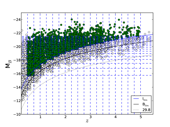
Figure 1: Plot of the B-band absolute magnitudes of the FDF galaxy survey in the redshift range $0.45\leq z\leq 5$. The green filled circles represent the FDF flux-limited I-band selected dataset that would be included in a volume-limited subsample given by the FDF redshift bins and the I-band absolute magnitude cuts of Ir12a, represented here as horizontal dashed blue lines.

The blue bands of G04, in the range $0.5\leq z\leq 5$, were combined in two sets, the blue optical bands $g^{\prime}$ and $B$ and the blue UV bands 1500 Å, 2800 Å and $u^{\prime}$. The red-band dataset of G06, in the range $0.45\leq z\leq 3.75$, was also combined in a single set.

The next step consisted in obtaining observational differential number counts $[\mathrm{d}N/\mathrm{d}z]_{{\textstyle{\scriptscriptstyle\rm obs}}}$ by means of the following expression discussed in detail in Ir12a,

$$\left[\frac{\mathrm{d}N}{\mathrm{d}z}\right]_{{\textstyle{\scriptscriptstyle\rm obs}}}=\frac{V_{\scriptscriptstyle\rm C}}{V_{\scriptscriptstyle\rm Pr}}\frac{\psi}{n}\frac{\mathrm{d}N}{\mathrm{d}z},$$ (14)

where $V_{\scriptscriptstyle\rm C}$ and $V_{\scriptscriptstyle\rm Pr}$ are, respectively, the comoving and proper volumes, $\mathrm{d}N/\mathrm{d}z$ is the theoretical differential number counts and $n$ is the number density of radiating sources in proper volume. All theoretical quantities, that is, $V_{\scriptscriptstyle\rm C}$, $V_{\scriptscriptstyle\rm Pr}$, $n$, $\mathrm{d}N/\mathrm{d}z$, were independently computed in the FLRW spacetime with $\Omega_{m_{\scriptscriptstyle 0}}=0.3$, $\Omega_{\Lambda_{\scriptscriptstyle 0}}=0.7$, $H_{0}=70\;\mbox{km}\;{\mbox{s}}^{-1}\;{\mbox{Mpc}}^{-1}$ and included in the equation above, together with the results of $\psi$ previously obtained, to solve this expression.

Eq. (14) performs essentially a removal of the cosmological model assumed by the observers when they calculated the LF. The aim of this equation is to recover the observed differential number count $[\mathrm{d}N/\mathrm{d}z]_{{\textstyle{\scriptscriptstyle\rm obs}}}$ used by those who built the LF, since to do so they had to assume a cosmology. But, this cosmology extraction does not remove the data corrections, because these were made when the LF was fitted to the data. Therefore, the final $[\mathrm{d}N/\mathrm{d}z]_{{\textstyle{\scriptscriptstyle\rm obs}}}$ data are not really the raw, observed, data, but the fitted raw data. The selection function $\psi$ is the observational part coming directly from the LF, or more specifically, from its integration over absolute magnitudes. $V_{\scriptscriptstyle\rm C}$ and $V_{\scriptscriptstyle\rm Pr}$ are just volume transformations since it is nowadays standard practice to calculate the LF using comoving volume, which has to be removed if we want to obtain number densities using different volume definitions. The theoretical differential number count $\mathrm{d}N/\mathrm{d}z$ and theoretical density $n$ account for the assumed cosmology when the LF was built, but since $n$ is defined in terms of the proper volume, this fact also has to be considered in the extraction of the assumed cosmological model as made by Eq. (14). This cosmology extraction procedure is explained in detail in Ir12a.

The additional necessary steps included computing the cosmological distances $d_{i}$ in the FLRW model with the same cosmological parameters above, integrating $[\mathrm{d}N/\mathrm{d}z]_{{\textstyle{\scriptscriptstyle\rm obs}}}$ to obtain $[N(z)]_{{\textstyle{\scriptscriptstyle\rm obs}}}$ and changing $[\mathrm{d}N/\mathrm{d}z]_{{\textstyle{\scriptscriptstyle\rm obs}}}$ into $[\mathrm{d}N/\mathrm{d}(d_{i})]_{{\textstyle{\scriptscriptstyle\rm obs}}}$. All these results finally allowed the calculation of both $[\gamma_{i}]_{{\textstyle{\scriptscriptstyle\rm obs}}}$ and $[\gamma_{i}^{\ast}]_{{\textstyle{\scriptscriptstyle\rm obs}}}$ according to Eqs. (4) and (7) in the three observational sets above.

It is necessary to point out that although this methodology is capable of extracting from the LF the cosmological model implicitly assumed in its calculation so that the final observational number counts becomes model independent, the standard cosmology enters back into our problem because both $\gamma_{i}$ and $\gamma_{i}^{\ast}$ are function of the cosmological distances $d_{i}$, which themselves require a cosmological model for their evaluation.

As final remarks, we must emphasize again that this work is not about inhomogeneity in the comoving number density, but inhomogeneity defined along the observer’s past light cone. Thus, one can assume a spatial uniform distribution stemming from the standard cosmological model, which is at the heart of the $1/V_{\mathrm{max}}$ LF estimator used in the computation of the LF, obtaining a meaningful $\phi^{*}(z)$, and a relativistic distribution along the past light cone which is not uniform as a result of both expansion effects and the luminosity and/or number density evolution with the redshift in the LF. Such a difference in the manifold foliation where our densities are defined is essential in order to understand our approach. Therefore, relativistic corrections cannot be ignored in any part of our analysis and results, nor can galaxy evolution, especially at large redshifts as is our case here. Our relativistic number densities are a convolution between the geometrical effect of expansion and source evolution, both in the luminosity and number density evolution probed by the LF. Our aim is to find out if this convolution produces observed fractality along the past light cone.

4 Fractal analysis of the FDF survey

The steps described in the previous section provided data on $[\gamma_{i}]_{{\textstyle{\scriptscriptstyle\rm obs}}}$ and $[\gamma_{i}^{\ast}]_{{\textstyle{\scriptscriptstyle\rm obs}}}$ in the three combined observational bands, blue optical, blue UV and red. Once in possession of these results, as well as the ones for $d_{i}\,(z)$ in a FLRW cosmology, we were able to carry out a fractal analysis of the FDF galaxy distribution data by testing their fractal compatibility according to the expressions described in Sect. 2.

4.1 Direct calculation of the fractal dimension

The simplest test is to calculate the fractal dimension by means of Eq. (11). Figure 2 shows graphs of $D$ versus the redshift, where the fractal dimension is estimated by the ratio $D=3[\gamma_{i}]_{{\textstyle{\scriptscriptstyle\rm obs}}}\,/\,[\gamma_{i}^{\ast}]_{{\textstyle{\scriptscriptstyle\rm obs}}}$. The error bars, obtained by standard quadratic propagation, are big. Even so, some conclusions can be drawn from the plots.

Firstly, as predicted by Rangel Lemos and Ribeiro (2008), the fractal dimension decreases as the redshift increases which suggests the absence of an unique fractal dimension at the sample’s redshift intervals. In other words, an unique single fractal system does not seem to be a good approximation to describe the FDF galaxy distribution, since, if that were the case, according to Eq. (11) the graphs in Fig. 2 would have to show an approximate horizontal line indicating a constant fractal dimension. However, due to the big uncertainties such a situation cannot yet be entirely ruled out, although an unique single fractal description seems unlikely.

Secondly, the homogeneous case $D=3$ occurs only very marginally, at the top of very few error bars. Except for a single plot, the red galaxies calculated using $d_{\scriptscriptstyle G}$, all others graphs suggest $D\lesssim 2$ in most of the studied redshift interval. There are very few instances where the top of some error bars show $D>3$, but a fractal system embedded in a three-dimensional topological space cannot have its fractal dimension bigger than the topological dimension and, hence, such values ought to be dismissed. Similarly, the bottom of some error bars reach $D<0$, but as we have discussed above such results are not valid because the number counts is an integral quantity and its exponent in Eq. (8) is either positive or zero and, therefore, these results ought to be dismissed as well. Thus, considering the error bars the fractal dimension is bounded to its maximum allowed range, $0\leq D\leq 3$, but the plots indicate an apparent asymptotic tendency towards $D=0$.

4.2 Calculation of $D$ by power-law fitting

Eqs. (9) and (10) show that both densities should follow a power-law pattern if the galaxy distribution can really be described as a fractal system. Then, performing linear fits in the logarithmic plots of $[\gamma_{i}]_{{\textstyle{\scriptscriptstyle\rm obs}}}$ and $[\gamma_{i}^{\ast}]_{{\textstyle{\scriptscriptstyle\rm obs}}}$ against $d_{i}$ will provide values for $D$. The simplest approach for a fractal description of the galaxy distribution after we dismiss the single fractal approximation is a system with two scaling ranges in the fractal dimension, that is, two consecutive single fractal systems with different fractal dimensions at successive distance ranges.

Next we show the results of a two-straight-lines fit to the data.

4.2.1 Differential density $[\gamma_{i}]_{{\textstyle{\scriptscriptstyle\rm obs}}}$

Fig. 3 shows the plots of all differential densities defined in the three cosmological distances used here against their respective distances. Clearly it is possible to fit two straight lines to the data, whose slopes at different redshift intervals provide values for $D$ by means of Eq. (9). For best fit results, the redshift range can be divided in two intervals, the first being $0.45\leq z\lesssim 1.3-1.9$ and the second one in the range $1.3-1.9\lesssim z\leq 5.0$. Let us call the former as region I and the latter as region II.

The values of D calculated in region I by means of $[\gamma_{\scriptscriptstyle G}]_{{\textstyle{\scriptscriptstyle\rm obs}}}$, $[\gamma_{\scriptscriptstyle L}]_{{\textstyle{\scriptscriptstyle\rm obs}}}$ and $[\gamma_{\scriptscriptstyle z}]_{{\textstyle{\scriptscriptstyle\rm obs}}}$ basically agree with one another in their respective redshift intervals and within the error margins. However, all fractal dimension values obtained in region II are negative and mostly outside the bounds established by the direct method discussed in Sect. 4.1 above, whereas the results in region I are within those bounds. Negative fractal dimensions ought to be dismissed since they are not defined in the context discussed here (see the discussion after Eq. (8) above) and, therefore, only the valid results are summarized in Tables 1 and 2.

The spurious values of the fractal dimension in region II comes from the fact that, by definition, the differential densities measure the rate of growth in number counts, as $\gamma_{i}\propto\mathrm{d}N/\mathrm{d}z$ (see Eq. 4). Inasmuch as $\mathrm{d}N/\mathrm{d}z$ increases, reaches a maximum and then decreases, this behavior substantially enhances the decline in $\gamma$ when $\mathrm{d}N/\mathrm{d}z$ is evaluated at redshift values beyond its maximum. In addition, by measuring a rate of growth in number counts, $\gamma$ is much more sensitive to local fluctuations and noisy data. Thus, the steep decline detected in the slopes of the fitted lines in region II of the $[\gamma_{i}]_{{\textstyle{\scriptscriptstyle\rm obs}}}\times d_{i}$ plots are a consequence of these distortion effects at the redshift limits of the sample, resulting then in spurious negative values for $D$.

The reasoning above being true, we should then expect the absence of such bogus negative fractal dimension values when they are calculated with the integral densities in similar $[\gamma_{i}^{\ast}]_{{\textstyle{\scriptscriptstyle\rm obs}}}\times d_{i}$ plots, because $\gamma_{i}^{\ast}\propto N$ (see Eq. 7). As the cumulative number counts $N$ only grows or stays constant, describing therefore the change in number counts for the entire observational volume, this property also renders $\gamma_{i}^{\ast}$ less sensitive to tail fluctuations. Hence, $\gamma_{i}^{\ast}$ should not present an enhanced decline distortion at the tail of the distribution and the values for $D$ obtained with $\gamma_{i}^{\ast}$ should also not assume phony negative values. As we shall see below this is what really happens.

4.2.2 Integral density $[\gamma_{i}^{\ast}]_{{\textstyle{\scriptscriptstyle\rm obs}}}$

The same division in two regions was assumed in order to fit straight lines to the data plots of the integral density versus their respective cosmological distances. Fig. 4 shows the $[\gamma_{i}^{\ast}]_{{\textstyle{\scriptscriptstyle\rm obs}}}\times d_{i}$ plots where the fractal dimension was calculated by estimating the power-law exponent as given in Eq. (10). The results are summarized in Tables 3 and 4.

The calculated figures show an absence of negative values for the fractal dimension in region II, even considering the error margins, as predicted above. Besides, all results are well within the bounds established in Sect. 4.1. Thirdly, although the values of $D$ obtained from the $[\gamma_{i}^{\ast}]_{{\textstyle{\scriptscriptstyle\rm obs}}}\times d_{i}$ plots in region I are somewhat higher than those obtained in the same region by the $[\gamma_{i}]_{{\textstyle{\scriptscriptstyle\rm obs}}}\times d_{i}$ plots, they are consistent, or very closely consistent, with each other considering the calculated uncertainties. This reinforces the view that the results for $D$ obtained in region II from the $[\gamma_{i}]_{{\textstyle{\scriptscriptstyle\rm obs}}}\times d_{i}$ plots are indeed spurious, especially nearby the limits of the sample.

4.3 Discussion

In order to better examine the results above, let us calculate averages for the fractal dimensions in regions I and II for all galaxy types but, specifying if they were obtained by the differential or integral number densities. These averages are as follows,

$${\langle D\rangle}_{I}^{\gamma}=0.8^{\scriptscriptstyle+0.7}_{\scriptscriptstyle-0.7}\>,\;\;{\langle D\rangle}_{I}^{\gamma^{\ast}}=1.4^{\scriptscriptstyle+0.7}_{\scriptscriptstyle-0.6}\>,\;\;{\langle D\rangle}_{II}^{\gamma^{\ast}}=0.5^{\scriptscriptstyle+1.2}_{\scriptscriptstyle-0.4}\>.$$ (15)

We have dismissed the result for ${\langle D\rangle}_{II}^{\gamma}$ due to its spurious nature, as discussed above. We note that due to the data diversity and limitation, that is, different types of galaxies and an analysis of a single survey which probed a very limited part of the sky, these results should be considered only as general estimates, but they allow us to reach some conclusions.

Firstly, it is clear that we can consider the galaxy distribution as being described by a bi-fractal system, at least as far as the FDF data is concerned. Secondly, despite being different, the values of ${\langle D\rangle}_{I}^{\gamma}$ and ${\langle D\rangle}_{I}^{\gamma^{\ast}}$ agree with one another within the error margins. This allows us to reach a third conclusion, which is that up to $z\sim 1.5$ the fractal dimension is probably in the range $D=1-2$, whereas for $1.5\lesssim z\lesssim 5.0$ we probably have $D=0-1$. It is also clear that the integral density provides a much better tool for estimating the fractal dimension, since it does not produce bogus negative values for $D$ at higher redshifts. Finally, the results show that a fractal analysis of the large-scale galaxy distribution could potentially bring insights in its evolution as $D$ could provide a parameter for void evolution. This is so because a decreasing fractal dimension at increasing redshift ranges indicates that in the past galaxies and galaxy clusters were much more sparsely distributed than at recent epochs, possibly meaning a more dominant role for voids in the large-scale galactic structure at those earlier times.

5 Conclusions

In this paper we have performed a fractal analysis of the galaxy distribution of the FORS Deep Field (FDF) galaxy redshift survey in the range $0.45\leq z\leq 5.0$ under the assumption that this distribution forms a fractal system. The cosmological distances $d_{i}$ and their respective observed differential and integral number densities $[\gamma_{i}]_{{\textstyle{\scriptscriptstyle\rm obs}}}$ and $[\gamma_{i}^{\ast}]_{{\textstyle{\scriptscriptstyle\rm obs}}}$ were used to calculate the fractal dimension $D$ of the fractal galactic system by two methods: the direct calculation, through the expression $D=3[\gamma_{i}]_{{\textstyle{\scriptscriptstyle\rm obs}}}/[\gamma_{i}^{\ast}]_{{\textstyle{\scriptscriptstyle\rm obs}}}$, and by linear fitting, to extract $D$ from the exponents of the power-laws formed by the plots $[\gamma_{i}]_{{\textstyle{\scriptscriptstyle\rm obs}}}\times d_{i}$ and $[\gamma_{i}^{\ast}]_{{\textstyle{\scriptscriptstyle\rm obs}}}\times d_{i}$. The index $i$ stands for ($i={\scriptstyle G}$, ${\scriptstyle L}$, ${\scriptstyle Z}$) according to the three cosmological distances used in this paper, the galaxy area distance $d_{\scriptscriptstyle G}$, the luminosity distance $d_{\scriptscriptstyle L}$ and the redshift distance $d_{z}$. We have used the observed number densities $[\gamma_{i}]_{{\textstyle{\scriptscriptstyle\rm obs}}}$ and $[\gamma_{i}^{\ast}]_{{\textstyle{\scriptscriptstyle\rm obs}}}$ previously calculated by Iribarrem et al. (2012a) in the standard FLRW cosmological model with $\Omega_{m_{\scriptscriptstyle 0}}=0.3$, $\Omega_{\Lambda_{\scriptscriptstyle 0}}=0.7$ and $H_{0}=70\;\mbox{km}\;{\mbox{s}}^{-1}\;{\mbox{Mpc}}^{-1}$ using the luminosity function parameters of the FDF survey as computed by Gabasch et al. (2004, 2006) by means of a Schechter analytical profile. Both $[\gamma_{i}]_{{\textstyle{\scriptscriptstyle\rm obs}}}$ and $[\gamma_{i}^{\ast}]_{{\textstyle{\scriptscriptstyle\rm obs}}}$ were computed in the three sets of combined galaxy types adopted by Ir12a, namely blue optical, blue UV and red galaxies, and a cut in absolute magnitudes was used to select the galaxies that entered in the computation of both quantities.

Although the adopted galaxy sample probed a limited part of the sky, it has the advantage of being deep enough for the inhomogeneous irregularities of the galaxy distribution to be detected along the past light cone even in the spatially homogeneous standard FLRW cosmological model adopted here. These inhomogeneities are better detected by $[\gamma^{\ast}]_{{\textstyle{\scriptscriptstyle\rm obs}}}$, since $[\gamma]_{{\textstyle{\scriptscriptstyle\rm obs}}}$ is subject to an important distortion leading to a steep decline in its computed values at high redshift values, an effect which renders the results obtained with $[\gamma]_{{\textstyle{\scriptscriptstyle\rm obs}}}$ more error prone.

The direct calculation of $D$ produced results within the allowed boundaries of the fractal dimension, $0\leq D\leq 3$, when error bars are considered, but suggested an asymptotic tendency towards $D=0$ as $z$ increases. This direct method also showed (i) an evolution of the fractal dimension, since $D$ decreases as $z$ increases, (ii) that the homogeneous case $D=3$ is only marginally obtained even at low redshift values and (iii) that an unique single fractal system encompassing the whole redshift range of the FDF sample is not a good approximation to describe the FDF galaxy distribution.

Calculating the fractal dimension by means of the exponent of the power-laws formed by the $[\gamma_{i}]_{{\textstyle{\scriptscriptstyle\rm obs}}}\times d_{i}$ and $[\gamma_{i}^{\ast}]_{{\textstyle{\scriptscriptstyle\rm obs}}}\times d_{i}$ plots showed that the best fits were obtained by considering the galaxy distribution as being bi-fractal, that is, characterized by two scaling ranges in the fractal dimension. In other words, by bi-fractal we mean two fractal regimes, or two single fractal systems, at different and successive ranges. The first set of values for the fractal dimension were calculated in the range $0.45\leq z\lesssim 1.3-1.9$, named as region I, whereas the second set of values for $D$, named region II, was defined by the redshift range $1.3-1.9\lesssim z\leq 5.0$. Average results indicated that the fractal dimension varies from $D=2$ to $D=1$ in region I and from $D=1$ to $D=0$ in region II. Such evolution of the fractal dimension could provide insights on how the large-scale galactic structure evolves, since these results suggest that in the past individual galaxies and galactic clusters were much more sparsely distributed than at later epochs and, therefore, the Universe was then possibly dominated by voids.

Finally, it is worth mentioning that Iribarrem et al. (2013) fitted the luminosity function in a Lemaître-Tolman-Bondi (LTB) spatially inhomogeneous cosmological model using over 10,000 sources of the Herschel/PACS evolutionary probe (PEP) survey in the observer’s far-infrared passbands of 100 $\mu$m and 160 $\mu$m. Then Iribarrem et al. (2014) used those results to obtain power-law fits for both $[\gamma_{\scriptscriptstyle L}]_{{\textstyle{\scriptscriptstyle\rm obs}}}$ and $[\gamma_{\scriptscriptstyle L}^{\ast}]_{{\textstyle{\scriptscriptstyle\rm obs}}}$ in the high redshift range $1.5\lesssim z\lesssim 3.2$ (see their Fig. 6). Although Iribarrem et al. (2014) focused on other issues, one can infer from their results for $[\gamma_{\scriptscriptstyle L}^{\ast}]_{{\textstyle{\scriptscriptstyle\rm obs}}}\times d_{\scriptscriptstyle L}$ in both 100 $\mu$m and 160 $\mu$m passbands that they produced $\langle D\rangle=0.6\pm 0.1$, that is, an average value comparable to the high redshift fractal dimension found in the red region of the FDF survey studied in this paper using the FLRW cosmology (see table 3 below).

We thank A. R. Lopes for kindly providing her results obtained with the FDF data and for useful discussions. We also thank four referees for their comments and useful suggestions which improved the paper. G. C.-S. and A. I. are grateful to the Brazilian agency CAPES for financial support.

Table 1: Fractal dimensions calculated using $[\gamma_{\scriptscriptstyle L}]_{{\textstyle{\scriptscriptstyle\rm obs}}}$ and $[\gamma_{\scriptscriptstyle z}]_{{\textstyle{\scriptscriptstyle\rm obs}}}$

galaxies	$z$	$[\gamma_{\scriptscriptstyle L}]_{{\textstyle{\scriptscriptstyle\rm obs}}}\times d_{\scriptscriptstyle L}$	$[\gamma_{\scriptscriptstyle z}]_{{\textstyle{\scriptscriptstyle\rm obs}}}\times d_{z}$
blue optical	$0.5-1.2$	$D=0.6\pm 0.3$	$D=0.7\pm 0.4$
	$1.3-5.0$	$-$	$-$
blue UV	$0.5-1.2$	$D=0.4\pm 0.3$	$D=0.6\pm 0.3$
	$1.3-5.0$	$-$	$-$
red	$0.45-1.15$	$D=0.8\pm 0.3$	$D=1.0\pm 0.3$
	$1.25-3.75$	$-$	$-$

Table 2: Fractal dimensions calculated using $[\gamma_{\scriptscriptstyle G}]_{{\textstyle{\scriptscriptstyle\rm obs}}}$

galaxies	$z$	$[\gamma_{\scriptscriptstyle G}]_{{\textstyle{\scriptscriptstyle\rm obs}}}\times d_{\scriptscriptstyle G}$
blue optical	$0.5-1.8$	$D=1.0\pm 0.3$
	$1.9-5.0$	$-$
blue UV	$0.5-1.8$	$D=0.8\pm 0.3$
	$1.9-5.0$	$-$
red	$0.45-1.75$	$D=1.3\pm 0.3$
	$1.85-3.75$	$-$

Table 3: Fractal dimensions calculated using $[\gamma_{\scriptscriptstyle L}^{\ast}]_{{\textstyle{\scriptscriptstyle\rm obs}}}$ and $[\gamma_{\scriptscriptstyle z}^{\ast}]_{{\textstyle{\scriptscriptstyle\rm obs}}}$

galaxies	$z$	$[\gamma_{\scriptscriptstyle L}^{\ast}]_{{\textstyle{\scriptscriptstyle\rm obs}}}\times d_{\scriptscriptstyle L}$	$[\gamma_{\scriptscriptstyle z}^{\ast}]_{{\textstyle{\scriptscriptstyle\rm obs}}}\times d_{z}$
blue optical	$0.5-1.2$	$D=1.1\pm 0.3$	$D=1.6\pm 0.4$
	$1.3-5.0$	$D=0.3\pm 0.1$	$D=0.4\pm 0.1$
blue UV	$0.5-1.2$	$D=1.1\pm 0.3$	$D=1.3\pm 0.3$
	$1.3-5.0$	$D=0.3\pm 0.1$	$D=0.3\pm 0.1$
red	$0.45-1.15$	$D=1.2\pm 0.3$	$D=1.5\pm 0.4$
	$1.25-3.75$	$D=0.5\pm 0.2$	$D=0.6\pm 0.2$

Table 4: Fractal dimensions calculated using $[\gamma_{\scriptscriptstyle G}^{\ast}]_{{\textstyle{\scriptscriptstyle\rm obs}}}$

galaxies	$z$	$[\gamma_{\scriptscriptstyle G}^{\ast}]_{{\textstyle{\scriptscriptstyle\rm obs}}}\times d_{\scriptscriptstyle G}$
blue optical	$0.5-1.8$	$D=1.6\pm 0.3$
	$1.9-5.0$	$D=0.7\pm 0.5$
blue UV	$0.5-1.8$	$D=1.5\pm 0.2$
	$1.9-5.0$	$D=0.5\pm 0.4$
red	$0.45-1.75$	$D=1.8\pm 0.3$
	$1.85-3.75$	$D=1.0\pm 0.7$

$\begin{array}[]{ccc}\includegraphics[width=150.79968pt]{rategammaGOpt}&\includegraphics[width=150.79968pt]{rategammaGUV}&\includegraphics[width=150.79968pt]{rategammaGRed}\\ \includegraphics[width=150.79968pt]{RateGamaLblueOpt}&\includegraphics[width=150.79968pt]{RateGamaLblueUV}&\includegraphics[width=150.79968pt]{RateGamaLred}\\ \includegraphics[width=150.79968pt]{RateGamaZblueOpt}&\includegraphics[width=150.79968pt]{RateGamaZblueUV}&\includegraphics[width=150.79968pt]{RateGamaZred}\end{array}$

Figure 2: Fractal dimensions calculated with $[\gamma_{i}]_{{\textstyle{\scriptscriptstyle\rm obs}}}$ and $[\gamma_{i}^{\ast}]_{{\textstyle{\scriptscriptstyle\rm obs}}}$ using Eq. (11).

$\begin{array}[]{ccc}\includegraphics[width=150.79968pt]{gammaGOPT}&\includegraphics[width=150.79968pt]{gammaGUV}&\includegraphics[width=150.79968pt]{gammaGRED}\\ \includegraphics[width=150.79968pt]{gammaLOpt}&\includegraphics[width=150.79968pt]{gammaLUV}&\includegraphics[width=150.79968pt]{gammaLRed}\\ \includegraphics[width=150.79968pt]{gammaZOpt}&\includegraphics[width=150.79968pt]{gammaZUV}&\includegraphics[width=150.79968pt]{gammaZRed}\end{array}$

Figure 3: Graphs of $[\gamma_{i}]_{{\textstyle{\scriptscriptstyle\rm obs}}}\times d_{i}$. $D$ is obtained by a double linear fitting according to Eq. (9).

$\begin{array}[]{ccc}\includegraphics*[width=150.79968pt]{ngopt}&\includegraphics*[width=150.79968pt]{nguv}&\includegraphics*[width=150.79968pt]{ngred}\\ \includegraphics*[width=150.79968pt]{nLOpt}&\includegraphics*[width=150.79968pt]{nLUV}&\includegraphics*[width=150.79968pt]{nLRed}\\ \includegraphics*[width=150.79968pt]{nZOpt}&\includegraphics*[width=150.79968pt]{nZUV}&\includegraphics*[width=150.79968pt]{nZRed}\end{array}$

Figure 4: Graphs of $[\gamma_{i}^{\ast}]_{{\textstyle{\scriptscriptstyle\rm obs}}}\times d_{i}$. $D$ is obtained by a double linear fitting according to Eq. (10).

References

- [1] Abdalla, E., Afshordi, N., Khodjasteh, K., and Mohayaee, R. 1999, A&A, 345, 22
- [2] Abdalla, E., and Chirenti, C. B. M. H. 2004, Physica A, 337, 117
- [3] Abdalla, E., Mohayaee, R., and Ribeiro, M.B. 2001, Fractals 9, 451; arXiv:astro-ph/9910003
- [4] Albani, V. V. L., Iribarrem, A. S., Ribeiro, M. B., and Stoeger, W. R. 2007, ApJ, 657, 760; arXiv:astro-ph/0611032 (A07)
- [5] Amoroso Costa, M. 1929, Annals of Brazilian Acad. Sci. 1, 51, (in Portuguese)
- [6] Baryshev, I., and Teerikorpi, P. 2002, The Discovery of Cosmic Fractals (World Scientific, Singapore)
- [7] Carpenter, E. F. 1938, ApJ, 88, 344
- [8] Charlier, C. V. L. 1908, Ark. Mat. Astr. Fys., 4, 1
- [9] Charlier, C. V. L. 1922, Ark. Mat. Astr. Fys., 16, 1
- [10] de Vaucouleurs, G. 1960, ApJ, 131, 585
- [11] de Vaucouleurs, G. 1970, Science, 167, 1203
- [12] Einstein, A. 1922, Ann. Phys., 69, 436
- [13] Ellis, G. F. R. 1971, in General Relativity and Cosmology, ed. R. K. Sachs, Proc. Int. School Phys. Enrico Fermi (Academic Press, New York); reprinted in Gen. Rel. Grav., 41 (2009) 581
- [14] Ellis, G. F. R. 2007, Gen. Rel. Grav., 39, 1047
- [15] Etherington, I. M. H. 1933, Phil. Mag., 15, 761; reprinted in Gen. Rel. Grav., 39 (2007) 1055
- [16] Gabasch, A., Bender, R., Seitz, S., Hopp, U. et al. 2004, A&A, 421, 41 (G04)
- [17] Gabasch, A., Hopp, U., Feulner, G., Bender, R. et al. 2006, A&A, 448, 101 (G06)
- [18] Gabrielli, A., Sylos Labini, F., Joyce, M., and Pietronero, L. 2005, Statistical Physics for Cosmic Structures (Springer, Berlin)
- [19] Grujić, P. V. 2011, Serbian Astron. J., Nr. 182, 1
- [20] Haggerty, M. J., and Wertz, J. R. 1972, MNRAS, 155, 495
- [21] Iribarrem, A. S., Lopes, A. R., Ribeiro, M. B., and Stoeger, W. R. 2012a, A&A, 539, A112; arXiv:1201.5571 (Ir12a)
- [22] Iribarrem, A. S., Ribeiro, M. B., and Stoeger, W. R. 2012b, in Proc. 12th Marcel Grossmann Meeting, ed. T. Damour, R. T. Jantzen and R. Ruffini, (World Scientific, Singapore), 2216; arXiv:1207.2542
- [23] Iribarrem, A., Andreani, P., Gruppioni, C., February, S., Ribeiro, M. B. et al. 2013, A&A, 558, A15; arXiv:1308.2199
- [24] Iribarrem, A., Andreani, P., February, S., Gruppioni, C., Lopes, A. R., Ribeiro, M. B., and Stoeger, W. R. 2014, A&A, 563, A20; arXiv:1401.6572
- [25] Lin, H., Yee, H. K. C., Carlberg, R. G., Morris, S. L. et al. 1999, ApJ, 518, 533
- [26] Mandelbrot, B. B. 1983, The Fractal Geometry of Nature (Freeman, New York)
- [27] Mureika, J. R. 2007, JCAP, 05:021
- [28] Mureika, J. R. and Dyer, C.C. 2004, Gen. Rel. Grav., 36, 151
- [29] Pietronero, L. 1987, Physica A, 144, 257
- [30] Rangel Lemos, L. J., and Ribeiro, M. B. 2008, A&A, 488, 55; arXiv:0805.3336
- [31] Ribeiro, M. B. 1992a, ApJ, 388, 1; arXiv:0807.0866
- [32] Ribeiro, M. B. 1992b, ApJ, 395, 29; arXiv:0807.0869
- [33] Ribeiro, M. B. 1993, ApJ, 415, 469; arXiv:0807.1021
- [34] Ribeiro, M. B. 1994, Deterministic Chaos in General Relativity, eds. D. W. Hobill, A. Burd, and A. Coley (Plenum, New York), p. 269; arXiv:0910.4877
- [35] Ribeiro, M. B. 1995, ApJ, 441, 477; arXiv:astro-ph/9910145
- [36] Ribeiro, M. B. 2001a, Fractals, 9, 237; arXiv:gr-qc/9909093
- [37] Ribeiro, M. B. 2001b, Gen. Rel. Grav., 33, 1699; arXiv:astro-ph/0104181
- [38] Ribeiro, M. B. 2005, A&A, 429, 65; arXiv:astro-ph/0408316
- [39] Ribeiro, M. B., and Miguelote, A. Y. 1998, Braz. J. Phys., 28, 132; arXiv:astro-ph/9803218
- [40] Ribeiro, M. B., and Stoeger, W. R. 2003, ApJ, 592, 1; arXiv:astro-ph/0304094
- [41] Selety, F. 1922, Ann. Phys., 68, 281
- [42] Sylos Labini, F. 2011, Class. Quantum Grav., 28, 164003
- [43] Sylos Labini, F., Montuori, M., and Pietronero, L. 1998, Phys. Rep., 293, 61
- [44] Wertz, J. R. 1970, Newtonian Hierarchical Cosmology, Ph.D. Thesis, University of Texas at Austin
- [45] Wertz, J. R. 1971, ApJ, 164, 227