SAME but Different: Fast and High-Quality Gibbs Parameter Estimation

Abstract

Gibbs sampling is a workhorse for Bayesian inference but has several limitations when used for parameter estimation, and is often much slower than non-sampling inference methods. SAME (State Augmentation for Marginal Estimation) [14, 8] is an approach to MAP parameter estimation which gives improved parameter estimates over direct Gibbs sampling. SAME can be viewed as cooling the posterior parameter distribution and allows annealed search for the MAP parameters, often yielding very high quality (lower loss) estimates. But it does so at the expense of additional samples per iteration and generally slower performance. On the other hand, SAME dramatically increases the parallelism in the sampling schedule, and is an excellent match for modern (SIMD) hardware. In this paper we explore the application of SAME to graphical model inference on modern hardware. We show that combining SAME with factored sample representation (or approximation) gives throughput competitive with the fastest symbolic methods, but with potentially better quality. We describe experiments on Latent Dirichlet Allocation, achieving speeds similar to the fastest reported methods (online Variational Bayes) and lower cross-validated loss than other LDA implementations. The method is simple to implement and should be applicable to many other models.

1 Introduction

Many machine learning problems can be formulated as inference on a joint distribution $P(X,Z,\Theta)$ where $X$ represents observed data, $\Theta$ a set of parameters, and $Z$ represents latent variables. Both $\Theta$ and $Z$ are latent in general, but it is useful to distinguish between them - $\Theta$ encodes which of a class of models represents the current situation, while $Z$ represent local labels or missing data. One generally wants to optimize over $\Theta$ while marginalizing over $Z$. And the output of the algorithm is a value or distribution over $\Theta$ while the $Z$ are often ignored.

Gibbs sampling is a very general approach to posterior estimation for $P(X,Z,\Theta)$, but it provides samples only rather than MAP estimates. But therein lies a problem: sampling is a sensible approach to marginal estimation, but can be a very inefficient approach to optimization. This is particularly true when the dimension of $\Theta$ is large compared to $X$ (which is true e.g. in Latent Dirichlet Allocation and probabilistic recommendation algorithms). Such models have been observed to require many samples (thousands to hundreds of thousands) to provide good parameter estimates. Hybrid approaches such as Monte-Carlo EM have been developed to address this issue - a Monte-Carlo method such as Gibbs sampling is used to estimate the expected values in the E-step while an optimization method is applied to the parameters in the M-step. But this requires a separate optimization strategy (usually gradient-based), a way to compute the dependence on the parameters symbolically, and analysis of the accuracy of the E-step estimates.

SAME (State Augmentation for Marginal Estimation) [14, 8] is a simple approach to MAP parameter estimation that remains within the Gibbs framework. SAME replicates the latent state $Z$ with additional states. This has the effect of “cooling” the marginal distribution on $\Theta$, which sharpens its peaks and causes $\Theta$ samples to approach local optima. The conditional distribution $P(Z|X,\Theta)$ remains the same, so we are still marginalizing over a full distribution on $Z$. By making the temperature a controllable parameter, the parameter estimates can be annealed to reach better local optima. In both [14, 8] and the present paper we find that this approach gives better estimates than competing approaches. The novelty of the present paper is showing that SAME estimation can be very fast, and competitive with the fastest symbolic meethods. Thus it holds the potential to be the method of choice for many inference problems.

Specifically, we define a new joint distribution

$$P^{\prime}(X,\Theta,Z^{(1)},\ldots,Z^{(m)})=\prod_{j=1}^{m}P(X,\Theta,Z^{(j)})$$ (1)

which models $m$ copies of the original system with tied parameters $\Theta$ and independent latent variable blocks $Z^{(1)},\ldots,Z^{(m)}$. The marginalized conditional $P^{\prime}(\Theta|X)=P^{\prime}(X,\Theta)/P(X)$. And

$$P^{\prime}(X,\Theta)=\int_{Z^{(1)}}\cdots\int_{Z^{(m)}}\prod_{j=1}^{m}P(X,\Theta,Z^{(j)})~{}dZ^{(1)}\cdots dZ^{(m)}=\prod_{j=1}^{m}P(X,\Theta)=P^{m}(X,\Theta)$$ (2)

where $P(X,\Theta)=\int_{Z}P(X,\Theta,Z)~{}dZ$. So $P^{\prime}(\Theta|X)=P^{m}(X,\Theta)/P(X)$ which is up to a constant factor equal to $P^{m}(\Theta|X)$, a power of the original marginal parameter distribution. Thus it has the same optima, including the global optimum, but its peaks are considerably sharpened. In what follows we will often demote $X$ to a subscript since it fixed, writing $P(\Theta|Z,X)$ as $P_{X}(\Theta|Z)$ etc.

This new distribution can be written as a Gibbs distribution on $\Theta$, as $P^{m}(\Theta,X)=\exp(-mg_{X}(\Theta))=\exp(-g_{X}(\Theta)/(kT))$, from which we see that $m=1/(kT)$ is an inverse temperature parameter ($k$ is Boltzmann’s constant). Increasing $m$ amounts to cooling the distribution.

Gibbs sampling from the new distribution is usually straightforward given a sampler for the original. It is perhaps not obvious why sampling from a more complex system could improve performance, but we have added considerable parallelism since we can sample various “copies” of the system concurrently. It will turn out this approach is complementary to using a factored form for the posterior. Together these methods gives us orders-of-magnitude speedup over other samplers for LDA.

The rest of the paper is organized as follows. Section 2 summarizes related work on parameter inference for probabilistic models and their limitations. Section 3 introduces the SAME sampler. We discuss in Section 4 a factored approximation that considerably accelerates sampling. A hardware-optimized implementation of the algorithm for LDA is described in Section 5. Section 6 presents the experimental results and finally Section 7 concludes the paper.

2 Related Work

2.1 EM and related Algorithms

The Expectation-Maximization (EM) algorithm [7] is a popular method for parameter estimation of graphical models of the form we are interested in. The EM algorithm alternates between updates in the expectation (E) step and maximization (M) step. The E-step marginalizes out the latent variables and computes the expectation of the likelihood as a function of the parameters. The E step computes a $Q$ function $Q(\Theta^{\prime}|\Theta)=E_{Z|\Theta}(\log P_{X}(Z,\Theta^{\prime}))$ to be optimized in the M-step.

For EM to work, one has to compute the expectation of the sufficient statistics of the likelihood function, where the expectation is over $Z|\Theta$. It also requires a method to optimize the $Q$ function. In practice, the iterative update equations can be hard to derive. Moreover, the EM algorithm is a gradient-based method, and therefore is only able to find locally-optimal solutions.

Variational Bayes (VB) [12] is an EM-like algorithm that uses a parametric approximation to the posterior distribution of both parameters and other latent variables, and attempts to optimize the fit (e.g. using KL-divergence) to the observed data. Parameter estimates are usually taken from the means of the parameter approximations (the hyperparameters), unlike EM where point parameter estimates are used. It is common to assume a coordinate-factored form for this approximate posterior. The factored form simplifies inference, but makes strong assumptions about the distribution (effectively eliminating interactions). It makes most sense for parameter estimates, but is a strong constraint to apply to other latent variables. VB has been criticized for lack of quality (higher loss) on certain problems because of this. Nevertheless it works well for many problems (e.g. on LDA). This motivated us to introduce a similar factored approximation in our method described laster.

2.2 Gibbs Sampling

Gibbs samplers [9] work by stepping through individual (or blocks of) latent variables, and in effect perform a simulation of the stochastic system described by the joint distribution. The method is simple to apply on graphical models since each variable is conditioned locally by its Markov blanket. They are easy to define for conjugate distributions and can generalize to non-conjugate graphical models using e.g. slice sampling. Gibbs samplers are often the first method to be derived, and sometimes the only practical learning strategy for complex graphical models.

Gibbs samplers only require that the joint density is strictly positive over the sample space which is known as the Gibbs distribution. However, Gibbs sampling only gives samples from the distribution of $\Theta$, it can be difficult to find ML or MAP values from those samples. Furthermore, it can be very slow, especially for models with high dimensions. Our results suggest this slow convergence is often due to large variance in the parameters in standard samplers.

2.3 Monte Carlo EM

Monte Carlo EM [15] is a hybrid approach that uses MCMC (e.g. Gibbs sampling) to approximate the expected value $E_{Z|\Theta}(\log P_{X}(Z,\Theta^{\prime}))$ with the mean of the log-likelihood of the samples. The method has to optimize $Q(\Theta^{\prime}|\Theta)$ using a numerical method (conjugate gradient etc.). Like standard EM, it can suffer from convergence problems, and may only find a local optimum of likelihood.

2.4 Message-Passing Methods

Belief propagation [16] and Expectation propagation [13] use local (node-wise) updates to infer posterior parameters in graphical models in a manner reminiscent of Gibbs sampling. But they are exact only for a limited class of models. Recently variational message-passing [17] has extended the class of models for which parametric inference is possible to conjugate-exponential family graphical models. However similar to standard VB, the method uses a coordinate-factored approximation to the posterior which effectively eliminates interactions (although they can be added at high computational cost by using a factor graph). It also finds only local optima of the posterior parameters.

3 SAME Parameter Estimation

SAME estimation involves sampling multiple $Z$’s independently and inferring $\Theta$ using the aggregate of $Z$’s.

3.1 Method

We use the notation $Z_{-i}=Z_{1},\ldots,Z_{i-1},Z_{i+1},\ldots,Z_{n}$ and similarly for $\Theta_{-i}$.

Algorithm 1 Standard Gibbs Parameter Estimation

1:initialize parameters $\Theta$ randomly, then in some order:

2:Sample $Z_{i}\sim P_{X}(Z_{i}|Z_{-i},\Theta)$

3:Sample $\Theta_{i}\sim P_{X}(\Theta_{i}|\Theta_{-i},Z)$

Algorithm 2 SAME Parameter Estimation

1:initialize parameters $\Theta$ randomly, and in some order:

2:Sample $Z^{(j)}_{i}\sim P_{X}(Z_{i}^{(j)}|Z^{(j)}_{-i},\Theta)$

3:Sample $\Theta_{i}\sim P_{X}(\Theta_{i}|\Theta_{-i},Z^{(1)},\ldots,Z^{(m)})$

Sampling $Z_{i}^{(j)}$ in the SAME sampler is exactly the same as for the standard sampler. Since the groups $Z^{(j)}$ are independent of each other, we can use the sampling function for the original distribution, conditioned only on the other components of the same group: $Z_{-i}^{(j)}$.

Sampling $\Theta_{i}$ is only slightly more complicated. We want to sample from

$$P_{X}(\Theta_{i}|\Theta_{-i},Z^{(1)},\ldots,Z^{(m)})=P_{X}(\Theta,\overline{Z})/P_{X}(\Theta_{-i},\overline{Z})$$ (3)

where $\overline{Z}=Z^{(1)},\ldots,Z^{(m)}$ and if we ignore the normalizing constants:

$$P_{X}(\Theta,\overline{Z})/P_{X}(\Theta_{-i},\overline{Z})\propto P_{X}(\Theta,\overline{Z})=\prod_{j=1}^{m}P_{X}(\Theta,Z^{(j)})\propto\prod_{j=1}^{m}P_{X}(\Theta_{i}|\Theta_{-i},Z^{(j)})$$ (4)

which is now expressed as a product of conditionals from the original sampler $P_{X}(\Theta_{i}|\Theta_{-i},Z^{(j)})$. Inference in the new model will be tractable if we are able to sample from a product of the distributions $P_{X}(\Theta_{i}|\Theta_{-i},Z^{(j)})$. This will be true for many distributions. e.g. for exponential family distributions in canonical form, the product is still an exponential family member. A product of Dirichlet distributions is Dirichlet etc., and in general this distribution represents the parameter estimate obtained by combining evidence from independent observations. The normalizing constant will usually be implied from the closed-form parameters of this distribution.

Adjusting sample number $m$ at different iterations allows annealing of the estimate.

4 Coordinate-Factored Approximation

Certain distributions (including LDA) have the property that the latent variables $Z_{i}$ are independent given $X$ and $\Theta$. That is $P(Z_{i}|Z_{-i},X,\Theta)=P(Z_{i}|X,\Theta)$. Therefore the $Z_{i}$’s can be sampled (without approximation) in parallel. Furthermore, rather than a single sample from $P(Z_{i}|X,\Theta)$ (e.g. a categorical sample for a discrete $Z_{i}$) we can construct a SAME Gibbs sampler by taking $m$ samples. These samples will now have a multinomial distribution with count $m$ and probability vector $P(Z_{i}|X,\Theta)$. Let $\hat{Z}_{i}(v)$ denote the count for $Z_{i}=v$ among the $m$ samples, and $P(Z_{i}=v|X,\Theta)$ denote the conditional probability that $Z_{i}=v$.

We can introduce still more parallelism by randomizing the order in which we choose which $Z_{i}$ from which to sample. The count $m$ for variable $Z_{i}$ is then replaced by random variable $\hat{m}\sim\text{Poisson}(m)$ and the coordinate-wise distributions of $\hat{Z}_{i}$ become independent Poisson variables:

$$\hat{Z}_{i}(v)\sim\text{Poisson}(mP(Z_{i}=v|X,\Theta))$$ (5)

when the $Z_{i}$ are independent given $X,\Theta$, the counts $\hat{Z}_{i}(v)$ fully capture the results of taking the $m$ (independent) samples. These samples can be generated very fast, and completely in parallel. $m$ is no longer constrained to be an integer, or even to be $>1$. Indeed, each sample no longer corresponds to execution of a block of code, but is simply an increment in the value $m$ of the Poisson random number generator. In LDA, it is almost as fast to generate all $m$ samples for a single word for a large $m$ (up to about 100) as it is to generate one sample. This is a source of considerable speedup in our LDA implementation.

For distributions where the $Z_{i}$ are not independent, i.e. when $P(Z_{i}|Z_{-i},X,\Theta)\neq P(Z_{i}|X,\Theta)$, we can still perform independent sampling as an approximation. This approach is quite similar to the coordinate-factored approximation often used in Variational Bayes. We leave the details to a forthcoming paper.

5 Implementation of SAME Gibbs LDA

Our SAME LDA sampler implementation is described in Algorithm 3. Samples are taken directly from Poisson distributions (line $7$ of the algorithm) as described earlier.

5.1 Latent Dirichlet Allocation

LDA is a generative process for modeling a collection of documents in a corpus. In the LDA model, the words $X=\{x_{d,i}\}$ are observed, the topics $Z=\{z_{d,i}\}$ are latent variables and parameters are $\Theta=(\theta,\phi)$ where $\theta$ is document topic distributions and $\phi$ is word topic distributions. Subscript $d,i$ denotes document $d$ and its $i^{th}$ word. Given $X$ and $\Theta$, $z_{d,i}$ are independent, which also implies that we can sample from $Z$ without any information about $Z$ from previous samples. A similar result holds for the parameters, which can be sampled given only the current counts from the $Z_{i}$. We can therefore alternate parameter and latent variable inference using a pair of samplers: $P_{X}(Z|\theta,\phi)$ and $P_{X}(\theta,\phi|Z)$. Such blocked sampling maximizes parallelism and works very well with modern SIMD hardware.

The sampling of $z_{d,i}$’s uses the Poisson formula derived earlier. The conditional distributions $P_{X}(\theta,\phi|z_{d,i})$ are multiple independent Dirichlet’s. In practice, we collapse out $(\theta,\phi)$, so we in effect sample a new $z_{d,i}^{t}$ given the $z^{t-1}$ from a previous iteration. The update sampler follows a Dirichlet compound multinomial distribution (DCM) and can be derived as,

$$P_{X}(z^{t}_{d,i}|z^{t-1},\alpha,\beta) =\frac{{c_{k,d,\raisebox{-0.75346pt}{\scalebox{1.2}{$\cdot$}}}}/{m}+\alpha}{c_{\raisebox{-0.75346pt}{\scalebox{1.2}{$\cdot$}},d,\raisebox{-0.75346pt}{\scalebox{1.2}{$\cdot$}}}/m+K\alpha}\frac{c_{k,\raisebox{-0.75346pt}{\scalebox{1.2}{$\cdot$}},w}/m+\beta}{c_{k,\raisebox{-0.75346pt}{\scalebox{1.2}{$\cdot$}},\raisebox{-0.75346pt}{\scalebox{1.2}{$\cdot$}}}/m+W\beta},$$ (6)

where $W$ and $K$ are numbers of words and topics respectively, $c$ are counts across all samples and all documents which are defined as,

$$c_{k,d,w}=\sum_{j=1}^{m}\sum_{i=1}^{N_{d}}1(z^{(j)}_{d,i}=k\text{ and }x_{d,i}=w),$$ (7)

where $N_{d}$ is the number of documents and superscript $(j)$ of $z$ denotes the $j^{th}$ sample of the hidden topic variable. In Equation 6, dot(s) in the subscript of $c$ denotes integrating (summing) over that dimension(s), for example, $c_{k,d,\raisebox{-0.75346pt}{\scalebox{1.2}{$\cdot$}}}=\sum_{w=1}^{W}c_{k,d,w}$. As shown in Equation 6, sample counts are sufficient statistics for the update formula.

5.2 Mini-batch Processing

For scalability (to process datasets that will not fit in memory), we implement LDA using a mini-batch update strategy. In mini-batch processing, data is read from a dataset and processed in blocks. Mini-batch algorithms have been shown to be very efficient for approximate inference [4, 3].

In Algorithm 3, $D_{t}$ is a sparse (nwords x ndocs) matrix that encodes the subset of documents (mini-batch) to process at period $t$. The global model (across mini-batches) is the word-topic matrix $\phi$. It is updated as the weighted average of the current model and the new update, see line $14$. The weight is determined by $\rho_{t}=(\tau_{0}+t)^{-\gamma}$ according to [11]. We do not explicitly denote passes over the dataset. The data are treated instead as an infinite stream and we examine the cross-validated likelihood as a function of the number of mini-batch steps, up to $t_{max}$.

Algorithm 3 SAME Gibbs LDA

1:for $t=0\to t_{max}$ do

2:     $\hat{\theta}=0$; $\hat{\phi}=0$; $\rho_{t}=(\tau_{0}+t)^{-\gamma}$

3:     $\mu=SDDMM(\theta,\phi,D_{t})$

4:     for all document-word pair $(d,w)$ in mini-batch $D_{t}$ $\mathbf{parallel}$ do

5:         for $k=1\to K$ $\mathbf{parallel}$  do

6:              $\lambda=\theta_{d,k}\phi_{k,w}/\mu_{d,w}$

7:              sample $z\sim\text{Poisson}(\lambda\cdot m)$

8:              $\hat{\theta}_{d,k}=\hat{\theta}_{d,k}+z/m$

9:              $\hat{\phi}_{k,w}=\hat{\phi}_{k,w}+z/m$

10:         end for

11:     end for

12:     $\theta=\hat{\theta}+\alpha$; $\phi=\hat{\phi}+\beta$

13:     normalize $\hat{\phi}$ along the word dimension

14:     $\phi=(1-\rho_{t})\phi+\rho_{t}\hat{\phi}$

15:end for

5.3 GPU optimizations

GPUs are extremely well-suited to Gibbs sampling by virtue of their large degree of parallelism, and also because of their extremely high throughput in non-uniform random number generation (thanks to hardware-accelerated transcendental function evaluation). For best performance we must identify and accelerate the bottleneck steps in the algorithm. First, computing the normalizing factor in equation 6 is a bottleneck step. It involves evaluating the product of two dense matrix $A\cdot B$ at only nonzeros of a sparse matrix $C$. Earlier we developed a kernel (SDDMM) for this step which is a bottleneck for several other factor models including our online Variational Bayes LDA and Sparse Factor Analysis [6].

Second, line 7 of the algorithm is another dominant step, and has the same operation count as the SDDMM step. We wrote a custom kernel that implements lines 4-11 of the algorithm with almost the same speed as SDDMM. Finally, we use a matrix-caching strategy [5] to eliminate the need for memory allocation on the GPU in each iteration.

6 Experiments

6.1 LDA

In this section, we evaluate the performance of the SAME/Factored Gibbs sampler against several other algorithms and systems. We implemented LDA using our SAME approach, VB online and VB batch, all using GPU acceleration. The code is open source and distributed as part of the BIDMach project [5, 6] on github . We compare our systems with four other systems: 1) Blei et al’s VB batch implementation for LDA [2], 2) Griffiths et al’s collapsed Gibbs sampling (CGS) for LDA [10], 3) Yan et al’s GPU parallel CGS for LDA [18], 4) Ahmed et al’s cluster CGS for LDA [1].

1) and 2) are both C/C++ implementations of the algorithm on CPUs. 3) is the state-of-the-art GPU implementation of parallel CGS. To our best knowledge, 3) is the fastest single-machine LDA implementation to date, and 4) is the fastest cluster implementation of LDA.

All the systems/algorithms are evaluated on a single PC equipped with a single 8-core CPU (Intel E5-2660) and a dual-core GPU (Nvidia GTX-690), except GPU CGS and cluster CGS. Each GPU core comes with 2GB memory. Only one core of GPU is used in the benchmark. The benchmark for GPU CGS is reported in [18]. They run the algorithm on a machine with a GeForce GTX-280 GPU. The benchmarks we use for cluster CGS were reported on 100 and 1000 Yahoo cluster nodes [1].

Two datasets are used for evaluation. 1) NYTimes. The dataset has approximately 300k New York Times news articles. There are 100k unique words and 100 million tokens in the corpus. 2) PubMed. The dataset contains about 8.2 million abstracts from collections of US National Library of Medicine. There are 140k unique tokens, and 730 million words in the corpus.

6.1.1 Convergence

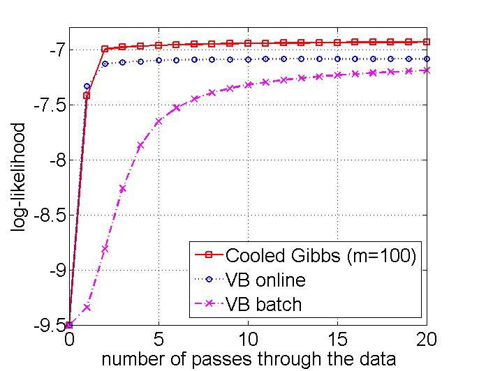
We first compare the convergence of SAME Gibbs LDA with other methods. We choose $m=100$ for the SAME sampler, because convergence speed only improves marginally beyond $m=100$, however, runtime per pass over the dataset starts to increase noticeably beyond $m=100$ while being relatively flat for $m<100$. The mini-batch size is set to be $1/20$ of the total number of examples. We use the per word log likelihood $ll=\frac{1}{N^{test}}\log(P(X^{test}))$ as a measure of convergence.

Figure 1 shows the cross-validated likelihood as a function of the number of passes through the data for both datasets, up to 20 passes. As we can see, the SAME Gibbs sampler converges to a higher quality result than VB online and VB batch on both datasets. The SAME sampler and VB online converged after 4-5 passes for the NYTimes dataset and 2 passes for the PubMed dataset. VB batch converges in about 20 passes.

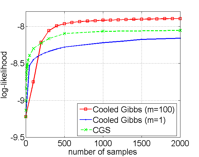
All three methods above are able to produce higher quality than CGS within 20 passes over the dataset. It usually takes 1000-2000 passes for CGS to converge for typical datasets such as NYTimes, as can be seen in Figure 1(c).

Figure 1(c) plots log-likelihood against the number of samples taken per word. We compare the SAME sampler with $m=100$, $m=1$ and CGS. To reach the same number of samples CGS and the SAME sampler with $m=1$ need to run 100 times as many passes over the data as the SAME sampler with $m=100$. That is Figure 1(c) shows 20 passes of SAME sampler with $m=100$ and 2000 passes of the other two methods. At the beginning, CGS converges faster. But in the long run, SAME Gibbs leads to better convergence. Notice that SAME with $m=1$ is not identical to CGS in our implementation, because of minibatching and the moving average estimate for $\Theta$.

(a) ll vs. n passes on NYTimes

(b) ll vs. n passes on PubMed

(c) ll vs. number of samples/word

Figure 1: Convergence Comparison

6.1.2 Runtime Performance

We further measure the runtime performance of different methods with different implementations for LDA. Again we fix the sample size for SAME GS at $m=100$. All the runtime number are generated by running each method/system on the NYTimes dataset with $K=256$, except that Yan’s parallel CGS [18] reports their benchmark for $K=128$. We also report time to convergence, which is defined as the time to reach the log-likelihood for standard CGS at the $1000^{th}$ iteration.

Table 1: Runtime Comparison on NYTimes

	SAME GS BIDMach	VB online BIDMach	VB batch BIDMach	VB batch Blei et al	CGS Griffiths et al	GPU CGS Yan et al
Runtime per pass (s)	30	20	20	12600	225	5.4
Time to converge (s)	90	40	400	252000	225000	5400

Results are illustrated in the Table 1. The SAME Gibbs sampler takes 90 seconds to converge on the NYTimes dataset. As comparison, the other CPU implementations take around 60-70 hours to converge, and Yan’s GPU implementation takes 5400 second to converge for $K=128$. Our system demonstrates two orders of magnitude improvement over the state of the art. Our implementation of online VB takes about 40 seconds to converge on the NYTimes dataset. The Gibbs sampling method is close in performance (less than a factor of 3) to that.

Finally, we compare our system with the state-of-art cluster implementation of CGS LDA [1], using time to convergence. Ahmed et al. [1] processed 200 million news articles on 100 machines and 1000 iterations in 2mins/iteration = 2000 minutes overall = 120k seconds. We constructed a repeating stream of news articles (as did [1]) and ran for two iterations - having found that this was sufficient for news datasets of comparable size. This took 30k seconds, which is 4x faster, on a single GPU node. Ahmed et al. also processed 2 billion articles on 1000 machines to convergence in 240k seconds, which is slightly less than linear scaling. Our system (which is sequential on minibatches) simply scales linearly to 300k seconds on this problem. Thus single-machine performance of GPU-accelerated SAME GS is almost as fast as a custom cluster CGS on 1000 nodes, and 4x faster than 100 nodes.

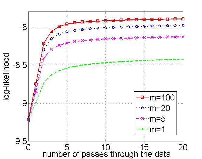
6.1.3 Multi-sampling and Annealing

The effect of sample number $m$ is studied in Figure 2 and Table 2. As expected, more samples yields better convergences given fixed number of passes through the data. And the benefit comes almost free thanks to the SIMD parallelism offered by the GPU. As shown in Table 2, $m=100$ is only modestly slower than $m=1$. However, the runtime for $m=500$ is much longer than $m=100$.

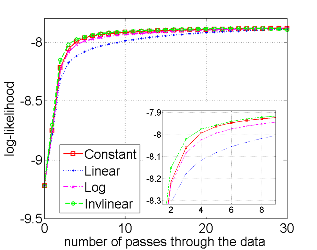
We next studied the effects of dynamic adjustment of $m$, i.e. annealing. We compare constant scheduling (fixed $m$) with

1. linear scheduling, $m_{t}=\frac{2mt}{t_{max}+1}$,

2. logarithmic scheduling, $m_{t}=mt_{max}\log t/\sum\limits_{t=1}^{t_{max}}\log t$,

3. invlinear scheduling, $m_{t}=\frac{2m(t_{max}+1-t)}{t_{max}+1}$.

$t_{max}$ is the total number of iterations. The average sample size per iteration is fixed to $m=100$ for all 4 configurations. As shown in Figure 2(b), we cannot identify any particular annealing schedule that is significantly better then fixed sample size. Invlinear is slighter faster at the beginning but has the highest initial sample number.

(a) ll vs. sample size m

(b) annealing schedule

Figure 2: Effect of sample sizes

Table 2: Runtime per iteration with different $m$

	m=500	m=100	m=20	m=5	m=1
Runtime per iteration (s)	50	30	25	23	20

7 Conclusions and Future Work

This paper described hardware-accelerated SAME Gibbs Parameter estimation - a method to improve and accelerate parameter estimation via Gibbs sampling. This approach reduces the number of passes over the dataset while introducing more parallelism into the sampling process. We showed that the approach meshes very well with SIMD hardware, and that a GPU-accelerated implementation of cooled GS for LDA is faster than other sequential systems, and comparable with the fastest cluster implementation of CGS on 1000 nodes. The code is at https://github.com/BIDData/BIDMach

SAME GS is applicable to many other problems, and we are currently exploring the method for inference on general graphical models. The coordinate-factored sampling approximation is also being applied to this problem in conjunction with full sampling (the approximation reduces the number of full samples required) and we anticipate similar large improvements in speed. The method provides the quality advantages of sampling and annealed estimation, while delivering performance with custom (symbolic) inference methods. We believe it will be the method of choice for many inference problems in future.

References

- [1] A. Ahmed, M. Aly, J. Gonzalez, S. Narayanamurthy, and A. J. Smola. Scalable inference in latent variable models. In Proceedings of the fifth ACM international conference on Web search and data mining, pages 123–132. ACM, 2012.
- [2] D. M. Blei, A. Y. Ng, and M. I. Jordan. Latent dirichlet allocation. the Journal of machine Learning research, 3:993–1022, 2003.
- [3] L. Bottou. Large-scale machine learning with stochastic gradient descent. In Proceedings of COMPSTAT’2010, pages 177–186. Springer, 2010.
- [4] L. Bottou and O. Bousquet. The tradeoffs of large scale learning. In NIPS, volume 4, page 2, 2007.
- [5] J. Canny and H. Zhao. Bidmach: Large-scale learning with zero memory allocation. In BigLearn Workshop, NIPS, 2013.
- [6] J. Canny and H. Zhao. Big data analytics with small footprint: Squaring the cloud. In Proceedings of the 19th ACM SIGKDD international conference on Knowledge discovery and data mining, pages 95–103. ACM, 2013.
- [7] A. P. Dempster, N. M. Laird, D. B. Rubin, et al. Maximum likelihood from incomplete data via the em algorithm. Journal of the Royal statistical Society, 39(1):1–38, 1977.
- [8] A. Doucet, S. Godsill, and C. Robert. Marginal maximum a posteriori estimation using markov chain monte carlo. Statistics and Computing, 12:77–84, 2002.
- [9] S. Geman and D. Geman. Stochastic relaxation, gibbs distributions, and the bayesian restoration of images. Pattern Analysis and Machine Intelligence, IEEE Transactions on, (6):721–741, 1984.
- [10] T. L. Griffiths and M. Steyvers. Finding scientific topics. Proceedings of the National academy of Sciences of the United States of America, 101(Suppl 1):5228–5235, 2004.
- [11] M. D. Hoffman, D. M. Blei, and F. R. Bach. Online learning for latent dirichlet allocation. In NIPS, volume 2, page 5, 2010.
- [12] M. I. Jordan, Z. Ghahramani, T. S. Jaakkola, and L. K. Saul. An introduction to variational methods for graphical models. Machine learning, 37(2):183–233, 1999.
- [13] T. Minka. Expectation propagation for approximate bayesian inference. 2001.
- [14] C. Robert, A. Doucet, and S. Godsill. Marginal MAP estimation using markov chain monte-carlo. In IEEE Int. Conf. on Acoustics, Speech and Signal Processing, volume 3, pages 1753–1756. IEEE, 1999.
- [15] G. C. Wei and M. A. Tanner. A monte carlo implementation of the em algorithm and the poor man’s data augmentation algorithms. Journal of the American Statistical Association, 85(411):699–704, 1990.
- [16] Y. Weiss. Correctness of local probability propagation in graphical models with loops. Neural Computation, 12(1):1–41, 2000.
- [17] J. Winn and C. Bishop. Variational message passing. Journal of Machine Learning Research, 6:661 V694, 2005.
- [18] F. Yan, N. Xu, and Y. Qi. Parallel inference for latent dirichlet allocation on graphics processing units. In NIPS, volume 9, pages 2134–2142, 2009.