Fused Lasso Additive Model

We consider the problem of predicting an outcome variable using $p$ covariates that are measured on $n$ independent observations, in the setting in which flexible and interpretable fits are desirable. We propose the fused lasso additive model (FLAM), in which each additive function is estimated to be piecewise constant with a small number of adaptively-chosen knots. FLAM is the solution to a convex optimization problem, for which a simple algorithm with guaranteed convergence to the global optimum is provided. FLAM is shown to be consistent in high dimensions, and an unbiased estimator of its degrees of freedom is proposed. We evaluate the performance of FLAM in a simulation study and on two data sets.

Keywords: additive model, feature selection, high-dimensional, non-parametric regression, piecewise constant, sparsity

1 Introduction

In this paper, we consider the task of predicting a response variable using $p$ features measured on $n$ independent observations. Approaches for this task typically offer either interpretability but limited flexibility (for instance, linear regression or a piecewise constant model with pre-specified knots) or flexibility but limited interpretability (for instance, a non-parametric approach). In this paper, we propose a method that balances the trade-off between interpretability and flexibility, while also allowing for sparsity in high dimensions when $p>n$. It selects a subset of features to include in the model, and for these features it fits piecewise constant functions with knots that are chosen adaptively based on the data.

We now introduce some notation. We let ${\bm{X}}$ denote an $n\times p$ matrix, for which ${\bm{x}}_{j}$ is the $j$th column (feature), and for which the $i$th element (observation) is $x_{ij}$. When we consider the case of $p=1$, we use ${\bm{x}}$ to denote the single feature, with $i$th element $x_{i}$. The response is an $n$-vector ${\bm{y}}$, with $i$th element $y_{i}$. To reference subvectors and submatrices, we use ${\bm{a}}_{\mathcal{S}}$ (${\bm{A}}_{\mathcal{S}}$) to denote ${\bm{a}}$ (${\bm{A}}$) with only the elements (columns) contained in the set $\mathcal{S}$.

The rest of this paper is organized as follows. In Section 2, we review related work. In Sections 3 and 4, we propose our method, present an algorithm to implement it, and examine some of its properties. Sections 5 and 6 contain the results of a simulation study and the analyses of two data sets. We consider some extensions in Section 7, and we close with a discussion in Section 8. Proofs are in the Appendix.

2 Previous Work

Generalized additive models (GAM) provide a flexible and general framework for modeling a response in low dimensions ($n>p$). We assume $\mbox{E}[y_{i}|{\bm{x}}_{i}]=g\left(\sum_{j=1}^{p}f_{j}(x_{ij})\right)$, where $g$ is a specified function and each $f_{j}$ is an unknown function that we wish to estimate (Hastie and Tibshirani, 1986). For now, we restrict our attention to the case when $g$ is the identity function. There are a number of ways to estimate $f_{j}$ — for example, we might use a smoothing or regression spline.

Flexible additive modeling in high dimensions has been an active area of research in recent years (Wood et al., 2014; Lin and Zhang, 2006; Avalos et al., 2007; Sardy and Tseng, 2004; Huang et al., 2010; Li and Liu, 2014; Zhang et al., 2011). Recently, Ravikumar et al. (2009) proposed a high-dimensional extension of GAM called sparse additive models (SpAM), which induces sparsity in the function estimates using a standardized group lasso penalty (Simon and Tibshirani, 2012). SpAM solves the problem

$$\underset{{\bm{\beta}}_{j}\in\mathbb{R}^{d},1\leq j\leq p}{\mathrm{minimize}}\quad\frac{1}{2n}\left\|{\bm{y}}-\sum_{j=1}^{p}\Psi_{j}{\bm{\beta}}_{j}\right\|_{2}^{2}+\lambda\sum_{j=1}^{p}\sqrt{\frac{1}{n}{\bm{\beta}}_{j}^{T}\Psi_{j}^{T}\Psi_{j}{\bm{\beta}}_{j}},$$ (1)

where ${\bm{\beta}}_{j}=\left(\beta_{j1}\cdots\beta_{jd}\right)^{T}$ is a $d$-vector of coefficients, and $\Psi_{j}=\left[\psi_{j1}\cdots\psi_{jd}\right]$ is an $n\times d$ matrix of which the columns are the $d$ basis functions used to model $f_{j}$.

Meier et al. (2009) modified (1) in order to obtain data-adaptive fits that can capture complex relationships if needed, but that otherwise are smooth. Their estimator is the solution to the optimization problem

$$\underset{{\bm{\beta}}_{j}\in\mathbb{R}^{d},1\leq j\leq p}{\mathrm{minimize}}\quad\frac{1}{n}\left\|{\bm{y}}-\sum_{j=1}^{p}\Psi_{j}{\bm{\beta}}_{j}\right\|_{2}^{2}+\lambda_{1}\sum_{j=1}^{p}\sqrt{\frac{1}{n}{\bm{\beta}}_{j}^{T}\Psi_{j}^{T}\Psi_{j}{\bm{\beta}}_{j}}+\lambda_{2}\sum_{j=1}^{p}\sqrt{{\bm{\beta}}_{j}^{T}{\bm{W}}_{j}{\bm{\beta}}_{j}},$$ (2)

where ${\bm{\beta}}_{j}=\left(\beta_{j1}\cdots\beta_{jd}\right)^{T}$ is a $d$-vector of coefficients to be estimated, $\Psi_{j}=\left[\psi_{j1}\cdots\psi_{jd}\right]$ is an $n\times d$ matrix of which the columns are the cubic B-spline basis vectors of the $j$th predictor, and ${\bm{W}}_{j}$ is a $d\times d$ matrix containing the inner products of the second derivatives of the cubic B-spline basis functions. Other variations of this sparsity-smoothness penalty have also been proposed (Meier et al., 2009; Bühlmann and Van De Geer, 2011).

Recently, Lou et al. (2014) proposed the sparse partially linear additive model, which models a subset of the included features linearly and the remaining included features non-linearly using basis functions. The linear features do not need to be chosen a priori.

3 The Fused Lasso Additive Model

The methods described in Section 2 rely on a pre-specified set of basis functions. This limits flexibility, since the basis functions must be chosen a priori rather than in a data-adaptive way, as well as interpretability, since for many choices of basis functions (e.g., natural cubic splines) the resulting fits can be complex and non-monotonic without clear change points.

We now propose an approach to fit an additive model in which each function is estimated to be piecewise constant with a small number of knots. While this problem is easily solved when the knots are chosen a priori, our proposal allows the knots to be chosen adaptively.

3.1 The Optimization Problem

To begin, we assume that we have a single feature ${\bm{x}}$ that is ordered, i.e., $x_{1}<x_{2}<\cdots<x_{n}$. We wish to estimate an $n$-vector ${\bm{\theta}}=(\theta_{1},\ldots,\theta_{n})$, where $\mbox{E}[y_{i}|x_{i}]=f(x_{i})=\theta_{i}$. The fused lasso seeks a piecewise constant estimate of ${\bm{\theta}}$ that involves a small number of knots, by solving the problem (Tibshirani et al., 2005)

$$\underset{{\bm{\theta}}\in\mathbb{R}^{n}}{\mathrm{minimize}}\quad\frac{1}{2}\left\|{\bm{y}}-{\bm{\theta}}\right\|_{2}^{2}+\lambda\left\|{\bm{D}}{\bm{\theta}}\right\|_{1},$$ (3)

where $\lambda\geq 0$ is a tuning parameter and ${\bm{D}}$ is the discrete first derivative matrix,

${\bm{D}}=\begin{pmatrix}1&-1&0&\cdots&0&0\\ 0&1&-1&\cdots&0&0\\ \vdots&&&&&\\ 0&0&0&\cdots&1&-1\end{pmatrix}$.

We let $\hat{\bm{\theta}}$ denote the solution to (3). The $\ell_{1}$ penalty encourages $\lvert\hat{\theta}_{i-1}-\hat{\theta}_{i}\rvert$ to equal zero when $\lambda$ is large. The non-zero elements of $\lvert\hat{\theta}_{i-1}-\hat{\theta}_{i}\rvert$ correspond to knots in $\hat{\bm{\theta}}$. Consequently, $\hat{\bm{\theta}}$ provides a piecewise constant fit to the data, with adaptively-chosen knots. Several algorithms for solving (3) have been proposed (Hoefling, 2010; Liu et al., 2010; Johnson, 2013).

We now consider the model $\mbox{E}[y_{i}|{\bm{x}}_{i}]=\sum_{j=1}^{p}f_{j}(x_{ij})=\sum_{j=1}^{p}\theta_{ji}$. We assume that each ${\bm{\theta}}_{j}$ is piecewise constant with mean zero, and we include an intercept $\theta_{0}$. Let ${\bm{P}}_{j}$ denote a permutation matrix that orders ${\bm{x}}_{j}$ from least to greatest. We can then solve the problem

$$\underset{\theta_{0}\in\mathbb{R},{\bm{\theta}}_{j}\in\mathbb{R}^{n},1\leq j\leq p}{\mathrm{minimize}}\quad\frac{1}{2}\left\|{\bm{y}}-\sum_{j=1}^{p}{\bm{\theta}}_{j}-\theta_{0}\bf{1}\right\|_{2}^{2}+\lambda\sum_{j=1}^{p}\left\|{\bm{D}}{\bm{P}}_{j}{\bm{\theta}}_{j}\right\|_{1}\quad\text{subject to }{\bm{1}}^{T}{\bm{\theta}}_{j}={\bm{0}}\quad\forall j.$$ (4)

In high dimensions, we may wish to impose sparsity on the ${\bm{\theta}}_{j}$’s, so that a given feature is completely excluded from the model. For $\lambda$ sufficiently large, we do get a sparse solution in (4), but this value of $\lambda$ will tend to overshrink all of the estimates for ${\bm{\theta}}_{j}$. Therefore, we consider the modified optimization problem

$$\underset{\theta_{0}\in\mathbb{R},{\bm{\theta}}_{j}\in\mathbb{R}^{n},1\leq j\leq p}{\mathrm{minimize}}\quad\frac{1}{2}\left\|{\bm{y}}-\sum_{j=1}^{p}{\bm{\theta}}_{j}-\theta_{0}\bf{1}\right\|_{2}^{2}+\alpha\lambda\sum_{j=1}^{p}\left\|{\bm{D}}{\bm{P}}_{j}{\bm{\theta}}_{j}\right\|_{1}+(1-\alpha)\lambda\sum_{j=1}^{p}\left\|{\bm{\theta}}_{j}\right\|_{2},$$ (5)

where $\lambda\geq 0$ and $0\leq\alpha\leq 1$. Here, $\alpha$ provides a trade-off between encouraging $\hat{\bm{\theta}}_{j}$ to be piecewise constant, and inducing sparsity on the entire vector $\hat{\bm{\theta}}_{j}$ using the group lasso (Yuan and Lin, 2006). We refer to the solution to (5) as the fused lasso additive model (FLAM).

3.2 An Algorithm for FLAM

Problem 5 is convex, and so can be solved using a general-purpose interior point method that has a per-iteration computational complexity of $\mathcal{O}(n^{3}p^{3})$. Here we develop a much faster algorithm using block coordinate descent to solve (5) (Tseng, 2001). We cycle through the features and repeatedly perform a partial minimization in a single ${\bm{\theta}}_{j}$, holding all others fixed. The solution for the partial minimization is given in Corollary 3.1, which follows from a more general result presented in Section 7.3. This corollary allows us to solve the FLAM optimization problem in $\mathcal{O}(n)$ operations per feature per iteration, by leveraging an existing fused lasso solver that requires $\mathcal{O}(n)$ operations for an $n$-dimensional problem (Johnson, 2013).

Corollary 3.1

The solution to the optimization problem

$$\underset{{\bm{\theta}}\in\mathbb{R}^{n}}{\mathrm{minimize}}\quad\frac{1}{2}\left\|{\bm{y}}-{\bm{\theta}}\right\|_{2}^{2}+\alpha\lambda\left\|{\bm{D}}{\bm{\theta}}\right\|_{1}+(1-\alpha)\lambda\left\|{\bm{\theta}}\right\|_{2}$$ (6)

is $\left(1-\frac{(1-\alpha)\lambda}{\left\|\hat{\bm{\theta}}\right\|_{2}}\right)_{+}\hat{\bm{\theta}}$,  where $(u)_{+}=\max(u,0)$ and $\hat{\bm{\theta}}$ is the solution to

$$\underset{{\bm{\theta}}\in\mathbb{R}^{n}}{\mathrm{minimize}}\quad\frac{1}{2}\left\|{\bm{y}}-{\bm{\theta}}\right\|_{2}^{2}+\alpha\lambda\left\|{\bm{D}}{\bm{\theta}}\right\|_{1}.$$ (7)

Corollary 3.1 leads directly to Algorithm 1, which yields the global optimum to (5) (Tseng, 2001), and can be made very efficient using warm starts and active sets.

Algorithm 1 — Block Coordinate Descent for Fused Lasso Additive Model (Equation 5)

1. Initialize $\hat{\theta}_{0}=0$ and $\hat{\bm{\theta}}_{j}=\mathbf{0}$ for all $j=1,\ldots,p$.

2. For each $j=1,\ldots,p$, perform the following:

   • Compute the residual ${\bm{r}}_{j}={\bm{y}}-\hat{\theta}_{0}{\bf 1}-\sum_{j^{\prime}\neq j}\hat{\bm{\theta}}_{j^{\prime}}$.

   • Using an algorithm for the fused lasso (e.g., flsa on CRAN (Hoefling, 2013)), solve

     $\displaystyle\underset{{\bm{\theta}}_{j}\in\mathbb{R}^{n}}{\mathrm{minimize}}\quad\frac{1}{2}\left\|\bm{r}_{j}-{\bm{\theta}}_{j}\right\|_{2}^{2}+\alpha\lambda\left\|{\bm{D}}{\bm{P}}_{j}{\bm{\theta}}_{j}\right\|_{1}$.

   • Compute the intercept, $\hat{\theta}_{0}\leftarrow\hat{\theta}_{0}+\text{mean}(\hat{\bm{\theta}}_{j})$, and center, $\hat{\bm{\theta}}_{j}\leftarrow\hat{\bm{\theta}}_{j}-\text{mean}(\hat{\bm{\theta}}_{j})$.

   • Soft-scale the estimate: $\hat{\bm{\theta}}_{j}\leftarrow\left(1-\frac{(1-\alpha)\lambda}{\left\|\hat{\bm{\theta}}_{j}\right\|_{2}}\right)_{+}\hat{\bm{\theta}}_{j}$ where $(u)_{+}=\max(u,0).$

3. Repeat Step 2 until convergence of the objective of (5).

3.3 Connections to Other Methods

The fused lasso can be interpreted as $\ell_{1}$ trend filtering with order $k=0$ (Kim et al., 2009; Tibshirani, 2014). Tibshirani (2014) showed that 0th order trend filtering is equivalent to 0th order locally adaptive regression splines, proposed by Mammen et al. (1997). Therefore, we can interpret FLAM with $\alpha=1$ as a multi-variable extension of locally adaptive regression splines. Indeed, we illustrate FLAM’s local adaptivity, or ability to produce a fit that is highly variable in one portion of the domain and constant in another, in Section 5.

When $\alpha=0$, FLAM is equivalent to SpAM with $\Psi_{j}={\bm{I}}\in\mathbb{R}^{n\times n}$ in (1). However, this is an impractical special case in which the design matrix does not depend on the covariates.

4 Properties of FLAM

We define $\tilde{\bm{y}}={\bm{y}}-\frac{1}{n}{\bm{1}}^{T}{\bm{y}}{\bm{1}}$ and ${\bm{V}}=[{\bm{P}}_{1}^{T}{\bm{U}}\cdots{\bm{P}}_{p}^{T}{\bm{U}}]$, where ${\bm{U}}\in\mathbb{R}^{n\times(n-1)}$ is the matrix obtained by centering the columns of the upper triangular matrix of 1’s, and removing the $n$th column. The following lemma indicates that FLAM can be reparameterized in terms of the pairwise differences among the ordered elements of ${\bm{\theta}}_{j}$ (i.e., the elements of ${\bm{\beta}}_{j}={\bm{D}}{\bm{P}}_{j}{\bm{\theta}}_{j}$).

Lemma 4.1

Let $\hat{\bm{\beta}}=(\hat{\bm{\beta}}_{1}^{T}\;\cdots\;\hat{\bm{\beta}}_{p}^{T})^{T}$ be the solution to

$$\underset{{\bm{\beta}}\in\mathbb{R}^{(n-1)p}}{\mathrm{minimize}}\quad\frac{1}{2}\left\|\tilde{\bm{y}}-{\bm{V}}{\bm{\beta}}\right\|_{2}^{2}+\alpha\lambda\left\|{\bm{\beta}}\right\|_{1}+(1-\alpha)\lambda\sum_{j=1}^{p}\left\|{\bm{U}}{\bm{\beta}}_{j}\right\|_{2}.$$ (8)

Then the solution $\hat{\theta}_{0},\hat{\bm{\theta}}_{1},\ldots,\hat{\bm{\theta}}_{p}$ to the optimization problem (5) is

$$\hat{\theta}_{0}=\frac{1}{n}{\bm{1}}^{T}{\bm{y}}\text{ and }\hat{\bm{\theta}}_{j}={\bm{P}}_{j}^{T}{\bm{U}}\hat{\bm{\beta}}_{j}\text{ for }j=1,\ldots,p.$$

From (8), FLAM with $\alpha=1$ is equivalent to solving a lasso problem. The reparametrization given in Lemma 4.1 will allow us to easily derive some properties of FLAM.

4.1 Degrees of Freedom for FLAM

Suppose that ${\bm{y}}\sim({\bm{\mu}},\sigma^{2}{\bm{I}})$, and let $g({\bm{y}})=\hat{{\bm{y}}}$ denote the fit corresponding to some model-fitting procedure $g$. Then the degrees of freedom of $g$ is defined as $\frac{1}{\sigma^{2}}\sum_{i=1}^{n}\mbox{Cov}(y_{i},\hat{y}_{i})$ (Hastie and Tibshirani, 1990; Efron, 1986). We now consider a modified version of FLAM, in which a small ridge penalty ensures strict convexity and enforces uniqueness of the solution,

$$\underset{\theta_{0}\in\mathbb{R},{\bm{\theta}}_{j}\in\mathbb{R}^{n},1\leq j\leq p}{\mathrm{minimize}}\quad\frac{1}{2}\left\|{\bm{y}}-\sum_{j=1}^{p}{\bm{\theta}}_{j}-\theta_{0}\bf{1}\right\|_{2}^{2}+\alpha\lambda\sum_{j=1}^{p}\left\|{\bm{D}}{\bm{P}}_{j}{\bm{\theta}}_{j}\right\|_{1}+(1-\alpha)\lambda\sum_{j=1}^{p}\left\|{\bm{\theta}}_{j}\right\|_{2}+\frac{\epsilon}{2}\sum_{j=1}^{p}\|{\bm{D}}{\bm{P}}_{j}{\bm{\theta}}_{j}\|_{2}^{2}.$$ (9)

In (9), $\epsilon\geq 0$ is a very small constant. Subject to reparameterization, (9) is equivalent to

$$\underset{{\bm{\beta}}\in\mathbb{R}^{(n-1)p}}{\mathrm{minimize}}\quad\frac{1}{2}\left\|\tilde{\bm{y}}-{\bm{V}}{\bm{\beta}}\right\|_{2}^{2}+\alpha\lambda\left\|{\bm{\beta}}\right\|_{1}+(1-\alpha)\lambda\sum_{j=1}^{p}\left\|{\bm{U}}{\bm{\beta}}_{j}\right\|_{2}+\frac{\epsilon}{2}\sum_{j=1}^{p}\|{\bm{\beta}}_{j}\|_{2}^{2}.$$ (10)

We propose to estimate the degrees of freedom of FLAM as

$$\hat{df}_{FLAM}=\mbox{Tr}\left({\bm{V}}_{\mathcal{A}}\left[{\bm{V}}_{\mathcal{A}}^{T}{\bm{V}}_{\mathcal{A}}+(1-\alpha)\lambda S_{2}+\epsilon{\bm{I}}\right]^{-1}{\bm{V}}_{\mathcal{A}}^{T}\right)+1,$$ (11)

where $\mathcal{A}=\{i\in\{1,\ldots,(n-1)p\}:\hat{\beta}_{i}\neq 0\}$ and $S_{2}$ is block diagonal with the $j$th block equal to $\frac{{\bm{U}}_{\mathcal{A}_{j}}^{T}{\bm{U}}_{\mathcal{A}_{j}}}{\|{\bm{U}}_{\mathcal{A}_{j}}\hat{\bm{\beta}}_{j\mathcal{A}_{j}}\|_{2}}-\frac{{\bm{U}}_{\mathcal{A}_{j}}^{T}{\bm{U}}_{\mathcal{A}_{j}}\hat{\bm{\beta}}_{j\mathcal{A}_{j}}\hat{\bm{\beta}}_{j\mathcal{A}_{j}}^{T}{\bm{U}}_{\mathcal{A}_{j}}^{T}{\bm{U}}_{\mathcal{A}_{j}}}{\|{\bm{U}}_{\mathcal{A}_{j}}\hat{\bm{\beta}}_{j\mathcal{A}_{j}}\|_{2}^{3}}$ with $\mathcal{A}_{j}=\{i\in\{1,\ldots,n-1\}:\hat{\beta}_{ji}\neq 0\}$.

Proposition 4.2

Assume ${\bm{y}}\sim MVN({\bm{\mu}},\sigma^{2}{\bm{I}})$. Then $\hat{df}_{FLAM}$ is an unbiased estimator of the degrees of freedom of FLAM.

When $\alpha=1$ and $\epsilon=0$, (11) reduces to $\text{rank}({\bm{V}}_{\mathcal{A}})+1$, which agrees with the estimator proposed in Tibshirani et al. (2012). Recall that $\hat{\bm{\beta}}_{j}={\bm{D}}{\bm{P}}_{j}\hat{\bm{\theta}}_{j}$, so $\hat{\beta}_{ji}$ is the difference between $[{\bm{P}}_{j}\hat{\bm{\theta}}_{j}]_{i-1}$ and $[{\bm{P}}_{j}\hat{\bm{\theta}}_{j}]_{i}$. Thus non-zero elements of $\hat{\bm{\beta}}$ correspond to knots in the estimated fits. When ${\bm{V}}_{\mathcal{A}}$ is full rank (which only occurs when the number of knots is smaller than $n$), the following corollary provides a simple estimator for FLAM’s degrees of freedom.

Corollary 4.3

Suppose that ${\bm{V}}_{\mathcal{A}}$ is full rank, and let $\alpha=1$ in (9). Then the degrees of freedom of FLAM is one greater than the total number of knots across all estimated fits.

In 1000 replicate data sets, we compare the mean of (11) to the mean of

$$\frac{1}{\sigma^{2}}\sum_{i=1}^{n}\left(\hat{y}_{i}-\mu_{i}\right)\left(y_{i}-\mu_{i}\right),$$ (12)

which is an estimator of $\frac{1}{\sigma^{2}}\sum_{i=1}^{n}\mbox{Cov}(y_{i},\hat{y}_{i})$. Data are generated according to the high-dimensional setting of scenario 1, described in Section 5. Results are displayed in Figure 1(a).

We also propose an estimator for the degrees of freedom of SpAM (1). Defining $\Psi=\left[\Psi_{1}\cdots\Psi_{d}\right]$ and ${\bm{\beta}}=\left({\bm{\beta}}_{1}^{T}\cdots{\bm{\beta}}_{d}^{T}\right)^{T}$, we estimate SpAM’s degrees of freedom as

$$\hat{df}_{SpAM}=\mbox{Tr}\left(\Psi_{\mathcal{A}}\left[\Psi_{\mathcal{A}}^{T}\Psi_{\mathcal{A}}+\lambda D_{2}\right]^{-1}\Psi_{\mathcal{A}}^{T}\right),$$ (13)

where $\mathcal{A}=\{i\in\{1,\ldots,pd\}:\hat{\beta}_{i}\neq 0\}$ and $D_{2}$ is block diagonal with the $j$th block equal to $\frac{\Psi_{j\mathcal{A}_{j}}^{T}\Psi_{j\mathcal{A}_{j}}}{\|\Psi_{j\mathcal{A}_{j}}\hat{\bm{\beta}}_{j\mathcal{A}_{j}}\|_{2}}-\frac{\Psi_{j\mathcal{A}_{j}}^{T}\Psi_{j\mathcal{A}_{j}}\hat{\bm{\beta}}_{j\mathcal{A}_{j}}\hat{\bm{\beta}}_{j\mathcal{A}_{j}}^{T}\Psi_{j\mathcal{A}_{j}}^{T}\Psi_{j\mathcal{A}_{j}}}{\|\Psi_{j\mathcal{A}_{j}}\hat{\bm{\beta}}_{j\mathcal{A}_{j}}\|_{2}^{3}}$ with $\mathcal{A}_{j}=\{i\in\{1,\ldots,d\}:\hat{\beta}_{ji}\neq 0\}$.

Proposition 4.4

Assume ${\bm{y}}\sim MVN({\bm{\mu}},\sigma^{2}{\bm{I}})$. Then $\hat{df}_{SpAM}$ is an unbiased estimator of the degrees of freedom of SpAM.

Interestingly, Ravikumar et al. (2009) proposed

$$\sum_{j=1}^{p}\sum_{k=1}^{d}I\left(\hat{\beta}_{jk}\neq 0\right)$$ (14)

as an estimator for SpAM’s degrees of freedom. Figure 1(b) compares the means of the two estimators (13) and (14) with the mean of (12) across 1000 replicate data sets. In fact, we see that (13) is far more accurate than (14).

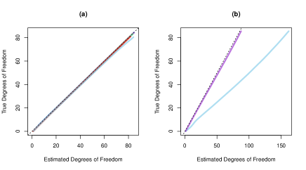
Figure 1: In (a), we compare the degrees of freedom of FLAM calculated using (12) (y-axis) to the unbiased estimator (11) (x-axis) for $\alpha=\{0,0.2,0.4,0.6,0.8,1\}$; each value of $\alpha$ is indicated by an (overlapping) colored line. In (b), we compare the degrees of freedom for SpAM with $d=3$ calculated using (12) (y-axis) to the estimators (13) () and (14) () (x-axis). In both plots, the solid lines are obtained by varying $\lambda$ for FLAM or SpAM. The black dotted lines indicate $y=x$.

4.2 Range of $\lambda$ that Yields Complete Sparsity

We now consider the range of $\lambda$ for which $\hat{\bm{\theta}}_{j}={\bm{0}}$ for $j=1,\ldots,p$, for $\alpha=1$ and $\alpha=0$.

Lemma 4.5

If $\alpha=1$, then the solution to (5) is completely sparse if and only if $\lambda\geq\|{\bm{V}}^{T}\tilde{\bm{y}}\|_{\infty}$. If $\alpha=0$, then the solution is completely sparse if and only if $\lambda\geq\|\tilde{\bm{y}}\|_{2}$.

In Lemma 4.5, note that $\|{\bm{V}}^{T}\tilde{\bm{y}}\|_{\infty}=\max\left(g({\bm{P}}_{1}\tilde{\bm{y}}),\ldots,g({\bm{P}}_{p}\tilde{\bm{y}})\right)$, where $g({\bm{a}})=\max\{\lvert a_{1}\rvert,\lvert a_{1}+a_{2}\rvert,\ldots,\lvert a_{1}+a_{2}+\ldots+a_{n-1}\rvert\}$. We now present a sufficient condition for the FLAM solution to be completely sparse, for any $\alpha$.

Corollary 4.6

For any $\alpha\in[0,1]$, if $\lambda\geq\min\left(\frac{\|{\bm{V}}^{T}\tilde{\bm{y}}\|_{\infty}}{\alpha},\frac{\|\tilde{\bm{y}}\|_{2}}{1-\alpha}\right)$, then the solution to (5) is completely sparse.

When selecting $\lambda$ for FLAM, we need never consider a value larger than that in Corollary 4.6.

4.3 Prediction Consistency

In this section, we establish prediction consistency for FLAM. For simplicity, we assume ${\bm{y}}$ has mean zero in this subsection. The estimated prediction error compares the predicted outcome to the best one could do if the true coefficient values ${\bm{\theta}}_{1}^{0},\ldots,{\bm{\theta}}_{p}^{0}$ were known. Lemma 4.7 provides a finite sample bound for the prediction error.

Lemma 4.7

Assume ${\bm{y}}=\sum_{j=1}^{p}{\bm{\theta}}_{j}^{0}+{\bm{\epsilon}}$ with ${\bm{\epsilon}}\sim MVN({\bm{0}},\sigma^{2}{\bm{I}})$. If $\lambda\geq 2\sigma\sqrt{\frac{\log((n-1)p)}{n}}$, then

$$\frac{1}{n}\left\|\sum_{j=1}^{p}\left(\hat{\bm{\theta}}_{j}-{\bm{\theta}}_{j}^{0}\right)\right\|^{2}_{2}\leq 3\lambda\sum_{j=1}^{p}\left[\alpha\left\|{\bm{D}}{\bm{P}}_{j}{\bm{\theta}}^{0}_{j}\right\|_{1}+(1-\alpha)\|{\bm{\theta}}_{j}^{0}\|_{2}\right]$$

holds with probability at least $1-\left(\frac{2}{(n-1)p}+\frac{1}{n}\right)$.

Now, assume that $\theta_{ji}^{0}=f_{j}(x_{ij})$ where $f_{j}$ has bounded variation, and all elements of ${\bm{x}}_{j}\in[a,b]$ for some $a$ and $b$. Assume also that the number of non-sparse functions is bounded, i.e., $\sum_{j=1}^{p}||f_{j}||_{0}=K<\infty$. Together, these two assumptions imply that $\sum_{j=1}^{p}\|{\bm{D}}{\bm{P}}_{j}{\bm{\theta}}_{j}^{0}\|_{1}=O(1)$, and that $\sum_{j=1}^{p}\|{\bm{\theta}}_{j}^{0}\|_{2}=O(\sqrt{n})$. Thus, FLAM is prediction consistent provided that $(1-\alpha)=o((\log((n-1)p))^{-1/2})$, and $\lambda=2\sigma\sqrt{\frac{\log((n-1)p)}{n}}$.

5 Simulations

We compare the performance of FLAM to two competitors: GAM using smoothing splines (implemented with the R package gam (Hastie, 2013)), and SpAM with basis vectors corresponding to a natural cubic spline with $d-1$ non-boundary knots at equally spaced quantiles of ${\bm{x}}_{j}$ (implemented with the R package SAM (Zhao et al., 2014)). Data are generated according to $y_{i}=\sum_{j=1}^{p}f_{j}(x_{ij})+\epsilon_{i}$ with $\epsilon_{i}\stackrel{{\scriptstyle iid}}{{\sim}}N(0,1)$, $x_{ij}\stackrel{{\scriptstyle iid}}{{\sim}}\text{Uniform}[-2.5,2.5]$, and $p=4$. We consider four scenarios, displayed in Figure 2:

1. Scenario 1: All $f_{j}$ are piecewise constant functions (Figure 2(a)).

2. Scenario 2: All $f_{j}$ are smooth functions (Figure 2(b)). These are the exact functions used for the simulations in the original SpAM paper (Ravikumar et al., 2009).

3. Scenario 3: Two of the $f_{j}$ are piecewise constant functions and the other two $f_{j}$ are smooth functions (Figure 2(c)). This is a compromise between scenarios 1 and 2.

4. Scenario 4: All $f_{j}$ are functions that are constant in some areas of the domain and highly variable in other areas of the domain (Figure 2(d)).

All functions are constructed such that $\int_{-2.5}^{2.5}f_{j}=0$ and $\int_{-2.5}^{2.5}f_{j}^{2}=1$. We refer to scenarios 1-4 as the low-dimensional setting. Additionally, we refer to the same scenarios with the addition of 96 noise functions (i.e., $f_{5},\ldots,f_{100}=0$) as the high-dimensional setting. We note that GAM can only be applied in the low-dimensional setting ($n>p$).

Figure 2: Functions used to generate data in: (a) scenario 1, (b) scenario 2, (c) scenario 3, and (d) scenario 4.

For each scenario, we generate training, test, and validation sets, each with $n=100$. Functions are fit on the training set, and mean squared error $\left(\textrm{MSE; }\frac{1}{n}\left\|{\bm{y}}-\hat{\bm{y}}\right\|_{2}^{2}\right)$ is evaluated on the test set. For FLAM, we fix $\alpha=0.5,0.75,\text{ or }1$ and consider a range of $\lambda$. For GAM, we consider a range of degrees of freedom for each smoothing spline, from 1 (just a linear fit) to $n/p$. For SpAM, we fix $d=3,6,\text{ or }10$ and consider a range of $\lambda$.

We evaluate each method’s performance as a function of its degrees of freedom. For GAM, the total degrees of freedom is $p$ multiplied by the degrees of freedom for each covariate’s smoothing spline, plus one degree of freedom for the intercept. For FLAM and SpAM, the degrees of freedom are estimated using (11) and (13), respectively.

Figure 3 displays the test set MSE versus total degrees of freedom for the three methods. FLAM achieves the lowest test set MSE across all scenarios except in scenario 2 where all $f_{j}$ are smooth. GAM performs comparably to SpAM in scenario 3 without noise functions. As expected, FLAM with $\alpha=1$ outperforms FLAM with $\alpha<1$ in the scenarios without noise functions, as no additional sparsity is needed. In general, $\alpha<1$ is preferred in the scenarios with noise functions, with the exception of scenario 4. We discuss this discrepancy below.

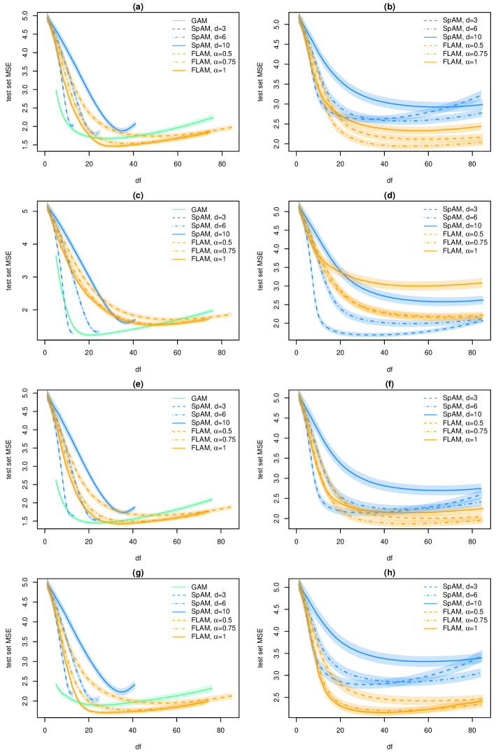
Figure 3: Mean test set MSE plotted by degrees of freedom (df) for: (a) scenario 1, (b) scenario 1 with noise functions, (c) scenario 2, (d) scenario 2 with noise functions, (e) scenario 3, (f) scenario 3 with noise functions, (g) scenario 4, and (h) scenario 4 with noise functions. Shaded bands indicate point-wise 95% confidence intervals over the 100 replicate data sets. GAM is only applicable in the low-dimensional setting.

Additionally, we summarize performance for the optimal tuning parameter, defined as the tuning parameter corresponding to the minimum test set MSE. We calculate the validation set MSE for the training set fit corresponding to the optimal tuning parameter, as well as the parameter fit $(\sum_{j=1}^{p}\|{\bm{\theta}}_{j}-\hat{\bm{\theta}}_{j}\|_{2}^{2})$, sparsity, and degrees of freedom (Table 1). Once again, FLAM performs best in all scenarios except when all $f_{j}$ are smooth (scenario 2), with the best performance corresponding to FLAM with $\alpha=1$ in the low-dimensional setting and $\alpha=0.75$ in the high-dimensional setting. In scenario 4 with noise functions, FLAM with $\alpha=1$ is able to achieve comparable sparsity to FLAM with $\alpha<1$. This explains the optimal performance of FLAM with $\alpha=1$ in this setting (Figure 3).

Table 1: Results on the validation data, with the tuning parameter value chosen based on test set MSE. Mean (standard error) across 100 replicate data sets are shown. Parameter fit is defined as $\sum_{j=1}^{p}\left\|{\bm{\theta}}_{j}-\hat{\bm{\theta}}_{j}\right\|_{2}^{2}$. Note that GAM can only be applied in the low-dimensional setting. All $\hat{f}_{j}$ were non-zero for all methods in the low-dimensional setting.

	Low-dimensional			High-dimensional
		Parameter	Degrees of		Parameter	Proportion	Degrees of
	MSE	fit	freedom	MSE	fit	$\hat{f}_{j}$ non-zero	freedom
Scenario 1
FLAM, $\alpha=0.5$	1.73 (0.03)	75.6 (1.8)	51.0 (1.1)	2.11 (0.05)	113.0 (3.3)	0.20 (0.01)	61.6 (1.5)
FLAM, $\alpha=0.75$	1.52 (0.03)	55.4 (1.5)	39.0 (1.0)	1.92 (0.04)	95.0 (2.9)	0.23 (0.01)	54.0 (1.5)
FLAM, $\alpha=1$	1.45 (0.02)	48.2 (1.4)	32.7 (0.8)	2.30 (0.06)	132.7 (3.4)	0.35 (0.01)	58.8 (1.9)
GAM	1.67 (0.02)	65.1 (1.3)	28.7 (0.9)
SpAM, $d=3$	2.02 (0.03)	107.5 (1.4)	12.2 (0.1)	2.54 (0.05)	162.0 (2.6)	0.23 (0.01)	36.7 (1.3)
SpAM, $d=6$	1.79 (0.03)	110.0 (3.0)	22.7 (0.2)	2.52 (0.05)	168.2 (3.3)	0.23 (0.01)	50.7 (1.5)
SpAM, $d=10$	1.85 (0.03)	130.5 (3.3)	35.4 (0.3)	2.91 (0.06)	208.9 (4.1)	0.24 (0.01)	66.5 (1.6)
Scenario 2
FLAM, $\alpha=0.5$	1.66 (0.03)	69.1 (1.9)	60.0 (1.1)	2.14 (0.05)	112.6 (3.4)	0.22 (0.01)	71.4 (1.5)
FLAM, $\alpha=0.75$	1.51 (0.02)	56.1 (1.4)	52.9 (0.9)	2.17 (0.05)	115.8 (3.4)	0.27 (0.01)	66.5 (1.6)
FLAM, $\alpha=1$	1.46 (0.02)	52.8 (1.3)	50.2 (0.9)	2.94 (0.06)	192.5 (4.1)	0.36 (0.01)	60.9 (2.3)
GAM	1.19 (0.02)	23.3 (0.7)	21.6 (0.4)
SpAM, $d=3$	1.21 (0.02)	32.9 (1.3)	12.5 (0.1)	1.65 (0.03)	70.3 (2.3)	0.23 (0.01)	37.4 (1.5)
SpAM, $d=6$	1.27 (0.02)	54.6 (2.1)	23.6 (0.1)	1.95 (0.05)	109.7 (3.6)	0.23 (0.01)	53.0 (1.5)
SpAM, $d=10$	1.50 (0.03)	84.1 (2.4)	37.1 (0.2)	2.55 (0.06)	168.3 (4.6)	0.25 (0.01)	68.6 (1.5)
Scenario 3
FLAM, $\alpha=0.5$	1.63 (0.03)	66.8 (1.6)	51.8 (1.1)	1.98 (0.04)	101.2 (3.3)	0.20 (0.01)	61.6 (1.5)
FLAM, $\alpha=0.75$	1.45 (0.02)	49.2 (1.3)	40.2 (0.9)	1.84 (0.04)	88.1 (2.7)	0.24 (0.01)	54.9 (1.6)
FLAM, $\alpha=1$	1.38 (0.02)	43.7 (1.3)	36.5 (0.8)	2.12 (0.04)	115.2 (3.1)	0.31 (0.01)	55.0 (2.1)
GAM	1.44 (0.02)	44.2 (1.0)	24.1 (0.7)
SpAM, $d=3$	1.62 (0.02)	69.0 (1.4)	12.2 (0.1)	2.09 (0.04)	115.3 (2.7)	0.23 (0.01)	35.1 (1.3)
SpAM, $d=6$	1.51 (0.02)	73.3 (2.4)	22.9 (0.1)	2.18 (0.04)	134.4 (3.5)	0.23 (0.01)	50.6 (1.3)
SpAM, $d=10$	1.68 (0.03)	103.7 (3.1)	35.7 (0.2)	2.68 (0.05)	188.3 (4.2)	0.24 (0.01)	66.7 (1.6)
Scenario 4
FLAM, $\alpha=0.5$	1.91 (0.04)	91.4 (1.9)	55.6 (1.3)	2.38 (0.05)	137.1 (3.2)	0.21 (0.01)	61.5 (1.9)
FLAM, $\alpha=0.75$	1.73 (0.03)	74.5 (1.6)	42.9 (1.2)	2.15 (0.04)	115.4 (2.6)	0.21 (0.01)	45.8 (1.7)
FLAM, $\alpha=1$	1.64 (0.03)	67.2 (1.5)	33.8 (1.3)	2.13 (0.03)	112.1 (2.4)	0.25 (0.01)	43.1 (1.6)
GAM	1.88 (0.03)	82.2 (1.4)	28.5 (1.6)
SpAM, $d=3$	2.15 (0.03)	121.2 (2.0)	12.2 (0.1)	2.75 (0.05)	176.2 (3.2)	0.21 (0.01)	32.9 (1.2)
SpAM, $d=6$	2.01 (0.03)	120.6 (2.6)	22.6 (0.2)	2.78 (0.05)	187.8 (3.9)	0.24 (0.01)	51.3 (1.7)
SpAM, $d=10$	2.19 (0.04)	157.1 (3.5)	35.0 (0.3)	3.23 (0.06)	237.4 (4.4)	0.22 (0.01)	60.0 (1.8)

A strength of FLAM is its local adaptivity, or ability to produce a fit that is highly variable in one portion of the domain and constant in another. We can see this qualitatively by examining the function fits for scenario 4 with 96 noise functions. In Figure 4, we plot the fits corresponding to the the optimal tuning parameter (as defined above) for the truly non-zero functions, across 25 replicate data sets. In general, FLAM more adeptly fits both the constant and highly variable regions of the functions, relative to SpAM. SpAM’s local adaptivity is limited due to the types of penalties imposed in (1) — $\lambda$ encourages the entire $\hat{f}_{j}$ to be zero, while $d$ controls the amount of flexibility in each $\hat{f}_{j}$. Having fewer basis functions (i.e., small $d$) results in less variable function fits, while a large $d$ can produce highly variable function fits. However, the amount of variability cannot be varied greatly over the domain of the function fit, unless basis functions are specifically chosen for this purpose a priori.

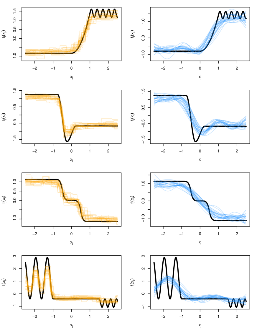
Figure 4: We compare the fits of FLAM () and SpAM () with the true underlying functions () generated according to scenario 4. In each panel, 25 curves are shown. Each curve corresponds to a validation set fit with the optimal tuning parameter value, over one simulated data set.

6 Data Application

6.1 Predictors of a Country’s Happiness

We now consider whether wealth is associated with happiness, by estimating the conditional relationships between a country-level happiness index and gross national income, as well as 11 other country-level predictors. The happiness index is the average of Cantril Scale (Cantril, 1965) responses of approximately 3000 residents in each country obtained in Gallup World Polls from 2010-2012, publicly available from the United Nations (UN) 2013 World Happiness Report (Helliwell et al., 2013). The predictors are publicly available through the UN Human Development Reports and the World Bank Development Indicators (World Bank Group, 2012; UNDP, 2012). They are from 2012 data or the closest year prior.

We consider 10 splits of the 109 countries with complete data into training and test sets. We compare FLAM to GAM with an identity link and smoothing splines using the R package gam (Hastie, 2013). Tuning parameters are chosen using 10-fold CV in the training set. The estimated fits are shown in Figure 5. Both methods provide a large improvement in average test set MSE across 10 splits of the data (FLAM: 0.367; GAM: 0.308) compared to the intercept-only model (1.19). FLAM’s estimated fits are both intuitive and fairly similar across the different splits of data. Conditional on the other predictors, FLAM estimates that increased gross national income is associated with increased happiness, up to a certain level of income. Beyond that, happiness is constant. We were quite surprised to see that GAM finds a negative conditional association between a country’s happiness index and the number of scientific journal publications. Reassuringly, FLAM found no such association.

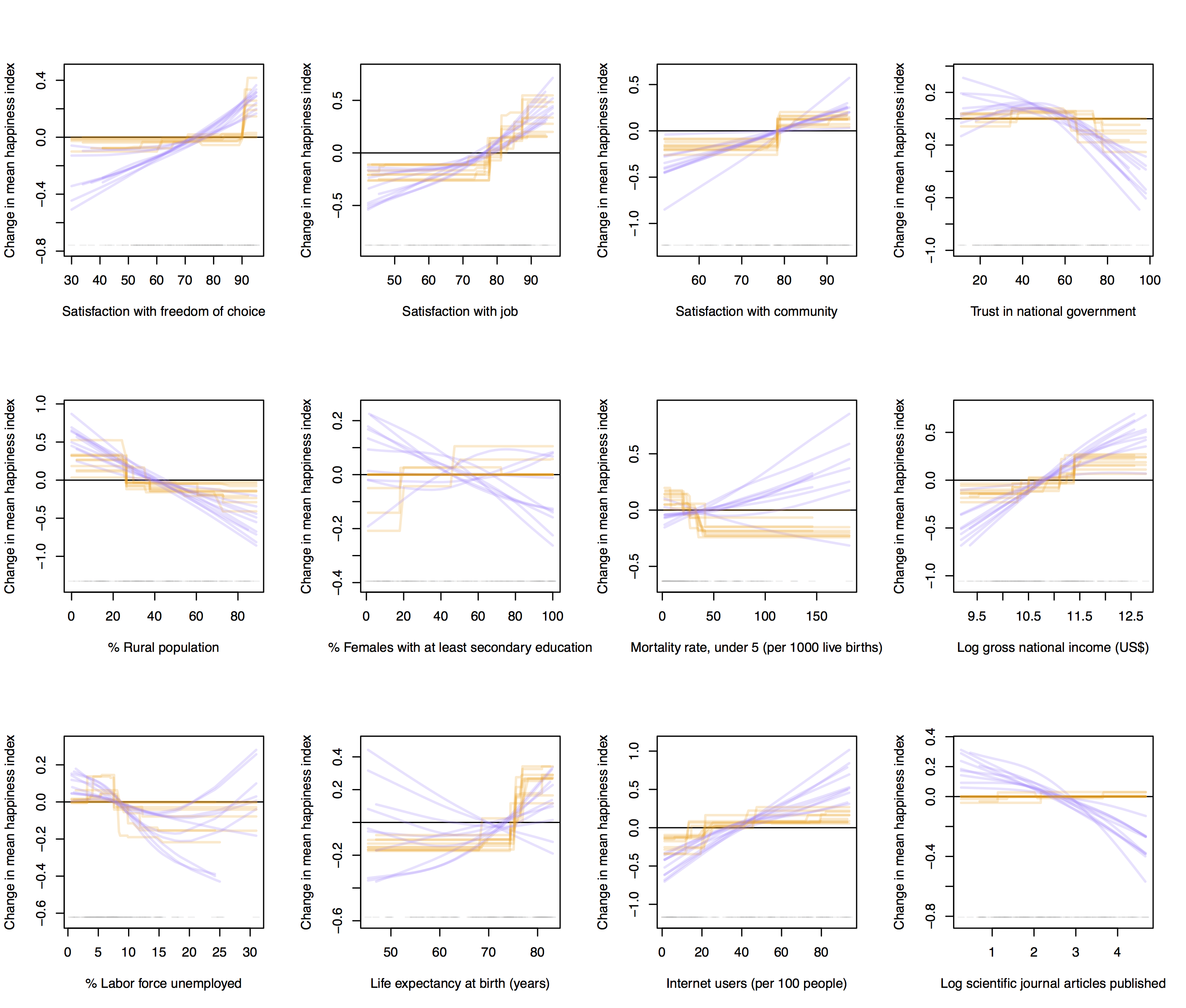
Figure 5: Conditional associations between the happiness index for a country and twelve country-level predictors were estimated using FLAM () and GAM (). Ten fits for each method were obtained by repeatedly splitting the data into training and test sets. The gray bar at the bottom of each plot indicates the distribution of that predictor.

6.2 Classification based on Gene Expression

In this section, we apply FLAM with logistic loss (to be discussed in Section 7), in order to perform classification using gene expression measurements. The data sets we consider are:

1. Autism (Alter et al., 2011): 1498 gene expression measurements from peripheral blood lymphocytes sampled from 82 children with autism and 60 controls, publicly available from GEO at accession number GDS4431 (Barrett et al., 2007).

2. Lung S (Spira et al., 2007): 22,283 gene expression measurements from large airway epithelial cells sampled from 97 smokers with lung cancer and 90 smokers without lung cancer, available from GEO at accession number GDS2771.

3. Lung NS (Lu et al., 2010): 54,675 gene expression measurements from 60 pairs of tumor and adjacent normal lung tissue from non-smoking women with non-small cell lung carcinoma, available from GEO at accession number GDS3837.

We consider only the 2000 genes with the largest variance in the Lung S and Lung NS data sets. We compare the performances of FLAM to SpAM and $\ell_{1}$-penalized logistic regression over 30 splits of the data into training and test sets, after standardizing each gene to have mean zero and variance one in the training set. We choose the tuning parameters using 10-fold CV in the training set and calculate the misclassification rate in the test set.

Test error and sparsity (the percent of genes not used in the classifier) are shown in Figure 6. FLAM has the same or better predictive performance on average as SpAM, but uses a less sparse classifier. However, lasso’s performance is comparable to FLAM and SpAM, which indicates that the sample size may be too small to successfully model non-linear relationships in these three data sets.

For one split of the Lung S data, Figure 6 displays the estimated fits from FLAM, SpAM, and lasso for six genes. These six genes were selected because they were among the 15 with the highest-variance fits for both FLAM and SpAM. Note that the since the genes estimated to have a non-zero relationship with the response differed for each method, the conditional fits shown for a particular gene are not directly comparable across methods.

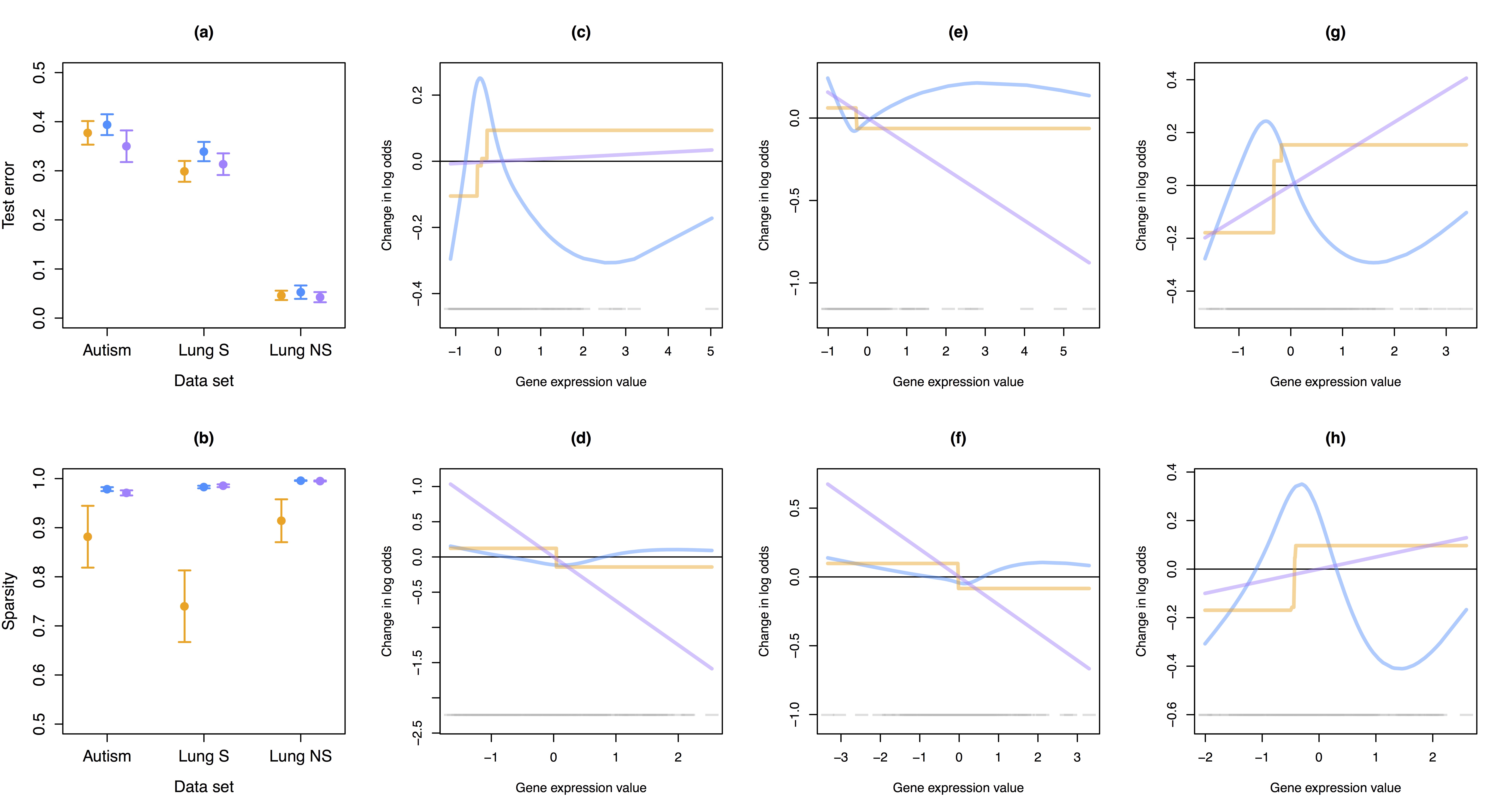
Figure 6: We compare the classification performance of FLAM () to SpAM () and lasso () in terms of (a) test set error and (b) sparsity for three gene expression data sets. Both plots show mean estimates with 95% confidence intervals, which are calculated using 30 splits of the data into training and test sets. In (c)-(h), for six genes we show the fits from FLAM (), SpAM (), and lasso (), which were estimated from one split of the Lung S data. The gray bar at the bottom of each plot indicates the distribution of that predictor.

7 Extensions to FLAM

We now consider the general optimization problem

$$\underset{{\bm{\theta}}\in\mathbb{R}^{np}}{\mathrm{minimize}}\quad\ell({\bm{\theta}})+\lambda\sum_{j=1}^{p}Q_{j}({\bm{\theta}}_{j}),$$ (15)

where ${\bm{\theta}}=({\bm{\theta}}_{1}^{T}\;\cdots\;{\bm{\theta}}_{p}^{T})^{T}$, $\ell:\mathbb{R}^{np}\to\mathbb{R}$ is a differentiable, convex loss function with Lipschitz continuous gradient, and $Q_{j}(\cdot)$ is a convex penalty function. Thus far we have considered (15) for squared error loss, i.e., $\ell({\bm{\theta}})=\frac{1}{2}\left\|{\bm{y}}-\sum_{j=1}^{p}{\bm{\theta}}_{j}-\theta_{0}{\bm{1}}\right\|_{2}^{2}$, and $Q_{j}({\bm{\theta}}_{j})=\alpha\left\|{\bm{D}}{\bm{P}}_{j}{\bm{\theta}}_{j}\right\|_{1}+(1-\alpha)\left\|{\bm{\theta}}_{j}\right\|_{2}$ for $\alpha\in[0,1]$. In this section, we discuss extensions of FLAM to (1) other losses $\ell({\bm{\theta}})$ and (2) other penalties $Q_{j}$.

7.1 A General Algorithm

Generalized gradient descent (GGD) can be used to solve (15) (Beck and Teboulle, 2009). That is, (15) can be solved by choosing an initial $\hat{\bm{\theta}}^{0}$ and continually updating

$$\hat{\bm{\theta}}^{k}=\displaystyle\underset{{\bm{\theta}}\in\mathbb{R}^{np}}{\mathrm{argmin}}\quad\frac{L}{2}\left\|{\bm{\theta}}-\hat{\bm{\theta}}^{k-1}+\frac{1}{L}\dot{\ell}(\hat{\bm{\theta}}^{k-1})\right\|_{2}^{2}+\lambda\sum_{j=1}^{p}Q_{j}({\bm{\theta}}_{j})$$ (16)

until convergence of the objective of (15), where $L\in\mathbb{R}$ is such that $\ddot{\ell}(\cdot)\preceq L{\bm{I}}$. Equation 16 is separable in ${\bm{\theta}}_{j}$, so the features can be updated in parallel during each iteration of GGD (in contrast to coordinate descent, in which the features are updated sequentially). In the special case of (15) given in (5), GGD provides an alternative to Algorithm 1. Details are omitted in the interest of brevity.

7.2 Generalized FLAM

We now consider the model $\mbox{E}[y_{i}|{\bm{x}}_{i}]=g\left(\sum_{j=1}^{p}f_{j}(x_{ij})\right)$, where $g(\cdot)$ is a specified function. For instance, in the case of a binary response, we can consider the mean model $\mbox{E}[y_{i}|{\bm{x}}_{i}]=\text{expit}(\theta_{0}+\sum_{j=1}^{p}\theta_{ji})$, define ${\bm{\theta}}=(\theta_{0}{\bm{1}}^{T}\;{\bm{\theta}}_{1}^{T}\;\cdots\;{\bm{\theta}}_{p}^{T})^{T}$, and take the loss to be logistic,

$$\ell({\bm{\theta}})=-{\bm{y}}^{T}\left(({\bm{1}}_{p+1}^{T}\otimes{\bm{I}}_{n}){\bm{\theta}}\right)+{\bm{1}}^{T}\log\left(1+\exp\left(({\bm{1}}_{p+1}^{T}\otimes{\bm{I}}_{n}){\bm{\theta}}\right)\right).$$

We then solve (15) by continually updating (16), which amounts to the updates

$$\hat{\theta}_{0}^{k}=\hat{\theta}_{0}^{k-1}-\frac{4}{n(p+1)}\left[\text{expit}\left(\hat{\theta}_{0}^{k-1}{\bm{1}}+\sum_{j=1}^{p}\hat{\bm{\theta}}^{k-1}_{j}\right)-{\bm{y}}\right]^{T}{\bm{1}}$$

$$\hat{\bm{\theta}}_{j}^{k}=\underset{{\bm{\theta}}_{j}\in\mathbb{R}^{n}}{\mathrm{argmin}}\quad\frac{p+1}{8}\left\|{\bm{\theta}}_{j}-\hat{\bm{\theta}}^{k-1}_{j}+\frac{4}{p+1}\left[\text{expit}\left(\hat{\theta}_{0}^{k-1}{\bm{1}}+\sum_{j=1}^{p}\hat{\bm{\theta}}^{k-1}_{j}\right)-{\bm{y}}\right]\right\|_{2}^{2}+\lambda Q_{j}({\bm{\theta}}_{j})$$ (17)

for $j=1,\ldots,p$. The solution of (17) follows from Corollary 3.1 when $Q_{j}({\bm{\theta}}_{j})=\alpha\left\|{\bm{D}}{\bm{P}}_{j}{\bm{\theta}}_{j}\right\|_{1}+(1-\alpha)\left\|{\bm{\theta}}_{j}\right\|_{2}$ for $\alpha\in[0,1]$. We now consider (17) with a more general form of $Q_{j}$.

7.3 FLAM with an Alternative Penalty

Thus far, we have seen that (15) can be solved by repeatedly solving a problem of the form (16). When $Q_{j}({\bm{\theta}}_{j})=\alpha\left\|{\bm{D}}{\bm{P}}_{j}{\bm{\theta}}_{j}\right\|_{1}+(1-\alpha)\left\|{\bm{\theta}}_{j}\right\|_{2}$ for $\alpha\in[0,1]$, the solution to (16) follows from Corollary 3.1. Lemma 7.1 generalizes this Corollary to other forms of the penalty $Q_{j}$.

Lemma 7.1

For any norm $\|\cdot\|$, and any matrix ${\bm{B}}$ with $n$ columns, the solution to

$$\underset{{\bm{\theta}}\in\mathbb{R}^{n}}{\mathrm{minimize}}\quad\frac{1}{2}\left\|{\bm{y}}-{\bm{\theta}}\right\|_{2}^{2}+\alpha\lambda\left\|{\bm{B}}{\bm{\theta}}\right\|+(1-\alpha)\lambda\left\|{\bm{\theta}}\right\|_{2}$$ (18)

is $\left(1-\frac{(1-\alpha)\lambda}{\left\|\hat{\bm{\theta}}\right\|_{2}}\right)_{+}\hat{\bm{\theta}}$,  where $(u)_{+}=\max(u,0)$ and $\hat{\bm{\theta}}$ is the solution to

$$\underset{{\bm{\theta}}\in\mathbb{R}^{n}}{\mathrm{minimize}}\quad\frac{1}{2}\left\|{\bm{y}}-{\bm{\theta}}\right\|_{2}^{2}+\alpha\lambda\left\|{\bm{B}}{\bm{\theta}}\right\|.$$ (19)

7.4 Simulations for Generalized FLAM using Logistic Loss

We now present simulation results of FLAM for logistic loss and $Q_{j}({\bm{\theta}}_{j})=\lambda\left\|{\bm{D}}{\bm{P}}_{j}{\bm{\theta}}_{j}\right\|_{1}$. Data are generated according to $y_{i}\stackrel{{\scriptstyle iid}}{{\sim}}\text{Bernoulli}(\text{expit}[f_{1}(x_{i1})+f_{2}(x_{i2})])$ with $x_{ij}\stackrel{{\scriptstyle iid}}{{\sim}}\text{Uniform}[-2.5,2.5],$ where $f_{1}$ and $f_{2}$ are taken to be two of the piecewise constant functions considered previously (Figure 2(a)). Figure 7(a) shows the expectation of $y_{i}$ as a function of $x_{1}$ and $x_{2}$. For each replication, we generate training and test sets with $n=100$. We choose the value $\lambda$ corresponding to the minimum test set MSE. The estimated expectation of $y_{i}$ averaged over 25 data replicates is displayed in Figure 7(b). It closely mirrors Figure 7(a).

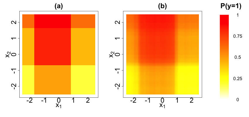
Figure 7: We compare (a) the true expectation of $y_{i}$ to (b) the estimated expectation of $y_{i}$ (averaged over 25 data replicates) obtained from FLAM with logistic loss for combinations of the two predictors, $x_{1}$ and $x_{2}$.

8 Discussion

We have presented the fused lasso additive model, a flexible yet interpretable framework for prediction, for which the estimated fits are piecewise constant with data-adaptive knots.

While the $\ell_{1}$ penalty in (5) limits the number of knots in the fits, it also shrinks the magnitude of jumps where knots do occur. However, the resulting shrinkage can easily be addressed by debiasing the fit. That is, FLAM can be used to identify the knots; then the piecewise constant model can be refit using standard linear regression with the appropriate basis functions for the known knots.

While the piecewise constant framework has much flexibility, a large number of knots are needed to accommodate trends with large slopes. Piecewise linear fits are more suited to this type of relationship. The problem of estimating piecewise trends of any order between a single predictor and response has been previously explored (Kim et al., 2009; Tibshirani, 2014). We leave the extension of FLAM to this setting to future work.

The R package FLAM will be made available on CRAN. The R package Shiny (RStudio and Inc., 2014) was used to develop interactive web applications demonstrating the performance of FLAM on simulated and user-uploaded data (students.washington.edu/ajpete).

Appendix A Appendix

A.1 Proof of Lemma 4.1

Differentiating (5) with respect to $\theta_{0}$ gives $\hat{\theta}_{0}=\frac{1}{n}{\bm{1}}^{T}\left({\bm{y}}-\sum_{j=1}^{p}{\bm{\theta}}_{j}\right)=\frac{1}{n}{\bm{1}}^{T}{\bm{y}}$, since ${\bm{1}}^{T}{\bm{\theta}}_{j}=0$ for $j=1,\ldots,p$. Thus we can solve (5) with ${\bm{y}}$ centered and no intercept. We now reparameterize in terms of ${\bm{\beta}}_{j}\in\mathbb{R}^{n-1}$ where ${\bm{\beta}}_{j}={\bm{D}}{\bm{P}}_{j}{\bm{\theta}}_{j}$. Note that

$${\bm{\theta}}_{j}={\bm{P}}_{j}^{T}{\bm{P}}_{j}{\bm{\theta}}_{j}={\bm{P}}_{j}^{T}\left({\bm{U}}{\bm{D}}+\frac{1}{n}{\bm{1}}{\bm{1}}^{T}\right){\bm{P}}_{j}{\bm{\theta}}_{j}={\bm{P}}_{j}^{T}{\bm{U}}{\bm{\beta}}_{j},$$

using the facts that ${\bm{U}}{\bm{D}}+\frac{1}{n}{\bm{1}}{\bm{1}}^{T}={\bm{I}}$ and ${\bm{1}}^{T}{\bm{P}}_{j}{\bm{\theta}}_{j}=0$. Defining ${\bm{\beta}}=({\bm{\beta}}_{1}^{T}\;\cdots\;{\bm{\beta}}_{p}^{T})^{T}\in\mathbb{R}^{(n-1)p}$ and ${\bm{V}}=[{\bm{P}}_{1}^{T}{\bm{U}}\cdots{\bm{P}}_{p}^{T}{\bm{U}}]$, we see that (5) can be rewritten as (8).

A.2 Proof of Proposition 4.2

We first derive the degrees of freedom for $\hat{\bm{y}}$ for (10) when ${\bm{y}}\sim MVN({\bm{0}},\sigma^{2}{\bm{I}})$. Using the dual problem of (10) and Lemma 1 of Tibshirani et al. [2012], it can be shown that $g:\mathbb{R}^{n}\to\mathbb{R}^{n}$ with $\hat{\bm{y}}=g({\bm{y}})=\left(g_{1}({\bm{y}}),\ldots,g_{n}({\bm{y}})\right)^{T}$ is continuous and almost differentiable. Thus, Stein’s lemma implies that $\text{df}(\hat{\bm{y}})=\mbox{E}\left[\mbox{Tr}\left(\frac{\partial g({\bm{y}})}{\partial{\bm{y}}}\right)\right]$. We denote the active set of $\hat{\bm{\beta}}$ as $\mathcal{A}$, which is unique since (10) is strictly convex. At the optimum of (10), we have

$${\bm{0}}=-{\bm{V}}_{\mathcal{A}}^{T}\left({\bm{y}}-{\bm{V}}_{\mathcal{A}}\hat{\bm{\beta}}_{\mathcal{A}}\right)+\alpha\lambda\text{sign}\left(\hat{\bm{\beta}}_{\mathcal{A}}\right)+(1-\alpha)\lambda S_{1}+\epsilon\hat{\bm{\beta}}_{\mathcal{A}},$$ (20)

where $S_{1}=\frac{\partial}{\partial\hat{\bm{\beta}}_{\mathcal{A}}}\sum_{j=1}^{p}\left\|{\bm{U}}{\bm{\beta}}_{j}\right\|_{2}=\left[S_{1,1}^{T}\cdots S_{1,p}^{T}\right]^{T}$ with $S_{1,j}=\frac{{\bm{U}}_{\mathcal{A}_{j}}^{T}{\bm{U}}_{\mathcal{A}_{j}}\hat{\bm{\beta}}_{j\mathcal{A}_{j}}}{\|{\bm{U}}_{\mathcal{A}_{j}}\hat{\bm{\beta}}_{j\mathcal{A}_{j}}\|_{2}}.$

We conjecture that there is a neighborhood around almost every ${\bm{y}}$ (i.e., except a set of measure zero) such that $\hat{\bm{\beta}}^{*}$ corresponding to any ${\bm{y}}^{*}$ in that neighborhood has $\mathcal{A}^{*}=\mathcal{A}$ and $\text{sign}(\hat{\bm{\beta}}^{*}_{\mathcal{A}^{*}})=\text{sign}(\hat{\bm{\beta}}_{\mathcal{A}})$. On the basis of this conjecture, we treat $\mathcal{A}$ and $\text{sign}(\hat{\bm{\beta}}_{\mathcal{A}})$ in (20) as constants with respect to ${\bm{y}}$. Thus the derivative of (20) with respect to ${\bm{y}}$ is

$${\bm{0}}=-{\bm{V}}_{\mathcal{A}}^{T}+{\bm{V}}_{\mathcal{A}}^{T}{\bm{V}}_{\mathcal{A}}\frac{\partial\hat{\bm{\beta}}_{\mathcal{A}}}{\partial{\bm{y}}}+(1-\alpha)\lambda S_{2}\frac{\partial\hat{\bm{\beta}}_{\mathcal{A}}}{\partial{\bm{y}}}+\epsilon\frac{\partial\hat{\bm{\beta}}_{\mathcal{A}}}{\partial{\bm{y}}},$$ (21)

where $S_{2}=\frac{\partial S_{1}}{\partial\hat{\bm{\beta}}_{\mathcal{A}}}$ is a block diagonal matrix with the $j$th block equaling

$$\frac{{\bm{U}}_{\mathcal{A}_{j}}^{T}{\bm{U}}_{\mathcal{A}_{j}}}{\|{\bm{U}}_{\mathcal{A}_{j}}\hat{\bm{\beta}}_{j\mathcal{A}_{j}}\|_{2}}-\frac{{\bm{U}}_{\mathcal{A}_{j}}^{T}{\bm{U}}_{\mathcal{A}_{j}}\hat{\bm{\beta}}_{j\mathcal{A}_{j}}\hat{\bm{\beta}}_{j\mathcal{A}_{j}}^{T}{\bm{U}}_{\mathcal{A}_{j}}^{T}{\bm{U}}_{\mathcal{A}_{j}}}{\|{\bm{U}}_{\mathcal{A}_{j}}\hat{\bm{\beta}}_{j\mathcal{A}_{j}}\|_{2}^{3}}.$$

Solving (21) for $\frac{\partial\hat{\bm{\beta}}_{\mathcal{A}}}{\partial{\bm{y}}}$ and left multiplying by ${\bm{V}}_{\mathcal{A}}$, we have

$$\frac{\partial\hat{\bm{y}}}{\partial{\bm{y}}}={\bm{V}}_{\mathcal{A}}\frac{\partial\hat{\bm{\beta}}_{\mathcal{A}}}{\partial{\bm{y}}}={\bm{V}}_{\mathcal{A}}\left[{\bm{V}}_{\mathcal{A}}^{T}{\bm{V}}_{\mathcal{A}}+(1-\alpha)\lambda S_{2}+\epsilon{\bm{I}}\right]^{-1}{\bm{V}}_{\mathcal{A}}^{T}.$$

Therefore, the degrees of freedom are $\mbox{E}\left[\mbox{Tr}\left({\bm{V}}_{\mathcal{A}}\left[{\bm{V}}_{\mathcal{A}}^{T}{\bm{V}}_{\mathcal{A}}+(1-\alpha)\lambda S_{2}+\epsilon{\bm{I}}\right]^{-1}{\bm{V}}_{\mathcal{A}}^{T}\right)\right].$ This yields the estimator (11), where one degree of freedom is added for the intercept.

The proof of Proposition 4.4 is omitted, as it follows the arguments in this proof closely.

A.3 Proof of Lemma 4.5

The optimality condition for (8) with $\alpha=1$ is $-{\bm{V}}^{T}(\tilde{\bm{y}}-{\bm{V}}{\bm{\beta}})+\lambda s({\bm{\beta}})=0$, where $s({\bm{\beta}}_{j})=\text{sign}({\bm{\beta}}_{j})$ if ${\bm{\beta}}_{j}\neq 0$ and $s({\bm{\beta}}_{j})\in[-1,1]$ if ${\bm{\beta}}_{j}=0$. After plugging in ${\bm{\beta}}={\bm{0}}$, we obtain $-{\bm{V}}^{T}\tilde{\bm{y}}+\lambda s({\bm{0}})={\bm{0}}$, which is satisfied if and only if $\lambda\geq\|{\bm{V}}^{T}\tilde{\bm{y}}\|_{\infty}$ since $s({\bm{0}})\in[-1,1]$.

Now we consider the optimality condition for (5) when $\alpha=0$, which takes the form $-\tilde{\bm{y}}+\sum_{j=1}^{p}{\bm{\theta}}_{j}+\lambda s({\bm{\theta}}_{j})={\bm{0}}$ for $j=1,\ldots,p,$ where $s({\bm{\theta}}_{j})={\bm{\theta}}_{j}/\|{\bm{\theta}}_{j}\|_{2}$ if ${\bm{\theta}}_{j}\neq{\bm{0}}$ and $s({\bm{\theta}}_{j})\in\{{\bm{g}}\mid\|{\bm{g}}\|_{2}\leq 1\}$ if ${\bm{\theta}}_{j}={\bm{0}}$. After plugging in ${\bm{\theta}}_{j}={\bm{0}}$ for $j=1,\ldots,p$, we obtain $-\tilde{\bm{y}}+\lambda s({\bm{0}})={\bm{0}}$, which is satisfied if and only if $\lambda\geq\|\tilde{\bm{y}}\|_{2}$.

A.4 Proof of Corollary 4.6

The objective of (5) is bounded below by

$$\underset{\theta_{0}\in\mathbb{R},{\bm{\theta}}_{j}\in\mathbb{R}^{n},1\leq j\leq p}{\mathrm{min}}\quad\frac{1}{2}\left\|{\bm{y}}-\sum_{j=1}^{p}{\bm{\theta}}_{j}-\theta_{0}\bf{1}\right\|_{2}^{2}+\alpha\lambda\sum_{j=1}^{p}\left\|{\bm{D}}{\bm{P}}_{j}{\bm{\theta}}_{j}\right\|_{1}$$ (22)

and

$$\underset{\theta_{0}\in\mathbb{R},{\bm{\theta}}_{j}\in\mathbb{R}^{n},1\leq j\leq p}{\mathrm{min}}\quad\frac{1}{2}\left\|{\bm{y}}-\sum_{j=1}^{p}{\bm{\theta}}_{j}-\theta_{0}\bf{1}\right\|_{2}^{2}+(1-\alpha)\lambda\sum_{j=1}^{p}\left\|{\bm{\theta}}_{j}\right\|_{2}$$ (23)

for any $\alpha\in[0,1]$ and $\lambda\geq 0$. Lemma 4.5 implies that if $\lambda\geq\min\left(\frac{\|{\bm{V}}^{T}\tilde{\bm{y}}\|_{\infty}}{\alpha},\frac{\|\tilde{\bm{y}}\|_{2}}{1-\alpha}\right),$ then the objective of (5) is bounded below by $\underset{\theta_{0}\in\mathbb{R}}{\mathrm{min}}\quad\frac{1}{2}\left\|{\bm{y}}-\theta_{0}\bf{1}\right\|_{2}^{2}=\frac{1}{2}\left\|{\bm{y}}-\frac{1}{n}{\bm{1}}^{T}{\bm{y}}\bf{1}\right\|_{2}^{2}$. The objective of (5) achieves this lower bound when $\hat{\bm{\theta}}_{j}={\bm{0}}$ for $j=1,\ldots,p$.

A.5 Proof of Lemma 4.7

Fact A.1

Let ${\bm{z}}_{j}\in\mathbb{R}^{n}\sim MVN({\bm{0}},\Sigma)$ with $\underset{1\leq i\leq n}{\max}\Sigma_{i,i}\leq c$ for $j=1,\ldots,p$. Then

$$P\left(\underset{1\leq j\leq p}{\max}\|{\bm{z}}_{j}\|_{\infty}\geq 2\sqrt{c\log(np)}\right)\leq\frac{2}{np}.$$

Proof: Note that $P(z_{ji}\geq 2\sqrt{c\log(np)})\leq P(z_{0}\geq 2\sqrt{c\log(np)})$ where $z_{0}\sim N(0,c)$. Thus

$$P\left(\underset{1\leq j\leq p}{\max}\|{\bm{z}}_{j}\|_{\infty}\geq 2\sqrt{c\log(np)}\right)\leq 2npP\left(z_{0}/\sqrt{c}\geq 2\sqrt{\log(np)}\right)\leq\frac{2}{np},$$

which follows from the union bound and the fact that

$$P\left(z_{0}/\sqrt{c}\geq 2\sqrt{\log(np)}\right)=\int_{2\sqrt{\log(np)}}^{\infty}\frac{1}{\sqrt{2\pi}}\exp\left(\frac{-t^{2}}{2}\right)dt\leq\int_{2\sqrt{\log(np)}}^{\infty}t\exp\left(\frac{-t^{2}}{2}\right)dt=\frac{1}{n^{2}p^{2}}.$$

Fact A.2

Let ${\bm{z}}\in\mathbb{R}^{n}\sim MVN({\bm{0}},c{\bm{I}})$. Then $P\left(\|{\bm{z}}\|_{2}\geq\sqrt{cn\left(1+\sqrt{\frac{4\log n}{n}}+\frac{4\log n}{n}\right)}\right)\leq\frac{1}{n}.$

Proof: Since $\|{\bm{z}}\|_{2}^{2}\sim c\chi_{n}^{2}$, this follows from Lemma 8.1 in Bühlmann and Van De Geer [2011].

We now establish prediction consistency. We rewrite (5) as

$$\underset{{\bm{\theta}}\in\mathbb{R}^{np}}{\mathrm{minimize}}\quad\frac{1}{2n}\left\|{\bm{y}}-{\bm{W}}{\bm{\theta}}\right\|_{2}^{2}+\lambda\Omega({\bm{\theta}}),$$

where ${\bm{W}}={\bm{1}}^{T}\otimes{\bm{I}}_{n}$ and $\Omega({\bm{\theta}})=\sum_{j=1}^{p}\left[\alpha\left\|{\bm{D}}{\bm{P}}_{j}{\bm{\theta}}_{j}\right\|_{1}+(1-\alpha)\|{\bm{\theta}}_{j}\|_{2}\right]$. Denote the true coefficient vector as ${\bm{\theta}}^{0}=({\bm{\theta}}_{1}^{0T}\cdots{\bm{\theta}}_{p}^{0T})^{T}$ and assume ${\bm{y}}={\bm{W}}{\bm{\theta}}^{0}+{\bm{\epsilon}}$ with ${\bm{\epsilon}}\sim MVN({\bm{0}},\sigma^{2}{\bm{I}})$. By the definition of $\hat{\bm{\theta}}$, $\frac{1}{2n}\left\|{\bm{y}}-{\bm{W}}\hat{\bm{\theta}}\right\|_{2}^{2}+\lambda\Omega(\hat{\bm{\theta}})\leq\frac{1}{2n}\left\|{\bm{y}}-{\bm{W}}{\bm{\theta}}^{0}\right\|_{2}^{2}+\lambda\Omega({\bm{\theta}}^{0}),$ so

$$\frac{1}{2n}\left\|\sum_{j=1}^{p}(\hat{\bm{\theta}}_{j}-{\bm{\theta}}_{j}^{0})\right\|_{2}^{2}+\lambda\Omega(\hat{\bm{\theta}})\leq V_{n}(\hat{\bm{\theta}})+\lambda\Omega({\bm{\theta}}^{0})$$ (24)

where $V_{n}(\hat{\bm{\theta}})=\frac{1}{n}\sum_{j=1}^{p}{\bm{\epsilon}}^{T}(\hat{\bm{\theta}}_{j}-{\bm{\theta}}_{j}^{0}).$ We wish to bound the empirical process $V_{n}(\hat{\bm{\theta}})$. We have

$$\left|V_{n}(\hat{\bm{\theta}})\right| =\frac{1}{\sqrt{n}}\left|\sum_{j=1}^{p}\left[\frac{\alpha}{\sqrt{n}}{\bm{\epsilon}}^{T}{\bm{P}}_{j}^{T}{\bm{U}}{\bm{D}}{\bm{P}}_{j}(\hat{\bm{\theta}}_{j}-{\bm{\theta}}_{j}^{0})+\frac{1-\alpha}{\sqrt{n}}{\bm{\epsilon}}^{T}(\hat{\bm{\theta}}_{j}-{\bm{\theta}}_{j}^{0})\right]\right|$$

$$\leq\frac{1}{\sqrt{n}}\sum_{j=1}^{p}\left[\left|\frac{\alpha}{\sqrt{n}}{\bm{\epsilon}}^{T}{\bm{P}}_{j}^{T}{\bm{U}}{\bm{D}}{\bm{P}}_{j}(\hat{\bm{\theta}}_{j}-{\bm{\theta}}_{j}^{0})\right|+\left|\frac{1-\alpha}{\sqrt{n}}{\bm{\epsilon}}^{T}(\hat{\bm{\theta}}_{j}-{\bm{\theta}}_{j}^{0})\right|\right]$$

$$\leq\frac{1}{\sqrt{n}}\sum_{j=1}^{p}\left[\|{\bm{v}}_{1j}\|_{\infty}\alpha\|{\bm{D}}{\bm{P}}_{j}(\hat{\bm{\theta}}_{j}-{\bm{\theta}}_{j}^{0})\|_{1}+\|{\bm{v}}_{2}\|_{2}(1-\alpha)\|\hat{\bm{\theta}}_{j}-{\bm{\theta}}_{j}^{0}\|_{2}\right]$$

$$\leq\frac{\underset{1\leq j\leq p}{\max}\|{\bm{v}}_{1j}\|_{\infty}}{\sqrt{n}}\sum_{j=1}^{p}\alpha\left(\|{\bm{D}}{\bm{P}}_{j}\hat{\bm{\theta}}_{j}\|_{1}+\|{\bm{D}}{\bm{P}}_{j}{\bm{\theta}}_{j}^{0}\|_{1}\right)+\frac{\|{\bm{v}}_{2}\|_{2}}{\sqrt{n}}\sum_{j=1}^{p}(1-\alpha)\left(\|\hat{\bm{\theta}}_{j}\|_{2}+\|{\bm{\theta}}_{j}^{0}\|_{2}\right)$$

where ${\bm{v}}_{1j}=\frac{1}{\sqrt{n}}{\bm{U}}^{T}{\bm{P}}_{j}{\bm{\epsilon}}$ and ${\bm{v}}_{2}=\frac{1}{\sqrt{n}}{\bm{\epsilon}}$.

We now establish bounds for $\underset{1\leq j\leq p}{\max}\|{\bm{v}}_{1j}\|_{\infty}$ and $\|{\bm{v}}_{2}\|_{2}$ that hold with large probability.

Note that ${\bm{v}}_{1j}\in\mathbb{R}^{n-1}\sim MVN({\bm{0}},\frac{\sigma^{2}}{n}{\bm{U}}^{T}{\bm{U}})$. Since $\underset{1\leq i\leq n}{\max}(\frac{\sigma^{2}}{n}{\bm{U}}^{T}{\bm{U}})_{i,i}\leq\frac{\sigma^{2}}{4}$, Fact A.1 with $c=\frac{\sigma^{2}}{4}$ gives $P\left(\underset{1\leq j\leq p}{\max}\frac{\|{\bm{v}}_{1j}\|_{\infty}}{\sqrt{n}}\geq w_{1}\right)\leq\frac{2}{(n-1)p}$ where $w_{1}=\sigma\sqrt{\frac{\log((n-1)p)}{n}}$. Now recall ${\bm{v}}_{2}\sim MVN({\bm{0}},\frac{\sigma^{2}}{n}{\bm{I}})$, so by Fact A.2, $P\left(\frac{\|{\bm{v}}_{2}\|_{2}}{\sqrt{n}}\geq w_{2}\right)\leq\frac{1}{n}$ where $w_{2}=\frac{\sigma}{\sqrt{n}}\sqrt{1+\sqrt{\frac{4\log n}{n}}+\frac{4\log n}{n}}$.

Therefore, with probability at least $1-\left(\frac{2}{(n-1)p}+\frac{1}{n}\right)$,

$$|V_{n}(\hat{\bm{\theta}})|\leq\sum_{j=1}^{p}[w_{1}\alpha(\|{\bm{D}}{\bm{P}}_{j}\hat{\bm{\theta}}_{j}\|_{1}+\|{\bm{D}}{\bm{P}}_{j}{\bm{\theta}}_{j}^{0}\|_{1})+w_{2}(1-\alpha)(\|\hat{\bm{\theta}}_{j}\|_{2}+\|{\bm{\theta}}_{j}^{0}\|_{2})].$$

Let $\lambda=2w_{1}$. For $p\geq 1$ and $n\geq 15$, $w_{1}>w_{2}$. Thus, with high probability,

$$|V_{n}(\hat{\bm{\theta}})|\leq\frac{\lambda}{2}\sum_{j=1}^{p}[\alpha(\|{\bm{D}}{\bm{P}}_{j}\hat{\bm{\theta}}_{j}\|_{1}+\|{\bm{D}}{\bm{P}}_{j}{\bm{\theta}}_{j}^{0}\|_{1})+(1-\alpha)(\|\hat{\bm{\theta}}_{j}\|_{2}+\|{\bm{\theta}}_{j}^{0}\|_{2})]=\frac{\lambda}{2}(\Omega(\hat{\bm{\theta}})+\Omega({\bm{\theta}}^{0})).$$ (25)

The result follows from plugging the bound from (25) into (24).

A.6 Derivations of Results from Section 7.2

For $\ell({\bm{\theta}})$ of the form (7.2), we can calculate

$$\dot{\ell}({\bm{\theta}}) = ({\bm{1}}_{p+1}\otimes{\bm{I}}_{n})\left[\text{expit}(({\bm{1}}_{p+1}^{T}\otimes{\bm{I}}_{n}){\bm{\theta}})-{\bm{y}}\right]$$

$$\ddot{\ell}({\bm{\theta}}) = ({\bm{1}}_{p+1}\otimes{\bm{I}}_{n})\text{diag}\left(\text{expit}(({\bm{1}}_{p+1}^{T}\otimes{\bm{I}}_{n}){\bm{\theta}})(1-\text{expit}(({\bm{1}}_{p+1}^{T}\otimes{\bm{I}}_{n}){\bm{\theta}}))\right)({\bm{1}}_{p+1}^{T}\otimes{\bm{I}}_{n})$$

$$\preceq \frac{1}{4}({\bm{1}}_{p+1}{\bm{1}}_{p+1}^{T}\otimes{\bm{I}}_{n})\preceq\frac{1}{4}(p+1){\bm{I}}.$$

Thus, plugging in $L=\frac{1}{4}(p+1)$ and $\dot{\ell}({\bm{\theta}})$ into (16), we now have

$$\hat{\bm{\theta}}^{k}=\displaystyle\underset{{\bm{\theta}}\in\mathbb{R}^{n(p+1)}}{\mathrm{argmin}}\quad\displaystyle\frac{p+1}{8}\left\|{\bm{\theta}}-\hat{\bm{\theta}}^{k-1}+\frac{4}{p+1}({\bm{1}}_{p+1}\otimes{\bm{I}}_{n})\left[\text{expit}(({\bm{1}}_{p+1}^{T}\otimes{\bm{I}}_{n})\hat{\bm{\theta}}^{k-1})-{\bm{y}}\right]\right\|_{2}^{2}+\lambda\sum_{j=1}^{p}Q_{j}({\bm{\theta}}_{j}).$$

This is separable in ${\bm{\theta}}_{j}$, and is equivalent to (17) by inspection.

A.7 Proof of Lemma 7.1

There are two main tasks:

• Task 1: Derive the form of $\hat{\bm{\theta}}$, the solution to (19).

• Task 2: Show that the solution to (18) is $\tilde{\bm{\theta}}=(1-(1-\alpha)\lambda/\|\hat{\bm{\theta}}\|_{2})_{+}\hat{\bm{\theta}}$.

We begin with Task 1. We rewrite (19) as

$$\underset{{\bm{\theta}},{\bm{z}}}{\mathrm{minimize}}\quad\frac{1}{2}\left\|{\bm{y}}-{\bm{\theta}}\right\|_{2}^{2}+\alpha\lambda\left\|{\bm{z}}\right\|\text{ subject to }{\bm{z}}={\bm{B}}{\bm{\theta}},$$

which has Lagrangian $\mathcal{L}({\bm{\theta}},{\bm{z}},{\bm{v}})=\frac{1}{2}\left\|{\bm{y}}-{\bm{\theta}}\right\|_{2}^{2}+\alpha\lambda\left\|{\bm{z}}\right\|+{\bm{v}}^{T}({\bm{B}}{\bm{\theta}}-{\bm{z}}).$ The dual function is

$$g({\bm{v}})=\underset{{\bm{\theta}},{\bm{z}}}{\text{inf}}\enskip\mathcal{L}({\bm{\theta}},{\bm{z}},{\bm{v}})=\underset{{\bm{z}}}{\text{inf}}\left\{\frac{1}{2}\left\|{\bm{B}}^{T}{\bm{v}}\right\|_{2}^{2}+{\bm{v}}^{T}{{\bm{B}}}({\bm{y}}-{\bm{B}}^{T}{\bm{v}})+\alpha\lambda\left\|{\bm{z}}\right\|-{\bm{v}}^{T}{\bm{z}}\right\},$$

where the second equality follows from noting that the partial minimum with respect to ${\bm{\theta}}$ satisfies ${\bm{\theta}}={\bm{y}}-{\bm{B}}^{T}{\bm{v}}$. Thus $g({\bm{v}})=\frac{1}{2}\left\|{\bm{B}}^{T}{\bm{v}}\right\|_{2}^{2}+{\bm{v}}^{T}{{\bm{B}}}({\bm{y}}-{\bm{B}}^{T}{\bm{v}})$ if $\|{\bm{v}}\|_{*}\leq\alpha\lambda$ and $-\infty$ otherwise, where $\|\cdot\|_{*}$ is the dual norm of $\|\cdot\|$. Finally, the dual problem is

$$\underset{\|{\bm{v}}\|_{*}\leq\alpha\lambda}{\mathrm{maximize}}\quad-\frac{1}{2}\left\|{\bm{y}}-{\bm{B}}^{T}{\bm{v}}\right\|_{2}^{2}+\frac{1}{2}{\bm{y}}^{T}{\bm{y}}.$$

Letting $\hat{\bm{v}}=\underset{\|{\bm{v}}\|_{*}\leq\alpha\lambda}{\mathrm{argmin}}\quad\left\|{\bm{y}}-{\bm{B}}^{T}{\bm{v}}\right\|_{2}^{2}$, the solution to (19) is $\hat{\bm{\theta}}={\bm{y}}-{\bm{B}}^{T}\hat{\bm{v}}$.

We now move on to Task 2. Rewriting (18) as

$$\underset{{\bm{\theta}},{\bm{z}}_{1},{\bm{z}}_{2}}{\mathrm{minimize}}\quad\frac{1}{2}\left\|{\bm{y}}-{\bm{\theta}}\right\|_{2}^{2}+\alpha\lambda\left\|{\bm{z}}_{1}\right\|+(1-\alpha)\lambda\left\|{\bm{z}}_{2}\right\|_{2}\text{ subject to }{\bm{z}}_{1}={\bm{B}}{\bm{\theta}},{\bm{z}}_{2}={\bm{\theta}}$$

and writing out the Lagrangian, one can show that the dual problem is

$$\underset{\|{\bm{v}}\|_{*}\leq\alpha\lambda,\|{\bm{u}}\|_{2}\leq(1-\alpha)\lambda}{\mathrm{maximize}}\quad\frac{1}{2}\left\|{\bm{B}}^{T}{\bm{v}}+{\bm{u}}\right\|_{2}^{2}+({\bm{B}}^{T}{\bm{v}}+{\bm{u}})^{T}({\bm{y}}-{\bm{B}}^{T}{\bm{v}}-{\bm{u}});$$ (26)

the calculations to obtain (26) indicate that ${\bm{\theta}}={\bm{y}}-{\bm{B}}^{T}{\bm{v}}-{\bm{u}}$. Problem (26) is equivalent to $\underset{\|{\bm{v}}\|_{*}\leq\alpha\lambda,\|{\bm{u}}\|_{2}\leq(1-\alpha)\lambda}{\mathrm{minimize}}\quad\frac{1}{2}\left\|{\bm{y}}-{\bm{B}}^{T}{\bm{v}}-{\bm{u}}\right\|_{2}^{2}.$ Minimizing in ${\bm{u}}$, we have

$\tilde{\bm{u}}=\begin{cases}{\bm{y}}-{\bm{B}}^{T}{\bm{v}}&\text{if }\left\|{\bm{y}}-{\bm{B}}^{T}{\bm{v}}\right\|_{2}\leq(1-\alpha)\lambda\\ (1-\alpha)\lambda\frac{{\bm{y}}-{\bm{B}}^{T}{\bm{v}}}{\left\|{\bm{y}}-{\bm{B}}^{T}{\bm{v}}\right\|_{2}}&\text{if }\left\|{\bm{y}}-{\bm{B}}^{T}{\bm{v}}\right\|_{2}>(1-\alpha)\lambda\end{cases}$,

the projection of ${\bm{y}}-{\bm{B}}^{T}{\bm{v}}$ onto the $(1-\alpha)\lambda$ ball. Thus (26) is equivalent to

$$\underset{\|{\bm{v}}\|_{*}\leq\alpha\lambda}{\mathrm{minimize}}\quad\left(\left\|{\bm{y}}-{\bm{B}}^{T}{\bm{v}}\right\|_{2}-(1-\alpha)\lambda\right)_{+},$$

which is solved by $\tilde{\bm{v}}=\underset{\|{\bm{v}}\|_{*}\leq\alpha\lambda}{\mathrm{argmin}}\quad\left\|{\bm{y}}-{\bm{B}}^{T}{\bm{v}}\right\|_{2}^{2}$. Therefore, we have shown that $\tilde{\bm{v}}=\hat{\bm{v}}$ and $\tilde{\bm{\theta}}={\bm{y}}-{\bm{B}}^{T}\tilde{\bm{v}}-\tilde{\bm{u}}$. It follows that $\tilde{\bm{\theta}}=\hat{\bm{\theta}}-\tilde{\bm{u}}=\left(1-\frac{(1-\alpha)\lambda}{\|\hat{\bm{\theta}}\|_{2}}\right)_{+}\hat{\bm{\theta}}.$

References

• Alter etย al. (2011) Markย D Alter, Rutwik Kharkar, Keriย E Ramsey, Davidย W Craig, Raunย D Melmed, Theresaย A Grebe, Rย Curtis Bay, Sharman Ober-Reynolds, Janet Kirwan, Joshย J Jones, etย al. Autism and increased paternal age related changes in global levels of gene expression regulation. PloS one, 6(2):e16715, 2011.
• Avalos etย al. (2007) Marta Avalos, Yves Grandvalet, and Christophe Ambroise. Parsimonious additive models. Computational statistics & data analysis, 51(6):2851โ€“2870, 2007.
• Barrett etย al. (2007) Tanya Barrett, Dennisย B Troup, Stephenย E Wilhite, Pierre Ledoux, Dmitry Rudnev, Carlos Evangelista, Ireneย F Kim, Alexandra Soboleva, Maxim Tomashevsky, and Ron Edgar. NCBI GEO: mining tens of millions of expression profiles โ€” database and tools update. Nucleic acids research, 35(suppl 1):D760โ€“D765, 2007.
• Beck and Teboulle (2009) Amir Beck and Marc Teboulle. A fast iterative shrinkage-thresholding algorithm for linear inverse problems. SIAM Journal on Imaging Sciences, 2(1):183โ€“202, 2009.
• Bรผhlmann and Van Deย Geer (2011) Peter Bรผhlmann and Sara Van Deย Geer. Statistics for high-dimensional data: methods, theory and applications. Springer, 2011.
• Cantril (1965) Hadley Cantril. Pattern of human concerns. 1965.
• Efron (1986) Bradley Efron. How biased is the apparent error rate of a prediction rule? Journal of the American Statistical Association, 81(394):461โ€“470, 1986.
• Hastie (2013) Trevor Hastie. gam: Generalized Additive Models, 2013. URL http://CRAN.R-project.org/package=gam. R package version 1.09.
• Hastie and Tibshirani (1986) Trevor Hastie and Robert Tibshirani. Generalized additive models. Statistical science, pages 297โ€“310, 1986.
• Hastie and Tibshirani (1990) Trevorย J Hastie and Robertย J Tibshirani. Generalized additive models, volumeย 43. CRC Press, 1990.
• Helliwell etย al. (2013) Johnย F Helliwell, Richard Layard, Jeffrey Sachs, and Emiratesย Competitiveness Council. World happiness report 2013. Sustainable Development Solutions Network, 2013.
• Hoefling (2010) Holger Hoefling. A path algorithm for the fused lasso signal approximator. Journal of Computational and Graphical Statistics, 19(4):984โ€“1006, 2010.
• Hoefling (2013) Holger Hoefling. flsa: Path algorithm for the general Fused Lasso Signal Approximator, 2013. URL http://CRAN.R-project.org/package=flsa. R package version 1.05.
• Huang etย al. (2010) Jian Huang, Joelย L Horowitz, and Fengrong Wei. Variable selection in nonparametric additive models. Annals of statistics, 38(4):2282, 2010.
• Johnson (2013) Nicholasย A Johnson. A dynamic programming algorithm for the fused lasso and l 0-segmentation. Journal of Computational and Graphical Statistics, 22(2):246โ€“260, 2013.
• Kim etย al. (2009) Seung-Jean Kim, Kwangmoo Koh, Stephen Boyd, and Dimitry Gorinevsky. $\ell_{1}$ trend filtering. SIAM Review, 51(2):339โ€“360, 2009.
• Li and Liu (2014) Yan Li and Han Liu. Sparse additive model using symmetric nonnegative definite smoothers. arXiv preprint arXiv:1409.2552, 2014.
• Lin and Zhang (2006) Yiย Lin and Haoย Helen Zhang. Component selection and smoothing in smoothing spline analysis of variance models. Annals of Statistics, 34(5):2272โ€“2297, 2006.
• Liu etย al. (2010) Jun Liu, Lei Yuan, and Jieping Ye. An efficient algorithm for a class of fused lasso problems. In Proceedings of the 16th ACM SIGKDD international conference on Knowledge discovery and data mining, pages 323โ€“332. ACM, 2010.
• Lou etย al. (2014) Yin Lou, Jacob Bien, Rich Caruana, and Johannes Gehrke. Sparse partially linear additive models. arXiv preprint arXiv:1407.4729, 2014.
• Lu etย al. (2010) Tzu-Pin Lu, Mong-Hsun Tsai, Jang-Ming Lee, Chung-Ping Hsu, Pei-Chun Chen, Chung-Wu Lin, Jin-Yuan Shih, Pan-Chyr Yang, Chuhsingย Kate Hsiao, Liang-Chuan Lai, etย al. Identification of a novel biomarker, sema5a, for nonโ€“small cell lung carcinoma in nonsmoking women. Cancer Epidemiology Biomarkers & Prevention, 19(10):2590โ€“2597, 2010.
• Mammen etย al. (1997) Enno Mammen, Sara vanย de Geer, etย al. Locally adaptive regression splines. The Annals of Statistics, 25(1):387โ€“413, 1997.
• Meier etย al. (2009) Lukas Meier, Sara Vanย de Geer, Peter Bรผhlmann, etย al. High-dimensional additive modeling. The Annals of Statistics, 37(6B):3779โ€“3821, 2009.
• Ravikumar etย al. (2009) Pradeep Ravikumar, John Lafferty, Han Liu, and Larry Wasserman. Sparse additive models. Journal of the Royal Statistical Society: Series B (Statistical Methodology), 71(5):1009โ€“1030, 2009.
• RStudio and Inc. (2014) RStudio and Inc. shiny: Web Application Framework for R, 2014. URL http://CRAN.R-project.org/package=shiny. R package version 0.9.1.
• Sardy and Tseng (2004) Sylvain Sardy and Paul Tseng. Amlet, ramlet, and gamlet: automatic nonlinear fitting of additive models, robust and generalized, with wavelets. Journal of Computational and Graphical Statistics, 13(2):283โ€“309, 2004.
• Simon and Tibshirani (2012) Noah Simon and Robert Tibshirani. Standardization and the group lasso penalty. Statistica Sinica, 22(3):983, 2012.
• Spira etย al. (2007) Avrum Spira, Jenniferย E Beane, Vishal Shah, Katrina Steiling, Gang Liu, Frank Schembri, Sean Gilman, Yves-Martine Dumas, Paul Calner, Paola Sebastiani, etย al. Airway epithelial gene expression in the diagnostic evaluation of smokers with suspect lung cancer. Nature medicine, 13(3):361โ€“366, 2007.
• Tibshirani etย al. (2005) Robert Tibshirani, Michael Saunders, Saharon Rosset, Jiย Zhu, and Keith Knight. Sparsity and smoothness via the fused lasso. Journal of the Royal Statistical Society: Series B (Statistical Methodology), 67(1):91โ€“108, 2005.
• Tibshirani (2014) Ryanย J. Tibshirani. Adaptive piecewise polynomial estimation via trend filtering. The Annals of Statistics, 42(1):285โ€“323, 02 2014. doi: 10.1214/13-AOS1189. URL http://dx.doi.org/10.1214/13-AOS1189.
• Tibshirani etย al. (2012) Ryanย J Tibshirani, Jonathan Taylor, etย al. Degrees of freedom in lasso problems. The Annals of Statistics, 40(2):1198โ€“1232, 2012.
• Tseng (2001) Paul Tseng. Convergence of a block coordinate descent method for nondifferentiable minimization. Journal of optimization theory and applications, 109(3):475โ€“494, 2001.
• UNDP (2012) UNDP. Human Development Indicators. United Nations Publications, 2012.
• Wood etย al. (2014) Simonย N Wood, Yannig Goude, and Simon Shaw. Generalized additive models for large data sets. Journal of the Royal Statistical Society: Series C (Applied Statistics), 2014.
• World Bank Group (2012) World Bank Group. World Development Indicators 2012. World Bank Publications, 2012.
• Yuan and Lin (2006) Ming Yuan and Yiย Lin. Model selection and estimation in regression with grouped variables. Journal of the Royal Statistical Society: Series B (Statistical Methodology), 68(1):49โ€“67, 2006.
• Zhang etย al. (2011) Haoย Helen Zhang, Guang Cheng, and Yufeng Liu. Linear or nonlinear? automatic structure discovery for partially linear models. Journal of the American Statistical Association, 106(495), 2011.
• Zhao etย al. (2014) Tuo Zhao, Xingguo Li, Han Liu, and Kathryn Roeder. SAM: Sparse Additive Modelling, 2014. URL http://CRAN.R-project.org/package=SAM. R package version 1.0.5.