Heating of trapped ultracold atoms by collapse dynamics

Abstract

The Continuous Spontaneous Localization (CSL) theory alters the Schrödinger equation. It describes wave function collapse as a dynamical process instead of an ill-defined postulate, thereby providing macroscopic uniqueness and solving the so-called measurement problem of standard quantum theory. CSL contains a parameter $\lambda$ giving the collapse rate of an isolated nucleon in a superposition of two spatially separated states and, more generally, characterizing the collapse time for any physical situation. CSL is experimentally testable, since it predicts some behavior different from that predicted by standard quantum theory. One example is the narrowing of wave functions, which results in energy imparted to particles. Here we consider energy given to trapped ultra-cold atoms. Since these are the coldest samples under experimental investigation, it is worth inquiring how they are affected by the CSL heating mechanism. We examine the CSL heating of a BEC in contact with its thermal cloud. Of course, other mechanisms also provide heat and also particle loss. From varied data on optically trapped cesium BEC’s, we present an energy audit for known heating and loss mechanisms. The result provides an upper limit on CSL heating and thereby an upper limit on the parameter $\lambda$. We obtain $\lambda\lesssim 1(\pm 1)\times 10^{-7}$sec^-1.

I Introduction

The Continuous Spontaneous Localization (CSL) non-relativistic theory of dynamical collapse P89 ,GPR90 is over two decades old Reviews . It adds a term to Schrödinger’s equation, which then includes the collapse of the state vector in its dynamics. Thus, CSL describes the occurrence of events, unlike standard quantum theory, which invokes a non-dynamical ‘collapse postulate’ to account for events.

The added term depends upon a random field $w({\bf x},t)$. One or another realization of $w({\bf x},t)$ drives a superposition of states differing in mass density toward one or another of these states (the collapse), thereby accounting for the world we see around us, which consists of well-localized mass density. A second equation, called the ‘Probability Rule’ specifies the probability that nature chooses a particular $w({\bf x},t)$, with the result that the collapse obeys the Born Rule.

CSL theory contains two parameters, a collapse rate $\lambda$ and a mesoscopic distance $a$. Suppose a state vector is in a superposition of two states describing a single nucleon at two different locations, with separation $D$. If $D>>a$, then the superposition collapses at the rate $\approx\lambda/2$. If $D<<a$, the collapse rate is $\approx\lambda D^{2}/8a^{2}$. The collapse rate of a state vector describing any number of particles is likewise dependent upon these parameters. When the superposed states differ macroscopically in mass density, the collapse rate is proportional to $\lambda$ and to the square of the integrated mass density differences, so that it is much larger than $\lambda$.

If the theory is correct, the values of the parameters $\lambda$ and $a$ should be determined by experiment. Provisionally the parameter values chosen by Ghirardi, Rimini and Weber GRW in their instantaneous collapse theory, $\lambda\approx 10^{-16}\hbox{sec}^{-1}$ and $a\approx 10^{-5}\hbox{cm}$, have been adopted. However, it should be mentioned that Adler Adler has given an argument for $\lambda$ to be as large as $\approx 10^{-8}\hbox{sec}^{-1}$ (and $a\approx 10^{-4}$cm). In Adler’s work, as well as in recent articles by Feldmann and Tumulka Tumulka and Bassi et. al.Reviews , the present and proposed experimental situation has been reviewed. Currently, the upper limit provided by experiments is $\lambda\lesssim 10^{-9}$sec^-1Limit .

Testing of the theory consists of performing experiments which can yield better limits on the CSL parameters. Either a discrepancy with the predictions of standard quantum theory will appear, validating the theory, or the limits will be such that the theory can no longer be considered viable. For example, this would occur if $\lambda$ is restricted to be too small, so that the theory does not remove macroscopic superpositions rapidly enough to account for our observations of localized objects. Such a condition was termed a “theoretical constraint” by Collett et. al.massp and is referred to by Feldmann and TumulkaTumulka as representing a“philosophically unsatisfactory” condition.

One situation where CSL makes different predictions than standard quantum theory is the case of bound states. Here, CSL predicts ‘spontaneous excitation’: particles will, with a small probability, become excited. This is because the collapse narrows wave functions, and because a slightly narrowed bound state wave function automatically implies that the state vector becomes the superposition of the initial state plus a small component of all other accessible states. Then, governed by the usual hamiltonian evolution which acts alongside the collapse evolution, the electrons in atoms or nucleons in nuclei, excited (or ejected) by this collapse, will radiate (or move away).

Indeed, experimental limits on these ‘spontaneous’ processes have strongly suggested the mass-density-dependent collapse incorporated in CSL massp . The analysis accompanying these experiments was simplified by utilizing an expansion of the excitation rate in powers of the small parameter (size of bound state/$a)^{2}<<1$.

In the present paper, we shall apply CSL in the opposite limit, to ultra-cold atomic gases bound in a magnetic and/or optical trap. In a sense, these systems are ‘artificial atoms’, where the electrons are replaced by atoms and the nuclear coulomb potential is replaced by a trap with (size of bound state/$a)^{2}>>1$. In this case, the CSL localization effect excites the atoms in the trap. Various techniques allow experimentalists to give the trapped atoms a temperature as low as a few nanokelvins CCT-DGO ; Stringari-RMP ; Pethick-book ; Ketterle-picoK . One might wonder, since these are the coldest samples studied by physicists, if experimental observations are compatible with the constant heating of the atoms by the CSL process.

The atoms in the trap can assume various forms. With bosonic samples, experimenters can obtain a Bose-Einstein condensate (BEC) with a negligible or substantial thermal cloud surrounding the condensate. Experimenters can obtain a thermal cloud without a condensate (in the case of a normal Fermi gas, of course, the latter is the only possibility). When a trap is suddenly removed and, after a fixed time interval, the ensuing atomic density distribution is optically observed, the number of atoms in the condensate and cloud and the cloud’s velocity distribution, and therefore temperature, may be determined.

One may envisage experiments designed to detect CSL effects. CSL predicts the atoms will be heated, resulting in ejection of atoms from a BEC into the cloud. If no other heating process takes place, this results in a BEC lifetime which is inversely proportional to the CSL collapse rate $\lambda$.

Of course, other well-known mechanisms heat or deplete a Bose-Einstein and its attendant cloud. Collisions with unavoidable untrapped background gas within the apparatus can heat or eject atoms. Background photons can produce a similar effect. There are 3-body collision processes which remove the involved atoms from the sample. Atoms in the cloud with energy higher than the trap height can escape the trap. Jitter in the position of the laser beams that form the trap conveys energy to the atoms, as do fluctuations in the laser intensity.

We analyze the contribution of these effects, performing an energy audit on experimental data kindly supplied by Hanns-Christoph Nägerl and Manfred Mark for a BEC plus cloud composed of cesium atoms in an optical trap. This provides an upper limit on $\lambda$.

The rest of this paper proceeds as follows. Section II provides a summary of CSL and a derivation of the evolution equation of the density matrix for the atoms. Using this, in Section III, the rate equation for the ensemble average of the number of atoms in each bound state is obtained. Section IV explores consequences of the rate equation, applying these results to ideal situations. Section V considers real situations. Section VI applies the considerations of Section V to particular experiments, thereby obtaining an upper limit on $\lambda$.

II CSL Theory

We first briefly recall the essential features of CSL theory, expressed in terms of the linear solution of the Schrödinger equation, rather than the often-employed non-linear Schrödinger stochastic differential equationP89 ; GPR90 ; Reviews . We shall describe the evolution of state vectors and then utilize that to obtain the evolution of the density matrix, enabling us to study ensemble averaged effects. From the density matrix evolution equation we obtain a rate equation for the state occupation number. We can then apply the results to the calculation of lifetimes of trapped atomic ultra-cold gases.

II.1 Summary of CSL theory

As mentioned in the introduction, two equations characterize CSL. The first is a modified Schrödinger equation:

$$|\psi(t)\rangle_{w}={\cal T}e^{-i\int_{0}^{t}dt^{\prime}H(t^{\prime})-\frac{1}{4\lambda}\int_{0}^{t}dt^{\prime}\int d{\bf x}^{\prime}[w({\bf x}^{\prime},t^{\prime})-2\lambda G({\bf x}^{\prime})]^{2}}|\psi(0)\rangle.$$ (1)

Eq.(1) describes collapse toward the joint eigenstates of mutually commuting operators $G({\bf x})$. ${\cal T}$ is the time-ordering operator, which operates on all operators to its right. $H$ is the usual hamiltonian. $G({\bf x})$ is the mass-density “smeared” over a sphere of radius $a$ about the location $\bf x$:

$$G({\bf x})\equiv\sum_{n}\frac{m_{n}}{M}\frac{1}{(\pi a^{2})^{3/4}}\int d{\bf z}e^{-\frac{1}{2a^{2}}[{\bf x}-{\bf z}]^{2}}\xi_{n}^{\dagger}({\bf z})\xi_{n}({\bf z}),$$ (2)

where $\xi_{n}^{\dagger}({\bf z})$ is the creation operator for a particle of type $n$ at ${\bf z}$, $m_{n}$ is the mass of this particle and $M$ is the mass of a neutron, and $d{\bf z}\equiv dz_{1}dz_{2}dz_{3}$. In Eq.(1), $w({\bf x},t)$ is a random field, which at each point of space-time $({\bf x},t)$ can take on any value from $-\infty$ to $\infty$.

The second equation, giving the probability that nature chooses a particular $w({\bf x},t)$, is the Probability Rule:

$$P(w)Dw=_{w}\negthinspace\negthinspace\langle\psi(t)|\psi(t)\rangle_{w}\prod_{{\bf x},t}\frac{dw({\bf x},t)}{\sqrt{2\pi\lambda/dtdv}}$$ (3)

where a space-time integral such as appears in Eq.(1) is defined as a sum on a discrete lattice of elementary cell volume $dv$ and time difference $dt$, as the spacing tends to 0. Since Eq.(1) does not describe a unitary evolution of the state vector, the norm of the state vector changes dynamically. Eq.(3) says that state vectors of largest norm are most probable. Of course, $\int P(w)Dw=1$. This can be seen by using Eq.(1) to insert the state vector norm in Eq.(3) and integrating Eq.(3) over each $w({\bf x},t)$ from $(-\infty,\infty)$: since each $w({\bf x},t)$ has a normalized Gaussian distribution, each integral gives 1.

It follows from Eqs.(1),(3) that the density matrix $\rho(t)$ which describes the ensemble of state vectors evolving under all possible $w({\bf x},t)^{\prime}s$ is

$$\rho(t) = \int P(w)Dw\frac{|\psi(t)\rangle_{ww}\langle\psi(t)|}{{}_{w}\langle\psi(t)|\psi(t)\rangle_{w}}=\int Dw|\psi(t)\rangle_{ww}\langle\psi(t)|$$ (4a)

$$= {\cal T}^{+-}e^{-i\int_{0}^{t}dt^{\prime}(H_{L}(t^{\prime})-H_{R}(t^{\prime}))-\frac{\lambda}{2}\int_{0}^{t}dt^{\prime}\int d{\bf x}^{\prime}[G_{L}({\bf x}^{\prime})-G_{R}({\bf x}^{\prime})]^{2}}\rho(0).$$ (4b)

where operators with the subscript $L$ appear to the left of $\rho(0)$ and those with the subscript $R$ appear to the right, and where ${\cal T}^{+-}$ denotes a time ordering operation whereby the $L$ operators are time ordered and the $R$ operators are reverse-time ordered. To derive Eq.(4b) from Eq.(4a), one can expand both time-ordered exponentials appearing in the right hand side of Eq.(4a), perform the integrals over $w({\bf x},t)$ at each space-time lattice point, and group terms together to obtain the expansion appearing in the exponential of Eq.(4b). For this operation, the integrals over $w$ have been performed using

$$\int_{-\infty}^{\infty}\frac{dw}{\sqrt{2\pi\lambda/dtdv}}e^{-\frac{1}{4\lambda}dtdv[w-2\lambda G_{L}]^{2}}e^{-\frac{1}{4\lambda}dtdv[w-2\lambda G_{R}]^{2}}=e^{-\frac{\lambda}{2}dtdv[G_{L}-G_{R}]^{2}}.$$ (5)

By taking the time derivative of Eq.(4a), with use of Eq.(2), the density matrix evolution equation is obtained:

$$\frac{d\rho(t)}{dt} = -i[H,\rho(t)]-\frac{\lambda}{2}\sum_{k,n}\frac{m_{k}m_{n}}{M^{2}}\frac{1}{(\pi a^{2})^{3/2}}\int d{\bf x}\int d{\bf z}\int d{\bf z}^{\prime}e^{-\frac{1}{2a^{2}}[{\bf x}-{\bf z}]^{2}}e^{-\frac{1}{2a^{2}}[{\bf x}-{\bf z}^{\prime}]^{2}}\cdot$$ (6)

$$[\xi_{k}^{\dagger}({\bf z})\xi_{k}({\bf z}),[\xi_{n}^{\dagger}({\bf z}^{\prime})\xi_{n}({\bf z}^{\prime}),\rho(t)]]$$

$$= -i[H,\rho(t)]-\frac{\lambda}{2}\sum_{k,n}\frac{m_{k}m_{n}}{M^{2}}\int d{\bf z}\int d{\bf z}^{\prime}e^{-\frac{1}{4a^{2}}[{\bf z}-{\bf z}^{\prime}]^{2}}[\xi_{k}^{\dagger}({\bf z})\xi_{k}({\bf z}),[\xi_{n}^{\dagger}({\bf z}^{\prime})\xi_{n}({\bf z}^{\prime}),\rho(t)]]$$

$$\approx -i[H,\rho(t)]-\frac{\lambda}{2}\int d{\bf z}\int d{\bf z}^{\prime}e^{-\frac{1}{4a^{2}}[{\bf z}-{\bf z}^{\prime}]^{2}}[\xi^{\dagger}({\bf z})\xi({\bf z}),[\xi^{\dagger}({\bf z}^{\prime})\xi({\bf z}^{\prime}),\rho(t)]]$$

In the last step, we have neglected the electron’s effect on collapse, which is much smaller than that of the nucleons, neglected the proton-neutron mass difference and also neglected the distinction between neutrons and protons so $\xi^{\dagger}({\bf z})\xi({\bf z})$ is the number density operator for nucleons. In the subsequent analysis, we shall only need Eq.(6).

II.2 Density Matrix Evolution Equation for Atoms

The set of states we shall consider are eigenstates of $H$. Included in $H$ should be the potential of the externally applied trap and a Hartree-Fock effective potential due to the average influence of all the atoms on one atom (which does not take into account individual scattering effects). In the calculation that follows, we omit the Hamiltonian term from all expressions and put it back at the end.

We wish to express Eq.(6) in terms of the number density operator for atoms (more precisely, its nucleus), instead of the number density operator for individual nucleons as at present. In the position representation $|{\bf x}\rangle\equiv|{\bf x}_{1}^{1},...{\bf x}_{A}^{1},...\hbox{ }{\bf x}_{1}^{N},...{\bf x}_{A}^{N}\rangle$ ($A$ is the number of nucleons in each atom’s nucleus), Eq.(6) becomes

$$\frac{d\langle{\bf x}|\rho(t)|{\bf x}^{\prime}\rangle}{dt}=-\frac{\lambda}{2}\sum_{\alpha,\beta=1}^{N}\sum_{i,j=1}^{A}\Big{[}e^{-\frac{1}{4a^{2}}[{\bf x}_{i}^{\alpha}-{\bf x}_{j}^{\beta}]^{2}}+e^{-\frac{1}{4a^{2}}[{\bf x}_{i}^{{}^{\prime}\alpha}-{\bf x}_{j}^{{}^{\prime}\beta}]^{2}}-2e^{-\frac{1}{4a^{2}}[{\bf x}_{i}^{\alpha}-{\bf x}_{j}^{{}^{\prime}\beta}]^{2}}\Big{]}\langle{\bf x}|\rho(t)|{\bf x}^{\prime}\rangle.$$ (7)

We may label the basis $|{\bf x}\rangle$ in terms of the eigenvalues of the $N$ center of mass operators of the nuclei, ${\bf X}^{\alpha}\equiv A^{-1}\sum_{i=1}^{A}{\bf x}_{i}^{\alpha}$ ($1\leq\alpha\leq N$) and the $(A-1)N$ relative coordinates of the nucleons in each nucleus with respect to its center of mass, ${\bf s}_{i}^{\alpha}\equiv{\bf x}_{i}^{\alpha}-{\bf X}^{\alpha}$ ($1\leq i\leq A-1$: note, ${\bf s}_{A}^{\alpha}\equiv-\sum_{1=1}^{A-1}{\bf s}_{i}^{\alpha}$ is a dependent variable). Then Eq.(7) becomes

$$\frac{d\langle{\bf X},{\bf s}|\rho(t)|{\bf X}^{\prime},{\bf s}^{\prime}\rangle}{dt}=-\frac{\lambda}{2}\sum_{\alpha,\beta=1}^{N}\sum_{i,j=1}^{A}\Big{[}e^{-\frac{1}{4a^{2}}[{\bf s}_{i}^{\alpha}-{\bf s}_{j}^{\beta}+{\bf X}^{\alpha}-{\bf X}^{\beta}]^{2}}+e^{-\frac{1}{4a^{2}}[{\bf s}_{i}^{{}^{\prime}\alpha}-{\bf s}_{j}^{{}^{\prime}\beta}+{\bf X}^{{}^{\prime}\alpha}-{\bf X}^{{}^{\prime}\beta}]^{2}}$$

$$\qquad\qquad\qquad\qquad\qquad\qquad\qquad\qquad-2e^{-\frac{1}{4a^{2}}[{\bf s}_{i}^{\alpha}-{\bf s}_{j}^{{}^{\prime}\beta}+{\bf X}^{\alpha}-{\bf X}^{{}^{\prime}\beta}]^{2}}\Big{]}\langle{\bf X},{\bf s}|\rho(t)|{\bf X}^{\prime},{\bf s}^{\prime}\rangle$$

$$\approx-\frac{\lambda A^{2}}{2}\sum_{\alpha,\beta=1}^{N}\Big{[}e^{-\frac{1}{4a^{2}}[{\bf X}^{\alpha}-{\bf X}^{\beta}]^{2}}+e^{-\frac{1}{4a^{2}}[{\bf X}^{{}^{\prime}\alpha}-{\bf X}^{{}^{\prime}\beta}]^{2}}-2e^{-\frac{1}{4a^{2}}[{\bf X}^{\alpha}-{\bf X}^{{}^{\prime}\beta}]^{2}}\Big{]}\langle{\bf X},{\bf s}|\rho(t)|{\bf X}^{\prime},{\bf s}^{\prime}\rangle.$$ (8)

In the last step, we have used the fact that the dimensions of the nucleus are very small compared to the CSL parameter $a$ and very small compared to the dimensions of the wave functions we shall consider, so the ${\bf s}_{i}^{\alpha}$ can be neglected in the exponents. Finally, we may take the trace of Eq.(II.2) over the relative coordinates, so it becomes an equation for $\langle{\bf X}|\rho(t)|{\bf X}^{\prime}\rangle$. It may then be converted back to an operator equation of the form of Eq.(6), expressed in terms of the number density operator for atoms:

$$\frac{d\rho(t)}{dt}=-i[H,\rho(t)]-\frac{\lambda A^{2}}{2}\int d{\bf z}\int d{\bf z}^{\prime}e^{-\frac{1}{4a^{2}}[{\bf z}-{\bf z}^{\prime}]^{2}}[\zeta^{\dagger}({\bf z})\zeta({\bf z}),[\zeta^{\dagger}({\bf z}^{\prime})\zeta({\bf z}^{\prime}),\rho(t)]].$$ (9)

Eq.(9) is all we use for our calculations.

III Rate Equation for Mean Occupation Number

We consider $N$ atoms bound in a trap; the stationary states of a single atom in this trap are described by the wave functions $\varphi_{i}(\mathbf{x})$ with energy $\omega_{i}$. We include the trapping potential in $H$ along with the interactions in mean-field approximation, but ignore spins. If $\zeta(\mathbf{x})$ is the field operator, the annihilation operator of the state $\varphi_{i}({\bf r})$ is:

$$a_{i}=\int d{\bf x}\varphi_{i}^{*}({\bf x})\zeta({\bf x})$$ (10)

The operator $N_{i}$ giving the number of particles in this state and the Hamiltonian $H$ are

$$N_{i}\equiv a_{i}^{\dagger}a_{i}=\int d{\bf y}\int d{\bf y}^{\prime}\varphi^{*}_{i}(\mathbf{y}^{\prime})\varphi_{i}(\mathbf{y})\zeta^{\dagger}(\mathbf{y})\zeta(\mathbf{y}^{\prime}),\medspace H=\sum_{i}\omega_{i}N_{i}$$ (11)

The operator $Q_{ij}$ whose off-diagonal elements correspond to correlations between states and whose diagonal elements are the number operators is:

$$Q_{ij}=a_{i}^{\dagger}a_{j}=\int d\mathbf{y}\int d\mathbf{y}^{\prime}~{}\varphi_{i}(\mathbf{y})\varphi_{j}^{\ast}(\mathbf{y}^{\prime})\zeta^{\dagger}(\mathbf{y})\zeta(\mathbf{y}^{\prime}).$$ (12)

From Eq. (9) we get:

$$\frac{d}{dt}\mathrm{Tr}\zeta^{\dagger}({\bf y})\zeta({\bf y}^{\prime})\rho(t)=-i\mathrm{Tr}[\zeta^{\dagger}({\bf y})\zeta({\bf y}^{\prime}),H]\rho(t)$$

$$\qquad\qquad\qquad-\frac{\lambda A^{2}}{2}\mathrm{Tr}\rho(t)\int d{\bf z}\int d{\bf z}^{\prime}e^{-\frac{1}{4a^{2}}[{\bf z}-{\bf z}^{\prime}]^{2}}[\zeta^{\dagger}({\bf z})\zeta({\bf z}),[\zeta^{\dagger}({\bf z}^{\prime})\zeta({\bf z}^{\prime}),\zeta^{\dagger}({\bf y})\zeta({\bf y}^{\prime})]]$$

$$=-i\mathrm{Tr}[\zeta^{\dagger}({\bf y})\zeta({\bf y}^{\prime}),H]\rho(t)$$

$$-\frac{\lambda A^{2}}{2}Tr\rho(t)\int d{\bf z}\int d{\bf z}^{\prime}e^{-\frac{1}{4a^{2}}[{\bf z}-{\bf z}^{\prime}]^{2}}\bigg{[}\delta({\bf z}-{\bf z}^{\prime})[\delta({\bf z}^{\prime}-{\bf y})\zeta^{\dagger}({\bf z})\zeta({\bf y}^{\prime})+\delta({\bf z}^{\prime}-{\bf y}^{\prime})\zeta^{\dagger}({\bf y})\zeta({\bf z})]$$

$$\qquad\qquad\qquad\qquad\qquad\qquad-\delta({\bf z}-{\bf y}^{\prime})[\delta({\bf z}^{\prime}-{\bf y})\zeta^{\dagger}({\bf z}^{\prime})\zeta({\bf z})+\delta({\bf z}^{\prime}-{\bf y}^{\prime})\zeta^{\dagger}({\bf z})\zeta({\bf z}^{\prime})\bigg{]}$$

$$=-i\mathrm{Tr}[\zeta^{\dagger}({\bf y})\zeta({\bf y}^{\prime}),H]\rho(t)-\lambda A^{2}\Big{[}1-e^{-\frac{1}{4a^{2}}[{\bf y}-{\bf y}^{\prime}]^{2}}\Big{]}Tr\zeta^{\dagger}({\bf y})\zeta({\bf y}^{\prime})\rho(t)$$ (13)

We note that, when $\mathbf{y}=\mathbf{y}^{\prime}$, the left hand side of this equation gives the time derivative of the ensemble-averaged particle number density, while the collapse part of the right hand side vanishes. The invariance of this density during the purely collapse evolution (i.e., evolution when $H=0$) guarantees that the Born rule is satisfied during collapse towards density eigenstates.

If we multiply both sides of (III) by $\varphi_{i}(\mathbf{y})\varphi_{j}^{\ast}(\mathbf{y}^{\prime})$ and integrate over $d{\bf y}d{\bf y}^{\prime}$ as in (12), we obtain:

$$\frac{d}{dt}\langle Q_{ij}\rangle = i(\omega_{i}-\omega_{j})\langle Q_{ij}\rangle$$ (14)

$$- \lambda A^{2}\int d\mathbf{y}\int d\mathbf{y}^{\prime}~{}\varphi_{i}(\mathbf{y})\varphi_{j}^{\ast}(\mathbf{y}^{\prime})\left[1-e^{-\left(\mathbf{y}-\mathbf{y}^{\prime}\right)^{2}/4a^{2}}\right]\mathrm{Tr}\zeta^{\dagger}({\bf y})\zeta({\bf y}^{\prime})\rho(t)$$

where the notation $\mathrm{Tr}Q_{ij}\rho(t)\equiv\langle Q_{ij}\rangle$ and $\mathrm{Tr}N_{i}\rho(t)\equiv\langle N_{i}\rangle$ is employed. Using the inversion of Eq.(10) and its hermitian conjugate, $\zeta({\bf y}^{\prime})=\sum_{k^{\prime}}a_{k^{\prime}}\varphi_{k^{\prime}}({\bf y}^{\prime})$ and $\zeta^{\dagger}({\bf y})=\sum_{k}a_{k}^{\dagger}\varphi_{k}^{*}({\bf y})$, we may write $\zeta^{\dagger}({\bf y})\zeta({\bf y}^{\prime})=\sum_{kk^{\prime}}Q_{kk^{\prime}}\varphi_{k}^{*}({\bf y})\varphi_{k^{\prime}}({\bf y}^{\prime})$. Inserting this into Eq.(14) results in

$$\frac{d}{dt}\langle Q_{ij}\rangle=i(\omega_{i}-\omega_{j})\langle Q_{ij}\rangle-\lambda A^{2}\sum_{kk^{\prime}}\gamma_{ij}^{kk^{\prime}}\langle Q_{kk^{\prime}}\rangle$$ (15)

where the coefficients $\gamma_{ij}^{kk^{\prime}}$ are defined by:

$$\gamma_{ij}^{kk^{\prime}}=\int d\mathbf{y}\int d\mathbf{y}^{\prime}\left[1-e^{-\left(\mathbf{y}-\mathbf{y}^{\prime}\right)^{2}/4a^{2}}\right]\varphi_{i}(\mathbf{y})\varphi_{j}^{*}(\mathbf{y}^{\prime})\varphi_{k}^{*}(\mathbf{y})\varphi_{k^{\prime}}(\mathbf{y}^{\prime}).$$ (16)

This provides the rate equations describing the dynamics of the system.

In particular, we are interested in the time evolution of the mean number of particles in the ith state, $\langle Q_{ii}\rangle=\langle N_{i}\rangle$. But, we see from Eq.(15) that this diagonal element is coupled to the off-diagonal elements.

However, these equations can be simplified if we assume that $\lambda A^{2}$ is much smaller than all frequency differences $\left(\omega_{i}-\omega_{j}\right)$, which holds for the applications discussed in this paper. When $\lambda A^{2}$ is small, the populations (terms $i=j$) evolve slowly, only under the effect of the CSL process, while the off-diagonal terms tend to oscillate at high frequencies $\left(\omega_{i}-\omega_{j}\right)$. Because this oscillation is too fast, the time integrated effect of these off-diagonal terms on the populations then averages out to almost perfectly zero, and can therefore be ignored (secular approximation). We then obtain the following evolution equations for the populations:

$$\frac{d}{dt}\langle N_{i}\rangle\simeq-\lambda A^{2}\sum_{k}\gamma_{i}^{k}\langle N_{k}\rangle$$ (17)

with:

$$\gamma_{i}^{k}=\int d\mathbf{y}\int d\mathbf{y}^{\prime}\left[1-e^{-\left(\mathbf{y}-\mathbf{y}^{\prime}\right)^{2}/4a^{2}}\right]\varphi_{i}(\mathbf{y})\varphi_{i}^{*}(\mathbf{y}^{\prime})\varphi_{k}^{*}(\mathbf{y})\varphi_{k}(\mathbf{y}^{\prime}).$$ (18)

These equations provide a closed system for the evolution of the populations, in the form of coupled linear rate equations. The solution to the rate equations is discussed in Appendices B and C. The rest of this paper deals with the consequences of the rate equations unmodified, or modified (by the addition of thermalizing collisions or an external influence).

As an example of the consequences of the unmodified rate equations, consider an initial BEC of $N$ atoms in a three-dimensional spherically symmetric harmonic trap. The occupation numbers of the cloud states as a function of time are given by Eq.(95b) of Appendix C, and are plotted in Fig. 1.

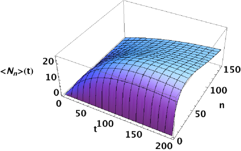
       (Color online)

Figure 1: (Left) (Color online) Starting from an initial pure BEC of $N=5000$ bosons, the plot shows the mean occupation number $\langle N_{n}\rangle(t)$ of state number $n$ ($n\neq 0)$ as a function of time $t$ (arbitrary units) due to CSL heating. We take $\lambda A^{2}=0.01$ and $\alpha=a/\sigma=0.1$, where $\sigma$ is the harmonic oscillator characteristic length $\sqrt{\hbar/m\omega}$. The energy $\varepsilon$ is related to occupation number via $\varepsilon=\hbar\omega n$. (Right) The exponential loss $\langle N_{0}\rangle(t)=N(0)e^{-\lambda A^{2}t}$ of the ground state with CSL heating.

IV Some Consequences of Rate Equations

We shall first discuss general properties of the rate equations. Then, we shall consider some detailed consequences.

When Eq.(17) is summed over $i$, the right hand side vanishes, reflecting the constant value of the total number of atoms $\equiv N$ in all states. This is because $\sum_{i}\gamma_{i}^{k}=0$, which follows from $\sum_{i}\varphi_{i}(\mathbf{y})\varphi_{i}^{*}(\mathbf{y}^{\prime})=\delta({\bf y}-{\bf y}^{\prime})$.

If $i=k$, the integrand in the definition of $\gamma_{i}^{i}$ is positive, which means that the CSL self-coupling coefficient of any population is always negative, corresponding to its decay.

Using the Fourier transform of the exponential in Eq.(18), $\gamma_{i}^{k}$ may be written as

$$\gamma_{i}^{k}=\delta_{ik}-\frac{a^{3}}{\pi^{3/2}}\int d{\bf q}e^{-{\bf q}^{2}a^{2}}\Big{|}\int d{\bf y}e^{i{\bf q}\cdot{\bf y}}\varphi_{i}(\mathbf{y})\varphi_{k}^{*}(\mathbf{y})\Big{|}^{2}.$$ (19)

Thus, if $i\neq k$, $\gamma_{i}^{k}$ is negative. By replacing $e^{-{\bf q}^{2}a^{2}}$ by 1 and performing the ${\bf k}$ integral, we obtain an upper bound on this term:

$$(2a\sqrt{\pi})^{3}\int d{\bf y}|\varphi_{i}(\mathbf{y})|^{2}|\varphi_{k}(\mathbf{y})|^{2}=C(a/\sigma)^{3}$$

where we take the scale of the wave function to be $\sigma$. Since it is assumed that $\sigma>>a$, according to Eq.(17), all initial state populations decay at a rate slightly less than $\lambda A^{2}$ but, in each interval $dt$, the $i$th state repopulates the rest (including itself) with a positive fraction $\sim\lambda A^{2}dt\langle N_{i}\rangle$.

It is an exact property of CSL that, regardless of the potential in the Hamiltonian, the mean energy of any system increases linearly with time. As shown in Appendix A:

$$\frac{d}{dt}\overline{E}=\lambda A^{2}N\frac{3\hbar^{2}}{4ma^{2}}.$$ (20)

So, the initial bound state distribution of the $N$ atoms gets excited at the rate $\lambda A^{2}$ with an average energy increase per atom $\sim\hbar^{2}/ma^{2}\equiv k_{B}T_{CSL}$, where $k_{B}$ is Boltzmann’s constant. If $a=10^{-5}$cm, for the two atoms ⁸⁷Rb and ¹³³Cs which are frequently used to form condensates, $k_{B}T_{CSL}$ has the respective values $\approx 550$nK and $\approx 360$nK.

IV.1 Bose-Einstein Condensate Without Thermal Cloud

Suppose one starts with all $N$ particles in the Bose-Einstein condensate ground state $\varphi_{1}(\mathbf{y})$, and sweeps away particles which are ejected (or achieves the same effect by making a very shallow trap with $T<<T_{CSL}$). Then, the rate equation (17) for $\langle N_{1}\rangle$ is to be modified so that the excited states do not inject atoms back into the BEC, and only the term $\gamma_{1}^{1}$ contributes :

$$\frac{d}{dt}\langle N_{1}\rangle=-\lambda A^{2}\Big{[}1-\int d\mathbf{y}\int d\mathbf{y}^{\prime}e^{-\left(\mathbf{y}-\mathbf{y}^{\prime}\right)^{2}/4a^{2}}|\varphi_{1}(\mathbf{y})|^{2}|\varphi_{1}(\mathbf{y}^{\prime})|^{2}\Big{]}\langle N_{1}\rangle.$$ (21)

Since the ground state wave function scarcely changes over the distance $a$, it is a good approximation to replace the exponential in Eq.(21) by a delta function, obtaining:

$$\frac{d}{dt}\langle N_{1}\rangle\approx-\lambda A^{2}\Big{[}1-a^{3}[4\pi]^{3/2}\int d\mathbf{y}|\varphi_{1}(\mathbf{y})|^{4}\Big{]}\langle N_{1}\rangle=-\lambda A^{2}\Big{[}1-[4\pi]^{3/2}C\Big{(}\frac{a}{\sigma}\Big{)}^{3}\Big{]}\langle N_{1}\rangle$$ (22)

where $C$ is of order 1: for a box of side length $\sigma$, $C=(3/2)^{3}$ and for a harmonic oscillator potential with $\sigma\equiv(m\omega)^{-1/2}$, $C=(2\pi)^{-3/2}$.

Thus, to an excellent approximation, the lifetime of the BEC due to the CSL process alone is $\tau_{CSL}\approx 1/(\lambda A^{2})$. If this experiment were to be performed, with a measured lifetime $\tau_{exp}$ resulting from the CSL process together with all other processes that limit the lifetime, since $\tau_{CSL}\geq\tau_{exp}$, that would place a limit

$$\lambda<1/(\tau_{exp}A^{2}).$$ (23)

For example, if the experiment was done with ¹³³Cs and the measured lifetime was $\tau_{exp}=10$s, the limit would be $\lambda<6\times 10^{-6}$s^-1.

The standard external optical or magneto-optical potential is harmonic, although recently a cylindrical box potential has been usedHadz . However, the effective potential is neither a box nor a harmonic oscillator potential. Usually a condensate is so dense that it creates a potential that dominates the trap’s harmonic oscillator potential near the center of the trap. The wave function in this case is given by solving the time-independent Schrödinger equation with both potentials, which is called the Gross-Pitaevskii equation. To a good approximation (called the Thomas-Fermi approximation), the squared wave function for a BEC atom isBaym

$$\phi_{0}^{2}({\bf y})=\frac{1}{\sigma^{3}}\Big{[}\Big{(}\frac{15}{8\pi}\Big{)}^{2/5}-\frac{{\bf y}^{2}}{\sigma^{2}}\Big{]}$$

where positive, and 0 for larger ${\bf y}^{2}$: $\sigma$ is a large multiple of the harmonic oscillator width. Putting this into (22), one obtains $C\approx 1.7$.

IV.2 Thermal Cloud Without Bose-Einsein Condensate

The atomic energy scale in a trap potential characterized by length $\sigma$ is $\hbar^{2}/m\sigma^{2}$ while the CSL energy scale is $\hbar^{2}/ma^{2}$. Since $\alpha\equiv a/\sigma<<1$, the CSL excitation covers many atomic states, so a sum over states can be well-approximated by an integral. For a sparse thermal cloud, the effective potential is the harmonic trap potential. If the thermal cloud is dense, and the atomic force is repulsive (which we shall assume, e.g., for ⁸⁷Rb and ¹³³Cs, the s-wave scattering length is positive), the effective potential tends to be flattened at the bottom, suggesting the utility of a calculation based upon a box potential.

For either the spherically symmetric harmonic oscillator potential with $\hbar\omega=\hbar^{2}/m\sigma^{2}$, or for the box with side length $\sigma$, we show in the appendices that both yield the same rate equations (B.1) or (B.2), for $\langle N_{\epsilon}\rangle$, the number of states per unit energy range,

$$\frac{d}{dt}\langle N_{\epsilon}\rangle=-\lambda A^{2}\langle N_{\epsilon}\rangle+\lambda A^{2}\frac{1}{\sqrt{\pi k_{B}T_{CSL}/2}}\int_{0}^{\infty}d\sqrt{\epsilon^{\prime}}\Big{[}e^{-\frac{2}{k_{B}T_{CSL}/2}(\sqrt{\epsilon}-\sqrt{\epsilon^{\prime}})^{2}}-e^{-\frac{2}{k_{B}T_{CSL}}(\sqrt{\epsilon}+\sqrt{\epsilon^{\prime}})^{2}}\Big{]}\langle N_{\epsilon^{\prime}}\rangle.$$ (24)

with solution Eq.(B.1)

$$\langle N_{\epsilon}\rangle(t) = \langle N_{\epsilon}\rangle(0)e^{-\lambda A^{2}t}$$

$$+ \frac{1}{\sqrt{\pi k_{B}T_{CSL}/2}}\int_{0}^{\infty}d\sqrt{\epsilon^{\prime}}\langle N_{\epsilon^{\prime}}\rangle(0)\sum_{s=1}^{\infty}e^{-\lambda A^{2}t}\frac{(\lambda A^{2}t)^{s}}{s!\sqrt{s}}\Big{[}e^{-\frac{2}{sk_{B}T_{CSL}}(\sqrt{\epsilon}-\sqrt{\epsilon^{\prime}})^{2}}-e^{-\frac{2}{sk_{B}T_{CSL}}(\sqrt{\epsilon}+\sqrt{\epsilon^{\prime}})^{2}}\Big{]}.$$

(25)

As expanded upon in Appendix B, this rate equation and solution are expected to be good approximations for any trap where the potential energy is negligibly small compared to the kinetic energy $k_{B}T_{CSL}$ for most of the spatial range of the wave function, which is the case for traps used in BEC experiments.

To illustrate Eq.(IV.2), Fig.2 displays the decay of an initial thermal cloud distribution into a time-dependent cloud generated by CSL heating. The energy $\varepsilon$ has been converted to occupation number via $\varepsilon=\hbar\omega n$.

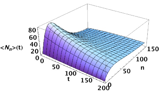
Figure 2: (Color online) Starting from an initial thermal cloud of $N=5000$ bosons at temperature $85$nK in a three-dimensional spherically symmetric harmonic trap, the plot shows the mean occupation number $\langle N_{n}\rangle(t)$ of state number $n$ as a function of time $t$ (arbitrary units) due to CSL heating. In this example, the transition temperature is $T_{c}=80.4$nK so there is no BEC, just a cloud. We take $\lambda A^{2}=0.01$, $T_{CSL}=500$ nK and $\alpha=\sqrt{\hbar\omega/k_{B}T_{CSL}}=.1$, so $\hbar\omega/k_{B}=5$nK.

This shows how the higher energy states are populated by the CSL heating mechanism as time increases. Interaction between the atoms has been disregarded here: of course, when it is included, the cloud continuously thermalizes and so may be characterized by an increasing temperature.

IV.3 Bose-Einstein Condensate and Thermal Cloud I

A common experimental situation is a BEC in thermal equilibrium with its surrounding cloud. We shall first consider the special case of noninteracting atoms in an anisotropic harmonic oscillator potential of infinite height. For completeness, its well known statistics are reviewed before use in our specific application.

The density of states is $\epsilon^{2}/2\overline{\omega}^{3}$, where $\epsilon$ is the system energy and $\overline{\omega}\equiv 2\pi(f_{1}f_{2}f_{3})^{1/3}$ (the oscillator’s three frequencies are $f_{1},f_{2},f_{3}$). The BEC occupies the ground state whose energy we take to be 0. If there are N atoms, Bose-Einstein statistics implies, below the critical temperature $T_{c}$, that the cloud contains $N_{cloud}<N$ atoms given by

$$N_{cloud}=\frac{1}{2\overline{\omega}^{3}}\int_{0}^{\infty}d\epsilon\frac{\epsilon^{2}}{e^{\frac{\epsilon}{k_{B}T}}-1}=\frac{1}{2}\Big{(}\frac{k_{B}T}{\overline{\omega}}\Big{)}^{3}\int_{0}^{\infty}dy\frac{y^{2}}{e^{y}-1}=\Big{(}\frac{k_{B}T}{\overline{\omega}}\Big{)}^{3}\zeta(3)$$ (26)

where $\zeta$ is the Riemann zeta function, with $\zeta(3)=1.20...$ . This calculation utilizes the approximation $\hbar\overline{\omega}<<k_{B}T$ in replacing the sum over discrete states by an integral over the density of states.

At the critical temperature $T_{c}$ below which the BEC forms, all the atoms are in the cloud so, from Eq.(26), we have

$$N=\Big{(}\frac{k_{B}T_{c}}{\overline{\omega}}\Big{)}^{3}\zeta(3).$$ (27)

Therefore, for $T<T_{c}$, from Eqs.(26),(27) it follows that

$$N_{cloud}=N\Big{(}\frac{T}{T_{c}}\Big{)}^{3},\qquad N_{BEC}=N\Big{[}1-\Big{(}\frac{T}{T_{c}}\Big{)}^{3}\Big{]}.$$ (28)

The condensate fraction is $f\equiv N_{BEC}/N$.

Similarly, Bose-Einstein statistics gives the cloud energy and specific heat/atom:

$$U_{cloud} = 3k_{B}T\Big{(}\frac{k_{B}T}{\overline{\omega}}\Big{)}^{3}\zeta(4)=N3k_{B}T_{c}\Big{(}\frac{T}{T_{c}}\Big{)}^{4}\frac{\zeta(4)}{\zeta(3)}$$

$$C \equiv \frac{1}{N}\Big{(}\frac{\partial U(T,N)}{\partial T}\Big{)}_{N}=\frac{1}{N}\Big{(}\frac{\partial U_{cloud}(T,N)}{\partial T}\Big{)}_{N}=12k_{B}\Big{(}\frac{T}{T_{c}}\Big{)}^{3}\frac{\zeta(4)}{\zeta(3)}$$ (29)

where $\zeta(4)=1.08...$ . Note that $U_{cloud}(T,N)$ depends only on $T$ because $T_{c}^{3}\sim N$.

Using conservation of energy, if only the CSL heating mechanism operates, the rate of increase of the CSL energy (20) equals the rate of increase of $U$:

$$N\lambda A^{2}\frac{3}{4}k_{B}T_{CSL}=\frac{d}{dt}U_{cloud}=NC\frac{dT}{dt}=NC\frac{dT}{df}\frac{df}{dt}=-\frac{NCf}{\tau_{f}df/dT}.$$ (30)

Eq.(30) has been expressed in terms of the lifetime $\tau_{f}$ of the condensate fraction:

$$\frac{1}{\tau_{f}}\equiv-\frac{1}{f}\frac{df}{dt}$$ (31)

because this is a readily measurable quantity. Inserting into (30) expression (IV.3) for $C$ and (28) for $F$, and solving for $\lambda$, we obtain

$$\lambda=\frac{1}{A^{2}\tau_{f}}\frac{T}{T_{CSL}}\Bigg{[}1-\Big{(}\frac{T}{T_{c}}\Big{)}^{3}\Bigg{]}\frac{16\zeta(4)}{3\zeta(3)}.$$ (32)

Therefore, were CSL to provide the only heating effect, one could measure $\lambda$ by measuring the BEC fraction lifetime and the temperature.

IV.4 Bose-Einstein Condensate and Thermal Cloud II

Atoms do interact, so the potential felt by each atoms is not just the harmonic oscillator potential of the trap. Reference Stringari-RMP considers an interacting Bose gas in the finite-temperature Hartree-Fock scheme with the Thomas-Fermi approximation for the condensate. The equations in the previous section are modified in this case as follows. The chemical potential $\mu$ is no longer 0:

$$\mu=k_{B}T_{c}\eta(1-s^{3})^{2/5}$$ (33)

where

$$\eta=\frac{\hbar\omega}{2k_{B}T_{c}}\left(\frac{15Na_{s}}{a_{HO}}\right)^{2/5}.$$ (34)

Here, $a_{HO}=\sqrt{\hbar/m\omega}$, $a_{s}$ is the atom-atom s-wave scattering length and $s\equiv T/T_{c}$: note that the critical temperature (at constant number of atoms) does not keep the same value as for an ideal gas, because of the change of density at the center of the trap induced by the interaction, but these equations use the expression (27) for the ideal gas $T_{c}$.

The condensate fraction is

$$f=1-s^{3}-\frac{\zeta(2)}{\zeta(3)}\eta s^{2}(1-s^{3})^{2/5}$$ (35)

and the energy is

$$U=Nk_{B}T_{c}\Bigg{\{}\frac{3\zeta(4)}{\zeta(3)}s^{4}+\frac{1}{7}\eta(1-s^{3})^{2/5}(5+16s^{3})\Bigg{\}}.$$ (36)

From Eqs.(35),(36) we can evaluate the following quantities:

$$C = \frac{1}{N}\Big{(}\frac{\partial U}{\partial T}\Big{)}_{N}=k_{B}\Bigg{\{}\frac{12s^{3}\zeta(4)}{\zeta(3)}+\frac{6s^{2}\eta}{\left(1-s^{3}\right)^{3/5}}\left(1-\frac{56s^{3}}{35}\right)\Bigg{\}}$$ (37)

$$\mu_{N} \equiv \Big{(}\frac{\partial U}{\partial N}\Big{)}_{T}=k_{B}T_{c}\frac{\eta}{5(1-s^{3})^{3/5}}(5+s^{3})$$ (38)

$$f_{T} \equiv \Big{(}\frac{\partial f}{\partial T}\Big{)}_{N}=-\frac{3s^{3}}{T}-\frac{2\eta\zeta(2)s^{2}}{5T\zeta(3)\left(1-s^{3}\right)^{3/5}}\left(5-8s^{3}\right)$$ (39)

$$f_{N} \equiv N\Big{(}\frac{\partial f}{\partial N}\Big{)}_{T}=s^{3}+\frac{\eta\zeta(2)s^{2}}{15\zeta(3)\left(1-s^{3}\right)^{3/5}}\left(9-15s^{3}\right)$$ (40)

In all cases, these expressions differ from those in the previous section by a term $\sim\eta$.

IV.5 Bose-Einstein Condensate and Thermal Cloud III

We now wish to obtain an expression for $\lambda$ similar to (32) for the case of interacting bosons and also now allow for the loss of atoms (change of $N$) as occurs in actual experiments. In so doing, the result shall be expressed in terms of practically measurable quantities.

The rate of increase of $U$ is given by

$$\frac{1}{N}\frac{d}{dt}U=C\frac{dT}{dt}+\mu_{N}\frac{1}{N}\frac{dN}{dt}$$ (41)

We shall evaluate this equation at $t=0$. Graphs of $N(t)$ and $f(t)$ may be experimentally obtained, from which the initial slopes may be extracted. These are defined as

$$\frac{1}{\tau_{N}} \equiv -\left.\left(\frac{1}{N}\frac{dN}{dt}\right)\right|_{t=0}$$ (42)

$$\frac{1}{\tau_{f}} = =-\left.\left(\frac{1}{f}\frac{df}{dt}\right)\right|_{t=0}$$ (43)

We do not assume the time dependence is strictly exponential for either $N$ or $f.$ We have

$$\left.\frac{df}{dt}\right|_{t=0}=-\frac{f(0)}{\tau_{f}}=f_{T}\left.\frac{dT}{dt}\right|_{t=0}+f_{N}\frac{1}{N}\left.\frac{dN}{dt}\right|_{t=0}$$ (44)

With all quantities evaluated at $t=0$, Eq. (44) implies that

$$\frac{dT}{dt}=\frac{1}{f_{T}}\left[\frac{f_{N}}{\tau_{N}}-\frac{f}{\tau_{f}}\right]$$ (45)

Substituting this into Eq. (41) gives

$$\frac{1}{N}\frac{dU}{dt}=\frac{C}{f_{T}}\left[\frac{f_{N}}{\tau_{N}}-\frac{f}{\tau_{f}}\right]-\frac{\mu_{N}}{\tau_{N}}$$ (46)

We emphasize that Eq.(46) is expressed in terms of experimental quantities and Hartree-Fock calculated quantities given in the previous section. It holds regardless of the specific mechanisms that heat or cool the atoms, or that remove atoms from the trap. In the following sections we shall calculate the contributions of various heating mechanisms in addition to that of CSL, and equate their energy change per particle to (46).

As a simple application, were there no other heating source other than CSL, as in Eq.(30), the rate of increase of the CSL energy (20) equals the rate of increase of $U$:

$$N\lambda A^{2}\frac{3}{4}k_{B}T_{CSL}=\frac{dU}{dt}.$$ (47)

It follows that the equivalent of Eq.(32) is

$$\lambda=\frac{4}{3}\frac{1}{A^{2}k_{B}T_{CSL}}\left\{\frac{C}{f_{T}}\left[\frac{f_{N}}{\tau_{N}}-\frac{f}{\tau_{f}}\right]-\frac{\mu_{N}}{\tau_{N}}\right\},$$ (48)

where the quantities in this equation are to be obtained from the Hartree-Fock expressions of the previous section. Of course, Eq.(48) is identical to Eq.(32) when $\eta=0$.

V CSL Heating with External Heating and Loss of Atoms

Naturally, in any actual experiment, in addition to heating from CSL, there will be other heating and cooling sources, and we consider this most general situation here. The heating processes we consider (the first two we found to be most significant) are as follows.

1) The rate of atoms in the cloud leaving the trap, with energy greater than the trap barrier height $\epsilon_{w}$, is $1/\tau_{cool}$. These processes are the source of evaporative cooling. The theory of Luiten et al LRW evaluates $\tau_{cool}$ and the cooling power, which we write as $(dU/dt)_{cool}$ (a negative quantity).

2) Three-body recombination (TBR) occurs when three atoms in the BEC inelastically collide, two forming a dimer, but all typically departing the trap when the barrier is low. BEC experiments usually try to minimize TBR losses. However, in the experimental data we examine, TBR is not negligible. Indeed, it is apparently the primary determinant of $\tau_{N}$ (dominating the particle number loss in 1) above), and contributes heating to the gas given by $(dU/dt)_{TBR}.$ We estimate the value of thisWeber . We find that, in order to fit the data, the TBR decay curve must be accompanied by a exponential tail at long times. We assume this tail is due to the evaporative cooling described in 1) above, and this gives us a value for $\tau_{cool}$.

3) Foreign atoms in the vacuum chamber, often mostly hydrogen, at essentially room temperature, occasionally collide with the atoms in the BEC or thermal cloud. With high probability, once struck, a Cs atom leaves the trap with no further collisions. We assume that the rate of atoms lost per atom, denoted $\tau_{1}^{-1}$, is the same for atoms in the BEC as it is for atoms in the thermal cloud. We denote the energy lost per atom as $-U_{av}/N\tau_{1}$, where $U_{av}$ is the average energy per atom in the system. $\tau_{1}$ can be estimated from the literatureBali .

4) Struck atoms which do not escape from the trap distribute their received energy.

5) Cs atoms removed from the trap may still occupy the neighborhood (the so-called “Oort cloud” Cornell ) and collide with trapped atoms.

6) Mechanical jitter of the laser beam focus which traps the atoms can heat them up. Intensity fluctuations of the laser beam have a similar effect.Savard

We shall denote by $R_{in}$ the rate of heating per atom due to CSL and sources 4)-6) (which we estimate as small but do not bother to provide the estimation here) and any other or unknown sources: the latter is basically what we will find as the residual in an experiment.

Then, equating the experimentally measurable energy change given by Eq.(46) to these listed sources of energy results in the relation

$$\frac{1}{N}\frac{dU}{dt}=R_{in}-\frac{1}{\tau_{1}}\frac{U_{av}}{N}+\frac{1}{N}\left.\frac{dU}{dt}\right|_{cool}+\frac{1}{N}\left.\frac{dU}{dt}\right|_{TBR}$$ (49)

with, of course, $dU/dt|_{cool}<0$. $R_{in}$ represents an upper limit on CSL heating so that

$$R_{in}=\frac{C_{N}}{f_{T}}\left[\frac{f_{N}}{\tau_{N}}-\frac{f}{\tau_{f}}\right]-\frac{\mu_{N}}{\tau_{N}}+\frac{1}{\tau_{1}}\frac{U_{av}}{N}-\frac{1}{N}\left.\frac{dU}{dt}\right|_{cool}-\frac{1}{N}\left.\frac{dU}{dt}\right|_{TBR}$$ (50)

and

$$\lambda<R_{in}\frac{4}{3A^{2}k_{B}T_{CSL}}.$$ (51)

VI Experimental Results

Hanns-Christoph Nägerl and Manfred Mark Mark of the University of Innsbruck have provided us with data for cesium condensates in four different optical traps. These data were gathered from their ongoing study of this system and the experiment was not designed with our purposes in mind. Thus while the limit we get on $\lambda$ is rather good, the result must be considered tentative, serving as a model for a more specific later experiment. Parameters of the traps are given in Table I:

Trap	freqs (Hz)	Depth (nK)	$a_{s}$ ($a_{0})$
1	20.5, 22.0, 30.0	158	232
2	14.3, 15.5, 21.1	79	232
3	22, 23.5, 32	158	250
4	15.5, 16.4, 22.6	79	250

Table I. Parameters for data for four cesium traps. The scattering length $a_{s}$ is given in units of the Bohr radius $a_{0}$.

We shall illustrate the calculation of the right-hand side of (50) with data from Trap 1 and present the results for the other three traps.

To begin, in order to calculate the contribution of $N^{-1}dU/dt$ (terms on the right-hand side of Eq.(46)), we need $\tau_{N}$ and $\tau_{f}$. We show below how we obtain these quantities, by fitting the $N(t)$ and $f(t)$ vs $t$ data with curves obtained by theoretical analysis of TBR and evaporative cooling.

We also need the values of $C$, $\mu_{N}$, $f_{T}$ and $f_{N}$. These are obtained from Hartree-Fock theory (as described by Dalfovo et al Stringari-RMP ), and are given at the end of section IVD. This approach has been found HKN to give results very close to Monte Carlo estimates.

Following this, we shall give a brief discussion of the estimates of the various energy sources for cooling and heating.

VI.1 Evaluation of $\tau_{N}$ from TBR and evaporative cooling

Three-body recombination in cesium has been extensively studied by the Innsbruck group Weber ; Kraemer ; Haller . The particle loss rate due to TBR is Burt

$$\frac{dN(t)}{dt}=-L_{3}\int d\mathbf{r}n^{3}(\mathbf{r},t)$$ (52)

where $n(\mathbf{r},t)$ is the particle density and $L_{3}$ is the rate of ejected particles; it is $3K_{3}$ where $K_{3}$ is the rate at which triples form if we assume that the trap height is small enough that all three particles are ejected. The parameter $K_{3}^{nc}$ for the non-condensate gas is 3! times larger than that for the condensate $K_{3}^{c}$ because of exchange terms for differing states.

When there is both a condensate with density $n_{0}(\mathbf{r})$ and a thermal cloud of density $n_{T}(\mathbf{r})$, the result is KSS

$$\frac{dN(t)}{dt}=-L_{3}^{c}\int d\mathbf{r}\left[n_{0}^{3}+9n_{0}^{2}n_{T}+18n_{0}n_{T}^{2}+6n_{T}^{3}\right]$$ (53)

with $L_{3}^{c}=3K_{3}^{c}$. The values of $K_{3}^{c}$ for cesium are given in Refs Kraemer ; Haller . Using the curves in Ref. Haller for pure cesium condensates we find, for $a_{s}=232a_{0}$, the value $K_{3}\approx 1.7\times 10^{-40}$m${}^{6}/$s. However for this $a_{s}$ value, Ref. Kraemer ’s study of thermal cesium gases finds a value about five times smaller.

To compute the rate (53), we use the finite-temperature Thomas-Fermi approximation for the condensate Stringari-RMP :

$$n_{0}(\mathbf{r})=\frac{1}{g}\left[\mu-V_{ext}({\bf r})\right]\theta(\mu-V_{ext}({\bf r}))$$ (54)

where $\theta(x)$ is the step function, $\mu$ is the chemical potential (33), $V_{ext}$ is the harmonic oscillator potential and $g=4\pi\hbar^{2}a_{s}/m$. The Hartree-Fock approximation for the thermal gas is:

$$n_{T}({\bf r})=\frac{1}{\lambda_{T}^{3}}g_{3/2}\left(\exp\left[-\beta\left(V_{ext}({\bf r})+2gn_{0}({\bf r})-\mu\right)\right]\right)$$ (55)

where the Bose integral is $g_{3/2}(z)=\sum_{l=1}^{\infty}z^{k}/k^{3/2}$, $\beta\equiv 1/k_{B}T$ and the thermal wavelength is $\lambda_{T}=\hbar\sqrt{2\pi/mk_{B}T}$. We have neglected the interaction between condensate and thermal cloud in $n_{0}$ and that between thermal atoms in $n_{T}$, so we do not have to iterate the equations.

It is to be expected that Eq.(53) is not accurate at large times. Then, the density at the origin becomes small so TBR is diminished, and evaporative cooling dominates. So we add a term $-N(t)/\tau_{cool}$ to the right hand side of (53) to account for that. Then, $N(t)$ is calculated and the best fit to the data is obtained by adjusting $K_{3}^{c}$, $N(0)$, and $\tau_{cool}$. In fitting the data for $N(t)$ we set the temperature at a value determined from the initial condensate fraction $f(0)$ (see below) and make the approximation that it does not change during the decay. This process is shown in Fig. 3 for Trap 1 where we find $\tau_{N}=24$ s. See Table II for the parameters from all four traps.

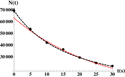
Figure 3: Decay of particle number (black dots) for a condensate plus thermal gas of Trap 1. The curve is fitted with a theory based on three-body recombination and evaporative cooling. We find parameters $K_{3}^{c}=3.6\times 10^{-41}$m⁶/s and $\tau_{cool}=62$ s. The fit also gives $N(0)=7.0\times 10^{4}$ and $\tau_{N}=18\pm 0.5$ s. A simple exponential fit is shown by the red dotted line.

The curve resulting from the TBR analysis plus the added exponential describing evaporative cooling appears to provide a considerably better fit to the data than the exponential alone: with just the latter, the best fit yields $\tau_{N}=24$s. Our value of $K_{3}^{c}$ is smaller than those expected from Ref. Haller but is near that found in Ref. Kraemer .

We find similar results for other traps provided by the Innsbruck group as shown in Table II.

VI.2 Evaluation of $\tau_{f}$

The other data we have to analyze is the condensate fraction. This is fit with an exponential as shown in Fig. 4. This is all that is needed. It is true that the condensate is the major contributor to the TBR losses because the TBR’s dependence is on density to the third power and the condensate is much more dense than the cloud. However, as the TBR process takes place, evaporative cooling and other particle loss in the thermal cloud also takes place, and re-thermalization restores particles to the condensate, causing $\tau_{f}$ to be much larger than $\tau_{N}$. We fit these cumulative complex processes with an exponential. The exponential fit gives not only $\tau_{f}$ but also $f(0)$ and from that $T$ via Eq. (35).

Figure 4: Decay of condensate fraction $f(t)$ (black dots) for a condensate plus thermal gas in Trap 1. An exponential best fit gives a decay constant $\tau_{f}=96$ s and $f(0)=0.76$. The latter parameter allows us to evaluate $T$.

Treating each of the four traps data sets in this way we can get a range of values for the parameters used in Eq.(46) to evaluate the initial value of $(1/N)dU/dt$ and the heating and cooling energy rates. We show the results in Table II.

Trap	$K_{3}$($10^{-41})$m6/s	$\tau_{cool}$(s)	$\tau_{N}$	$\tau_{f}$	$f(0)$	$T$	$N(0)$(104)	$T_{c}$(nK)
1	$3.6\pm 0.4$	$62\pm 12$	$17.5\pm 0.5$	$96\pm 9$	$0.76\pm 0.01$	$21\pm 0.6$	$7.0\pm 0.2$	$44$
2	$2.1\pm 0.6$	$43\pm 4$	$28\pm 1$	$383\pm 205$	$0.75\pm 0.02$	$16\pm$0.5	$8.3\pm 0.1$	$33$
3	$3.2\pm 0.1$	$67\pm 2$	$17.2\pm 0.1$	$61\pm 4$	$0.71\pm 0.02$	$25\pm 0.6$	$8.2\pm 0.1$	$50$
4	$3.5\pm 0.4$	$75\pm 10$	$24\pm 1$	$203\pm 31$	$0.82\pm 0.01$	$15\pm 0.4$	$9.0\pm 0.3$	$36$

$\mathbf{Caption}$: Table II. Ranges in fitted parameters to the data in four traps of the Innsbruck group.

VI.3 Energy sources

Next we turn to the contributions of the remaining three terms which make up $R_{in}$ in Eq.(50), evaporative cooling, TBR loss, and foreign atom collisions.

VI.3.1 Evaporative cooling

The LWR theory LRW of evaporative cooling is consistent with the more qualitative derivation of Pethick and Smith Pethick-book . While the expressions for $\tau_{cool}$ and $dU/dt|_{cool}$ given by LWR are somewhat involved we find that the cooling power is accurately summarized by the simple formula

$$\frac{1}{N}\frac{dU}{dt}_{cool}=-\frac{\alpha E_{B}}{\tau_{cool}}$$ (56)

where $E_{B}$ is the energy to escape the trap (trap height energy $\varepsilon_{w}$ minus zero-point energy) and $\alpha=1.12$. For Trap 1 the fitting of the $N(t)$ vs $t$ data gives $\tau_{cool}=35$s yielding the rate $-2.8$ nK/s.

VI.3.2 TBR heating

There are two references we know of that discuss the heating caused by three-body recombination Weber ; Werner . These both apply to thermal gases in the dilute (classical) limit where the kinetic energy cancels out of the problem and makes them inappropriate for our case of a mixed condensate and thermal gas. There is heating because the density cubed factor favors recombination in the center of the trap where the particles have lower energy. Thus, when these particles are ejected, each has less energy than the average energy per particle in the system. The excess energy left behind is shared among the remaining particles during re-equilibrization and is a heating effect. The particles near the center of the trap that are mostly involved in recombining are the condensate particles. Even with the Thomas-Fermi condensate wave function we have the condensate much nearer the center of the trap than the thermal particles. Moreover, we are concerned with condensate fractions of 0.70 to 0.80, which means the thermal density is small anyway. Thus the majority of particles taking part in the three-body recombination are condensate particles. However the thermal particles have larger energies and contribute more to the average energy. Thus we can estimate the energy lost per particle by TBR to be the energy per particle at $T=0,$ $E_{cond}=U(T=0)/N=\eta k_{B}T_{c}/7$ using Eq. (36) for the interacting energies. This is smaller than the average energy per particle $E_{av}=U(T)/N.$ So an estimate for the heating rate is

$$R_{TBR}=(E_{av}-E_{cond})/\tau_{N}$$ (57)

where, as before, $\tau_{N}$ is the initial particle number lifetime. Calculations for Trap 1 give a value of 0.6 nK/s.

VI.3.3 Foreign atom collisions and laser fluctuations

Bali et al Bali have estimated the collision rate between various foreign and trapped alkali atoms for shallow traps as a function of background gas pressure. The largest rate is due to Cs-Cs collisions. We might assume that lost cesium atoms stay in an “Oort cloud” Cornell and occasionally pass through the trapped gas. The estimated background gas pressure in the experiments we are analyzing is on the order of $2\times 10^{-11}$mbar Mark from which we can get the density of the background gas at 300K. We find that Cs-Cs collisions would occur at with a collision time of $\tau_{1}=320$ s. Collisions in which the trap atoms are not ejected from the trap lead to heating, which from Ref. Bali is on the order of $0.02$ nK/s, much too small to be relevant. If we assume all these collisions cause atoms to be ejected, then the energy rate contribution can be estimated as $-U_{av}/(N\tau_{1})$ where $U_{av}$ is the average energy in the trapped gas. This then yields a rate on the order of $-0.1$ nK/s, which is on the edge of being important. Of course if the background gas pressure were, say, ten times larger, this would be proportionately larger and be a major contributor.

Mark Mark has done a study of the fluctuations in position and intensity of the trapping lasers. Savard et al Savard shows that the laser positioning fluctuations give rise to a heating rate

$$\frac{d\left\langle E\right\rangle}{dt}=\frac{\pi}{2}m\omega_{tr}^{4}S(\omega_{tr})$$ (58)

where $\omega_{tr}$ is the trap frequency and $S(\omega_{tr})$ is the power spectral density of the positioning fluctuations; these reach a maximum of about $\sqrt{S}=6\times 10^{-3}$ $\mu$m/$\sqrt{\mathrm{Hz}}$ corresponding to a negligible heating($<0.02$nK/s).

VI.4 Summary

Table II shows the results from the four trap data sets. We use Eq.(50) to evaluate the unaccounted energy rate $R_{in}$, our upper limit on CSL heating. In the table, $\frac{1}{N}\frac{dU}{dt}$ is given by Eq.(46) and $W$, the sum of all the energy sources we have included in the computations, is the sum of the three columns before it. All energy rates are per particle.

TRAP	$\frac{1}{N}\frac{dU}{dt}$(nK/s)	$\frac{1}{N}\frac{dU}{dt}_{cool}$	$\frac{1}{N}\frac{dU}{dt}_{TBR}$	$\frac{-U_{av}}{\tau_{1}N}$	$W$	$R_{in}=\frac{1}{N}\frac{dU}{dt}-W$
1	$-1.4\pm 0.1$	$-2.8\pm 0.6$	$0.57\pm 0.06$	$-0.08$	$-2.3\pm 0.7$	$0.9\pm 0.7$
2	$-0.8\pm 0.1$	$-2.1\pm 0.2$	$0.28\pm 0.02$	$-0.06$	$-1.9\pm 0.2$	$1.1\pm 0.2$
3	$-1.6\pm 0.1$	$-2.6\pm 0.1$	$0.84\pm 0.03$	$-0.10$	$-1.9\pm 0.1$	$0.3\pm 0.2$
4	$-0.8\pm 0.1$	$-1.2\pm 0.2$	$0.23\pm 0.02$	$-0.05$	$-1.0\pm$0.2	$0.2\pm 0.2$

$\mathbf{Caption}$: Table III. Data estimates of results needed to evaluate $R_{in}$, the upper limit on the net energy input rate in the four traps.

Thus we have an average of $R_{in}=0.6\pm 0.5$ nK/s per particle. Using Eq.(51) we get a limit on $\lambda$ of

$$\lambda<1(\pm 1)\times 10^{-7}/\mathrm{s}$$ (59)

which is bested only by Fu’s limit $\lambda<1\times 10^{-9}/\mathrm{s}$ at presentFu .

In conclusion, we have presented an analysis of the heating of a Bose Einstein condensate according to the CSL theory of dynamical collapse. We have derived the relevant evolution of the density matrix, and thereby obtained rate equations describing the evolution of the population of atoms occupying the various energy levels in a bound state. We then applied this to the specific problem of a BEC and its attendant thermal cloud. We considered the other processes which compete with CSL heating in altering state populations in a practical experiment. Using data on cesium BEC’s kindly supplied by Hanns-Christoph Nägerl and Manfred Mark, we found an upper limit on the parameter $\lambda$ which governs the rate of collapse in the CSL theory.

Given the many uncertainties in our calculations, our result should be regarded as provisional, to be improved by an experiment of this kind specifically tailored to obtain a more precise energy audit and so reduce $R_{in}$ and its uncertainty and improve the limit on $\lambda$. Features of such an explicitly designed experiment would include heavy atomic mass (like cesium), low background of foreign atoms, systematic measurement of three-body recombination or its elimination, and a sufficiently high barrier to eliminate evaporative cooling as much as possible. An attractive possibility is to use a box boundary Hadz , which can have the advantage of a uniformly low density, minimizing interactions and three-body recombination and lengthening the BEC lifetime.

Appendix A Energy Increase

If the energy of the $i$th state is $\epsilon_{i}\equiv\langle\varphi_{i}|H|\varphi_{i}\rangle$, so $H={\bf P}^{2}/2m+V({\bf Y})=\sum_{i}\epsilon_{i}|\varphi_{i}\rangle\langle\varphi_{i}|$, the expression for the rate of increase of the ensemble-averaged energy, $\overline{E}\equiv\sum_{i}\epsilon_{i}\langle N_{i}\rangle$ follows from the rate equations (17), (18):

$$\frac{d}{dt}\overline{E} = -\lambda A^{2}\overline{E}+\lambda A^{2}\int d\mathbf{y}\int d\mathbf{y}^{\prime}e^{-(\mathbf{y}-\mathbf{y}^{\prime})^{2}/4a^{2}}\sum_{i}\epsilon_{i}\varphi_{i}(\mathbf{y})\varphi_{i}^{*}(\mathbf{y}^{\prime})\sum_{k}\varphi_{k}^{*}(\mathbf{y})\varphi_{k}(\mathbf{y}^{\prime})\langle N_{k}\rangle.$$

The sum over $i$ may be expressed as a matrix element of $H$, and then the exponential also can be expressed in terms of position operators:

$$\frac{d}{dt}\overline{E} = -\lambda A^{2}\overline{E}+\lambda A^{2}\int d\mathbf{y}\int d\mathbf{y}^{\prime}e^{-(\mathbf{y}-\mathbf{y}^{\prime})^{2}/4a^{2}}\langle{\bf y}|H|{\bf y}^{\prime}\rangle\sum_{k}\varphi_{k}^{*}(\mathbf{y})\varphi_{k}(\mathbf{y}^{\prime})\langle N_{k}\rangle$$ (61)

$$= -\lambda A^{2}\overline{E}+\lambda A^{2}\int d\mathbf{y}\int d\mathbf{y}^{\prime}\langle{\bf y}|e^{-(\mathbf{Y}_{L}-\mathbf{Y}_{R})^{2}/4a^{2}}H|{\bf y}^{\prime}\rangle\sum_{k}\varphi_{k}^{*}(\mathbf{y})\varphi_{k}(\mathbf{y}^{\prime})\langle N_{k}\rangle.$$

Expanding the exponential, the commutator with $H$ has only the non-vanishing part

$$\frac{d}{dt}\overline{E} = -\lambda A^{2}\overline{E}+\lambda A^{2}\int d\mathbf{y}\int d\mathbf{y}^{\prime}\langle{\bf y}|\{H-\frac{1}{4a^{2}}[{\bf Y},[{\bf Y},H]]\}|{\bf y}^{\prime}\rangle\sum_{k}\varphi_{k}^{*}(\mathbf{y})\varphi_{k}(\mathbf{y}^{\prime})\langle N_{k}\rangle.$$

The first term in the curly bracket cancels $-\lambda A^{2}\overline{E}$, since

$$\int d\mathbf{y}\int d\mathbf{y}^{\prime}\langle{\bf y}|H|{\bf y}^{\prime}\rangle\sum_{k}\varphi_{k}^{*}(\mathbf{y})\varphi_{k}(\mathbf{y}^{\prime})\langle N_{k}\rangle=\sum_{k}\langle\varphi_{k}|H|\varphi_{k}\rangle\langle N_{k}\rangle=\sum_{k}\epsilon_{k}\langle N_{k}\rangle=\overline{E}.$$

The commutator can readily be evaluated, with the result

$$\frac{d}{dt}\overline{E} = -\lambda A^{2}\frac{1}{4a^{2}}\int d\mathbf{y}\int d\mathbf{y}^{\prime}\langle{\bf y}|[{\bf Y},[{\bf Y},\frac{{\bf P}^{2}}{2m}]]|{\bf y}^{\prime}\rangle\sum_{k}\varphi_{k}^{*}(\mathbf{y})\varphi_{k}(\mathbf{y}^{\prime})\langle N_{k}\rangle$$ (63)

$$= \lambda A^{2}\frac{1}{4a^{2}}\frac{3}{2m}\int d\mathbf{y}\int d\mathbf{y}^{\prime}\delta({\bf y}-{\bf y}^{\prime})\sum_{k}\varphi_{k}^{*}(\mathbf{y})\varphi_{k}(\mathbf{y}^{\prime})\langle N_{k}\rangle=\lambda A^{2}N\frac{3}{4ma^{2}}.$$

using $\int d\mathbf{y}|\varphi_{k}(\mathbf{y})|^{2}=1$ and $\sum_{k}\langle N_{k}\rangle=N$. This linear increase of $\overline{E}$ with $t$ is a well-knownReviews consequence of CSL. It is often expressed as

$$\frac{d}{dt}\overline{E}=\lambda\frac{3}{4Ma^{2}}\frac{\cal M}{M}$$ (64)

where ${\cal M}$ is the total mass of all the atoms, and $M$ is the mass of a nucleon, which follows from Eq.(63) with use of $m=AM$ and ${\cal M}=MAN$.

Appendix B Rate Equations for Box and Harmonic Oscillator

For both a box potential with side length $\sigma$ and the harmonic oscillator with $m\omega=1/\sigma^{2}$, starting from the rate equations Eq.(17), (18):

$$\frac{d}{dt}\langle N_{i}\rangle=-\lambda A^{2}\langle N_{i}\rangle+\lambda A^{2}\sum_{k}\int d\mathbf{y}\int d\mathbf{y}^{\prime}e^{-\frac{1}{4a^{2}}(\mathbf{y}-\mathbf{y}^{\prime})^{2}}\varphi_{i}(\mathbf{y})\varphi_{i}^{*}(\mathbf{y}^{\prime})\varphi_{k}^{*}(\mathbf{y})\varphi_{k}(\mathbf{y}^{\prime})\langle N_{k}\rangle,$$ (65)

replace the state label $i$ by the indices $n_{1}n_{2}n_{3}$ to characterize the states $\phi_{n_{1}}(x)\phi_{n_{2}}(y)\phi_{n_{3}}(z)$, obtaining:

$$\frac{d}{dt}\langle N_{n_{1}n_{2}n_{3}}\rangle=-\lambda A^{2}\langle N_{n_{1}n_{2}n_{3}}\rangle+\lambda A^{2}\sum_{m_{1}m_{2}m_{3}}I_{n_{1}m_{1}}I_{n_{2}m_{2}}I_{n_{3}m_{3}}\langle N_{m_{1}m_{2}m_{3}}\rangle$$ (66)

where

$$I_{nm}\equiv\int dy\int dy^{\prime}\phi_{n}(y)\phi_{n}(y^{\prime})\phi_{m}(y)\phi_{m}(y^{\prime})e^{-\frac{1}{4a^{2}}[y-y^{\prime}]^{2}}.$$ (67)

B.1 Box

For the box, Eq.(67) becomes:

$$I_{nm} = \Big{(}\frac{2}{\sigma}\Big{)}^{2}\int_{0}^{\sigma}dy\int_{0}^{\sigma}dy^{\prime}\sin\frac{n\pi y}{\sigma}\sin\frac{n\pi y^{\prime}}{\sigma}\sin\frac{m\pi y}{\sigma}\sin\frac{m\pi y^{\prime}}{\sigma}e^{-\frac{1}{4a^{2}}[y-y^{\prime}]^{2}}$$ (68)

$$= \Big{(}\frac{2}{\pi}\Big{)}^{2}\int dx\int dx^{\prime}\sin nx\sin nx^{\prime}\sin mx\sin mx^{\prime}e^{-\frac{1}{4\alpha^{\prime 2}}[x-x^{\prime}]^{2}}.$$

where $\alpha^{\prime}\equiv\pi(a/\sigma)$. Because the exponential is large only for small $|x-x^{\prime}|\lesssim 2\alpha^{\prime}$, we make the approximation $\sin nx\sin nx^{\prime}=(1/2)[\cos n(x+x^{\prime})+\cos n(x-x^{\prime})]\approx(1/2)\cos n(x-x^{\prime})$, obtaining

$$I_{nm} \approx \Big{(}\frac{1}{\pi}\Big{)}^{2}\int_{0}^{\pi}dx\int_{0}^{\pi}dx^{\prime}\cos n(x-x^{\prime})\cos m(x-x^{\prime})e^{-\frac{1}{4\alpha^{\prime 2}}[x-x^{\prime}]^{2}}$$ (69)

$$= \frac{1}{2\pi^{2}}\int_{-\pi}^{\pi}dv\cos nv\cos mve^{-\frac{1}{4\alpha^{\prime 2}}v^{2}}\int_{v}^{2\pi-v}du$$

$$\approx \frac{1}{\pi}\int_{-\pi}^{\pi}dv\cos nv\cos mve^{-\frac{1}{4\alpha^{\prime 2}}v^{2}}$$

$$= \frac{1}{2\pi}\int_{-\infty}^{\infty}dv[\cos(n-m)v+\cos(n+m)v]e^{-\frac{1}{4\alpha^{\prime 2}}v^{2}}$$

$$= \frac{\alpha^{\prime}}{\sqrt{\pi}}\Big{[}e^{-(n-m)^{2}\alpha^{\prime 2}}+e^{-(n+m)^{2}\alpha^{\prime 2}}\Big{]}.$$

where in the second line we have changed variables to $v\equiv x-x^{\prime}$, $u\equiv x+x^{\prime}$, and in the third line we have used $\alpha^{\prime}<<\pi$.

Putting Eq.(69) into Eq.(66), we arrive at:

$$\frac{d}{dt}\langle N_{n_{1}n_{2}n_{3}}\rangle=-\lambda A^{2}\langle N_{n_{1}n_{2}n_{3}}\rangle+\lambda A^{2}\frac{\alpha^{\prime 3}}{(\pi)^{3/2}}\sum_{m_{1}m_{2}m_{3}}\prod_{k=1}^{3}\Big{[}e^{-\alpha^{\prime 2}(n_{k}-m_{k})^{2}}+e^{-\alpha^{\prime 2}(n_{k}+m_{k})^{2}}\Big{]}\langle N_{m_{1}m_{2}m_{3}}\rangle.$$

What we would like, however, are rate equations for the particle number in a state of given energy, i.e., for $\langle N_{n}\rangle\equiv\sum_{n_{1}n_{2}n_{3}}\langle N_{n_{1}n_{2}n_{3}}\rangle$ where the sum is over all $n_{i}$ such that $n=\sqrt{n_{1}^{2}+n_{2}^{2}+n_{3}^{2}}$ for the box (and $n=n_{1}+n_{2}+n_{3}$ for the harmonic oscillator). So, we evaluate Eq.(B.1) summed over all $n_{i}$ subject to the condition $n=[n_{1}^{2}+n_{2}^{2}+n_{3}^{2}]^{1/2}$:

$$S_{n} \equiv \frac{\alpha^{\prime 3}}{(\pi)^{3/2}}\sum_{n_{1}n_{2}n_{3}}\sum_{m_{1}m_{2}m_{3}}\prod_{k=1}^{3}\Big{[}e^{-\alpha^{\prime 2}(n_{k}-m_{k})^{2}}+e^{-\alpha^{\prime 2}(n_{k}+m_{k})^{2}}\Big{]}\langle N_{m_{1}m_{2}m_{3}}\rangle.$$ (71)

Setting $m\equiv[m_{1}^{2}+m_{2}^{2}+m_{3}^{2}]^{1/2}$, we approximate the sum over $n_{i}$ by an integral, obtaining:

$$S_{n} \equiv \frac{\alpha^{\prime 3}}{(\pi)^{3/2}}\sum_{m_{1}m_{2}m_{3}}e^{-\alpha^{\prime 2}[n^{2}+m^{2}]}J_{m_{1}m_{2}m_{3}}\langle N_{m_{1}m_{2}m_{3}}\rangle$$ (72a)

$$J_{m_{1}m_{2}m_{3}} \equiv \int_{0}^{n}dn_{1}dn_{2}dn_{3}\delta\Big{[}n-(n_{1}^{2}+n_{2}^{2}+n_{3}^{2})^{1/2}\Big{]}\prod_{k=1}^{3}\Big{[}e^{2\alpha^{\prime 2}n_{k}m_{k}}+e^{-2\alpha^{\prime 2}n_{k}m_{k}}\Big{]}$$ (72b)

To evaluate $J_{m_{1}m_{2}m_{3}}$, we switch to polar coordinates:

$$J_{m_{1}m_{2}m_{3}} = \int_{0}^{n}r^{2}dr\delta(n-r)\int_{0}^{\pi/2}d\theta\sin\theta\int_{0}^{\pi/2}d\phi$$ (73b)

$$\negthinspace\negthinspace\negthinspace\negthinspace\negthinspace\negthinspace\negthinspace\negthinspace\cdot 8\cosh(2\alpha^{\prime 2}nm_{3}\cos\theta)\cosh(2\alpha^{\prime 2}nm_{1}\sin\theta\cos\phi)\cosh(2\alpha^{\prime 2}nm_{2}\sin\theta\sin\phi)$$

$$= n^{2}\int_{0}^{\pi}d\theta\sin\theta\int_{0}^{2\pi}d\phi$$

$$\negthinspace\negthinspace\negthinspace\negthinspace\negthinspace\negthinspace\cdot\cosh(2\alpha^{\prime 2}nm_{3}\cos\theta)\cosh(2\alpha^{\prime 2}nm_{1}\sin\theta\cos\phi)\cosh(2\alpha^{\prime 2}nm_{2}\sin\theta\sin\phi)$$

The integral in Eq.(73b) is over the first quadrant, but the integral in Eq.(73b) is over all eight quadrants since, for the integral in any other quadrant, the $\sin$’s and $\cos$’s change sign, but the $\cosh$’s do not change. Upon writing $m_{i}=sv_{i}$, where ${\bf v}\cdot{\bf v}=1$, we see that the product of the $\cosh$’s is the sum of 8 terms, each of the form $\exp 2\alpha^{\prime 2}nm{\bf v}\cdot{\bf i}$, where ${\bf i}$ is a unit vector with (depending upon the term) components $\pm\sin\theta\cos\phi,\pm\sin\theta\sin\phi,\pm\cos\theta$. Since the integral is over the whole solid angle, we may in each case rotate the coordinate system, obtaining identical integrals for each, and thus

$$J_{m_{1}m_{2}m_{3}}=2\pi n^{2}\int_{-1}^{1}d\cos\theta e^{2\alpha^{\prime 2}nm_{1}\cos\theta}=\frac{n\pi}{m\alpha^{\prime 2}}\big{[}e^{2\alpha^{\prime 2}nm}-e^{-2\alpha^{\prime 2}nm}\big{]}$$ (74)

Putting Eq.(74) into Eq.(72a), and replacing the sum over $m$ by an integral, gives the result:

$$S_{n}=\frac{\alpha^{\prime}n}{\sqrt{\pi}}\int_{0}^{\infty}\frac{dm}{m}\Big{[}e^{-\alpha^{\prime 2}(n-m)^{2}}-e^{-\alpha^{\prime 2}(n+m)^{2}}\Big{]}\langle N_{m}\rangle.$$ (75)

Putting this into Eq.(B.1), we get the rate equations

$$\frac{d}{dt}\langle N_{n}\rangle=-\lambda A^{2}\langle N_{n}\rangle+\lambda A^{2}\frac{\alpha^{\prime}n}{\sqrt{\pi}}\int_{0}^{\infty}\frac{dm}{m}\Big{[}e^{-\alpha^{\prime 2}(n-m)^{2}}-e^{-\alpha^{\prime 2}(n+m)^{2}}\Big{]}\langle N_{m}\rangle.$$ (76)

Finally, we wish to express this as rate equations for the energy density of states $\langle N_{\epsilon}\rangle=\langle N_{n}\rangle dn/d\epsilon$. Using $n=\pi^{-1}\sigma\sqrt{2m\epsilon}$, we obtain

$$\frac{d}{dt}\langle N_{\epsilon}\rangle = -\lambda A^{2}\langle N_{\epsilon}\rangle+\frac{\lambda A^{2}}{\sqrt{\pi k_{B}T_{CSL}/2}}\int_{0}^{\infty}d\sqrt{\epsilon^{\prime}}\Big{[}e^{-\frac{2}{k_{B}T_{CSL}}(\sqrt{\epsilon}-\sqrt{\epsilon^{\prime}})^{2}}-e^{-\frac{2}{k_{B}T_{CSL}}(\sqrt{\epsilon}+\sqrt{\epsilon^{\prime}})^{2}}\Big{]}\langle N_{\epsilon^{\prime}}\rangle.$$

B.2 Harmonic Oscillator

For the harmonic oscillator, Eq.(67) becomes:

$$I_{nm} \equiv \int dy\int dy^{\prime}\phi_{n}(y)\phi_{n}(y^{\prime})\phi_{m}(y)\phi_{m}(y^{\prime})e^{-\frac{1}{4a^{2}}[y-y^{\prime}]^{2}}$$ (78)

$$= \frac{1}{\pi\sigma^{2}2^{n}2^{m}n!m!}\int dy\int dy^{\prime}e^{-\frac{y^{2}}{\sigma^{2}}}e^{-\frac{y^{\prime 2}}{\sigma^{2}}}H_{n}(y/\sigma)H_{n}(y^{\prime}/\sigma)H_{m}(y/\sigma)H_{m}(y^{\prime}/\sigma)e^{-\frac{1}{4a^{2}}[y-y^{\prime}]^{2}}$$

$$= \frac{1}{\pi 2^{n}2^{m}n!m!}\int dx\int dx^{\prime}e^{-x^{2}}e^{-x^{\prime 2}}H_{n}(x)H_{n}(x^{\prime})H_{m}(x)H_{m}(x^{\prime})e^{-\frac{1}{4\alpha^{2}}[x-x^{\prime}]^{2}},$$

where $\alpha\equiv a/\sigma<<1$. We shall use the asymptotic expression

$$H_{n}(x)\rightarrow e^{\frac{x^{2}}{2}}\sqrt{2^{n}n!}\Big{(}\frac{2}{\pi n}\Big{)}^{1/4}\cos\Big{(}x\sqrt{2n}-n\frac{\pi}{2}\Big{)}$$ (79)

(good to near the turning points at $x\approx\pm\sqrt{2n}$, and a fairly good approximation even for relatively small values of $n$) in Eq.(78):

$$I_{nm} \approx \frac{2}{\pi^{2}\sqrt{nm}}\int dx\int dx^{\prime}\cos\Big{(}x\sqrt{2n}-n\frac{\pi}{2}\Big{)}\cos\Big{(}x^{\prime}\sqrt{2n}-n\frac{\pi}{2}\Big{)}$$ (80a)

$$\qquad\qquad\qquad\qquad\cdot\cos\Big{(}x\sqrt{2m}-m\frac{\pi}{2}\Big{)}\cos\Big{(}x^{\prime}\sqrt{2m}-m\frac{\pi}{2}\Big{)}e^{-\frac{1}{4\alpha^{2}}[x-x^{\prime}]^{2}}$$

$$\approx \frac{1}{4\pi^{2}\sqrt{nm}}\int_{-c2\sqrt{2m}}^{c2\sqrt{2m}}du\int dv\cos\Big{(}v\sqrt{2n}\Big{)}\cos\Big{(}v\sqrt{2m}\Big{)}e^{-\frac{1}{4\alpha^{2}}v^{2}}$$ (80b)

$$= \alpha\frac{1}{\sqrt{2\pi n}}\Big{[}e^{-2\alpha^{2}(\sqrt{n}-\sqrt{m})^{2}}+e^{-2\alpha^{2}(\sqrt{n}+\sqrt{m})^{2}}\Big{]}$$ (80c)

In Eq.(80b), beside changing variables to $u\equiv x+x^{\prime}$, $u\equiv x-x^{\prime}$ and discarding the negligible oscillating cos terms which depend upon $u$ as in Appendix A, we have put in limits on the $u=x+x^{\prime}$ variable. This is because the approximation (79) is good only out to near the turning points $\pm\sqrt{2m}$, beyond which the $H_{m}$’s decay exponentially and give a negligible contribution. The constant $c$ is determined by the requirement that $\int_{0}^{\infty}dnI_{nm}=1$ (so particle number is constant), and is found to be $c=\pi/2$.

Putting Eq.(80c) into Eq.(66), we arrive at:

$$\frac{d}{dt}\langle N_{n_{1}n_{2}n_{3}}\rangle=-\lambda A^{2}\langle N_{n_{1}n_{2}n_{3}}\rangle+\lambda A^{2}\frac{\alpha^{3}}{(\pi)^{3/2}}\sum_{m_{1}m_{2}m_{3}}\prod_{k=1}^{3}\Big{[}e^{-2\alpha^{2}(n_{k}-m_{k})^{2}}+e^{-2\alpha^{2}(n_{k}+m_{k})^{2}}\Big{]}\langle N_{m_{1}m_{2}m_{3}}\rangle.$$

Next required is that we evaluate Eq.(B.2) summed over all $n_{i}$ subject to the condition $n=n_{1}+n_{2}+n_{3}$:

$$S_{n} \equiv \frac{\alpha^{3}}{(2\pi)^{3/2}}\sum_{n_{1}n_{2}n_{3}}\sum_{m_{1}m_{2}m_{3}}\frac{1}{\sqrt{n_{1}n_{2}n_{3}}}\prod_{k=1}^{3}\Big{[}e^{-2\alpha^{2}(\sqrt{n_{k}}-\sqrt{m_{k}})^{2}}+e^{-2\alpha^{2}(\sqrt{n_{k}}+\sqrt{m_{k}})^{2}}\Big{]}\langle N_{m_{1}m_{2}m_{3}}\rangle.$$

Setting $m\equiv m_{1}+m_{2}+m_{3}$, and summing over all $n_{i}$ corresponding to $n$, with the sum approximated by an integral, we have

$$S_{n} \equiv \frac{\alpha^{3}}{(2\pi)^{3/2}}\sum_{m_{1}m_{2}m_{3}}e^{-2\alpha^{2}[n+m]}J_{m_{1}m_{2}m_{3}}\langle N_{m_{1}m_{2}m_{3}}\rangle$$ (83a)

$$J_{m_{1}m_{2}m_{3}} \equiv \int_{0}^{p}\frac{dn_{1}dn_{2}dn_{3}}{\sqrt{n_{1}n_{2}n_{3}}}\delta(n-n_{1}-n_{2}-n_{3})\prod_{k=1}^{3}\Big{[}e^{4\alpha^{2}\sqrt{n_{k}m_{k}}}+e^{-4\alpha^{2}\sqrt{n_{k}m_{k}}}\Big{]}.$$ (83b)

To evaluate $J_{m_{1}m_{2}m_{3}}$, we first set $n_{k}=x_{k}^{2}$ and then switch to polar coordinates:

$$J_{m_{1}m_{2}m_{3}} = 8\int_{0}^{\sqrt{n}}dx_{1}dx_{2}dx_{3}\delta(n-x_{1}^{2}-x_{2}^{2}-x_{3}^{2})\prod_{k=1}^{3}\Big{[}e^{4\alpha^{2}x_{k}\sqrt{m_{k}}}+e^{-4\alpha^{2}x_{k}\sqrt{m_{k}}}\Big{]}$$ (84c)

$$= 8\int_{0}^{\infty}r^{2}dr\delta(n-r^{2})\int_{0}^{\pi/2}d\theta\sin\theta\int_{0}^{\pi/2}d\phi 8\cosh[4\alpha^{2}\sqrt{nm_{3}}\cos\theta]$$

$$\qquad\qquad\qquad\cdot\cosh[4\alpha^{2}\sqrt{nm_{1}}\sin\theta\cos\phi]\cosh[4\alpha^{2}\sqrt{nm_{2}}\sin\theta\sin\phi]$$

$$= 4\sqrt{n}\int_{0}^{\pi}d\theta\sin\theta\int_{0}^{2\pi}d\phi\cosh[4\alpha^{2}\sqrt{nm_{3}}\cos\theta]$$

$$\qquad\qquad\qquad\cdot\cosh[4\alpha^{2}\sqrt{nm_{1}}\sin\theta\cos\phi]\cosh[4\alpha^{2}\sqrt{nm_{2}}\sin\theta\sin\phi]$$

The integral in Eq.(84c) is over the first quadrant, but the integral in Eq.(84c) is over all quadrants since, for the integral in any other quadrant, the $\sin$’s and $\cos$’s change sign, but the $\cosh$’s do not change. Upon writing $m_{i}=mv_{i}^{2}$, where ${\bf v}\cdot{\bf v}=1$, we see that the product of the $\cosh$’s is the sum of 8 terms, each of the form $\exp 4\alpha^{2}\sqrt{nm}{\bf v}\cdot{\bf i}$, where ${\bf i}$ is a unit vector with (depending upon the term) components $nm\sin\theta\cos\phi,nm\sin\theta\sin\phi,nm\cos\theta$. Since the integral is over the whole solid angle, we may in each case rotate the coordinate system, obtaining

$$J_{m_{1}m_{2}m_{3}} = 8\pi\sqrt{n}\int_{-1}^{1}d\cos\theta e^{4\alpha^{2}\sqrt{nm}\cos\theta}=\frac{2\pi}{\alpha^{2}\sqrt{m}}\Big{[}e^{4\alpha^{2}\sqrt{nm}}-e^{-4\alpha^{2}\sqrt{nm}}\Big{]}.$$ (85)

Putting Eq.(85) into Eq.(83a) gives the result:

$$S_{n}=\frac{\alpha}{\sqrt{2\pi}}\int_{0}^{\infty}\frac{dm}{\sqrt{m}}\Big{[}e^{-2\alpha^{2}(\sqrt{n}-\sqrt{m})^{2}}-e^{-2\alpha^{2}(\sqrt{n}+\sqrt{m})^{2}}\Big{]}\langle N_{m}\rangle.$$ (86)

Putting this into Eq.(B.2), we get the rate equations

$$\frac{d}{dt}\langle N_{n}\rangle=-\lambda A^{2}\langle N_{n}\rangle+\lambda A^{2}\frac{\alpha}{\sqrt{2\pi}}\int_{0}^{\infty}\frac{dm}{\sqrt{m}}\Big{[}e^{-2\alpha^{2}(\sqrt{n}-\sqrt{m})^{2}}-e^{-2\alpha^{2}(\sqrt{n}+\sqrt{m})^{2}}\Big{]}\langle N_{m}\rangle$$ (87)

Finally, we wish to express this as rate equations for the energy density of states $\langle N_{\epsilon}\rangle=\langle N_{n}\rangle dn/d\epsilon$. Using $n=\epsilon/\omega=\epsilon m\sigma^{2}$, we obtain

$$\frac{d}{dt}\langle N_{\epsilon}\rangle = -\lambda A^{2}\langle N_{\epsilon}\rangle+\frac{\lambda A^{2}}{\sqrt{\pi k_{B}T_{CSL}/2}}\int_{0}^{\infty}d\sqrt{\epsilon^{\prime}}\Big{[}e^{-\frac{2}{k_{B}T_{CSL}}(\sqrt{\epsilon}-\sqrt{\epsilon^{\prime}})^{2}}-e^{-\frac{2}{k_{B}T_{CSL}}(\sqrt{\epsilon}+\sqrt{\epsilon^{\prime}})^{2}}\Big{]}\langle N_{\epsilon^{\prime}}\rangle.$$

Appendix C Solution of Rate Equations

The rate equations (B.2) and (B.1) are identical, despite their quite different potentials. This is because, in both cases, the bound state wave functions are sinusoids of fixed wave-number, or well approximated by sinusoids. That is a good approximation if the potential energy is negligible compared to the kinetic energy for most of the range of $x$ between the classical turning points. Since the natural energy range for CSL excitation is $k_{B}T_{CSL}$, which corresponds to sinusoid wavelengths of order $a$, these rate equations and the solution below hold well for a wide range of momenta around $k=2\pi/a$ and larger, for any trap where the potential energy is $<<k_{B}T_{CSL}$ for most of the range of $x$. This is true for the traps used in BEC experiments.

The solution of this rate equation can be found as follows. Set $\sqrt{\epsilon}\equiv z$, $\sqrt{\epsilon^{\prime}}\equiv z^{\prime}$ in (B.2) or (B.1), and assume that $\langle N_{\epsilon^{\prime}}\rangle$ is an antisymmetric function of $z^{\prime}$ (where it has not been previously defined) so that (B.2) or (B.1) may be written as

$$\frac{d}{dt}\langle N_{z}\rangle = -\lambda A^{2}\langle N_{z}\rangle+\frac{\lambda A^{2}}{\sqrt{\pi k_{B}T_{CSL}/2}}\int_{-\infty}^{\infty}dz^{\prime}e^{-\frac{2}{k_{B}T_{CSL}}(z-z^{\prime})^{2}}\langle N_{z^{\prime}}\rangle.$$ (89)

Apply the Fourier transform $g(k)\equiv\int_{-\infty}^{\infty}dze^{-ikz}\langle N_{z}\rangle$ to Eq.(89), with the result

$$\frac{d}{dt}g(k)=-\lambda A^{2}g(k)\Big{[}1-e^{-\frac{k^{2}k_{B}T_{CSL}}{8}}\Big{]}.$$ (90)

Solving for $g(k)$, and inverting the fourier transform, we obtain the solution to the rate equation, which can be written various ways:

$$\langle N_{\epsilon}\rangle(t) = \frac{1}{2\pi}e^{-\lambda A^{2}t}\int_{0}^{\infty}d\sqrt{\epsilon^{\prime}}\langle N_{\epsilon^{\prime}}\rangle(0)\int_{-\infty}^{\infty}dk\Big{[}e^{ik(\sqrt{\epsilon}-\sqrt{\epsilon^{\prime}})}-e^{ik(\sqrt{\epsilon}+\sqrt{\epsilon^{\prime}})}\Big{]}e^{\lambda A^{2}te^{-\frac{k^{2}k_{B}T_{CSL}}{8}}}$$

$$= \langle N_{\epsilon}\rangle(0)e^{-\lambda A^{2}t}$$

$$\negmedspace\negmedspace\negmedspace\negmedspace\negmedspace\negmedspace\negmedspace\negmedspace\negmedspace\negmedspace\negmedspace\negmedspace\negmedspace\negmedspace\negmedspace\negmedspace\negmedspace\negmedspace\negmedspace\negmedspace\negmedspace\negmedspace\negmedspace\negmedspace+\frac{1}{2\pi}e^{-\lambda A^{2}t}\int_{0}^{\infty}d\sqrt{\epsilon^{\prime}}\langle N_{\epsilon^{\prime}}\rangle(0)\int_{-\infty}^{\infty}dk\Big{[}e^{ik(\sqrt{\epsilon}-\sqrt{\epsilon^{\prime}})}-e^{ik(\sqrt{\epsilon}+\sqrt{\epsilon^{\prime}})}\Big{]}\Big{[}e^{\lambda A^{2}te^{-\frac{k^{2}k_{B}T_{CSL}}{8}}}-1\Big{]}$$

$$= \langle N_{\epsilon}\rangle(0)e^{-\lambda A^{2}t}$$

$$+ \frac{1}{\sqrt{\pi k_{B}T_{CSL}/2}}\int_{0}^{\infty}d\sqrt{\epsilon^{\prime}}\langle N_{\epsilon^{\prime}}\rangle(0)\sum_{s=1}^{\infty}e^{-\lambda A^{2}t}\frac{(\lambda A^{2}t)^{s}}{s!\sqrt{s}}\Big{[}e^{-\frac{2}{sk_{B}T_{CSL}}(\sqrt{\epsilon}-\sqrt{\epsilon^{\prime}})^{2}}-e^{-\frac{2}{sk_{B}T_{CSL}}(\sqrt{\epsilon}+\sqrt{\epsilon^{\prime}})^{2}}\Big{]}.$$

C.1 Conservation Laws

We now show that constant particle number and the proper linear energy increase are consequences of Eq.(25): this supports the validity of the approximations made in obtaining Eq.(B.1) or Eq.(B.2).

Multiply Eq.(25) by an arbitrary function $f(\epsilon)$, and integrate over all $\epsilon$ from 0 to $\infty$. Define $z=\sqrt{\epsilon}$ and, using $d\epsilon=2zdz$, one gets

$$\overline{f}(t) = \overline{f}(0)e^{-\lambda A^{2}t}$$ (92)

$$\negmedspace\negmedspace\negmedspace\negmedspace\negmedspace\negmedspace\negmedspace\negmedspace\negmedspace\negmedspace\negmedspace\negmedspace\negmedspace\negmedspace\negmedspace\negmedspace+\frac{1}{\sqrt{\pi k_{B}T_{CSL}/2}}\int_{0}^{\infty}d\sqrt{\epsilon^{\prime}}\langle N_{\epsilon^{\prime}}\rangle(0)\sum_{s=1}^{\infty}e^{-\lambda A^{2}t}\frac{(\lambda A^{2}t)^{s}}{s!\sqrt{s}}\int_{-\infty}^{\infty}2zdzf(z^{2})e^{-\frac{2}{sk_{B}T_{CSL}}(z-\sqrt{\epsilon^{\prime}})^{2}}$$

where $\overline{f}(t)\equiv\int_{0}^{\infty}d\epsilon f(\epsilon)\langle N_{\epsilon}\rangle(t)$.

If $f=1$, so $\overline{f}\equiv\langle N\rangle(t)$ is the total number of particles in all states, and $\langle N\rangle(0)\equiv N$, one obtains:

$$\langle N\rangle(t) = Ne^{-\lambda A^{2}t}$$ (93)

$$+\frac{1}{\sqrt{\pi k_{B}T_{CSL}/2}}\Big{[}1-e^{-\lambda A^{2}t}\Big{]}\int_{0}^{\infty}d\sqrt{\epsilon^{\prime}}\langle N_{\epsilon^{\prime}}\rangle(0)2\sqrt{\epsilon^{\prime}}\sqrt{\pi k_{B}T_{CSL}/2}=N$$

so particle number is conserved.

If $f=\epsilon=z^{2}$, so $\overline{f}(t)=\overline{E}(t)$, one obtains:

$$\overline{E}(t) = \overline{E}(0)e^{-\lambda A^{2}t}$$

$$+ \int_{0}^{\infty}d\sqrt{\epsilon^{\prime}}\langle N_{\epsilon^{\prime}}\rangle(0)\sum_{s=1}^{\infty}e^{-\lambda A^{2}t}\frac{(\lambda A^{2}t)^{s}}{s!}2\Big{[}3\sqrt{\epsilon^{\prime}}\frac{sk_{B}T_{CSL}}{4}+\epsilon^{\prime 3/2}\Big{]}$$

$$\negmedspace\negmedspace\negmedspace\negmedspace\negmedspace\negmedspace\negmedspace\negmedspace\negmedspace\negmedspace\negmedspace\negmedspace\negmedspace\negmedspace\negmedspace\negmedspace\negmedspace\negmedspace\negmedspace\negmedspace\negmedspace\negmedspace=\overline{E}(0)e^{-\lambda A^{2}t}+\int_{0}^{\infty}d\epsilon^{\prime}\langle N_{\epsilon^{\prime}}\rangle(0)\Big{[}\lambda A^{2}t\frac{3k_{B}T_{CSL}}{4}+\epsilon^{\prime}(1-e^{-\lambda A^{2}t})\Big{]}=N\lambda A^{2}t\frac{3k_{B}T_{CSL}}{4}+\overline{E}(0),$$

so the result is the linear energy increase Eq.(20).

C.2 Initial BEC

Consider an initial BEC of $N$ atoms and suppose an infinite box or harmonic trap. Then, the CSL excitation without collisions (and the attendant thermal equilibrium of the created cloud) is described by Eq.(25). Here, it is best to think of the BEC state as the sum of two terms, one the initially populated state which decays, and the other, the lowest member of the continuum of states. Using $\epsilon_{1}=\pi^{2}/2m\sigma^{2}=\alpha^{\prime 2}k_{B}T_{CSL}/2$, we obtain from Eq.(C3c):

$$\langle N_{\epsilon_{1}}\rangle(t) = Ne^{-\lambda A^{2}t},$$ (95a)

$$\langle N_{\epsilon}\rangle(t) = \frac{1}{\sqrt{\pi k_{B}T_{CSL}/2}}\int_{0}^{\infty}d\sqrt{\epsilon^{\prime}}N\delta(\epsilon^{\prime}-\epsilon_{1})\sum_{s=1}^{\infty}e^{-\lambda A^{2}t}\frac{(\lambda A^{2}t)^{s}}{s!\sqrt{s}}\Big{[}e^{-\frac{2}{sk_{B}T_{CSL}}(\sqrt{\epsilon}-\sqrt{\epsilon^{\prime}})^{2}}-e^{-\frac{2}{sk_{B}T_{CSL}}(\sqrt{\epsilon}+\sqrt{\epsilon^{\prime}})^{2}}\Big{]}$$ (95b)

$$= \frac{\alpha^{\prime}}{2\sqrt{\pi}\epsilon_{1}}N\sum_{s=1}^{\infty}e^{-\lambda A^{2}t}\frac{(\lambda A^{2}t)^{s}}{s!\sqrt{s}}\Big{[}e^{-\frac{\alpha^{\prime 2}}{s\epsilon_{1}}(\sqrt{\epsilon}-\sqrt{\epsilon_{1}})^{2}}-e^{-\frac{\alpha^{\prime 2}}{s\epsilon_{1}}(\sqrt{\epsilon}+\sqrt{\epsilon_{1}})^{2}}\Big{]}.$$

$$\approx \frac{2\alpha^{\prime 3}\sqrt{\epsilon}}{\sqrt{\pi}\epsilon_{1}^{3/2}}N\sum_{s=1}^{\infty}e^{-\lambda A^{2}t}\frac{(\lambda A^{2}t)^{s}}{s!s^{3/2}}e^{-\frac{\alpha^{\prime 2}}{s\epsilon_{1}}\epsilon},$$ (95c)

where, in obtaining Eq.(95c), the approximation $\epsilon_{1}<<\epsilon$ is made.

References

- (1) P. Pearle, Phys. Rev. A39, 2277 (1989).
- (2) G. C. Ghirardi, P. Pearle and A. Rimini, Phys. Rev. A42, 78 (1990).
- (3) P. Pearle in Open systems and measurement in relativistic quantum theory, F. Petruccione and H. P. Breuer eds., p.195 (Springer Verlag, Heidelberg 1999): A. Bassi and G. C. Ghirardi, Physics Reports 379, 257 (2003): P. Pearle in Journ. Phys. A: Math Theor. 40, 3189 (2007) and continued in Quantum Reality, Relativistic Causality and Closing the Epistemic Circle, eds. W. Myrvold and J. Christian (Springer, 2009), pp.257-292: A. Bassi, K. Lochan, S. Satin, T. P. Singh and H. Ulbricht, Revs. Mod. Phys. 85, 471 (2013).
- (4) G. C. Ghirardi, A. Rimini and T. Weber, Phys. Rev. D 34, 470 (1986); Phys. Rev. D36, 3287 (1987); Found. Physics 18, 1, (1988).
- (5) S. L. Adler, J. Phys. A: Math. Theor. 40: 2935-2957 (2007).
- (6) W. Feldmann, R. Tumulka, J. Phys. A: Math. Theor. 45, 065304 (2012).
- (7) This limit arises because free particles undergo random walk during collapse, and the resulting acceleration makes a charged particle radiate. FuFu calculated the rate of photon emission for an electron to be )counts/keV-sec counts/keV-sec, where , , is the electron mass and is the proton mass (see alsoAR ). Fu applied this rate to ”spontaneous” X-ray emission by the 4 valence electrons in Ge. With 8.24 atoms in a kg of Ge, the rate is counts/keV-kg-day. The inequality provides the upper limit . Improved data (drawn from Fig. 1 of the third reference in massp ) gives the experimental limit on spontaneous radiation appearing in a highly shielded 253g of Ge observed for 337 days as counts/.1keV-85.24kg-days, or (4.7,2.35)counts/keV-kg-day at keV respectively. Since for both data, the resulting limit is sec-1.
- (8) Q. Fu, Phys. Rev. A 56, 1806 (1997).
- (9) S. L. Adler and F. M. Ramazanoğlu, J. Phys. A40; 13395 (2007).
- (10) P. Pearle and E. Squires, Phys. Rev. Lett. 73; 1 (1994); B. Collett, P. Pearle, F. Avignone and S. Nussinov, Found. Phys.25, 1399 (1995); P. Pearle, J. Ring, J. I. Collar and F. T. Avignone, Found. Phys. 29, 465 (1999); G. Jones, P. Pearle and J. Ring, Found. Phys. 34, 1467 (2004).
- (11) C. Cohen-Tannoudji and D. Guery-Odelin, “Advances in atomic physics”, World Scientific (2011); see in particular Part 7.
- (12) F. Dalfovo, S. Giorgini, L. Pitaevskii and S. Stringari, Rev. Mod. Phys. 71, 463 (1999).
- (13) C.J. Pethick and H. Smith, “Bose-Einstein condensation in dilute gases”, Cambridge University Press (2008).
- (14) A.E. Reinhardt, T.A. Pasquini, M. Saba, A. Schirotzek, Y. Shin, D. Kielpinski, D.E. Pritchard and W. Ketterle, Science 301, 1513 (2003).
- (15) A. L. Gaunt, T. F. Schmidutz, I. Gotlibovych, R. P. Smith and Z. Hadzibabic, ArXiv 1212.4453v1.
- (16) G. Baym and C. J. Pethick, Phys. Rev. Lett. 76, 6 (1996).
- (17) O. J. Luiten, M. W. Reynolds, and J. T. M. Walraven,, “Kinetic theory of the evaporative cooling of a trapped gas,” Phys. Rev. 53, 381 (1996).
- (18) T. Weber, J. K. Herbig, M. Mark, H.C. Nägerl, and R. Grimm, Phys. Rev. Lett. 91,123201 (2003).
- (19) S. Bali, K. M. O’Hara, M. E. Gehm, S. R. Granade, and J. E. Thomas, “Quantum-diffractive background gas collisions in atom-trap heating and loss,” Phys. Rev. A 60, R29 (1999).
- (20) E. A. Cornell, J. R. Enser, and C. E. Weiman, in Proceedings of the International School of Physics “E. Fermi” Course CXL -Bose-Einstein Condensation in Atomic Gases, edited by M. Inguscio, S. Stringari, and C. E. Wieman, IOS Press (Amsterdam 1998). p. 15.
- (21) T. A. Savard, K. M. O’Hara, and J. E. Thomas, Phys. Rev. A 56, R1095 (1997).
- (22) M. Mark and H.-C. Nägerl, (private communication).
- (23) M. Holzmann, W. Krauth, and M. Naraschewski, Phys. Rev. A 59, 2956 (1999).
- (24) T. Kraemer, M. Mark, P. Waldburger, J. G. Danzl, C. Chin, B. Engeser, A. D. Lange, K. Pilch, A. Jaakkola, H.-C. Nägerl, and R. Grimm, Nature 440, 315 (2006).
- (25) E. Haller, M. Rabie, M. J. Mark, J. G. Danzl, R. Hart, K. Lauber, G. Pupillo, and H-C. Nägerl, Phys. Rev. Lett. 107, 230404 (2011).
- (26) E. A. Burt, R. W. Ghrist, C. J. Myatt, M. J. Holland, E. A. Cornell, and C. E. Wieman, Phys. Rev. Lett. 79, 337
- (27) Y. Kagan, B. V. Svistunov, and G. V. Shlyapnikov, JETP Lett. 42, 209 (1996). (1997).
- (28) B. S. Rem, A. T. Grier, I. Ferrier-Barbut, U. Eismann, T. Langen, N. Navon, L. Khaykovich, F. Werner, D. S. Petrov, F. Chevy, and C. Salomon, Phys. Rev. Lett. 110, 163202 (2013); Supplemental Information: (http://link.aps.org/ supplemental/10.1103/PhysRevLett.110.163202).