title section subsection subsubsection paragraph

Empirical Study of the 1–2–3 Trend Indicator

Abstract    In this paper we study automatically recognized trends and investigate their statistics. To do that we introduce the notion of a wavelength for time series via cross correlation and use this wavelength to calibrate the 1–2–3 trend indicator of [9] to automatically find trends. Extensive statistics are reported for EUR-USD, DAX-Future, Gold and Crude Oil regarding e.g. the dynamic, duration and extension of trends on different time scales.

Keywords    market technical trends, automatic trend analysis, wavelength of time series, autocorrelation

JEL classification    C19, C63

1 Introduction

If we take a look at an arbitrary financial time series, e.g. the chart of the DAX Future, it seems that the graph is affected by wavelike up and down movements, see Figure 1. Such movements are often used in e.g. trading systems or stopping criteria. This motivates us to study so called trends. Therefore we introduce the following notation of market mechanical up and down trends, basically going back to Charles H. Dow.

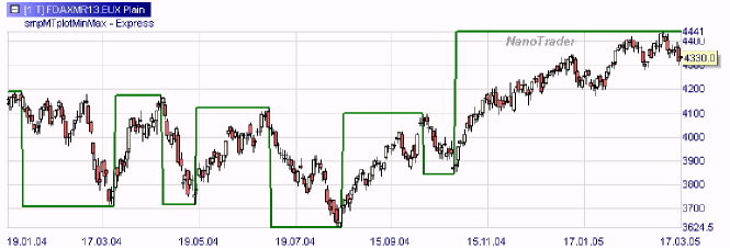
Figure 1: Snippet of the chart from DAX Future.

Definition 1.

(Market mechanical up/down Trends)
There is an up or down trend in a time series, if there is an increasing or a decreasing sequence of minima and maxima respectively, see Figure 2.

• Up trend: In this case the first extreme value must be a minimum, which we will call point 1. The second extreme value is a maximum (point 2) and the third one again a minimum (point 3). An up trend arises, if point 1 is below point 3 and the market price afterwards rises above the level of point 2, see Figure 2. The trend stays intact as long as the following extreme values are increasing minimal and maximal values.

• Down trend: This case is just a mirrored version of the up trend. It follows that point 1 is a maximum, point 2 a minimum and so on. As long as at least the last two minimal and last two maximal values are in a decreasing order, a down trend is active.

Figure 2: Up trend with numbering (cf. Definition 1) and two movements.

The time periods between these extreme values have special names.

Remark 1.

The period of time between point 2 and 3 is called correction phase, whereas one says movement phase for the time from point 3 to the succeeding point 2.

Trends are a gateway between the psychological behavior of the traders and the market mechanics. For a heuristic introduction see [2, 14]. Here we are interested in studying trends in a systematic way. For doing so it is important to understand the problematic of this definition of a trend or more specific the definition of a maximum and minimum. There are no rules to determine these minimal and maximal values. Therefore every arbitrary local extreme value can be used to identify trends, but clearly it is better when the extrema are “significant”. This problem is demonstrated in Figure 3, where we can see one to at most three extreme values with continuously increasing significance. In any case the definition of relevant extrema is a very subjective issue.

Figure 3: Continuation from one maximum to three extrema.

In [9] Maier-Paape describes a way to automatically generate a so called MinMax series out of a time series. Such a MinMax series is a sequence of alternating minima and maxima (see Figure 1, where the minimal and maximal values are emphasized by a line).

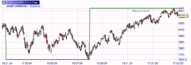
Figure 4: Chart of Figure 1 with other MinMax series.

The basic idea of the MinMax algorithm in [9] to find a MinMax process are so called SAR (stop and reverse) processes which are indicators that can have only the two different values “up” or “down”. For instance the MACD (moving average convergence/divergence) indicator of [1] can be used as SAR process. Simplified speaking, this process points up when the MACD series lies above its signal line and points down when its vice versa. Once the SAR process points up, the MinMax algorithm looks for a relevant maximum, and a relevant minimum is searched for, if the SAR process points down. See [9] for details. Together with Definition 1, trends can then be recognized automatically.

Of course the MACD indicator is controlled by parameters (default are $12$, $26$ and $9$) which in turn affect the SAR process and therefore also the extrema-induced trends. To obtain a one-dimensional controlling parameter, a common factor called “timescale” is used in the MinMax algorithm of [9] that scales the above default parameters of the MACD indicator simultaneously in order to accelerate or slow down the accompanying SAR process. In the following sections we will use only the MACD to induce the SAR process and use only the timescale parameter to adjust the trend behavior. For instance, if the timescale parameter is enlarged, fewer extreme are recognized by the MinMax algorithm (see Figure 4).

There is one subtlety, however: In order to avoid that the SAR process oscillates quickly in case MACD and signal line have multiple crossing points nearby, we adjust the SAR process slightly (for a change of the SAR process, the distance of MACD and signal line needs to be above some minimal threshold of $\delta=0.3\cdot\mbox{ATR}(100)$; see [9, Subsection 2.1] for details).

As mentioned above we want to study statistics of trends. Therefore we first set the timescale parameter in section 2 in a reasonable way. For doing so the “wavelength” of a chart is calculated in subsection 2.1 via cross-/autocorrelation. Then in subsection 2.2 with the help of the wavelength the MinMax algorithm is calibrated. The calculated trends are then analyzed in section 3.

Although we did intensive literature research, we were not able to find closely related work on automatic trend analysis which used a similar geometric trend definition via “MinMax processes”. Clearly, many other authors tried to design trading systems based on trends with miscellaneous results, see e.g. [5, 8, 13]. However, they do not use such a concrete definition of trends but define only some parameter dependent filter rules to trade up and down movements.

Acknowledgment This paper was funded as Seed Fund Project 2011/2012, RWTH Aachen.

2 Significant Period Length and Cross-Correlations

In the following we calculate the wavelength of a chart in subsection 2.1 via cross-/autocorrelation. Therefore we first introduce the corresponding notion and explain the calculation process. Afterwards the wavelength of some charts are presented. If the wavelength is known one can start calibrating the MinMax algorithm, see subsection 2.2. Therefore the interrelation between the principal parameter (timescale) of the MinMax algorithm and the wavelength is detected.

2.1 Wavelength of a Chart

Our first goal is to get a notion of a “wavelength” of a time series. Intuitively the wavelength should stand for some sort of natural fundamental oscillation of the price process of a chart. In the sequel we will try to adjust the MinMax algorithm such that the period length of the resulting extrema matches the wavelength. Here the period length is the average distance between two consecutive minimal or two maximal values in time. To determine the wavelength of a chart we want to use the idea of cross-correlations.

Assume $\mathbf{X}=(X_{t})_{t=0,...,N}\in\mathbb{R}^{N+1}$ and $\mathbf{Y}=(Y_{t})_{t=0,...,N}\in\mathbb{R}^{N+1}$ are two time series obtained from realizations of two stochastic processes. The empirical correlation $\phi\in[-1,1]$ of these two processes is then defined by

$$\phi:=\textnormal{Corr\,}(\mathbf{X},\mathbf{Y}):=\frac{\langle\mathbf{X},\mathbf{Y}\rangle}{\sqrt{\langle\mathbf{X},\mathbf{X}\rangle}\sqrt{\langle\mathbf{Y},\mathbf{Y}\rangle}},$$

where $\langle\cdot,\cdot\rangle$ is the euclidean inner product.

Similarly we define cross-correlation of a time series.

Definition 2.

(Cross-correlation/Autocorrelation)
Let $\mathbf{X}=\big{(}X_{t}\big{)}_{t\,\in\,\mathbb{N}_{0}}$ be the time series obtained from a stochastic process. We then call the empirical correlation of $\mathbf{Z}_{1}=\big{(}X_{t}\big{)}_{t\,=\,0,\ldots,N}$ and $\mathbf{Z}_{2}:=\mathbf{Z}_{2}^{n}:=(X_{t+n})_{t=0,...,N}$ for given $n,N\in\mathbb{N}$ the cross- or autocorrelation of $\mathbf{X}$ with time shift $n$.

In order to use the concept of the cross-correlation for the introduction of a wavelength of charts, we need to do some transformations.

A chart typically is of the form of a candle or bar chart, i.e. for one instant of time (one candle/bar) we get four values (open, close, high and low). The values open and close are the market values at a specific time, which are more or less randomized. However the values high and low are the maximum and minimum of a small period of time and therefore represent more than just one market price at a predefined point in time. For this reason we will use $\nicefrac{{(\text{high}+\text{low})}}{{2}}$ to get one value for each candle/bar, i.e. we use

$$a_{t} :=\frac{\text{high}(t)+\text{low}(t)}{2}, t\in\mathbb{N}_{0} \text{(used value for the }t\text{-th candle of the chart),}$$ (1)

as real valued time series representing the price process of the chart. In case (1) has some sort of a dominant wavelength $n^{*}$ after shifting $a_{t}$ by $n^{*}$ periods to the right (at least on average) maxima should more or less be close to maxima of the unshifted series and minima should be close to minima.

Unfortunately, even if this happens, we cannot directly measure that with the cross-correlation, since for instance two overlayed (positives) minima give a small contribution in the cross-correlation of Definition 2, whereas two overlayed maxima give a large contribution.

Therefore we have to do some modifications to obtain a large cross-correlation for the case that two maxima and minima clash and a small cross-correlation, if maxima hit minima. In order to obtain this behaviour, we subtract from (1) a moving average, such that an alleged minimum will be negative and an alleged maximum will be positive for the resulting series.

Of course the resulting maxima and minima of the new series will depend on the amount of periods we use for the moving average. It would be meaningful to take the moving average of the chart with a span of $n$ candles, where $n$ is equal or close to the dominant wavelength. However, since we do not know this dominant wavelength yet, we use $n$ for now as a parameter. To compute the average at one candle we will therefore take $\nicefrac{{n}}{{2}}$ periods in front of and $\nicefrac{{n}}{{2}}$ after the current candle. The difference of the real valued time series $a_{t}$ and its moving average becomes our time series $\mathbf{X}$, i.e. for

$$b_{t}^{n} :=\left(\frac{1}{2\lfloor\nicefrac{{n}}{{2}}\rfloor+1}\sum_{i=-\lfloor\nicefrac{{n}}{{2}}\rfloor}^{\lfloor\nicefrac{{n}}{{2}}\rfloor}a_{t+i}\right) a_{t} t\geq\lfloor\nicefrac{{n}}{{2}}\rfloor$$ (averaging of for )

we set

$$X_{t}^{n} :=a_{t}-b_{t}^{n}.$$ (2)

If our time series $(a_{t})_{t=0,...,M-1}$ is of length $M$, we now can compute the series $\mathbf{X}^{n}:=(X^{n}_{t})_{t=\lfloor\nicefrac{{n}}{{2}}\rfloor,...,M-1-\lfloor\nicefrac{{n}}{{2}}\rfloor}$ of length $M-2\lfloor\nicefrac{{n}}{{2}}\rfloor$. In Figure 5 one can see a chart, where the red line are the $a_{t}$ and the blue line $b_{t}^{n}$ for $t=1,...,81$ and $n=20$, where for the purpose of illustration our series $a_{t}$ is defined for $t\in\mathbb{Z}$. Since all values are positive, we obtain $X_{t}^{n}$ oscillating around zero, see Figure 6.

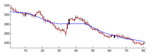
Figure 5: A chart with its values $a_{t}$ (red line) and $b_{t}^{n}$, $n=20$ (blue line).

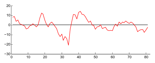
Figure 6: Plot of $X_{t}^{n}=a_{t}-b_{t}^{n}$, $n=20$, with $a_{t}$ and $b_{t}^{n}$ from Figure 5.

Now the cross-correlation will be large if we overlay two maxima or two minima (which now can be negative) in Definition 2.

Definition 3.

(“Cross-correlation” of a time series)
Let $A=(a_{t})_{t=0,...,M-1}$ be a real valued time series and $n\in\mathbb{N}$ be fixed. We define the cross-correlation of $A$ with time shift $n$ as

$$\phi_{n}:=\textnormal{Corr\,}(\mathbf{Z}_{1}^{n},\mathbf{Z}_{2}^{n}),$$

where $\textbf{Z}_{1}^{n}:=(X^{n}_{t})_{t=\lfloor\nicefrac{{n}}{{2}}\rfloor,...,N-\lfloor\nicefrac{{n}}{{2}}\rfloor}$ and $\textbf{Z}_{2}^{n}:=(X^{n}_{t+n})_{t=\lfloor\nicefrac{{n}}{{2}}\rfloor,...,N-\lfloor\nicefrac{{n}}{{2}}\rfloor}$ and $X_{t}^{n}$ as in (2). For a given shift $n$ we choose $N$ maximal, i.e. we use $N:=M-n-1$.

The $n$ with the largest cross-correlation will be called the dominant wavelength $n^{*}$ of the signal. In the next subsection the MinMax algorithm is adjusted such that it reproduces this dominant wavelength $n^{*}$.

In the left column of Figure 7 one sees the cross-correlation of the Chart of EUR-USD with different aggregations. The evaluation period used for the following studies is given in Table 2. From Figure 7 one approximately can extract the dominant wavelength, e.g. in the figure belonging to the day Chart of EUR-USD, the biggest extrema at $n^{*}=68$ probably marks the wavelength. In fact for $n=68$ the cross-correlation is largest with value $0.0966$. The range for lower $n$ shows oscillations, which are not meaningful. Similarly, the last big extremum which shows up between $n=200$ and $n=250$ corresponds to a multiple of the dominant wavelength of $n^{*}=68$. We proceed analogously with the remaining time units of EUR-USD in Figure 7. The corresponding dominant wavelengths were collected in Table 1. In addition in Table 1 are wavelengths for some other underlyings as well. Please note that although the cross-correlations are of small size there are still strong oscillations. Therefore one can assume that these values are meaningful.

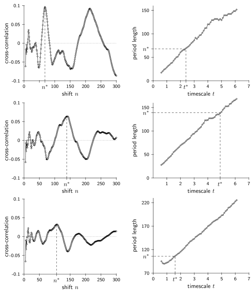
Figure 7: Euro US-Dollar: In the left column one sees the cross-correlation for values of $n$ between $1$ and $300$ and in the right column we plot the average period length one gets from the MinMax algorithm of [9] for different values of the timescale parameter. The aggregation is 1 day, 1 hour and 10 minutes from top to bottom. $n^{*}$ is the dominant wavelength and $t^{*}$ the corresponding timescale from Table 1 and 3, respectively.

Table 1: Some dominant wavelengths $n^{*}$ determined by the cross-correlation (evaluation time is given by Table 2).

		EUR-USD			FDAX			Gold			Crude Oil
Aggregation		$n^{*}$	Corr		$n^{*}$	Corr		$n^{*}$	Corr		$n^{*}$	Corr
1d		68	0.0966		101	0.0415		59	0.2550		86	0.0160
1h		139	0.0637		157	0.0600		112	0.0407		97	0.0401
10min		106	0.0322		59	0.0799		111	0.0701		64	0.0026

Table 2: Starting date for all studies (terminal date is always 25.01.2013). All historical data are from FIDES.

	EUR-USD	FDAX	Gold	Crude Oil
1d	15.07.1985	02.08.1993	14.09.1990	14.09.1990
1h	14.07.2009	17.12.1999	11.07.2005	29.11.2004
10min	03.01.2011	03.01.2011	03.01.2011	03.01.2011

2.2 Calibration of the MinMax algorithm

To adjust the trend finder according to the dominant wavelength $n^{*}$ given by subsection 2.1 it is necessary to detect the interrelation between the principle parameter (timescale) of the MinMax algorithm and the wavelength. One easy approach is to vary this parameter and compute for each fixed adjustment the averaged period length given by the relevant minima and maxima which we get from the trend finder. We will vary the timescale between $0.4$ and $6.0$ in $0.1$ steps. If we plot the resulting period length against the timescale, we get the result shown in the right column of Figure 7 for EUR-USD. In all three aggregations the dependence between timescale and observed average period length is close to (affine) linear. Now we can read the parameter for a given wavelength we got from subsection 2.1, see left column of Figure 7 for EUR-USD and Table 1. The values found for the timescale parameter $t^{*}$ that matches $n^{*}$ best can be found in Table 3.

Table 3: Choices for the timescale parameter $t^{*}$ to meet the dominant wavelength $n^{*}$.

Aggregation	EUR-USD	FDAX	Gold	Crude Oil
1d	2.4	3.7	2.2	3.4
1h	4.9	6.0	3.8	3.8
10min	1.6	1.6	2.5	1.6

The idea of calibrating the MinMax algorithm with the dominant wavelength of the chart fixes the relevant extrema and therefore also the “relevant” trends. We call this procedure according to [9] the 1–2–3 trend indicator. In the next section we want to verify the quality of this setting from a practical point of view. For example we can verify how long trends are active, i.e. how many maxima and minima are contained in the trends. The more maxima and minima we have for a trend on average the better the 1–2–3 trend indicator seems to work, because a trend with only two maxima and two minima is not helpful, because it disappears as quickly as it appeared. Before analysing basic statistical properties of trends we should do some remarks.

Remark 2.

1. The other local maxima in the plots of the cross-correlation of Figure 7 correspond to other – not so significant – wavelengths of the chart. After determining the respective timescales several in one other nested trends can be calculated. The study of these nested trends will however not be the subject of this paper.

2. As alternative way to determine relevant wavelengths/frequencies of a chart the empirical mode decomposition (EMD) [7] could be used. Dürschner used in [4] the EMD to analyse financial time series. Nevertheless, this method would not select a dominant wavelength.

3. Fourier Analysis and its (fast) Fourier transformation also provides a “frequency decomposition” and with it “strong modes”, see e.g. [10]. However, the comparison with this approach would be beyond the scope of this paper.

4. In this section we determined the cross-correlation from all available data. Alternatively one could calculate the cross correlations at each time $t$ from the last $T$ series points $(a_{s})_{s=t-T+1,...,t}$. This way the cross-correlation plots as well as $n^{*}$ and $t^{*}$ would depend on the time $t$, which might be more adapted to the actual market phase.

3 Basic Statistical Properties of Trends

Since we already fixed the parameter of the 1–2–3 trend indicator for each underlying, we now want to study trends in detail. The question is what kind of information about trends are important. Before we try to generate informations from trends which can help us for investment decisions we first should evaluate the quality of the detected trends. Therefore we define in subsection 3.1 two important measurement numbers, the dynamic and the lifetime of a trend. First we compare the corresponding results for different settings of the timescale on each underlying. If this analysis shows that the detected trends are meaningful we have a proper statistical basis of trends to work with. Therefore we analyze on this statistical basis complex chance and risk measurements in subsection 3.2 and discuss the expected values of these measurement numbers for each underlying using the fixed timescale from Table 3. In subsection 3.3 we then focus on the distribution of the dynamic to get a more detailed view on the shape of a trend.

3.1 How to measure trend quality

There are different methods to measure the strength of a trend. Classical methods to measure trend strength are e.g. the random walk index [12], the Aroon indicator [3] and the relative strength index (RSI) [15, 6]. All these indicators are applied directly to the price data of the chart and do not use our trend definition with P1, P2 and P3 explicitly. In this paper we therefore use the dynamic and the life-time of a trend.

Definition 4.

(Dynamic of a trend)
By dynamic we denote

$$\textnormal{dynamic}:=\frac{\textnormal{move. height}}{\textnormal{corr. height}}=\frac{|\textnormal{P2}_{\textnormal{new}}-\textnormal{P3}|}{|\textnormal{P2}-\textnormal{P3}|}>1,$$

i.e. the quotient of the height of the movement and the height of the preceding correction phase, see Figure 2 or Figure 8. Later for the statistics we always use the empirical expectation $\mathbb{E}(\textnormal{dynamic})$.

Figure 8: Situation of type 2–3–2 of Definition 6.

Remark 3.

In Figure 8 the last candle is marked with P2 id., which means that $\textnormal{P2}_{\textnormal{new}}$ is identified. Extrema are identified when the “status” series of the MinMax algorithm has changed, which of course is after the extrema occurred (see [9] for details).

The dynamic is very meaningful because it sets the movement phase in context to the correction phase. If this quantity takes a high value it is a good signal for the trend quality because this means that during the movement phase the price was increasing much and during the correction phase the price was decreasing less. In fact this is what a trader wants.

In the left column in Figure 9 the dynamic against the parameter timescale is shown. For day aggregation we see that the dynamic takes its maximal value of $2.31$ at a timescale of $2.6$. This timescale is nearly identical with $t^{*}$ we calculated from the dominant wavelength in section 2.1. For the other aggregations the values do not match that good, but if one ignores the values for timescale below one, the dynamic does not vary that much.

Figure 9: Euro US-Dollar: In the left column one sees the timescale plotted against the dynamic and in the right one sees the timescale against the number of movements. The aggregation is 1 day, 1 hour and 10 minutes from top to bottom and $t^{*}$ is the timescale from Table 3.

Another useful criterion for evaluating trends could be the life-time of a trend. This does not have a clear definition, e.g. it could mean the time under which the trend exists. This view seems not so meaningful because trends on a higher time scale would then usually live longer then those on a lower time scale. However, we will focus on characteristics of trends, that can be compared amongst various time scales. We therefore use the following definition.

Definition 5.

(Life-time of a trend)
We say a trend is long living if it consists of a lot of extremal values. We quantify this by the number of movements. This number is always at least two, since we also count the initial movement from P1 to P2, see Figure 2.

The reason for this point of view is that of course trends with a high number of movements are most meaningful for trading strategies. Thus we plot in the right column of Figure 9 the average number of movements per trend phase against the timescale. For the aggregation of 1 day and 1 hour the values $t^{*}$ for the timescale in Table 3 yields a good number of movements. For 10 minutes the number of movements does not vary much anyway.

So far it seems that our trend finder with the settings calculated from the wavelength is meaningful and therefore we will continue in the sequel always with the trend finder with timescale $t^{*}$.

3.2 Additional trend properties

We are now interested in collecting some basic properties of our trends which can help investors for investment decisions. For this reason we have to make some definitions.

Definition 6.

(Some properties of a trend)
The average true range (ATR), see [15], is the moving average of the true range

$$\textnormal{TR}:=\max\{\textnormal{high}-\textnormal{low},\textnormal{high}-\textnormal{close}[1],\textnormal{close}[1]-\textnormal{low}\},$$

where high and low means the high and low of the current period, respectively and close$[1]$ means the close of the previous period. Here the average of $100$ periods has been used. Assuming that a large average true range, i.e. a high volatility, leads to large movements and vice versa we use this value for normalization.

In the following we will distinguish between three different situations.

1–2–3:

We will call situations with identified points P1, P2 and P3 an 1–2–3, see Figure 10 left. In these situations no trend is active yet. If P3 is identified only after or during the break of the last P2, i.e. there is an active trend, we will ignore the situation, because such situations are not of use-oriented interest relating to the breakout of P2.

The number $\#(\textnormal{1--2--3})$ counts the number of situations which occur in the chart. We can use this property e.g. for forecasting how likely a trend will be generated after the occurrence of an 1–2–3.

Next we define

$$R_{\textnormal{1--2--3},\textnormal{ATR}} :=\frac{R_{\textnormal{1--2--3}}}{\textnormal{ATR(P3)}}:=\frac{\textnormal{close}(\textnormal{P3 ident.})-\textnormal{P3}}{\textnormal{ATR(P3)}} \text{(risk)},$$

$$G_{\textnormal{1--2--3},\textnormal{ATR}} :=\frac{G_{\textnormal{1--2--3}}}{\textnormal{ATR(P3)}}:=\frac{\textnormal{P2}-\textnormal{close}(\textnormal{P3 ident.})}{\textnormal{ATR(P3)}} \text{(goal)},$$

$$R_{\textnormal{1--2--3},\%} :=\frac{R_{\textnormal{1--2--3}}}{R_{\textnormal{1--2--3}}+G_{\textnormal{1--2--3}}}:=\frac{\textnormal{close}(\textnormal{P3 ident.})-\textnormal{P3}}{\textnormal{P2}-\textnormal{P3}} \text{(risk in \%)},$$

$$G_{\textnormal{1--2--3},\%} :=\frac{G_{\textnormal{1--2--3}}}{R_{\textnormal{1--2--3}}+G_{\textnormal{1--2--3}}}=1-R_{\textnormal{1--2--3},\%} \text{(goal in \%)},$$

which have to be positive for long-situations, see Figure 10 left. For short-situations, we use the absolute values of these expressions. The idea is that the occurrence of an 1–2–3 can be a trigger for a position entry suspecting a new trend with P1 as stop loss level and the last P2 as the smallest meaningful target.

Figure 10: Situations of type 1–2–3 (left) and 3–2–3 of Definition 6.

3–2–3:

Analogously we will call situations with identified points P3, P2 and $\textnormal{P3}_{\textnormal{new}}$ a 3–2–3, see Figure 10 right. In these situations a trend is already active, but the last P2 is not broken when the new P3 has been fixed. Otherwise we again ignore the situation for the same reason as for the 1–2–3 case.

The number of such situations are denoted by $\#(\textnormal{3--2--3})$ and we set again

$$R_{\textnormal{3--2--3},\textnormal{ATR}} :=\frac{R_{\textnormal{3--2--3}}}{\textnormal{ATR}(\textnormal{P3}_{\textnormal{new}})}:=\frac{\textnormal{close}(\textnormal{P3}_{\textnormal{new}}\textnormal{ ident.})-\textnormal{P3}_{\textnormal{new}}}{\textnormal{ATR}(\textnormal{P3}_{\textnormal{new}})} \textnormal{(}risk),$$

$$G_{\textnormal{3--2--3},\textnormal{ATR}} :=\frac{G_{\textnormal{3--2--3}}}{\textnormal{ATR}(\textnormal{P3}_{\textnormal{new}})}:=\frac{\textnormal{P2}-\textnormal{close}(\textnormal{P3}_{\textnormal{new}}\textnormal{ ident.})}{\textnormal{ATR}(\textnormal{P3}_{\textnormal{new}})} \textnormal{(}goal),$$

$$R_{\textnormal{3--2--3},\%} :=\frac{R_{\textnormal{3--2--3}}}{R_{\textnormal{3--2--3}}+G_{\textnormal{3--2--3}}}:=\frac{\textnormal{close}(\textnormal{P3}_{\textnormal{new}}\textnormal{ ident.})-\textnormal{P3}_{\textnormal{new}}}{\textnormal{P2}-\textnormal{P3}_{\textnormal{new}}} \text{(risk in \%)},$$

$$G_{\textnormal{3--2--3},\%} :=\frac{G_{\textnormal{3--2--3}}}{R_{\textnormal{3--2--3}}+G_{\textnormal{3--2--3}}}=1-R_{\textnormal{3--2--3},\%} \text{(goal in \%)},$$

which are positive for long-situations and otherwise we use the absolute values, see Figure 10 right.

2–3–2:

Situations where we know the points P2, P3 and the consecutive $\textnormal{P2}_{\textnormal{new}}>\textnormal{P2}$ of an active trend are called 2–3–2, see Figure 8. In these situations, we do not know the next minimum value, which might be a new P3 or – if below the old P3 – leads to a break of the trend.

In Definition 4 we already defined the dynamic of a trend. Another question is how much time is needed for a movement phase with respect to the time for the preceding correction phase. For this reason we first define the points with an additional time parameter. We say that P2 occurred at time $t2$, P3 at time $t3$ and $\textnormal{P2}_{\textnormal{new}}$ at time $t2_{\textnormal{new}}$. We then define

$$\textnormal{relative duration of dynamic}:=\frac{t2_{\textnormal{new}}-t3}{t3-t2}.$$

Since $\textnormal{P2}_{\textnormal{new}}$ is always identified with a time lag, see Remark 3, we are also interested in the effects of this delay. Therefore we define the lagged dynamics similar to the dynamic but we replace the point $(t2_{\textnormal{new}},\textnormal{P2}_{\textnormal{new}})$ with $(t2_{\textnormal{new,id}},\textnormal{close}(\textnormal{P2}_{\textnormal{new}}\textnormal{ ident.}))$, where $t2_{\textnormal{new,id}}$ is the time when $\textnormal{P2}_{\textnormal{new}}$ is identified, i.e. we have

lag. dyn $$:=\frac{|\textnormal{close}(\textnormal{P2}_{\textnormal{new}}\textnormal{ ident.})-\textnormal{P3}|}{|\textnormal{P2}-\textnormal{P3}|}$$

rel. duration of lag. dyn $$:=\frac{t2_{\textnormal{new,id}}-t3}{t3-t2}.$$

We note that the lagged dynamic does not have to be larger than one. These quantities are important because the identification point $t2_{\textnormal{new,id}}$ is immediately known as it occurs. In contrast the point $t2_{\textnormal{new}}$ always lies in the past when $\textnormal{P2}_{\textnormal{new}}$ is recognized and can therefore not be used directly.

Another important point is the break of P2. We denote the first candle which breaks $\textnormal{P2}_{\textnormal{break}}$, i.e. whose highest value is larger than P2, by the point $(\textnormal{t2}_{\textnormal{break}},\textnormal{P2}_{\textnormal{break}})$, see Figure 8. As above we define

rel. duration of break $$:=\frac{t2_{\textnormal{break}}-t3}{t3-t2}.$$

Remark 4.

1. We note that in both situations 1–2–3 as well as 3–2–3 there are possible countertrends when the succeeding situation breaks the last P3.

2. The probability that a trend breaks after a 2–3–2 can be computed by $\nicefrac{{\textnormal{\#trends}}}{{\textnormal{\#(2--3--2)}}}$, because the number of observed breaks equals the number of trends #trends (each trend breaks exactly one time) and #(2–3–2) gives us the number of all observed situations. Thus the probability of pass $\textnormal{P2}_{\textnormal{new}}$ after a 2–3–2 can be computed by

   $$1-\frac{\textnormal{\#trends}}{\textnormal{\#(2--3--2)}}.$$

Several properties of a trend are calculated for EUR-USD, DAX-Future, Gold and Crude Oil on different time-units, see Table 4 and Table 5. We tried to calculate them over a possibly huge period of time. Let us again mention that we used the dominant wavelength calculated in section 2.1 for calibrating the MinMax process and hence the 1–2–3 trend indicator, i.e. we used the timescale $t^{*}$ of Table 3. Now we discuss the results for the quantities of Definition 6 starting with the 1–2–3 situations.

1–2–3:

From Tables 4 and 5 we extract that for the highest time-unit, day base, only 44 situations of type 1–2–3 according to Definition 6 on the EUR-USD where found and only 16, 44 and 25 situations on the DAX-Future, Gold and Crude Oil respectively. In contrast there were 206 situations for the smallest time-unit on the EUR-USD and 206, 198 and 453 situations on the other underlyings within the evaluation period of our data. Of course the reason is the number of periods/candles used for the evaluations, which is lowest on day basis. Therefore we find most situations in the lowest time-unit.

The probability of activating a trend after a 1–2–3 situation is identified varies between only 28% and 62% on day basis and between 42% and 55% for intraday data. Of course the reason for the fluctuations of this value on day basis could be the small number of situations. Roughly speaking we have a 50% chance that a trend will occur after a 1–2–3.

The expectation of the risk $R_{\textnormal{1--2--3},\textnormal{ATR}}$ is always slightly higher or very close to the gain $G_{\textnormal{1--2--3},\textnormal{ATR}}$. This is confirmed by the relative risk $R_{\textnormal{1--2--3},\%}$, which is between 50% and 60%.

The last quantity for 1–2–3 situations is the expectation of the ratio of the height of the correlation and the height of the initial movement. This value is about 70%, which means that 70% of the initial price movement gets lost during the correction phase.

3–2–3:

The number of 3–2–3 situation is in all underlyings always observed smaller than the number of 1–2–3 situations. The probability of passing P2 after a 3–2–3 fluctuates between 28% and 65%, see Tables 4 and 5.

The values for the risk $R_{\textnormal{3--2--3},\textnormal{ATR}}$ and $R_{\textnormal{3--2--3},\%}$ and the gain $G_{\textnormal{3--2--3},\textnormal{ATR}}$ and also the quotient of the height of the correlation and the height of the preceding movement are very similar to the 1–2–3 setting.

2–3–2:

The probability of reaching a new P2 exceeding the old P2 under the condition that only the old P2, which is $\textnormal{P2}_{\textnormal{new}}$ in Figure 8, is identified by the 1–2–3 trend indicator increases significantly with rising the time-unit for the EUR-USD and also Crude Oil. This effect does not show up for the DAX-Future and Gold. For the Gold this quantity varies marginally with the time-units, so that the changes could be statistical fluctuations.

The dynamic gives us the quotient of the height of the movement and correction phase. A high dynamic means, that the market price will cover a large distance during the movement phase compared to the correction phase, which is more favorable. We see that the average dynamic takes its highest value for all underlyings except Crude Oil on day basis with a value above 2 in these three cases. In any case the average dynamic is above 1.75 which is also reasonably large.

For the relative duration of the dynamic, which is the quotient of the time needed for the movement phase and the time for the correction phase, this behavior is similar for the EUR-USD and the DAX-Future. The relative duration of the dynamic is much higher than the dynamic itself on all four underlyings, which means that the absolute value of the slope of the price changes is significantly higher for the correction than for the movement. This result is remarkable since movements are generally expected to be fast compared with corrections.

From the two quantities for the lagged dynamic one sees that the time between $\textnormal{P2}_{\textnormal{new}}$ and the identification of this point, which in general is part of the new correction, is larger than the time for the preceding correction phase. The lagged dynamic itself is about one, which means that the price of the chart on average goes back to the level of the old P2 before $\textnormal{P2}_{\textnormal{new}}$ is identified. Thus even the price changes after $\textnormal{P2}_{\textnormal{new}}$ are slightly slower than during the preceding correction.

The next two quantities $\mathbb{E}(\nicefrac{{\textnormal{move. height}}}{{\textnormal{ATR}(\textnormal{P}3)}})$ and $\mathbb{E}(\nicefrac{{\textnormal{corr. height}}}{{\textnormal{ATR}(\textnormal{P}3)}})$ in Tables 4 and 5 set the height of the movement, respectively the correction in context to the average true range, see Definition 6, at the last P3. The higher the value of $\mathbb{E}(\nicefrac{{\textnormal{move. height}}}{{\textnormal{ATR}(\textnormal{P}3)}})$ and the lower $\mathbb{E}(\nicefrac{{\textnormal{corr. height}}}{{\textnormal{ATR}(\textnormal{P}3)}})$ the better it is, because this means that the prices increased significantly during the movement phases and does not decrease much during the correction phase. We see that on average the height of the correction phase is slightly below 6 times and the height of the movement phase about 10 times the average true range. A very similar relation between these two values can be seen for $\mathbb{E}(\nicefrac{{\textnormal{move. height}}}{{\textnormal{low}(\textnormal{P}3)}})$ and $\mathbb{E}(\nicefrac{{\textnormal{corr. height}}}{{\textnormal{low}(\textnormal{P}3)}})$. One also can conclude that the DAX-Future and Crude Oil are comparably volatile, but Gold is less volatile and EUR-USD is the least volatile underlying.

Interestingly, on every time-unit trends in all underlyings have only very few movements numbers, which is slightly below $3$ on average.

Table 4: Some quality criteria for EUR-USD and DAX-Future with different aggregations.

underlying	EUR-USD			DAX-Future
time-unit	1d	1h	10min	1d	1h	10min
period of time from … to …	15.07.85	14.07.09	03.01.11	02.08.93	17.12.99	03.01.11
	25.01.13	25.01.13	25.01.13	25.01.13	25.01.13	25.01.13
number of candles	7151	21964	77235	4939	42622	44329
number of trends	33	59	299	18	93	286
$\#($1–2–3$)$	44	42	206	16	83	206
probability of	0.39	0.50	0.52	0.62	0.55	0.49
activate a trend
$\mathbb{E}(R_{\textnormal{1--2--3},\textnormal{ATR}})$	3.53	5.20	4.47	4.24	6.62	3.67
$\mathbb{E}(G_{\textnormal{1--2--3},\textnormal{ATR}})$	3.43	4.80	3.87	3.00	5.37	3.28
$\mathbb{E}(R_{\textnormal{1--2--3},\%})$	0.58	0.56	0.58	0.62	0.61	0.57
$\mathbb{E}(\frac{\textnormal{corr. height}}{\textnormal{ini. move. height}})$	0.69	0.76	0.70	0.64	0.73	0.73
$\#($3–2–3$)$	25	27	95	14	51	103
probability pass P2	0.60	0.52	0.40	0.50	0.65	0.39
after a 3–2–3
$\mathbb{E}(R_{\textnormal{3--2--3},\textnormal{ATR}})$	4.45	5.99	4.36	4.71	6.90	3.63
$\mathbb{E}(G_{\textnormal{3--2--3},\textnormal{ATR}})$	3.03	4.01	3.71	4.17	4.80	3.83
$\mathbb{E}(R_{\textnormal{3--2--3},\%})$	0.62	0.63	0.57	0.60	0.65	0.54
$\mathbb{E}(\frac{\textnormal{corr. height}}{\textnormal{move. height}})$	0.68	0.74	0.72	0.74	0.77	0.76
$\#($2–3–2$)$	69	104	472	32	187	495
probability pass P2	0.52	0.43	0.37	0.44	0.50	0.42
after a 2–3–2
$\mathbb{E}$(rel. dur. of break)	2.38	1.35	2.02	1.73	1.30	2.42
$\mathbb{E}$(rel. dur. of dyn.)	4.39	2.98	4.28	4.51	2.87	4.46
$\mathbb{E}$(dynamic)	2.18	1.82	1.88	2.15	1.75	2.09
$\mathbb{E}$(rel. dur. of	5.61	4.32	5.87	5.42	3.71	5.90
lag. dyn.)
$\mathbb{E}$(lag. dynamic)	1.36	1.08	0.97	1.36	0.99	1.16
$\mathbb{E}(\frac{\textnormal{move. height}}{\textnormal{ATR}(\textnormal{P}3)})$	9.88	12.22	9.66	11.83	13.66	8.34
$\mathbb{E}(\frac{\textnormal{corr. height}}{\textnormal{ATR}(\textnormal{P}3)})$	4.73	7.03	5.47	5.75	7.85	4.43
$\mathbb{E}(\frac{\textnormal{move. height}}{\textnormal{low}(\textnormal{P}3)})$	0.0873	0.0242	0.0079	0.2311	0.0778	0.0179
$\mathbb{E}(\frac{\textnormal{corr. height}}{\textnormal{low}(\textnormal{P}3)})$	0.0437	0.0141	0.0045	0.1186	0.0455	0.0096
$\mathbb{E}$(number of	3.09	2.76	2.58	2.78	3.01	2.73
movements)

Table 5: Some quality criteria for Gold and Crude Oil with different aggregations.

underlying	Gold			Crude Oil
time-unit	1d	1h	10min	1d	1h	10min
period of time from … to …	14.09.90	11.07.05	03.01.11	14.09.90	29.11.04	03.01.11
	25.01.13	25.01.13	25.01.13	25.01.13	25.01.13	25.01.13
number of candles	5632	42901	74356	5622	44907	74310
number of trends	33	136	258	20	170	458
$\#($1–2–3$)$	44	122	198	25	142	453
probability of	0.43	0.46	0.42	0.28	0.49	0.48
activate a trend
$\mathbb{E}(R_{\textnormal{1--2--3},\textnormal{ATR}})$	3.56	4.94	4.36	4.52	5.39	3.23
$\mathbb{E}(G_{\textnormal{1--2--3},\textnormal{ATR}})$	3.66	5.15	4.25	3.79	4.16	3.47
$\mathbb{E}(R_{\textnormal{1--2--3},\%})$	0.53	0.53	0.56	0.59	0.60	0.54
$\mathbb{E}(\frac{\textnormal{corr. height}}{\textnormal{ini. move. height}})$	0.71	0.72	0.68	0.71	0.75	0.66
$\#($3–2–3$)$	20	61	114	12	73	163
probability pass P2	0.40	0.43	0.44	0.58	0.44	0.28
after a 3–2–3
$\mathbb{E}(R_{\textnormal{3--2--3},\textnormal{ATR}})$	4.50	5.08	4.93	4.55	5.32	3.52
$\mathbb{E}(G_{\textnormal{3--2--3},\textnormal{ATR}})$	3.42	5.37	4.82	3.65	4.28	4.39
$\mathbb{E}(R_{\textnormal{3--2--3},\%})$	0.60	0.54	0.55	0.60	0.61	0.49
$\mathbb{E}(\frac{\textnormal{corr. height}}{\textnormal{move. height}})$	0.75	0.75	0.69	0.76	0.73	0.67
$\#($2–3–2$)$	61	252	435	38	302	720
probability pass P2	0.46	0.46	0.41	0.47	0.44	0.36
after a 2–3–2
$\mathbb{E}$(rel. dur. of break)	1.52	2.54	3.60	1.66	2.90	2.97
$\mathbb{E}$(rel. dur. of dyn.)	3.21	4.21	5.35	3.14	5.27	4.59
$\mathbb{E}$(dynamic)	2.07	1.86	2.02	1.81	1.77	2.06
$\mathbb{E}$(rel. dur. of	4.41	5.63	7.12	4.33	6.69	6.05
lag. dyn.)
$\mathbb{E}$(lag. dynamic)	1.15	1.09	1.06	0.90	0.98	1.09
$\mathbb{E}(\frac{\textnormal{move. height}}{\textnormal{ATR}(\textnormal{P}3)})$	9.71	11.96	11.63	10.34	10.81	9.03
$\mathbb{E}(\frac{\textnormal{corr. height}}{\textnormal{ATR}(\textnormal{P}3)})$	5.23	6.63	6.15	5.77	6.35	4.66
$\mathbb{E}(\frac{\textnormal{move. height}}{\textnormal{low}(\textnormal{P}3)})$	0.1209	0.0431	0.0143	0.3026	0.0655	0.0173
$\mathbb{E}(\frac{\textnormal{corr. height}}{\textnormal{low}(\textnormal{P}3)})$	0.0649	0.0240	0.0076	0.1733	0.0383	0.0091
$\mathbb{E}$(number of	2.85	2.85	2.69	2.90	2.78	2.57
movements)

3.3 Position of the new P2 for 2–3–2

In the last subsection we only used the (empirical) expectation to study the arithmetic mean of the observed quantities. Of course the expectation by itself does not tell us the whole truth. Values can have large fluctuations so that the expectation is less meaningful. However, we can not give a full discussion on all quantifies of Table 4 and Table 5. Hence we will concentrate on one of the most important quantities which is the dynamic of 2–3–2 situations.

In Figure 11 one sees the relative frequency distribution of the dynamic for all four underlyings. We can see, that the dynamic is concentrated between a value of 1 and 2.5 and there are even values which are greater of equal to 4. On 1 day basis there is a noticeable large number of situations with a dynamic of 4 and larger on the EUR-USD, DAX-Future and Gold while there is none for the Crude Oil. This tells us that especially on DAX-Future and Gold stable long term trends are possible. The frequency distributions for 1h and 10min look more smooth. Here on 10min basis the dynamic also can be greater or equal to 4 with a probability of at least 5%, while the probability for 1h time aggregation is always below 5%. This is the most significant difference between the distribution of different time aggregations, which of course effects the expectation of the dynamic, see Tables 4 and 5. In Gold on day basis the number of 2–3–2 situations with very small dynamics is extremely large. A lot of movements are killed right away which could be caused by possible market manipulations. All distributions in Figure 11 look approximately like Log-normal distributions.

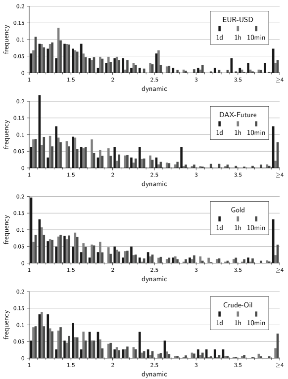
Figure 11: Frequency distribution of the dynamics, i.e. the relative positions of $\textnormal{P2}_{\textnormal{new}}$ in a situation of type 2–3–2 of Definition 6.

Besides the dynamic the relative duration of the dynamic, i.e. the relative duration of the movement phase, is needed to identify the position of $\textnormal{P2}_{\textnormal{new}}$ in 2–3–2 Situations. Since a large dynamic is preferable we are interested in the probability of exceeding a given value. We therefore do not use the cumulative distribution function in the classical sense, but we use the probability of a position of the new P2 which has a dynamic and a relative duration of dynamic larger than given values, i.e. we use

$$\tilde{F}(x,y):=\mathbb{P}\left(\textnormal{rel. duration of dyn.}\geq x,\,\,\textnormal{dynamic}\geq y\right)$$ (3)

for $x\geq 0$ and $y\geq 1$. From Tables 4 and 5 we directly get the expectation of this two dimensional distribution, which is defined by the expectations of each component, i.e.

$$\mathbb{E}\left(\left[\begin{matrix}\textnormal{rel. duration of dyn.}\\ \textnormal{dynamic}\end{matrix}\right]\right) :=\left[\begin{matrix}\mathbb{E}(\textnormal{rel. duration of dyn.})\\ \mathbb{E}(\textnormal{dynamic})\end{matrix}\right],$$ (4)

see e.g. [11, Definition 3.3]. Analogously one can define the expectations for $\textnormal{P2}_{\textnormal{break}}$ and the identification of $\textnormal{P2}_{\textnormal{new}}$ by

$$\mathbb{E}\left(\left[\begin{matrix}\textnormal{rel. dur. of break}\\ \textnormal{``dynamic of break''}\end{matrix}\right]\right) :=\left[\begin{matrix}\mathbb{E}(\textnormal{rel. dur. of break})\\ 1\end{matrix}\right]$$ (5)

$$\text{and}\qquad\mathbb{E}\left(\left[\begin{matrix}\textnormal{rel. dur. of lag. dyn.}\\ \textnormal{lag. dynamic}\end{matrix}\right]\right) :=\left[\begin{matrix}\mathbb{E}(\textnormal{rel. dur. of lag. dyn.})\\ \mathbb{E}(\textnormal{lag. dynamic})\end{matrix}\right].$$ (6)

In Figures 12 and 13 the reversed cumulative distribution function from (3) is plotted for the EUR-USD, DAX-Future, Gold and Crude Oil, respectively, for all three time aggregations. The shape looks quite similar for all these functions. One clearly sees that the probability of a long duration of the movement phase is much higher than the probability of a high move. Another observation is that the velocities of the price value on average are roughly the same for the move from P3 to $\textnormal{P2}_{\textnormal{break}}$ and from $\textnormal{P2}_{\textnormal{break}}$ to $\textnormal{P2}_{\textnormal{new}}$. This means that the whole movement is slow compared to the correction phase.

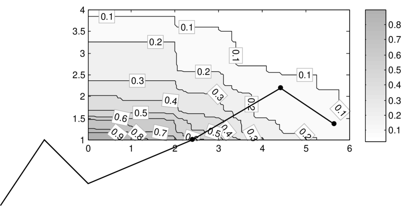
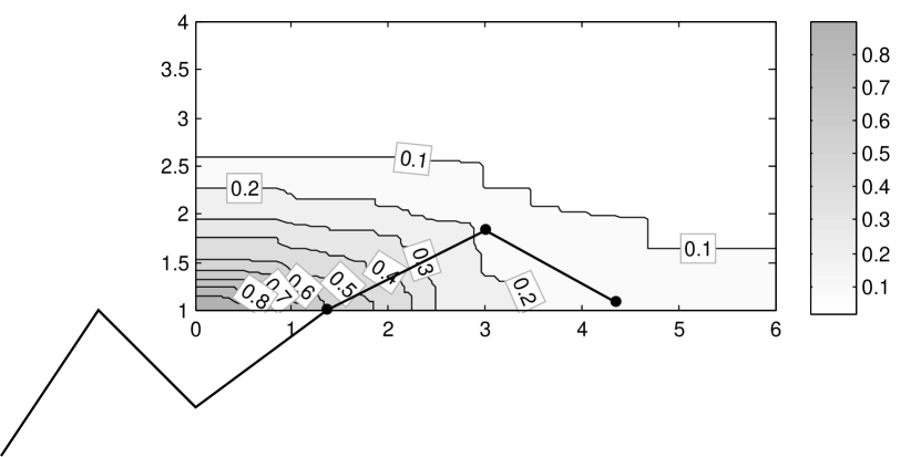
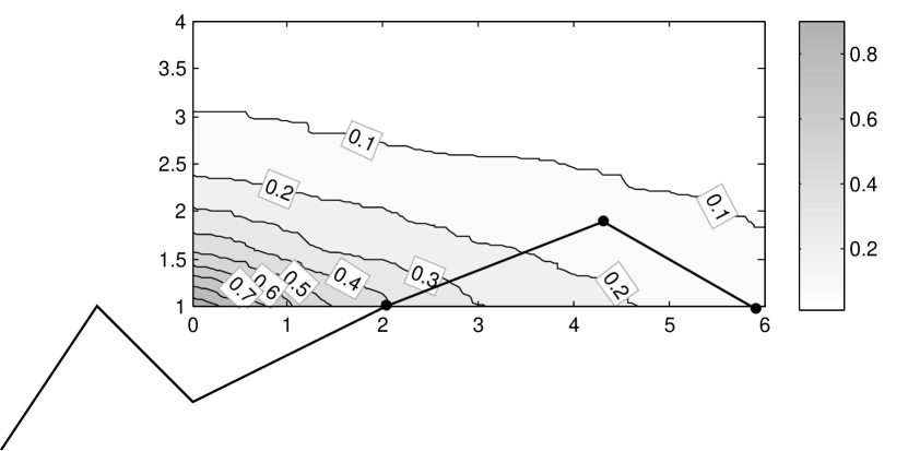
((a)) EUR-USD

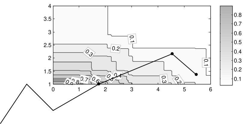
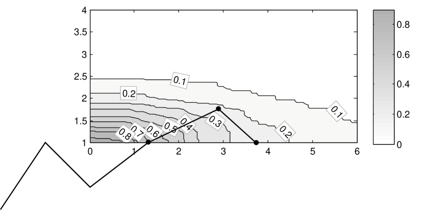
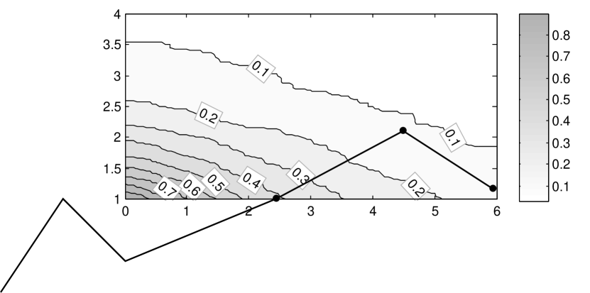
((b)) DAX-Future

Figure 12: The reversed cumulative distribution function $\tilde{F}(x,y)$ from (3) is plotted and the expectations from (4), (5) and  (6) are marked. The aggregation is 1 day, 1 hour and 10 minutes from top to bottom.

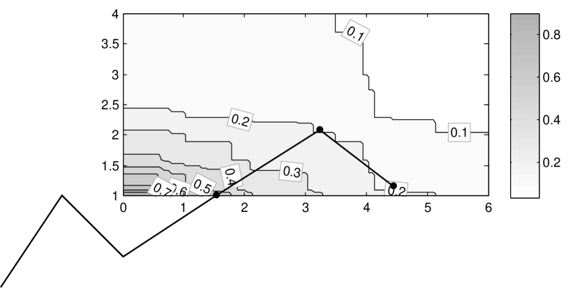
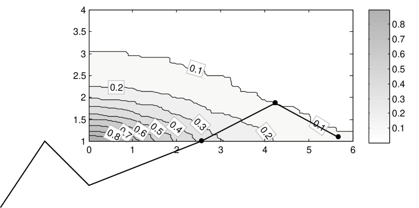
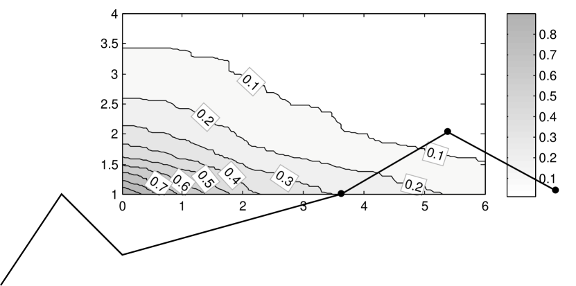
((a)) Gold

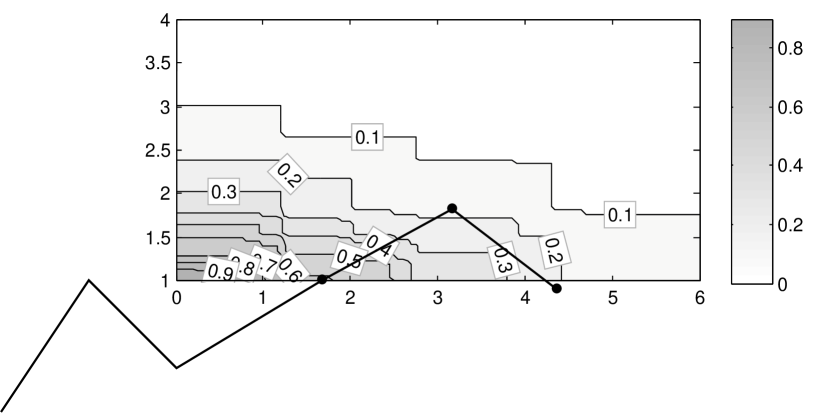
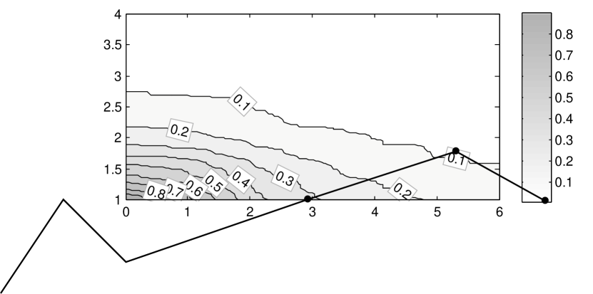
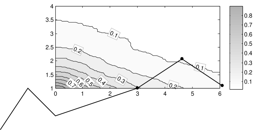
((b)) Crude Oil

Figure 13: The reversed cumulative distribution function $\tilde{F}(x,y)$ from (3) is plotted and the expectations from (4), (5) and  (6) are marked. The aggregation is 1 day, 1 hour and 10 minutes from top to bottom.

4 Conclusions

To identify a trend the strict trend definition from Dow has been used. The relevant extrema of the chart were found by the MinMax algorithm of [9] with the MACD as SAR process. Except for the timescale we always used the default parameter settings and did not need any optimization. We only set the timescale appropriate to match the dominant wavelength, which we obtained from the time shift with the highest autocorrelation of the price chart. We then saw many different results for trends on four different underlyings. One important observation is that the movement phase is relatively slow in comparison with the correction. We also see some side effects from the efficient-market hypothesis: We saw that the gain $G_{\textnormal{1--2--3,\%}}$ and $G_{\textnormal{3--2--3,\%}}$ is roughly at 50% and the probability of getting this gain, i.e. of reaching the last P2, is also about 50%. Improvements of these results could be appropriate selections of high potential situations. This could be done by filters and the use of nested trends.

References

- [1] Appel, Gerald: Technical Analysis: Power Tools for Active Investors. Financial Times Prentice Hall, Upper Saddle River, New Jersey, 2005.
- [2] Cene, E.: Professioneller Börsenhandel. FinanzBuch Verlag, München, 2011.
- [3] Chande, T. S. \btxandlong S. Kroll: The New Technical Trader. John Wiley & Sons, Hoboken, 1994.
- [4] Dürschner, M. G.: Technische Analyse mit EMD. Wiley, Hoboken, New Jersey, 2013.
- [5] Fama, E. F. \btxandlong M. E. Blume: Filter Rules and Stock-Market Trading. Journal of Business, 39:226–241, 1966.
- [6] Heckmann, T.: Markttechnische Handelssysteme, quantitative Kursmuster und saisonale Kursanomalien. Eul Verlag, Lohmar, 2009.
- [7] Huang, N. E., Z. Shen, S. R. Long, M. C. Wu, H. H. Shih, Q. Zheng, N.-C. Yen, C. C. Tung \btxandlong H. H. Liu: The empirical mode decomposition and the Hilbert spectrum for nonlinear and non-stationary time series analysis. Proceedings of the Royal Society of London, 454(1971):903–995, 1998.
- [8] Leuthold, R. M.: Random walk and price trends: The live cattle futures market. The Journal of Finance, 27(4):879–889, 1972.
- [9] Maier-Paape, S.: Automatic One Two Three. Quantitative Finance, 2013.
- [10] Meyberg, K. \btxandlong P. Vachenauer: Höhere Mathematik 2. Springer, Heidelberg, 2006.
- [11] Mittelhammer, R. C.: Mathematical Statistics for Economics and Business. Springer, Heidelberg, 1999.
- [12] Poulos, E. M.: Of Trends and Random Walks. Technical analysis of Stocks & Commodities, 9(2):49–52, 1991.
- [13] Sidney, S. A.: Price Movements in speculative Markets: Trends or Random Walks. Industrial Management Review Industrial Management Review, 2:7–26, 1961.
- [14] Voigt, M.: Das große Buch der Markttechnik. FinanzBuch Verlag, München, 7. \btxeditionlong, 2010.
- [15] Wilder, W. J.: New Concepts in Technical Trading Systems. Trend Research, McLeansville, North Carolina, 1978.