A Bayesian model for recognizing handwritten mathematical expressions

Abstract

Recognizing handwritten mathematics is a challenging classification problem, requiring simultaneous identification of all the symbols comprising an input as well as the complex two-dimensional relationships between symbols and subexpressions. Because of the ambiguity present in handwritten input, it is often unrealistic to hope for consistently perfect recognition accuracy. We present a system which captures all recognizable interpretations of the input and organizes them in a parse forest from which individual parse trees may be extracted and reported. If the top-ranked interpretation is incorrect, the user may request alternates and select the recognition result they desire. The tree extraction step uses a novel probabilistic tree scoring strategy in which a Bayesian network is constructed based on the structure of the input, and each joint variable assignment corresponds to a different parse tree. Parse trees are then reported in order of decreasing probability. Two accuracy evaluations demonstrate that the resulting recognition system is more accurate than previous versions (which used non-probabilistic methods) and other academic math recognizers.

1 Introduction

Many software packages exist which operate on mathematical expressions. Such software is generally produced for one of two purposes: either to create two-dimensional renderings of mathematical expressions for printing or on-screen display (e.g., LaTeX, MathML), or to perform mathematical operations on the expressions (e.g., Maple, Mathematica, Sage, and various numeric and symbolic calculators). In both cases, the mathematical expressions themselves must be entered by the user in a linearized, textual format specific to each software package.

This method of inputting math expressions is unsatisfactory for two main reasons. First, it requires users to learn a different syntax for each software package they use. Second, the linearized text formats obscure the two-dimensional structure that is present in the typical way users draw math expressions on paper. This is demonstrated with some absurdity by software designed to render math expressions, for which one must linearize a two-dimensional expression and input it as a text string, only to have the software re-create and display the expression’s original two-dimensional structure.

Mathematical software is typically used as a means to accomplish a particular goal that the user has in mind, whether it is creating a web site with mathematical content, calculating a sum, or integrating a complex expression. The requirement to input math expressions in a unique, unnatural format is therefore an obstacle that must be overcome, not something learned for its own sake. As such, it is desirable for users to input mathematics by drawing expressions in two dimensions as they do with pen and paper.

Academic interest in the problem of recognizing hand-drawn math expressions originated with Anderson’s doctoral research in the late 1960’s [2]. Interest has waxed and waned in the intervening decades, and recent years have witnessed renewed attention to the topic, potentially spurred on by the nascent Competition on Recognition of Handwritten Mathematical Expressions (CROHME) [11, 12].

However, math expressions have proved difficult to recognize effectively. Even the best state of the art systems (as measured by CROHME) are not sufficiently accurate for everyday use by non-specialists. The recognition problem is complex as it requires not only symbols to be recognized, but also arrangements of symbols, and the semantic content that those arrangements represent. Matters are further complicated by the large symbol set and the ambiguous nature of both handwritten input and mathematical syntax.

1.1 MathBrush

Our work is done in the context of the MathBrush pen-based math system [5]. Using MathBrush, one draws an expression, which is recognized incrementally as it is drawn (Fig. 1a). At any point, the user may correct erroneous recognition results by selecting part or all of the expression and choosing an alternative recognition from a drop-down list (Fig. 1b). Once the expression is completely recognized, it is embedded into a worksheet interface through which the user may manipulate and work with the expression via computer algebra system commands (Fig. 1c).

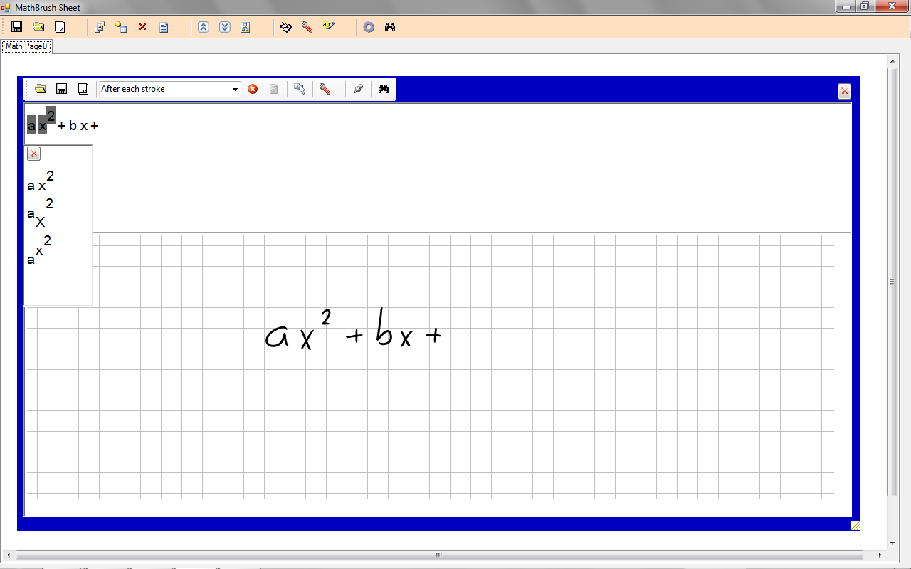
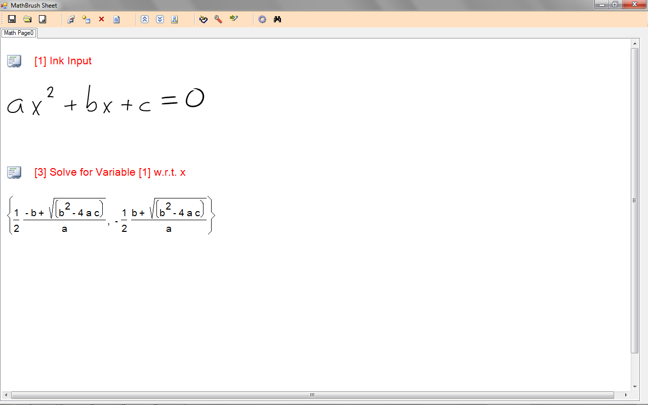
Figure 1: MathBrush. From top to bottom: (a) input interface, (b) correction drop-down, (c) worksheet interface.

For our purposes, the crucial element of this description is that the user may at any point request alternative interpretations of any portion of their input. This behaviour differs from that of most other recognition systems, which present the user with a single, potentially incorrect result. We instead acknowledge the fact that recognition will not be perfect all of the time, and endeavour to make the correction process as fast and simple as possible. Much of our work is motivated by the necessity of maintaining multiple interpretations of the input so that lists of alternative recognition results can be populated if the need arises.

We have previously reported techniques for capturing and reporting these multiple interpretations [9], and some of those ideas remain the foundation of the work presented in this paper. In particular, the two-dimensional syntax of mathematics is organized and understood through the formalism of relational context-free grammars (RCFGs), a multi-dimensional generalization of traditional context-free grammars. It is necessary to place restrictions on the structure of the input so that parsing with RCFGs takes a reasonable amount of time, but once this is done it is fairly straightforward to adapt existing parsing algorithms to RCFGs so that they produce a data structure called a parse forest which simultaneously represents all recognizable interpretations of an input. The parse forest is the primary tool we use to organize alternative recognition results in case the user desires to see them. When it does become necessary to populate drop-down lists in MathBrush with recognition results, individual parse trees – each representing a different interpretation of the input – must be extracted from the parse forest. As with parsing, some restrictions are necessary in this step to achieve reasonable performance.

Our previous work formalized the notion of ambiguity in terms of fuzzy sets and represented portions of the input as fuzzy sets of math expressions. In this paper, we abandon the language of fuzzy sets, develop a more general notion of how recognition processes interact with the grammar model, and introduce a Bayesian scoring model for parse trees. The scoring model incorporates results from recognition systems as well as “common-sense” knowledge drawn from training corpora. The recognition systems contributing to the model include a novel stroke grouping system, a combination symbol classifier based on quantile-mapped distance functions, and a naive Bayesian relation classifier. An algebraic technique eliminates many model variables from tree probability calculations, yielding an efficiently computable probability function. The resulting recognition system is significantly more accurate than other academic math recognizers, including the fuzzy variant we used previously.

The rest of this paper is organized as follows. Section 2 summarizes some recent probabilistic approaches to the math recognition problem and points out some of the issues that arise in practice when applying standard probabilistic models to this problem. Section 3 summarizes the theory and algorithms behind our RCFG variant, describing how to construct and extract trees from a parse forest for a given input. This section also states the restrictions and assumptions we use to attain reasonable recognition speeds. Section 4 is devoted to the new probabilistic tree scoring function we have devised for MathBrush, based on constructing a Bayesian network for a given input. Finally, Section 5 replicates the 2011 and 2012 CROHME accuracy evaluations, demonstrating the effectiveness of the probabilistic scoring framework, and Section 6 concludes the paper with a summary and some promising directions for future research.

2 Existing research

There is a significant and expanding literature concerning the math recognition problem. Many recent systems and approaches are summarized in the CROHME reports [11, 12]. We will comment directly on a few recent approaches using probabilistic methods.

2.1 Alvaro et al

The system developed by Alvaro et al [1] placed first in the CROHME 2011 recognition contest [11]. It is based on earlier work of Yamamoto et al [18]. A grammar models the formal structure of math expressions. Symbols and the relations between them are modeled stochastically using manually-defined probability functions. The symbol recognition probabilities are used to seed a parsing table on which a CYK-style parsing algorithm proceeds to obtain an expression tree representing the entire input.

In this scheme, writing is considered to be a generative stochastic process governed by the grammar rules and probability distributions. That is, one stochastically generates a bounding box for the entire expression, chooses a grammar rule to apply, and stochastically generates bounding boxes for each of the rule’s RHS elements according to the relation distribution. This process continues recursively until a grammar rule producing a terminal symbol is selected, at which point a stroke (or, more properly, a collection of stroke features) is stochastically generated.

Given a particular set of input strokes, Alvaro et al find the sequence of stochastic choices most likely to have generated the input. However, stochastic grammars are known to biased toward short parse trees (those containing few derivation steps) [10]. In our own experiments with such approaches, we encountered difficulties in particular with recognizing multi-stroke symbols in the context of full expressions. The model has no intrinsic notion of symbol segmentation, and the bias toward short parse trees caused the recognizer to consistently report symbols with many strokes even when they had poor recognition scores. Yet to introduce symbol segmentation scores in a straightforward way causes probability distributions to no longer sum to one. Alvaro et al allude to similar difficulties when they mention that their symbol recognition probabilities had to be rescaled to account for multi-stroke symbols.

In Section 4, we propose a different solution. We abandon the generative model in favour of one that explicitly reflects the stroke-based nature of the input, and furthermore include a nil value to account for groups of strokes that are not, in fact, symbols.

2.2 Awal et al

While the system described by Awal et al [3] was included in the CROHME 2011 contest, its developers were directly associated with the contest and were thus not official participants. However, their system scored higher than the winning system of Alvaro et al, so it is worthwhile to examine its construction.

A dynamic programming algorithm first proposes likely groupings of strokes into symbols, although it is not clear what cost function the dynamic program is minimizing. Each of the symbol groups is recognized using neural networks whose outputs are converted into a probability distribution over symbol classes.

Math expression structure is modeled by a context-free grammar in which each rule is linear in either the horizontal of vertical direction. Spatial relationships between symbols and subexpressions are modeled as two independent Gaussians on position and size difference between subexpression bounding boxes. These probabilities along with those from symbol recognition are treated as independent variables, and the parse tree minimizing a cost function defined in terms of weighted negative log likelihoods is reported as the final parse.

This method as a whole is not probabilistic as the variables are not combined in a coherent model. Instead, probability distributions are used as components of a scoring function. This pattern is common in the math recognition literature: distribution functions are used when they are useful, but the overall strategy remains ad hoc. Vestiges of this may be seen in our own work throughout Section 4; however in this paper we take the next step and re-combine scoring functions into a coherent probabilistic model.

2.3 Shi, Li, and Soong

Working with Microsoft Research Asia, Shi, Li, and Soong proposed a unified HMM-based method for recognizing math expressions [14]. Treating the input strokes as a temporally-ordered sequence, they use dynamic programming to determine the most likely points at which to split the sequence into distinct symbol groups, the most likely symbols each of those groups represent, and the most likely spatial relation between temporally-adjacent symbols. Some local context is taken into account by treating symbol and relation sequences as Markov chains. This process results in a DAG, which may be easily converted to an expression tree.

To compute symbol likelihoods, a grid-based method measuring point density and stroke direction is used to obtain a feature vector. These vectors are assumed to be generated by a mixture of Gaussians with one component for each known symbol type. Relation likelihoods are also treated as Gaussian mixtures of extracted bounding-box features. Group likelihoods are computed by manually-defined probability functions.

This approach is elegant in its unity of symbol, relation, and expression recognition. The reduction of the input to a linear sequence of strokes dramatically simplifies the parsing problem. But this assumption of linearity comes at the expense of generality. The HMM structure strictly requires strokes to be drawn in a pre-determined linear sequence. That is, the model accounts for ambiguity in symbol and relation identities, but not for the two-dimensional structure of mathematics. As such, the method is unsuitable for applications such as MathBrush, in which the user may draw, erase, move, or otherwise edit any part of their input at any time.

3 Relational grammars and parsing

Relational grammars are the primary means by which the MathBrush recognizer associates mathematical semantics with portions of the input. We previously described a fuzzy relational grammar formalism which explicitly modeled recognition as a process by which an observed, ambiguous input is interpreted as a certain, structured expression [9]. In this work, we define the grammar slightly more abstractly so that it has no intrinsic tie to fuzzy sets and may be used with a variety of scoring functions. Interested readers are referred to [9] and [7] for more details.

3.1 Grammar definition and terminology

Relational context-free grammars are defined as follows.

Definition 1.

A relational context-free grammar $G$ is a tuple $\left(\Sigma,N,S,O,R,P\right)$, where

• $\Sigma$ is a set of terminal symbols,

• $N$ is a set of non-terminal symbols,

• $S\in N$ is the start symbol,

• $O$ is a set of observables,

• $R$ is a set of relations on $I$, the set of interpretations of $G$ (described below),

• $P$ is a set of productions, each of the form $A_{0}\overset{r}{\Rightarrow}A_{1}A_{2}\cdots A_{k}$, where $A_{0}\in N,r\in R$, and $A_{1},\ldots,A_{k}\in N\cup\Sigma$,

The basic elements of a CFG are present in this definition as $\Sigma,N,S,$ and $P$, though the form of an RCFG production is slightly more complex than that of a CFG production. However, there are several less familiar components as well.

3.1.1 Observables, Expressions and interpretations

The set $O$ of observables is the set of all possible inputs – in our case each observable is a set of ink strokes, and each ink stroke is an ordered sequence of points in $\mathbb{R}^{2}$.

An expression is the generalization of a string to the RCFG case. The form of an expression reflects the relational form of the grammar productions. Any terminal symbol $\alpha\in\Sigma$ is a terminal expression. An expression $e$ may also be formed by concatenating several expressions $e_{1},\ldots,e_{k}$ by a relation $r\in R$. Such an $r$-concatenation is written $e_{1}r\cdots re_{k}$.

The representable set of $G$, written $\mathcal{L}(G)$, is the set of all expressions formally derivable using the nonterminal, terminals, and productions of a grammar $G$. $\mathcal{L}(G)$ generalizes the notion of the language generated by a grammar to RCFGs.

An interpretation, then, is a pair $(e,o)$, where $e\in\mathcal{L}(G)$ is a representable expression and $o$ is an observable.This definition links the formal structure of the grammar with the geometric structure of the input – an interpretation is essentially a parse of $o$ where the structure of $e$ encodes the hierarchical structure of the parse. The set of interpretations $I$ referenced in the RCFG definition is just the set of all possible interpretations:

$$I=\left\{\left(e,o\right):e\in\mathcal{L}(G),o\in O\right\}.$$

In our previous work with fuzzy sets, the set of interpretations was fuzzy. This required a scoring model to be embedded into the grammar’s structure and added otherwise unnecessary components to the grammar definition. The present formalism is slightly more abstract. It loses no expressive power but leaves scoring models and data organization as implementation details, rather than as fundamental grammar components.

3.1.2 Relations and productions

The relations in $R$ model the spatial relationships between subexpressions. In mathematics, these relationships often determine the semantic interpretation of an expression (e.g., $a$ and $x$ written side-by-side as $ax$ means something quite different from the diagonal arrangement $a^{x}$). An important feature of these grammar relations is that they act on interpretations – pairs of expressions and observables. This enables relation classifiers to use knowledge about how particular expressions or symbols fit together when interpreting geometric features of observables. By doing so, an expression like the one shown in Figure 2 may be interpreted as either $P^{x+a}$ or $px+a$ depending on the identity of its symbols.

Figure 2: An expression in which the optimal relation depends on symbol identity.

We use five relations, denoted $\rightarrow\,,\nearrow\,,\searrow\,,\downarrow\,,\odot\,$. The four arrows indicate the general writing direction between two subexpressions, and $\odot\,$ indicates containment notation, as used in square roots.

The productions in $P$ are similar to context-free grammar productions. The relation $r$ appearing above the production symbol ($\overset{r}{\Rightarrow}$) indicates that $r$ must be satisfied by adjacent elements of the RHS. Formally, given a production $A_{0}\overset{r}{\Rightarrow}A_{1}A_{2}\cdots A_{k}$, if $o_{i}$ ($i=1,\ldots,k$) denotes an observable interpretable as an expression $e_{i}$, and each $e_{i}$ is itself derivable from a nonterminal $A_{i}$, then for the observable $o_{1}\cup\cdots\cup o_{k}$ to be interpretable as the $r$-concatenation $e_{1}r\cdots re_{k}$ requires that $\left(\left(e_{i},o_{i}\right),\left(e_{i+1},o_{i+1}\right)\right)\in r$ for $i=1,\ldots,k-1$. That is, all adjacent pairs of sub-interpretations must satisfy the grammar relation for them to be combinable into a larger interpretation.

For example, consider the following toy grammar:

[EXPR] $$\overset{}{\Rightarrow}\mbox{{\tt[ADD]}}\mid\mbox{{\tt[TERM]}}$$

[ADD] $$\overset{\rightarrow\,}{\Rightarrow}\mbox{{\tt[TERM]}}+\mbox{{\tt[EXPR]}}$$

[TERM] $$\overset{}{\Rightarrow}\mbox{{\tt[MULT]}}\mid\mbox{{\tt[LEAD-TERM]}}$$

[LEAD-TERM] $$\overset{}{\Rightarrow}\mbox{{\tt[SUP]}}\mid\mbox{{\tt[FRAC]}}\mid\mbox{{\tt[SYM]}}$$

[MULT] $$\overset{\rightarrow\,}{\Rightarrow}\mbox{{\tt[LEAD-TERM]}}\mbox{{\tt[TERM]}}$$

[FRAC] $$\overset{\downarrow\,}{\Rightarrow}\mbox{{\tt[EXPR]}}\text{---}\mbox{{\tt[EXPR]}}$$

[SUP] $$\overset{\nearrow\,}{\Rightarrow}\mbox{{\tt[SYM]}}\mbox{{\tt[EXPR]}}$$

[SYM] $$\overset{}{\Rightarrow}\mbox{{\tt[VAR]}}\mid\mbox{{\tt[NUM]}}$$

[VAR] $$\overset{}{\Rightarrow}a\mid b\mid\cdots\mid z$$

[NUM] $$\overset{}{\Rightarrow}0\mid 1\mid\cdots\mid 9$$

In this example, the production for [ADD] models the syntax for infix addition: two expressions joined by the addition symbol, written from left to right. The production for [FRAC] has a similar structure – two expressions joined by the fraction bar symbol – but specifies that its components should be organized from top to bottom using the $\downarrow\,$ relation. The production for [MULT] illustrates the ease with which different relations and writing directions may be combined together to form larger expressions. The [LEAD-TERM] term may be a superscript (using the $\nearrow\,$ relation), a fraction (using the $\downarrow\,$ relation), or a symbol, but no matter which of those subexpressions appears as the leading term, it must satisfy the left-to-right relation $\rightarrow\,$ when combined with the training term.

3.2 Parsing with Unger’s method

Compared with traditional CFGs, there are two main sources of ambiguity and difficulty when parsing RCFGs: the symbols in the input are unknown, both in the sense of what parts of the input constitute a symbol, and what the identity of each symbol is; and because the input is two-dimensional, there is no straightforward linear order in which to traverse the input strokes. Additionally, there may be ambiguity arising from relation classification uncertainty: we may not know for certain which grammar relation links two subexpressions together.

We manage and organize these sources of uncertainty by using a data structure called a parse forest to simultaneously represent all recognizable parses of the input. A parse forest is a graphical structure in which each node represents all of the parses of a particular subset of the input using a particular grammar nonterminal or production. There are two types of nodes:

1. OR nodes. Each of an OR node’s parse trees is taken directly from one of the node’s children. There are two types of OR nodes:

   1. Nonterminal nodes of the form $(A,o)$, representing the parses of a nonterminal $A$ on a subset $o$ of the input. The parse tree of $A$ on $o$ is just the parse tree of some production with LHS $A$ on $o$.

   2. Production nodes of the form $(p,o)$, representing the parses of a production $p$ of the form $A_{0}\overset{r}{\Rightarrow}A_{1}\cdots A_{k}$ on a subset $o$ of the input. Each such parse tree arises by parsing $p$ on some partition of $o$ into $k$ subsets.

2. AND nodes. Each of an AND node’s parse trees is an $r$-concatenation to which each of the node’s children contributes one subexpression. AND nodes have the form $(p;(o_{1},\ldots,o_{k}))$, representing the parses of a production $p$ of the form above on a partition $o_{1},\ldots,o_{k}$ of some subset $o_{1}\cup\cdots\cup o_{k}$ of the input. Each subexpression $e_{i}$ is itself a parse of $A_{i}$ on the partition subset $o_{i}$.

Parsing an RCFG may be divided into two steps: forest construction, in which a shared parse forest is created that represents all recognizable parses of the input, and tree extraction, in which individual parse trees are extracted from the forest in decreasing order of tree score.

3.2.1 Restricting feasible partitions

To obtain reasonable performance when parsing with RCFGs, it is necessary to restrict the ways in which input observables may be partitioned and recombined (otherwise, partitions of the input using all $2^{n}$ subsets would need to be considered). We choose to restrict partitions to horizontal and vertical concatenations, as follows.

Each of the five grammar relations is associated with either the $x$ direction of $y$ direction ($\rightarrow\,,\nearrow\,,\odot\,$ with $x$, $\searrow\,,\downarrow\,$ with $y$). Then when parsing an observable $o$ using a production $A_{0}\overset{r}{\Rightarrow}A_{1}\cdots A_{k}$, $o$ is partitioned by either horizontal or vertical cuts based on the directionality of the relation $r$. For example, when parsing the production $\mbox{{\tt[ADD]}}\overset{\rightarrow\,}{\Rightarrow}\mbox{{\tt[TERM]}}+\mbox{{\tt[EXPR]}}$ on the input from Figure 2, we would note that the relation $\rightarrow\,$ requires horizontal concatenations, and so split the input into three horizontally-concatenated subsets using two vertical cuts. In general, there are $\binom{n}{k-1}$ ways to partition $n$ input strokes into $k$ concatenated subsets.

The restriction to horizontal and vertical concatenations is quite severe, but it reduces the worst-case number of subsets of the input which may need to be considered during parsing from $2^{n}$ to $\mathcal{O}(n^{4})$. Furthermore, the restriction effectively linearizes the input in either the $x$ or $y$ dimension, depending on which grammar relation is being considered. This linearity is sufficiently similar to the implicit linearity of traditional CFG parsing that one may adapt CFG parsing algorithms to the relational grammar case without much difficulty.

3.2.2 Unger’s method

Unger’s method is a fairly brute-force algorithm for parsing CFGs [17]. It is easily extended to become a tabular RCFG parser as follows.

First, the grammar is re-written so that each production is either terminal (of the form $A_{0}\overset{}{\Rightarrow}\alpha$, where $\alpha\in\Sigma$), or nonterminal (of the form $A_{0}\overset{r}{\Rightarrow}A_{1}\cdots A_{k}$, where each $A_{i}\in N$), so there is no mixing of terminal and non-terminal symbols within productions. Then our variant of Unger’s method constructs a parse forest by recursively applying the following rules, where $p$ is a production and $o$ is an input observable:

1. If $p$ is a terminal production, $A_{0}\overset{}{\Rightarrow}\alpha$, then check if $o$ is recognizable as $\alpha$ according to a symbol recognizer. If it is, then add the interpretation $(o,\alpha)$ to table entry $(o,\alpha)$; otherwise parsing fails.

2. Otherwise, $p$ is of the form $A_{0}\overset{r}{\Rightarrow}A_{1}\cdots A_{k}$. For every relevant partition $o$ into subsets $o_{1},\ldots,o_{k}$ (either a horizontal or vertical concatenation, as appropriate), parse each nonterminal $A_{i}$ on $o_{i}$. If all of the sub-parses succeed, then add $\left(p;(o_{1},\ldots,o_{k})\right)$ to table entry $(o,A_{0})$.

Naively, $\mathcal{O}(|o|^{k-1})$ partitions must be considered in step 2. But since Unger’s method explicitly enumerates these partitions, we may easily optimize the algorithm by restricting which partitions are explored, thereby avoiding the recursive part of step 2 when possible. In bottom-up algorithms like CYK or Earley’s method, such optimizations are not possible (or are at least much more difficult to implement) because the subdivision of the input into subexpressions is determined implicitly from the bottom up.

The output of this variant of Unger’s method is a parse forest containing every parse of the input which could be recognized. The next step is to extract individual parse trees from the parse forest in decreasing score order. The first, highest-scoring tree is presented to the user as they are writing (see Figure 1a). If the user selects a portion of the expression and requests alternative recognition results, then further parse trees are extracted and displayed in the drop-down lists.

3.3 Parse tree extraction

To find a parse tree of the entire input observable $o$, we need only start at the root node $(S,o)$ of the parse forest ($S$ being the grammar’s start symbol) and, whenever we are at an OR node, follow the link to one of the node’s children. Whenever we are at an AND node, follow the links to all of the node’s children simultaneously. Once all branches of such a path reach terminal expressions, we have found a parse tree. Moreover, any combination of choices at OR nodes that yields such a branching path gives a valid parse tree.

The problem, then, is how to enumerate those paths in such a way that the most reasonable parse is found first, then the next most reasonable, and so on. Our approach is to equip each of the nodes in the parse forest with a priority queue ordered by parse tree score. Tree extraction is then treated as an iteration problem. Initially, we insert the highest-scoring parse tree of a node into the node’s priority queue. Then, whenever a tree is required from that node, it is obtained by popping the highest-scoring tree from the queue. The queue is then prepared for subsequent iteration by pushing in some more trees in such a way that the next-highest-scoring tree is guaranteed to be present.

More specifically, to find the highest-scoring tree at an OR node $N$, we recursively find the highest-scoring trees at all of the node’s children and add them to the queue. Then the highest-scoring tree at $N$ is just the highest-scoring tree out of those options. When a tree is popped from the priority queue, it was obtained from a child node of $N$ (call it $C$) as, say, the $i$th highest-scoring tree at $C$. To prepare for the next iteration step, we obtain the $i+1$st highest-scoring tree at $C$ and add that into the priority queue of $N$.

To find the highest-scoring tree at an AND node $N$ representing parses of $A_{0}\overset{r}{\Rightarrow}A_{1}\cdots A_{k}$ on a partition $o_{1},\ldots,o_{k}$, we again recursively find the highest-scoring parses of the node’s children – in this case the OR nodes $(A_{1},o_{1}),\ldots,(A_{k},o_{k})$. Calling these expressions $e_{1},\ldots,e_{k}$, the $r$-concatenation $e_{1}r\cdots re_{k}$ is the highest-scoring tree at $N$. Now, any $r$-concatenation obtained from the $k$ child nodes of $N$ can be represented by a $k$-tuple $(n_{1},\ldots,n_{k})$, where each $n_{i}$ indicates the rank of $e_{i}$ in the iteration over trees from node $(A_{i},o_{i})$. (The first, highest-scoring tree has rank 1, the second-highest-scoring tree has rank 2, etc.) The first tree is therefore represented by the tuple $(1,1,\ldots,1)$. Whenever we report a tree from node $N$, we prepare for the next iteration step by examining the tuple $(n_{1},\ldots,n_{k})$ corresponding to the tree just reported, creating $k$ parse trees corresponding to the tuples $(n_{1}+1,n_{2},\ldots,n_{k}),(n_{1},n_{2}+1,\ldots,n_{k}),\ldots,(n_{1},\ldots,n_{k-1},n_{k}+1)$ by requesting the relevant subexpression trees from the child nodes of $N$, and pushing those $k$ trees into the priority queue of $N$.

These procedures for obtaining the best and next-best parse trees at OR- and AND-nodes are similar to those we described previously [9]. In that description, we required the implementation of the grammar relations to satisfy certain properties in order for the tree exraction algorithms to succeed. Here, similarly to the grammar definition, we reformulate our assumptions more abstractly to promote independence between theory and implementation.

The tree extraction algorithm is guaranteed to enumerate parse trees in strictly decreasing order of any parse-tree scoring function $\operatorname{sc}(e,o)$ (for $e$ an expression and $o$ an observable) that satisfies the following assumptions. In the assumptions, $S(\alpha,o)$ is a symbol recognition score for recognizing the observable $o$ as the terminal symbol $\alpha$, $G(o)$ is a stroke grouping score indicating the extent to which an observable $o$ is considered to be a symbol, and $R_{r}((e_{1},o_{1}),(e_{2},o_{2}))$ is a relation score indicating the extent to which the grammar relation $r$ is satisfied between the interpretations $(e_{1},o_{1})$ and $(e_{2},o_{2})$. Larger values of these scoring functions indicate higher recognition confidence.

1. The score of a terminal interpretation $(\alpha,t)$ is some function $g$ of the symbol and grouping scores,

   $$\operatorname{sc}(\alpha,t)=g(S(\alpha,t),G(t)),$$

   and $g$ increases monotonically with $S(\alpha,o)$.

2. The score of a nonterminal interpretation $(e,t)=(e_{1}r\cdots re_{k},(t_{1},\ldots,t_{k}))$ is some function $f_{k}$ of the sub-interpretation scores and the relation scores between adjacent sub-interpretations,

   $$\operatorname{sc}(e,t)=f_{k}( \operatorname{sc}(e_{1},t_{1}),\ldots,\operatorname{sc}(e_{k},t_{k}),$$

   $$R_{r}((e_{1},t_{1}),(e_{2},t_{2})),\ldots,R_{r}((e_{k-1},t_{k-1}),(e_{k},t_{k}))).$$

   and $f_{k}$ increases monotonically with all of its parameters.

These assumptions admit a number of reasonable underlying scoring and combination functions. The next section will develop concrete scoring functions based on Bayesian probability theory and some underlying low-level classification techniques.

4 A Bayesian scoring function

At a high level, the scoring function $\operatorname{sc}(e,o)$ of an interpretation of some subset $o$ of the entire input $\hat{o}$ is organized as a Bayesian network which is constructed specifically for $\hat{o}$.

4.1 Model organization

Given an input observable $\hat{o}$, the Bayesian scoring model includes several families of variables:

• An expression variable $E_{o}\in\mathcal{L}(G)\cup\left\{\textsc{nil}\right\}$ for each $o\subseteq\hat{o}$, distributed over representable expressions. $E_{o}=\textsc{nil}$ indicates that the subset $o$ has no meaningful interpretation.

• A symbol variable $S_{o}\in\Sigma\cup\left\{\textsc{nil}\right\}$ for each $o\subseteq\hat{o}$ indicating what terminal symbol $o$ represents. $S_{o}=\textsc{nil}$ indicates that $o$ is not a symbol. ($o$ could be a larger subexpression, or could have $E_{o}=\textsc{nil}$ as well.)

• A relation variable $R_{o_{1},o_{2}}\in R\cup\left\{\textsc{nil}\right\}$ indicating which grammar relation joins the subsets $o_{1},o_{2}\subset\hat{o}$. $R_{o_{1},o_{2}}=\textsc{nil}$ indicates that the subsets are not directly connected by a relation.

• A vector of grouping-oriented features $g_{o}$ for each $o\subseteq\hat{o}$.

• A vector of symbol-oriented features $s_{o}$ for each $o\subseteq\hat{o}$.

• A vector of relation-oriented features $f_{o}$ for each $o\subset\hat{o}$.

• A “symbol-bag” variable $B_{o}$ distributed over $\Sigma\cup\{\textsc{nil}\}$ for each $o\subseteq\hat{o}$.

At any point in the parse tree extraction algorithm, a particular interpretation $(e,o)$ of a subset of the input is under consideration and must be scored. Each such interpretation corresponds to a joint assignment to all of these variables, so our task is to define the joint probability function

$$P\left(\bigwedge_{o\subseteq\hat{o}}E_{o},\bigwedge_{o\subseteq\hat{o}}S_{o},\bigwedge_{o_{1},o_{2}\subset\hat{o}}R_{o_{1},o_{2}},\bigwedge_{o\subseteq\hat{o}}g_{o},\bigwedge_{o\subseteq\hat{o}}s_{o},\bigwedge_{o\subset\hat{o}}f_{o},\bigwedge_{o\subseteq\hat{o}}B_{o}\right).$$

in such a way that it may be calculated quickly.

The fact that joint variable assignments arise from parse trees imposes severe constraints on which variables can simultaneously be assigned non-nil values. For example, if $E_{o}=\textsc{nil}$, then $S_{o}=\textsc{nil}$, and any $R_{o,\ast}$ or $R_{\ast,o}$ is also nil. Also, $E_{o}$ is a terminal expression iff $S_{o}\neq\textsc{nil}$. In general, only those variables representing meaningful subexpressions in the parse tree – or relationships between those subexpression – will be non-nil. In all valid assignments, $B_{o}=S_{o}$ for all $o$; however the distribution of $S_{o}$ reflects recognition, while that of $B_{o}$ reflects prior domain knowledge.

We take advantage of these constraints to achieve efficient calculation of the joint probability. First, we factor the joint distribution as a Bayesian network,

$$P\left(\bigwedge_{o\subseteq\hat{o}}E_{o},\bigwedge_{o\subseteq\hat{o}}S_{o},\bigwedge_{o_{1},o_{2}\subset\hat{o}}R_{o_{1},o_{2}},\bigwedge_{o\subseteq\hat{o}}g_{o},\bigwedge_{o\subseteq\hat{o}}s_{o},\bigwedge_{o\subset\hat{o}}f_{o},\bigwedge_{o\subset\hat{o}}B_{o}\right)$$

$$= \prod_{o^{\prime}\subset\hat{o}}P\left(E_{o^{\prime}}\mid\bigwedge_{o\subset o^{\prime}}E_{o},\bigwedge_{o\subseteq o^{\prime}}S_{o},\bigwedge_{o_{1},o_{2}\subset o^{\prime}}R_{o_{1},o_{2}},\bigwedge_{o\subseteq o^{\prime}}g_{o},\bigwedge_{o\subseteq o^{\prime}}s_{o},\bigwedge_{o\subset o^{\prime}}f_{o}\right)$$

$$\times \prod_{o\subseteq\hat{o}}P\left(S_{o}\mid g_{o},s_{o}\right)$$

$$\times \prod_{o_{1},o_{2}\subset\hat{o}}P\left(R_{o_{1},o_{2}}\mid E_{o_{1}},E_{o_{2}},f_{o_{1}},f_{o_{2}}\right)$$

$$\times \prod_{o^{\prime}\subseteq\hat{o}}P\left(B_{o^{\prime}}\mid\bigwedge_{o\subseteq\hat{o}}S_{o}\right)$$

$$\times \prod_{o\subseteq\hat{o}}g_{o}\prod_{o\subseteq\hat{o}}s_{o}\prod_{o\subset\hat{o}}f_{o}.$$

Because of the number of variables, it is not feasible to compute this product directly. Instead, we remove the feature variables as they are functions only of the input, and factor out the product

$$Z=\prod_{o\subseteq\hat{o}}P\left(S_{o}=\textsc{nil}\mid g_{o},s_{o}\right)\times\prod_{o_{1},o_{2}\subset\hat{o}}P\left(R_{o_{1},o_{2}}=\textsc{nil}\mid E_{o_{1}},E_{o_{2}},f_{o_{1}},f_{o_{2}}\right).$$

This division leaves

$$P\left(\bigwedge_{o\subseteq\hat{o}}E_{o},\bigwedge_{o\subseteq\hat{o}}S_{o},\bigwedge_{o_{1},o_{2}\subset\hat{o}}R_{o_{1},o_{2}},\bigwedge_{o\subseteq\hat{o}}g_{o},\bigwedge_{o\subseteq\hat{o}}s_{o},\bigwedge_{o\subset\hat{o}}f_{o},\bigwedge_{o\in\hat{O}}B_{o}\right)$$

$$\propto \prod_{o^{\prime}\subset\hat{o},E_{o^{\prime}}\neq\textsc{nil}}P\left(E_{o^{\prime}}\mid\bigwedge_{o\subset o^{\prime}}E_{o},\bigwedge_{o\subseteq o^{\prime}}S_{o},\bigwedge_{o_{1},o_{2}\subset o^{\prime}}R_{o_{1},o_{2}},\bigwedge_{o\subseteq o^{\prime}}g_{o},\bigwedge_{o\subseteq o^{\prime}}s_{o},\bigwedge_{o\subset o^{\prime}}f_{o}\right)$$

$$\times \prod_{o\subseteq\hat{o},S_{o}\neq\textsc{nil}}\frac{P\left(S_{o}\mid g_{o},s_{o}\right)}{P\left(S_{o}=\textsc{nil}\mid g_{o},s_{o}\right)}$$

$$\times \prod_{o_{1},o_{2}\subset\hat{o},R_{o_{1},o_{2}}\neq\textsc{nil}}\frac{P\left(R_{o_{1},o_{2}}\mid E_{o_{1}},E_{o_{2}},f_{o_{1}},f_{o_{2}}\right)}{P\left(R_{o_{1},o_{2}}=\textsc{nil}\mid E_{o_{1}},E_{o_{2}},f_{o_{1}},f_{o_{2}}\right)}$$

$$\times \prod_{o^{\prime}\subset\hat{o}}P\left(B_{o^{\prime}}\mid\bigwedge_{o\subseteq\hat{o}}S_{o^{\prime}}\right).$$

Suppose our entire input observable contains $n$ strokes. Since the joint assignment to these variables originates with an interpretation – an expression $e$ along with an observable $o$ – at most $n$ symbol variables may be non-nil. An expression variable $E_{o}$ is only non-nil when $o$ is a subset of the input corresponding to a subexpression of $e$. A relation variable $R_{o_{1},o_{2}}$ is only non-nil when both $E_{o_{1}}$ and $E_{o_{2}}$ are non-nil and correspond to adjacent subexpressions of $e$. There are thus $\mathcal{O}(n)$ non-nil variables in any joint assignment, so the adjusted product may be calculated quickly. The RHS of the above expression is the scoring function used during parse tree extraction.

To meaningfully compare the scores of different parse trees, the constant of proportionality in this expression must be equal across all parse trees. Thus, the probabilities $P\left(S_{o}=\textsc{nil}\mid g_{o},s_{o}\right)$ and $P\left(R_{o_{1},o_{2}}=\textsc{nil}\mid E_{o_{1}},E_{o_{2}},f_{o_{1}},f_{o_{2}}\right)$ must be functions only of the input. To achieve this in practice, we fix $E_{o_{1}}=E_{o_{2}}=\textsc{gen}$ when computing $P\left(R_{o_{1},o_{2}}=\textsc{nil}\mid E_{o_{1}},E_{o_{2}},f_{o_{1}},f_{o_{2}}\right)$.

Dividing out $Z$ leaves four families of probability distributions which must be defined. We will consider each of them in turn.

4.2 Expression variables

The distribution of expression variables,

$$E_{o^{\prime}}\mid{\bigwedge_{o\subset o^{\prime}}E_{o},\bigwedge_{o\subseteq o^{\prime}}S_{o},\bigwedge_{o_{1},o_{2}\subset o^{\prime}}R_{o_{1},o_{2}},\bigwedge_{o\subseteq o^{\prime}}g_{o},\bigwedge_{o\subseteq o^{\prime}}s_{o},\bigwedge_{o\subset o^{\prime}}f_{o}},$$

is deterministic. In a valid joint assignment (i.e., one derived from a parse tree), each non-nil conditional expression variable $E_{o}$ is a subexpression of $E_{o^{\prime}}$, and the non-nil relation variables indicate how these subexpressions are joined together. This information completely determines what expression $E_{o^{\prime}}$ must be, so that expression is assigned probability 1.

4.3 Symbol variables

The distribution of symbol variables, ${S_{o}}\mid{g_{o},s_{o}}$, is based on the stroke grouping score $G(o)$ and the symbol recognition scores $S(\alpha,o)$ (These scores are described below.)

The nil probability of $S_{o}$ is allocated as

$$P\left(S_{o}=\textsc{nil}\mid g_{o},s_{o}\right)=1-\frac{N}{N+1},$$

where $N=\log(1+G(o)\max_{\alpha}\{S(\alpha,o)\})$, and the remaining probability mass is distributed proportionally to $S(o,\alpha)$:

$$P\left(S_{o}=\alpha\mid g_{o},s_{o}\right)\propto\frac{S(\alpha,o)}{\sum_{\beta\in\Sigma}S(\beta,o)}.$$

4.3.1 Stroke grouping score

The stroke grouping function $G(o)$ is based on intuitions about what characteristics of a group of strokes indicate that the strokes belong to the same symbol. These intuitions may be summarized by the following logical predicate using the variables defined in Table 1:

$$G=\left(D_{in}\vee\left(L_{in}\wedge\neg C_{in}\right)\right)\wedge\left(\neg L_{out}\vee C_{out}\right).$$

Name	Meaning
$G$	A group exists
$D_{in}$	Small distance between strokes within group
$L_{in}$	Large overlap of strokes within group
$C_{in}$	Containment notation used within group
$L_{out}$	Large overlap of group and non-group strokes
$C_{out}$	Containment notation used in group or overlapping non-group strokes

Table 1: Variables names for grouping predicate.

Using DeMorgan’s law, this predicate may be re-written as

$$G =\neg\left(\neg D_{in}\wedge\neg\left(L_{in}\wedge\neg C_{in}\right)\right)\wedge\neg\left(L_{out}\wedge\neg C_{out}\right)$$

$$=\neg\left(\neg D_{in}\wedge\neg X_{in}\right)\wedge\neg X_{out},$$

where $X_{\ast}=L_{\ast}\wedge\neg C_{\ast}$.

To make this approach quantitative, we measure several aspects of $o$, one for each of the RHS variables defined above:

• $d=\min\left\{\mbox{dist}(s^{\prime},s):s^{\prime}\in g\right\}$, where $\mbox{dist}(s_{1},s_{2})$ is the minimal distance between the curves traced by $s_{1}$ and $s_{2}$;

• $\ell_{in}=\operatorname{overlap}(g,s)$, where $\operatorname{overlap}(g,s)$ is the area of the intersection of the bounding boxes of $g$ and $s$ divided by the area of the smaller of the two boxes;

• $c_{in}=\max\left(C(s),\max\left\{C\left(s^{\prime}\right):s^{\prime}\in g\right\}\right)$, where $C\left(s\right)$ is the extent to which the stroke $s$ resembles a containment notation, as described below;

• $\ell_{out}=\max\left\{\operatorname{overlap}(g\cup\{s\},s^{\prime}):s^{\prime}\in S\setminus\left(g\cup\left\{s\right\}\right)\right\}$;

• $c_{out}=\max\left(c_{in},C\left(s^{\prime}\right)\right)$, where $s^{\prime}$ is the maximizer for $\ell_{out}$.

Together, these five measurements form the grouping-oriented feature vector $g_{o}$. The grouping function $G(o)$ is defined as a conditional probability:

$$G(o) =P\left(G\mid d,\ell_{in},c_{in},\ell_{out},c_{out}\right)$$

$$=\left(1-P\left(\neg D_{in}\mid d\right)P\left(\neg X_{in}\mid\ell_{in},c_{in}\right)\right)^{\beta}P\left(\neg X_{out}\mid\ell_{out},c_{in},c_{out}\right)^{1-\beta}$$

where we set

$$P\left(\neg D_{in}\mid d\right) =\left(1-e^{-d/\lambda}\right)^{\alpha}$$

$$P\left(\neg X_{in}\mid\ell_{in},c_{in}\right) =\left(1-\ell_{in}\left(1-c_{in}\right)\right)^{\left(1-\alpha\right)}$$

$$P\left(\neg X_{out}\mid\ell_{out},c_{out},c_{in}\right) =1-\ell_{out}\left(1-\max\left(c_{in},c_{out}\right)\right).$$

This definition is loosely based on treating the boolean variables from our logical predicate as random and independent. $\lambda$ is estimated from training data, while $\alpha,\beta$ were both fixed via experiments at $9/10$.

To account for containment notations in the calculation of $c_{in}$ and $c_{out}$, we annotate each symbol supported by the symbol recognizer with a flag indicating whether it is used to contain other symbols. (Currently only the $\sqrt{\phantom{x}}$ symbol has this flag set.) Then the symbol recognizer is invoked to measure how closely a stroke or group of strokes resembles a container symbol.

4.3.2 Symbol recognition score

The symbol recognition score $S(\alpha,o)$ for recognizing an input subset $o$ as a terminal symbol $\alpha$ uses a combination of four distance-based matching techniques within a template-matching scheme. In this scheme, the input strokes in $o$ are matched against model strokes taken from a stored training example of $\alpha$, yielding a match distance. This process is repeated for each of the training examples of $\alpha$, and the two smallest match distances are averaged for each technique, giving four minimal distances $d_{1},d_{2},d_{3},d_{4}$. The distances are then combined in a weighted sum

$$s_{\alpha}=\sum_{i=1}^{4}w_{i}Q_{i}(d_{i}),$$

where $Q_{i}:\mathbb{R}\rightarrow[0,1]$ is the quantile function for the distribution of values emitted by the $i$th technique. These quantiles are approximated by piecewise linear functions and serve to normalize the outputs of the various distance functions so that they may be meaningfully arithmetically combined. The weights are optimized from training data. Finally, $S(\alpha,o)=s_{\alpha}^{-2}$ so that small distances correspond to large scores. The symbol recognition feature vector $s_{o}$ in the Bayesian model contains the values $S(\alpha,o)$ for all terminals $\alpha$.

The four distance-based techniques used are as follows:

• A fast elastic matching variant [8] which finds a matching between the points of the input and model strokes and minimizes the sum of distances between matched points.

• A functional approximation technique [4] which models stroke coordinates as parametric functions expressed as truncated Legendre-Sobolev series. The match distance is the 2-norm between coefficient vectors.

• An offline technique [16] based on rasterizing strokes, treating filled pixels as points in Euclidean space, and computing the Hausdorff distance between those point sets.

• A feature-vector method using the 2-norm between vectors containing the following normalized measurements of the input and model strokes: bounding box position and size, first and last point coordinates, and total arclength.

4.4 Relation variables

The distribution of relation variables, $R_{o_{1},o_{2}}\mid{E_{o_{1}},E_{o_{2}},f_{o_{1}},f_{o_{2}}}$, is similar to the symbol variable case in that it is based on the output of a lower-level recognition method, with some of the probability mass being reserved for the nil assignment. In particular, let $R(r)$ denote the extent to which the observables $o_{1}$ and $o_{2}$ appear to satisfy the grammar relation $r$. Then we put

$$P\left(R_{o_{1},o_{2}}=\textsc{nil}\mid E_{o_{1}},E_{o_{2}},f_{o_{1}},f_{o_{2}}\right)=1-\frac{N}{N+1},$$

where $N=\log(1+\max_{r}R(r))$, and distribute the remaining probability mass proportionally to $R(r)$:

$$P\left(R_{o_{1},o_{2}}=r\mid E_{o_{1}},E_{o_{2}},f_{o_{1}},f_{o_{2}}\right)\propto\frac{R(r)}{\sum_{u\in R}R(u)}.$$

$R(r)$ is determined using two sources of information. The first is geometric information about the bounding boxes of $o_{1}$ and $o_{2}$. Let $\ell(o),r(o),t(o),$ and $b(o)$ respectively denote the left-, right-, top-, and bottom-most coordinates of an observable $o$. These four values form the relation-oriented feature vector $f_{o}$ in the Bayesian model. From two such vectors $f_{o_{1}}$ and $f_{o_{2}}$, the following relation classification features are obtained ($N$ is a normalization factor based on the sizes of $o_{1}$ and $o_{2}$):

$$f_{1} =\frac{\ell(o_{2})-\ell(S_{1})}{N}$$

$$f_{2} =\frac{r(o_{2})-r(o_{1})}{N}$$

$$f_{3} =\frac{\ell(o_{2})-r(o_{1})}{N}$$

$$f_{4} =\frac{b(o_{2})-b(o_{1})}{N}$$

$$f_{5} =\frac{t(o_{2})-t(o_{1})}{N}$$

$$f_{6} =\frac{t(o_{2})-b(o_{1})}{N}$$

$$f_{7} =\operatorname{overlap}(o_{1},o_{2})$$

The second type of information is prior knowledge about how two types of expressions are arranged when placed in each grammar relation. To represent this, each expression $e$ is associated with one or more relational classes by a function $\operatorname{c\ell}(e)$. Each terminal symbol is itself a relational class (e.g., $\int,x,+$). Several more classes represent symbol stereotypes, as summarized in Table 2. Finally, there are three generic classes: sym (any symbol), expr (any multi-symbol expression), and gen (for “generic”; any expression whatsoever).

Class name	Example symbols
Baseline	a c x
Ascender	2 A h
Descender	g y
Extender	( )
Centered	+ =
i	i
j	j
Large-Extender	$\int$
Root	$\sqrt{\phantom{x}}$
Horizontal	-
Punctuation	. , ’

Table 2: Relational class labels.

These labels are hierarchical with respect to specificity. For example, the symbol $c$ is also a baseline symbol, any baseline symbol is also a sym expression, and any sym expression is also a gen expression.

We construct a classed scoring function $R_{c_{1},c_{2}}$ for every pair $c_{1},c_{2}$ of classes. Then, to evaluate $R(r)$, we first try the most specific relevant classed scoring function. If, due to a lack of training data, it is unable to report a result, we fall back to a less-specific classed function. This process of gradually reducing the specificity of class labels continues until a score is obtained or both labels are the generic label gen.

Each of the classed scoring functions is a naive Bayesian model that treats each of the features $f_{i}$ as drawn from independent normally-distributed variables $F_{i}$. So

$$R_{c_{1},c_{2}}(r)=P\left(R=r\right)\prod_{i=1}^{7}P\left(F_{i}=f_{i}\mid R=r\right),$$

where $R$ is a categorical random variable distributed over the grammar relations. The parameters of these distributions are estimated from training data.

When calculating a product of the form above, we check whether the true mean of each distribution lies within a 95% confidence interval of the training data’s sample mean. If not, then the classed scoring function $R_{c_{1},c_{2}}(r)$ reports failure, and we fall back to less-specific relational class labels as described above.

4.5 “Symbol-bag” variables

The role of the symbol-bag variables $B_{o}$ is to apply a prior distribution to the terminal symbols appearing in the input, and to adapt that distribution based on which symbols are currently present. Because those symbols are not known with certainty, such adaptation may only be done imperfectly.

We collected symbol occurence and co-occurence rates from the Infty project corpus [15] as well as from the LaTeX  sources of University of Waterloo course notes for introductory algebra and calculus courses. The symbol occurence rate $r(\alpha)$ is the number of expressions in which the symbol $\alpha$ appeared and the co-occurence rate $c(\alpha,\beta)$ is the number of expressions containing both $\alpha$ and $\beta$.

In theory, each $B_{o}$ variable is identically distributed and satisfies

$$P\left(B_{o}=\textsc{nil}\mid S_{o}=\textsc{nil},\bigwedge_{o^{\prime}\subseteq\hat{o}}S_{o^{\prime}}\right)=1$$

and

$$P\left(B_{o}=\alpha\mid S_{o}=\delta,\bigwedge_{o^{\prime}\subseteq\hat{o}}S_{o^{\prime}}\right)\propto r(\alpha)+\sum_{\beta\in\Sigma}P\left(S_{o^{\prime}}=\beta\text{ for some }o^{\prime}\subseteq\hat{o}\right)\frac{c(\alpha,\beta)}{r(\beta)},$$

for any non-nil $\delta\in\Sigma$ (recall that $\hat{o}$ is the entire input observable).

The trivial nil case allows us to remove all terms with $B_{o^{\prime}}=\textsc{nil}$ from the product

$$\prod_{o^{\prime}\subset\hat{o}}P\left(B_{o^{\prime}}\mid\bigwedge_{o\subseteq\hat{o}}S_{o}\right)$$

in our scoring function.

In the non-nil case, note that for any subset $o^{\prime}$ of the input for which the grouping score $G(o^{\prime})$ is 0, we have $S_{o^{\prime}}=\textsc{nil}$ with probability one; thus in the $P\left(S_{o^{\prime}}=\beta\text{ for some }o^{\prime}\subseteq o\right)$ term, we need only consider those subsets of $o$ with a non-zero grouping score. Rather than assuming independence and iterating over all such subsets, or developing a more complex model, we simply approximate this probability by

$$\max_{o^{\prime}\subseteq o,G(o^{\prime})>0}P\left(S_{o^{\prime}}=\beta\mid g_{o^{\prime}},s_{o^{\prime}}\right).$$

Evaluation of these symbol-bag probabilities proceeds as follows. Starting with an empty input, only the $r(\alpha)$ term is used. The distribution is updated incrementally each time symbol recognition is performed on a candidate stroke group. The set of candidate groups is updated each time a new stroke is drawn by the user. When a group corresponding to an observable $o$ is identified, the symbol recognition and stroke grouping processes induce the distribution of $S_{o}$, which we use to update the distribution of the $B_{\ast}$ variables by checking whether any of the $\max$ expressions need to be revised. Intuitively, $B_{\ast}$ treats the “next” symbol to be recognized as being drawn from a bag full of symbols. If a previously-unseen symbol $\beta$ is drawn, then more symbols are added to the bag based on the co-occurence counts of $\beta$.

This process is similar to updating the parameter vector of a Dirichlet distribution, except that the number of times a given symbol appears within an expression is irrelevant. We are concerned only with how likely it is that the symbol appears at all.

5 Accuracy evaluation

We performed two accuracy evaluations of the MathBrush recognizer. The first replicates the 2011 and 2012 CROHME evaluations [11, 12], which focus on the top-ranked expression only. To evaluate the efficacy of our recognizer’s correction mechanism, we also replicated a user-focused evaluation which was initially developed to test an earlier version of the recognizer [9].

5.1 CROHME evaluation

Since 2011, the CROHME math recognition competition has invited researchers to submit recognition systems for comparative accuracy evaluation. In previous work, we compared the accuracy of a version of the MathBrush recognizer against that of the 2011 entrants [9]. We also participated in the 2012 competition, placing second behind a corporate entrant [12]. In this section we will evaluate the current MathBrush recognizer described by this paper against its previous versions as well as the other CROHME entrants.

The 2011 CROHME data is divided into two parts, each of which includes training and testing data. The first part includes a relatively small selection of mathematical notation, while the second includes a larger selection. For details, refer to the competition paper [11]. The 2012 data is similarly divided, but also includes a third part, which we omit from this evaluation as it included notations not used by MathBrush.

For each part of this evaluation, we trained our symbol recognizer on the same base data set as in the previous evaluation and augmented that training data with all of the symbols appearing in the appropriate part of the CROHME training data. The relation and grouping systems were trained on the 2011 Waterloo corpus. We used the grammars provided in the competition documentation.

The accuracy of our recognizer was measured using a perl script provided by the competition organizers. In this evaluation, only the top-ranked parse was considered. There are four accuracy measurements: stroke reco. indicates the percentage of input strokes which were correctly recognized and placed in the parse tree; symbol seg. indicates the percentage of symbols for which the correct strokes were properly grouped together; symbol reco. indicates the percentage of symbol recognized correctly, out of those correctly grouped; finally, expression reco. indicates the percentage of expressions for which the top-ranked parse tree was exactly correct.

In these tables, “University of Waterloo (prob.)” refers to the recognizer described in this paper, “University of Waterloo (2012)” refers to the version submitted to the CROHME 2012 competition, and “University of Waterloo (2011)” refers to the version used for a previous publication [9]. Both of these previous versions used a fuzzy set formalism to capture and manage ambiguous interpretations. The remaining rows are reproduced from the CROHME reports [11, 12].

Part 1 of corpus
Recognizer	Stroke reco.	Symbol seg.	Symbol reco.	Expression reco.
University of Waterloo (prob.)	93.16	97.64	95.85	67.40
University of Waterloo (2012)	88.13	96.10	92.18	57.46
University of Waterloo (2011)	71.73	84.09	85.99	32.04
Rochester Institute of Technology	55.91	60.01	87.24	7.18
Sabanci University	20.90	26.66	81.22	1.66
University of Valencia	78.73	88.07	92.22	29.28
Athena Research Center	48.26	67.75	86.30	0.00
University of Nantes	78.57	87.56	91.67	40.88
Part 2 of corpus
Recognizer	Stroke reco.	Symbol seg.	Symbol reco.	Expression reco.
University of Waterloo (prob.)	91.64	97.08	95.53	55.75
University of Waterloo (2012)	87.08	95.47	92.20	47.41
University of Waterloo (2011)	66.82	80.26	86.11	20.11
Rochester Institute of Technology	51.58	56.50	91.29	2.59
Sabanci University	19.36	24.42	84.45	1.15
University of Valencia	78.38	87.82	92.56	19.83
Athena Research Center	52.28	78.77	78.67	0.00
University of Nantes	70.79	84.23	87.16	22.41

Table 3: Evaluation on CROHME 2011 corpus.

Part 1 of corpus
Recognizer	Stroke reco.	Symbol seg.	Symbol reco.	Expression reco.
University of Waterloo (prob.)	91.54	96.56	94.83	66.36
University of Waterloo (2012)	89.00	97.39	91.72	51.85
University of Valencia	80.74	90.74	89.20	35.19
Athena Research Center	59.14	73.31	79.79	8.33
University of Nantes	90.05	94.44	95.96	57.41
Rochester Institute of Technology	78.24	92.81	86.62	28.70
Sabanci University	61.33	72.11	87.76	22.22
Vision Objects	97.01	99.24	97.80	81.48
Part 2 of corpus
Recognizer	Stroke reco.	Symbol seg.	Symbol reco.	Expression reco.
University of Waterloo (prob.)	92.74	95.57	97.05	55.18
University of Waterloo (2012)	90.71	96.67	94.57	49.17
University of Valencia	85.05	90.66	91.75	33.89
Athena Research Center	58.53	72.19	86.95	6.64
University of Nantes	82.28	88.51	94.43	38.87
Rochester Institute of Technology	76.07	89.29	91.21	14.29
Sabanci University	49.06	61.09	88.36	7.97
Vision Objects	96.85	98.71	98.06	75.08

Table 4: Evaluation on CROHME 2012 corpus.

These results indicate that the MathBrush recognizer is significantly more accurate than all other CROHME entrants except for Vision Objects recognizer, which is much more accurate again. Moreover, the performance of the current version of the MathBrush recognizer is a significant improvement over previous versions, except in the case of symbol segmentation (stroke grouping) on part 2 of the 2012 data set. This is possibly because the MathBrush 2012 recognizer submitted to CROHME was fairly well-tuned to the 2012 training data, whereas we did not adjust any recognition parameters for the evaluation presented in this paper.

With respect to the Vision Objects recognizer, a short description may be found in the CROHME reports [12, 13]. Many similarities exist between their methods and our own: notably, a systematic combination of the stroke grouping, symbol recognition, and relation classifiaction problems, relational grammars in which each production is associated with a single geometric relationship, and a combination of online and offline methods for symbol recognition. The main significant difference between our approaches appears to be the statistical language model of Vision Objects and their use of very large private training corpora (hundreds of thousands for the language model, with 30000 used for training the CROHME 2013 system – the precise distinction between these training sets is unclear).

5.2 Evaluation on Waterloo corpus

In previous work, we proposed a user-oriented accuracy metric that measured how accurate an expression was recognized by counting how many corrections needed to be made to the results [9]. This metric is similar to a tree-based edit distance in that each edit operation corresponds to selecting one of the alternative recognition results offered by the recognizer on a particular subset of the input.

To facilitate meaningful comparison with our previous results, we have replicated the same evaluation as closely as possible. The evaluation consists of two scenarios. In the first (“default”) scenario, the 1536 corpus transcriptions containing fewer than four symbols were used as a training set, with the remainder of the 3674-transcription corpus used as a testing set. Each symbol in the training set was extracted and added to the library of training examples. This library also contained roughly 5-15 samples of each symbol collected from writers not appearing in the corpus, which ensured that all symbols possessed an adequate number of training examples. Because the training transcriptions contained only a few symbols each, they did not yield sufficient data to adequately train the relation classifier. We therefore augmented the relation classifier training data with larger transcriptions from a 2011 collection study [6]. (The symbol recognizer was not trained on this data.)

The second (“perfect”) scenario disregarded stroke grouping and symbol recognition results, which are the largest sources of ambiguity in our recognizer, and evaluated the quality of expression parsing and relation classification. The training and testing sets for this scenario were identical to those for the default scenario, but terminal symbol identities were extracted directly from transcription ground truth prior to recognition, bypassing the stroke grouping and symbol recognition systems altogether.

Following recognition, each transcription is assigned to one of the following classes:

1. Correct: No corrections were required. The top-ranked interpretation was correct.

2. Attainable: The correct interpretation was obtained from the recognizer after one or more corrections.

3. Incorrect: The correct interpretation could not be obtained from the recognizer.

In the original experiment, the “incorrect” class was divided into both “incorrect” and “infeasible”. The infeasible class counted transcriptions for which the correct symbols were not identified by the symbol recognizer, making it easier to distinguish between symbol recognition failures and relation classification failures. In the current version of the system, many symbols are recognized through a combination of symbol and relation classification, so the distinction between feasible and infeasible is no longer useful. We have therefore merged the infeasible and incorrect classes for this experiment. Table 5 summarizes the recognizer’s accuracy and the average number of symbol and structural corrections required in each of these scenarios.

Recognizer	% Correct	% Attainable	% Incorrect	# Sym. Corr.	# Struct. Corr.
Default Scenario
Uni. of Waterloo (prob.)	33.26	46.68	20.06	0.53	0.33
Uni. of Waterloo (2011)	18.7	48.83	32.47	0.67	0.58
Perfect Scenario
Uni. of Waterloo (prob.)	85.22	10.71	4.07	n/a	0.11
Uni. of Waterloo (2011)	82.68	15.68	1.64	n/a	0.17

Table 5: Accuracy rates and correction counts from evaluation on the Waterloo corpora.

In the default scenario, the rates of attainability (i.e., the sum of correct and attainable columns) and correctness were both significantly higher for the recognizer described in this paper than for our earlier system, which was based on fuzzy sets. The average number of corrections required to obtain the correct interpretation was also lower for the new recognizer.

In the perfect scenario, the rates were much closer. The probabilistic system achieved a somewhat higher correctness rate, but in this scenario had a slightly lower attainability rate than the fuzzy variant. Rather than this indicating a problem with the probabilistic recognizer, it likely indicates that the hand-coded rules of the fuzzy relation classifier were too highly tuned for the 2009 training data. Further evidence of this “over-training” of the 2011 system is pointed out by MacLean [7].

6 Conclusions and future work

As shown in the evaluation above, the MathBrush recognizer is competitive with other state-of-the-art academic recognition systems, and its accuracy is improving over time as work continues on the project. At a high level, the recognizer organizes its input via relational context-free grammars, which represent the concept of recognition quite naturally via interpretations – a grammar-derivable expression paired with an observable set of input strokes.

By introducing some constraints on how inputs may be partitioned, we derived an efficient parsing algorithm derived from Unger’s method. The output of this algorithm is a parse forest, which simultaneously represents all recognizable parses of the input in a fairly compact data structure. From the parse forest, individual parse trees may be obtained by the extraction algorithm described in Section 3.3, subject to some abstract restrictions on how parse trees are scored.

The tree scoring function is the primary novel contribution of this paper. We construct a Bayesian network based on the input and use the fact that variable assignments are derived from parse trees to eliminate the majority of variables from probability calculations. Three of the five remaining families of distributions – stroke grouping, symbol identity, and relation identity – are based on the results of lower-level classification systems. The remaining distribution families (expressions and symbol priors) are respectively derived from the grammar structure and training data.

The Bayesian network approach provides a systematic and extensible foundation for scoring parse trees. It is straightforward to combine underlying scoring systems in a well-specified way, and it is easy to modify those underlying systems without disrupting the model as a whole. However, some improvements are still desirable.

In particular, we wish to allow score interactions between sibling nodes in a parse tree, not just between parents and children. This would, for example, let $\cos\omega$ be assigned a higher score than $\cos w$ even if $w$ had a higher symbol recognition score than $\omega$, provided that the combination of $\cos$ and $\omega$ was more prevalent in training data than the combination of $\cos$ and $w$. There are a few ways in which such information may be included in the Bayesian model, although we currently lack a sufficiently large set of training expressions to effectively train the result.

More importantly, such a change to the Bayesian model would also necessitate an adjustment of our parsing methods, since the example just mentioned violates the restrictions on scoring functions required by the parse tree extraction algorithm. How to permit more flexibility in subexpression combinations while maintaining reasonable speed and keeping track of multiple interpretations is our main focus for future research.

References

- [1] Francisco Álvaro, Joan-Andreu Sánchez, and José-Miguel Benedí. Recognition of printed mathematical expressions using two-dimensional stochastic context-free grammars. In Proc. of the Int’l. Conf. on Document Analysis and Recognition, pages 1225–1229, 2011.
- [2] Robert H. Anderson. Syntax-Directed Recognition of Hand-Printed Two-Dimensional Mathematics. PhD thesis, Harvard University, 1968.
- [3] A.-M. Awal, H. Mouchère, and C. Viard-Gaudin. The problem of handwritten mathematical expression recognition evaluation. In Proc. of the Int’l. Conf. on Frontiers in Handwriting Recognition, pages 646–651, 2010.
- [4] Oleg Golubitsky and Stephen M. Watt. Online computation of similarity between handwritten characters. In Proc. Document Recognition and Retrieval XVI, 2009.
- [5] G. Labahn, E. Lank, S. MacLean, M. Marzouk, and D. Tausky. Mathbrush: A system for doing math on pen-based devices. In Proc. of the Eighth IAPR Workshop on Document Analysis Systems, 2008.
- [6] S. MacLean, D. Tausky, G. Labahn, E. Lank, and M. Marzouk. Is the ipad useful for sketch input?: a comparison with the tablet pc. In Proceedings of the Eighth Eurographics Symposium on Sketch-Based Interfaces and Modeling, SBIM ’11, pages 7–14, 2011.
- [7] Scott MacLean. Automated recognition of handwritten mathematics. PhD thesis, University of Waterloo, 2014.
- [8] Scott MacLean and George Labahn. Elastic matching in linear time and constant space. In Proc., Ninth IAPR Int’l. Workshop on Document Analysis Systems, pages 551–554, 2010. (Short paper).
- [9] Scott MacLean and George Labahn. A new approach for recognizing handwritten mathematics using relational grammars and fuzzy sets. International Journal on Document Analysis and Recognition (IJDAR), 16(2):139–163, 2013.
- [10] Christopher D. Manning and Hinrich Schuetze. Foundations of Statistical Natural Language Processing. The MIT Press, 1999.
- [11] H. Mouchère, C. Viard-Gaudin, U. Garain, D.H. Kim, and J.H. Kim. CROHME2011: Competition on recognition of online handwritten mathematical expressions. In Proc. of the 11th Int’l. Conference on Document Analysis and Recognition, 2011.
- [12] H. Mouchère, C. Viard-Gaudin, U. Garain, D.H. Kim, and J.H. Kim. Competition on recognition of online mathematical expressions (CROHME 2012). In Proc. of the 13th Int’l. Conference on Frontiers in Handwriting Recognition, 2012.
- [13] H. Mouchère, C. Viard-Gaudin, R. Zanibbi, U. Garain, D.H. Kim, and J.H. Kim. CROHME – Third international competition on recognition of online mathematical expressions. In Proc. of the 12th Int’l. Conference on Document Analysis and Recognition, 2013.
- [14] Yu Shi, HaiYang Li, and F.K. Soong. A unified framework for symbol segmentation and recognition of handwritten mathematical expressions. In Document Analysis and Recognition, Ninth International Conference on, pages 854–858, 2007.
- [15] Masakazu Suzuki, Seiichi Uchida, and Akihiro Nomura. A ground-truthed mathematical character and symbol image database. Document Analysis and Recognition, International Conference on, pages 675–679, 2005.
- [16] Arit Thammano and Sukhumal Rugkunchon. A neural network model for online handwritten mathematical symbol recognition. Lecture Notes in Computer Science, 4113, 2006.
- [17] Stephen H. Unger. A global parser for context-free phrase structure grammars. Commun. ACM, 11:240–247, April 1968.
- [18] R. Yamamoto, S. Sako, T. Nishimoto, and S. Sagayama. On-line recognition of handwritten mathematical expression based on stroke-based stochastic context-free grammar. In The Tenth International Workshop on Frontiers in Handwriting Recognition, 2006.