The ADMM penalized decoder for LDPC codes

Abstract

Linear programming (LP) decoding for low-density parity-check (LDPC) codes proposed by Feldman et al. is shown to have theoretical guarantees in several regimes and empirically is not observed to suffer from an error floor. However at low signal-to-noise ratios (SNRs), LP decoding is observed to have worse error performance than belief propagation (BP) decoding. In this paper, we seek to improve LP decoding at low SNRs while still achieving good high SNR performance. We first present a new decoding framework obtained by trying to solve a non-convex optimization problem using the alternating direction method of multipliers (ADMM). This non-convex problem is constructed by adding a penalty term to the LP decoding objective. The goal of the penalty term is to make “pseudocodewords”, which are the non-integer vertices of the LP relaxation to which the LP decoder fails, more costly. We name this decoder class the “ADMM penalized decoder”. In our simulation results, the ADMM penalized decoder with $\ell_{1}$ and $\ell_{2}$ penalties outperforms both BP and LP decoding at all SNRs. For high SNR regimes where it is infeasible to simulate, we use an instanton analysis and show that the ADMM penalized decoder has better high SNR performance than BP decoding. We also develop a reweighted LP decoder using linear approximations to the objective with an $\ell_{1}$ penalty. We show that this decoder has an improved theoretical recovery threshold compared to LP decoding. In addition, we show that the empirical gain of the reweighted LP decoder is significant at low SNRs.

1 Introduction

Low-density parity-check (LDPC) codes, when paired with message passing decoding algorithms, can perform close to the Shannon limit. However, message passing is not the only choice for decoding LDPC codes. The linear programming (LP) decoder proposed by Feldman et al. [1] brings LDPC decoding to the realm of convex optimization. It has been shown that LP decoding is better than message passing algorithms in many aspects. First, LP decoding has an “ML certificate” property [1]. That is, if the solution from an LP decoder is an integral solution then it is the maximum likelihood (ML) solution. Second, LP decoding provides better theoretical guarantees. Message passing algorithms are not guaranteed to converge and are observed to suffer from error floors. LP decoding, on the other hand, is guaranteed to correct some fraction of errors in bit flipping channels (see e.g. [2, 3, 4]) and, empirically, has not been observed to suffer from an error floor for some practical long block length codes (cf. [5]).

Despite having these advantages, LP decoding has much higher computational complexity when implemented with generic LP solvers. Some efficient LP decoding algorithms have been proposed, such as [6, 7, 8, 9, 5, 10, 11]. Among these works, [5] developed a distributed, scalable approach based on the alternating direction method of multipliers (ADMM). In [5], the authors exploit the geometry of the LP decoding constraints and develop a decoding algorithm that has a message passing interpretation. The simulation results from [5] reveal a drawback for LP decoding: for all codes simulated in [5], LP decoding performs worse than BP decoding at low SNRs in terms of word-error-rate (WER) performance. This suggests that an ideal decoder should perform like BP at low SNRs and have no error floor effects at high SNRs.

In this paper, we focus on improving LP decoding by changing the LP decoding objective. We first propose a class of decoders that we term the ADMM penalized decoders. We then derive another class of decoders based on the ADMM penalized decoder called the reweighted LP decoder. All these new decoders are able to overcome the low SNR disadvantages of LP decoding while keeping an important aspect of LP decoding: both decoder classes are not observed to suffer from an error floor. Furthermore, although not as efficient as the ADMM penalized decoder, the reweighted LP decoder has a theoretical guarantee on error correction capability.

The key idea of the ADMM penalized decoder is to introduce a penalty term to the objective of LP decoding. This penalty term penalizes non-integral solutions by having the property of costing less at $0$ and $1$. It is worth mentioning that the ADMM algorithm can be applied to generic constraint satisfaction problems [12]. Connecting to the generic framework in [12] the ADMM penalized decoder can be considered as having an objective that is the sum of channel evidences and a “soft constraint”, i.e. the penalty term, enforcing variables to be in the set $\{0,1\}$, thereby avoiding fractional solutions. It is also well known that sum-product BP decoding is related to minimizing the Bethe free energy at temperature equals to one [13]. The Bethe free energy is the sum of the LP decoding objective and the Bethe entropy function. Our method can be considered as replacing the Bethe entropy function with a controllable penalty term to retain the high SNR performance of LP decoding. The choice of this penalty is not unique. In this work, we focus on using the $\ell_{1}$ norm and the $\ell_{2}$ norm as penalties. We then apply ADMM to this optimization problem and obtain a low complexity algorithm similar to [5]. When equipped with efficient projection onto parity polytope sub-routine already developed in [5] (and subsequently improved in [10, 11]), we demonstrate that the decoding speed of the ADMM penalized decoder is much faster than our baseline sum-product BP decoder.

Although low SNR error performance can be verified through simulation, it is infeasible to do run simulations at high SNRs. This means that we are uncertain about the high SNR behavior of the decoder, which becomes a crucial problem when applying this decoder to ultra-low error rate applications such as fiber-optic channels and data storage. To study the performance of the decoder at high SNRs, we adopt a numerical approach following the methodology in [14] where the concept of instanton is used. Instantons are the most probable noise vectors causing the decoder to fail and by searching for these noise vectors for a decoder/code pair, one can predict the high SNR behavior of that decoder/code pair (see also [15]). We propose an instanton search algorithm for the ADMM penalized decoder and then apply it to the $[155,64]$ Tanner code [16] and a $[1057,813]$ LDPC code [17]. We show that the instanton information we obtained provides good predictions for WER curve at high SNRs. In addition, our results suggest that the ADMM penalized decoder can suffer from trapping sets, which have been widely studied for message passing decoders (e.g. [18]). This means that performance of the ADMM penalized decoder can be improved by code design techniques that remove trapping sets (e.g. [19]).

Unlike LP decoding, it is hard to prove guarantees for the ADMM penalized decoder because the latter is trying to solve a non-convex objective. Motivated by this problem, we develop a reweighted LP approximation of the penalized objective. By taking the linear term from the Taylor expansion of the $\ell_{1}$ penalized objective, we develop a new reweighted LP decoder. Compared to the ADMM penalized decoder, the reweighted LP decoder has worse empirical WER performance and higher computational complexity. However we are able to show that this decoder has an improved theoretical recovery threshold compared to LP decoding for bit flipping channels. In addition, reweighted LP decoding still improves LP decoding significantly in terms of SNR performance.

We note that some other authors have sought to improve the error performance of LP decoding. One main focus in the literature has been tightening the polytope under consideration (e.g. [20, 21, 22, 23]). It is also possible to improve LP decoding by branch-and-bound type of algorithms such as those proposed in [22, 24]. We refer interested readers to [25] for a more comprehensive review on methods to improve LP decoding. In an inspiring paper [26], Khajehnejad et al. propose solving a second, reweighted LP, if LP decoding fails. This reweighted LP is constructed using the fractional output of the LP decoder, i.e., the pseudocodeword solution. Khajehnejad et al. not only proved some useful theoretical tools for LP decoding but also showed via empirical results that their reweighted LP decoding improves LP decoding significantly. Compared to the algorithm by Khajehnejad et al. in [26], our reweighted LP decoding has two advantages: First, although the theorems we prove are for bit flipping channels, our reweighted LP decoding algorithm can also be applied to the AWGN channel. Second, our algorithm allows multiple rounds of reweighting in order to achieve better error performance, albeit without the guarantees of the first reweighted step.

We summarize our major contributions in this paper:

• We introduce a new class of decoding objectives constructed by penalizing the LP decoding objective. (Section 3.1)

• We derive ADMM algorithms for decoders that either use the $\ell_{1}$ norm or the $\ell_{2}$ norm as a penalty function. (Section 3.2)

• We show that ADMM penalized decoding (i) improves LP decoding significantly in terms of both WER and decoding complexity and (ii) has high SNR behavior similar to LP decoding at least for the codes and SNRs we simulated. The proposed decoders achieve or outperform BP decoding at all SNRs in terms of both WER and decoding complexity. (Section 3.4)

• We develop an instanton search algorithm for the ADMM penalized decoder for the AWGN channel. (Section 4.2)

• We show that instanton information can be used to predict the slope of the WER curve at high SNRs. Further, we observe that failures of the ADMM penalized decoder are related to trapping sets. (Section 4.3)

• We develop a reweighted LP decoder that has a theoretical guarantee for bit flipping channels. (Section 5.1 and 5.2)

• We show by simulation results that our reweighted LP decoding outperforms LP decoding significantly in terms of SNR performance. (Section 5.4)

2 Preliminaries

2.1 LP decoding of LDPC codes

Through out this paper, we consider LDPC codes of length $N$ each specified by an $M\times N$ parity check matrix $\bm{H}$. Let $\mathcal{I}:=\{1,2,\dots,N\}$ denote the index set of codeword symbols and $\mathcal{J}:=\{1,2,\dots,M\}$ denote the index set of checks. Let $d_{j},j\in\mathcal{J}$ be the degree of check node $j$. Let $\mathcal{N}_{v}(i)$ and $\mathcal{N}_{c}(j)$ be the sets of neighbors of variable node $i$ and check node $j$ respectively. We use $|\cdot|$ to denote the cardinality of a set and hence $d_{j}=|\mathcal{N}_{c}(j)|$. Consider memoryless binary-input symmetric-output channels, let $\mathcal{X}=\{0,1\}$ be the input space and $\Sigma$ the output space. Let $W:\mathcal{X}\times\Sigma\mapsto\mathbb{R}_{\geq 0}$ be the channel law defined by conditional probability $W(y|x)$, where $y\in\Sigma$, $x\in\mathcal{X}$. Since the channel is memoryless, $P_{\bm{Y}|\bm{X}}(\bm{y}|\bm{x})=\prod_{i=1}^{N}W(y_{i}|x_{i})$ for $\bm{x}\in\mathcal{X}^{N},\bm{y}\in\Sigma^{N}$. Using these notations, ML decoding can be stated as

$$\begin{split}\operatornamewithlimits{minimize}\quad\bm{\gamma}^{T}\bm{x}\quad\operatorname{subject~{}to}\quad\bm{x}\in\mathcal{C},\end{split}$$

where $\bm{\gamma}$ is the negative log-likelihood ratio, defined by $\gamma_{i}=\log\left(\frac{W(y_{i}|0)}{W(y_{i}|1)}\right)$ and $\mathcal{C}$ is the set of possible codewords. Feldman et al. relax this integer program to the following linear program [1]

$$\begin{split}\operatornamewithlimits{minimize}&\quad\bm{\gamma}^{T}\bm{x}\quad\\ \operatorname{subject~{}to}&\quad\bm{x}\in\mathcal{P}:=\bigcap_{j\in\mathcal{J}}\operatorname{conv}(\mathcal{C}_{j}),\end{split}$$

where $\operatorname{conv}(\cdot)$ is the operation of taking convex hull and $\operatorname{conv}(\mathcal{C}_{j})$ is the convex hull of codewords defined by the $j$-th row of the parity check matrix $\bm{H}$. $\mathcal{P}$ is called the fundamental polytope. An equivalent compact expression is
$$\begin{split}\mbox{LP decoding:}\qquad\operatornamewithlimits{minimize}&\quad\bm{\gamma}^{T}\bm{x}\quad\\ \operatorname{subject~{}to}&\quad\bm{P}_{j}\bm{x}\in\mathbb{PP}_{d_{j}},\forall j\in\mathcal{J}.\end{split}$$ (2.1)

Here $\bm{P}_{j}$ is the operation of selecting the sub-vector of $\bm{x}$ that participates in the $j$-th check. $\mathbb{PP}_{d_{j}}$ is the parity polytope of dimension $d_{j}$. It is define as the convex hull of all even-parity binary vectors of length $d_{j}$; in other words, the convex hull of all codewords of the length-$d_{j}$ single parity check code.

In the BSC, error performance of LP decoding can be improved when a second (reweighted) LP is used whenever LP decoding fails [26]. We denote this reweighted LP as RLPD-KDHVB (Reweighted LP decoding by Khajehnejad-Dimakis-Hassibi-Vigoda-Bradley).
$$\begin{split}\textbf{RLPD-KDHVB}:&\\ \operatornamewithlimits{minimize}&\quad c_{1}\|(\bm{x}-\bm{y})_{\mathcal{T}}\|_{1}+c_{2}\|(\bm{x}-\bm{y})_{\mathcal{T}^{c}}\|_{1}\\ \operatorname{subject~{}to}&\quad\bm{P}_{j}\bm{x}\in\mathbb{PP}_{d_{j}},\forall j\in\mathcal{J}.\end{split}$$ (2.2) where $c_{1}<0$ and $c_{2}>0$ are constants, $\mathcal{T}\subset\{1,2,\dots,N\}$ is a fixed subset and $\mathcal{T}^{c}$ is the compliment of $\mathcal{T}$.

Note that this is still a linear program since for a given fixed $\bm{y}\in\{0,1\}^{N}$, the objective is affine linear with respect to $\bm{x}$.

2.2 ADMM formulation for general optimization decoding problem

We now turn to review an efficient algorithm for solving the problems mentioned above, namely, the ADMM formulation presented in [5]. We generalize this formulation to optimization problems over the fundamental polytope $\mathcal{P}$, which then enables us to reformulate (2.2) easily. We refer the readers to [27] for a comprehensive description of ADMM. When using ADMM, a crucial subroutine is the projection onto $\mathbb{PP}_{d_{j}}$. Barman et al. characterized the geometry of $\mathbb{PP}_{d_{j}}$ in [5] and develop an efficient algorithm for projecting onto this object. Some recent works further improved the projection algorithm. Zhang and Siegel proposed an algorithm based on cuts in [10]. Zhang et al. further leveraged the “two-slice” property developed in [5] and presented a linear time algorithm in [11].

To cast the LP decoding problem into the framework of ADMM, the key is to introduce replica vectors $\bm{z}_{j}$, for all $j\in\mathcal{J}$ and write (2.1) in the following, equivalent, form:

$$\begin{split}\operatornamewithlimits{minimize}\quad&\bm{\gamma}^{T}\bm{x}\\ \operatorname{subject~{}to}\quad&\forall j\in\mathcal{J},\bm{P}_{j}\bm{x}=\bm{z}_{j},\\ &\bm{z}_{j}\in\mathbb{PP}_{d_{j}}.\end{split}$$

We now generalize the objective function above as

$$\begin{split}\operatornamewithlimits{minimize}\quad&f(\bm{x})\\ \operatorname{subject~{}to}\quad&\forall j\in\mathcal{J},\bm{P}_{j}\bm{x}=\bm{z}_{j},\\ &\bm{z}_{j}\in\mathbb{PP}_{d_{j}}.\end{split}$$

Note that $f(\cdot)$ is not necessarily convex. The augmented Lagrangian [27] for the above problem is

$$\mathcal{L}_{\mu}(\bm{x},\bm{z},\bm{\lambda})=f(\bm{x})+\sum_{j}\bm{\lambda}_{j}(\bm{P}_{j}\bm{x}-\bm{z}_{j})+\frac{\mu}{2}\sum_{j}\|\bm{P}_{j}\bm{x}-\bm{z}_{j}\|_{2}^{2},$$

where $\mu$ is some constant. The ADMM update rules are

$$\bm{x}\text{-update: }\bm{x}^{k+1} =\operatornamewithlimits{argmin}_{\bm{x}}\mathcal{L}_{\mu}(\bm{x},\bm{z}^{k},\bm{\lambda}^{k}),$$ (2.3)

$$\bm{z}\text{-update: }\bm{z}^{k+1} =\operatornamewithlimits{argmin}_{\bm{z}}\mathcal{L}_{\mu}(\bm{x}^{k+1},\bm{z},\bm{\lambda}^{k}),$$ (2.4)

$$\bm{\lambda}\text{-update: }\bm{\lambda}^{k+1} =\bm{\lambda}_{j}^{k}+\mu\left(\bm{P}_{j}\bm{x}^{k+1}-\bm{z}_{j}^{k+1}\right).$$ (2.5)

Note that (2.4) is minimizing over $\bm{z}_{j}$ and therefore $f(\bm{x})$ can be considered as a constant that does not affect the solution to the problem. Hence the $\bm{z}$-update is identical to that in [5]. (2.5) is also not related to $f(\cdot)$. Therefore when dealing with arbitrary objective function $f(\cdot)$, we need only modify the $\bm{x}$-update, vis-à-vis [5]. At this point, we should be very careful that $\mathcal{L}_{\mu}(\bm{x},\bm{z},\bm{\lambda})$ should have a well defined minimizer with respect to $\bm{x}$, provided that $\bm{z}$ and $\bm{\lambda}$ are fixed. This will allow us to determine $\bm{x}$-update uniquely.

Rephrasing (2.3) as a coordinate-wise update rule for $\bm{x}$, we get:

$$x_{i}=\Pi_{[0,1]}\left[\frac{1}{|\mathcal{N}_{v}(i)|}\left(\sum_{j}\left(\bm{z}_{j}^{(i)}-\frac{\bm{\lambda}_{j}^{(i)}}{\mu}\right)-\frac{1}{\mu}\left(\nabla_{\bm{x}}f\right)_{i}\right)\right],$$ (2.6)

where the superscript “$i$” denotes the entries in $\bm{z}_{j},\bm{\lambda}_{j}$ that are associated with variable $i$ (cf. [5]). $\Pi_{[0,1]}$ is the operation of projecting the results onto $[0,1]$. For any objective function $f(\cdot)$, we can derive $\nabla_{\bm{x}}f$ to determine the update rule.

Example 1

(Reweighted LP decoding in [26]) Let $f(\bm{x})$ be the objective in (2.2). Since $x_{i}\in[0,1]$, if $y_{i}=0$ then $|x_{i}-y_{i}|=x_{i}$. If $y_{i}=1$, then $|x_{i}-y_{i}|=-x_{i}$. Therefore $\left(\nabla_{\bm{x}}f\right)_{i}=c_{v}$ if $y_{i}=0$ where $v=1$ if $i\in\mathcal{T}$ and $v=2$ if $i\in\mathcal{T}^{c}$. Similarly, $\left(\nabla_{\bm{x}}f\right)_{i}=-c_{v}$ if $y_{i}=1$. Combining the two cases, we obtain the $\bm{x}$-update rule in (2.7).

$$x_{i}=\begin{cases}\Pi_{[0,1]}\left[\frac{1}{|\mathcal{N}_{v}(i)|}\left(\sum_{j}\left(\bm{z}_{j}^{(i)}-\frac{\bm{\lambda}_{j}^{(i)}}{\mu}\right)-\frac{c_{v}}{\mu}\right)\right]&\text{if $y_{i}=0$,}\\ \Pi_{[0,1]}\left[\frac{1}{|\mathcal{N}_{v}(i)|}\left(\sum_{j}\left(\bm{z}_{j}^{(i)}-\frac{\bm{\lambda}_{j}^{(i)}}{\mu}\right)+\frac{c_{v}}{\mu}\right)\right]&\text{if $y_{i}=1$.}\end{cases}$$ (2.7)

Since ADMM is not restricted to linear programs, we can use ADMM algorithm for any objective function on $\mathcal{P}$. This means that we have the freedom to choose a good decoding objective. We leverage this observation in the next section and develop decoding methods that incorporate a penalty term into the original linear objective.

3 Using penalty functions for decoding

LP decoding fails whenever it outputs a fractional solution. This solution is called a pseudocodeword. Since pseudocodewords are directly related to the fractional vertices of the fundamental polytope $\mathcal{P}$, it is not surprising that error performance can be improved by tightening the relaxation of $\mathcal{P}$. “Cutting plane” and “branch-and-bound” are two types of techniques that are used to improve error performance of LP decoding [25].

In this work, we take a different angle to improve LP decoding. We are partially inspired by [26] because the authors improve LP decoding not by tightening the constraints, but by properly changing the objective. Following this observation, we propose a method that penalizes pseudocodewords using functions that make integral solutions more favorable than fractional solutions.

Our approach is also similar to the well known LASSO algorithm [28]: the penalty in our approach can be considered as a “regularizer”. However there is one critical difference: the objective in our approach is non-convex. We show in Section 5.1 that we can approximate an $\ell_{1}$ penalized objective using reweighted LPs which have theoretical guarantees under certain regimes.

3.1 Family of penalty functions for decoding

We now formally state the ADMM penalized decoding problem. We propose applying the ADMM algorithm to the following optimization problem:
$$\begin{split}\mbox{{ADMM-PD}:}\qquad\operatornamewithlimits{minimize}\quad&\bm{\gamma}^{T}\bm{x}+\sum_{i}g(x_{i})\\ \operatorname{subject~{}to}\quad&\bm{P}_{j}\bm{x}\in\mathbb{PP}_{d_{j}}\end{split}$$ (3.1) where $g:[0,1]\mapsto\mathbb{R}\bigcup\{\pm\infty\}$ is a penalty function.

This decoder is denoted as ADMM-PD (ADMM penalized decoding). For reasons to be discussed, we focus on penalty functions with the following properties:
ADMM-PD penalty properties: (i) $g$ is an increasing function on $(0,1/2)$; (ii) $g(x)=g(1-x)$ for $x\in[0,1]$; (iii) $g$ is differentiable on $(0,1/2)$. (iv) $g$ is such that the $\bm{x}$-update of ADMM is well defined.

Property (i) penalizes fractional solutions. Property (ii) ensures that the decoding error is independent with respect to the transmitted codeword (see Theorem 6). We impose property (iii) and (iv) so that we can determine the ADMM updates with explicit form (cf. $\nabla_{\bm{x}}f$ in (2.6)).

Example 2

We present several examples satisfying these properties. We further discuss these penalties in Section 3.2: $g_{1}(x)=-\alpha_{1}|x-0.5|$, $g_{2}(x)=-\alpha_{2}(x-0.5)^{2}$ and $g_{3}(x)=-\alpha_{3}\log(|x-0.5|)$, where $\alpha_{i},i=1,2,3$ are designer-chosen constants. We plot these functions in Fig. 1. It is easy to observe the desired properties in these functions.

\psfrag{&A}{\scriptsize{penalty, $g(x)$}}\psfrag{&B}{\scriptsize{$x$}}\psfrag{&C}{\scriptsize{$-\log(|x-0.5|)$}}\psfrag{&D}{\scriptsize{$-(x-0.5)^{2}$}}\psfrag{&E}{\scriptsize{$-|x-0.5|$}}\psfrag{0}{\scriptsize{$0$}}\psfrag{0.5}{\scriptsize{$0.5$}}\psfrag{1}{\scriptsize{$1$}}\includegraphics[width=252.94499pt]{penaltyfunctions.eps}

Figure 1: Three penalty functions. Each functions is shifted and scaled for better view.

Note that introducing the penalty term turns the LP into a nonlinear and non-convex program. Thus one should not expect to find the global solution. However we can still perform ADMM updates to obtain a local minimal. More discussions on solving non-convex problems using ADMM can be found in [27, Sec. 9].

In the ADMM $\bm{x}$-updates we solve for local solutions by solving for the stationary points. Note that $g$ is an increasing function on $(0,1/2)$. Thus, if there are multiple stationary points, we always choose the one that is farthest from $0.5$. The ADMM update steps are summarized in Algorithm 1.

Algorithm 1 ADMM-PD. Input: Received vector $\bm{y}\in\Sigma^{N}$. Output: Decoded vector $\bm{x}$.

1:  Construct the $d_{j}\times N$ selection matrix $\bm{P}_{j}$ for all $j\in\mathcal{J}$ based on the parity check matrix $\bm{H}$.

2:  Construct the log-likelihood ratio $\bm{\gamma}$ based on received vector $\bm{y}$.

3:  Initialize $\bm{\lambda}_{j}$ as the all zeros vector and $\bm{z}_{j}$ as the all $0.5$ vector for all $j\in\mathcal{J}$. Initialize iterate $k=0$. For simple notation, we drop iterate $k$ except for determining stopping criteria.

4:  repeat

5:     for all  $i\in\mathcal{I}$ do

6:         Update $x_{i}$ by choosing the farthest root from 0.5 for equation $x_{i}\leftarrow\frac{1}{|\mathcal{N}_{v}(i)|}\left(\sum_{j}\left(\bm{z}_{j}^{(i)}-\frac{\bm{\lambda}_{j}^{(i)}}{\mu}\right)-\frac{1}{\mu}(\gamma_{i}+g^{\prime}(x))\right)$.

7:         $x_{i}\leftarrow\Pi_{[0,1]}(x_{i})$ (project $x_{i}$ onto $[0,1]$).

8:     end for

9:     for all  $j\in\mathcal{J}$ do

10:        Set $\bm{v}_{j}\leftarrow\bm{P}_{j}\bm{x}+\bm{\lambda}_{j}/\mu$.

11:        Update $\bm{z}_{j}\leftarrow\Pi_{\mathbb{PP}_{d_{j}}}(\bm{v}_{j})$ where $\Pi_{\mathbb{PP}_{d_{j}}}(\cdot)$ means project onto the parity polytope.

12:        Update $\bm{\lambda}_{j}\leftarrow\bm{\lambda}_{j}+\mu\left(\bm{P}_{j}\bm{x}-\bm{z}_{j}\right)$.

13:     end for

14:     $k\!\leftarrow\!k+1$.

15:  until  $\sum_{j}{\|\bm{P}_{j}\bm{x}^{k}-\bm{z}^{k}_{j}\|^{2}_{2}}<\epsilon^{2}Md_{j}$ and $\sum_{j}{\|\bm{z}^{k}_{j}-\bm{z}^{k-1}_{j}\|^{2}_{2}}<\epsilon^{2}Md_{j}$return $\bm{x}$.

Proposition 3

If the output from Algorithm 1 is an integral solution, then it is an valid codeword.

Proof This comes directly from the fact that the feasible integral solutions in the fundamental polytope are valid codewords.  

In the next proposition, we show that the penalty term does not prefer a non-ML codeword over the ML codeword. Namely, the ML codeword is the most competitive integral solution. This indicates that our choice of penalty function is reasonable.

Proposition 4

(Ideal ML test) If the output from Algorithm 1 is the global minimizer of problem (3.1) and it is also an integral solution, then it is the ML solution.

Proof Prove by contradiction: Let $f(\bm{x})=\bm{\gamma}^{T}\bm{x}+\sum_{i}g(x_{i})$. Suppose the decoder outputs an integral solution $\bm{x}^{*}$ that is not equal to the ML solution $\tilde{\bm{x}}$. By property (i) and (ii) of $g$,

$$g(0)=g(1)<g(x),\qquad\forall x\in(0,1)$$

Then

$$f(\bm{x}^{*})=\bm{\gamma}^{T}\bm{x}^{*}+\sum_{i}g(x_{i}^{*}) =\bm{\gamma}^{T}\bm{x}^{*}+ng(0),$$

$$f(\tilde{\bm{x}})=\bm{\gamma}^{T}\tilde{\bm{x}}+\sum_{i}g(\tilde{x}_{i}) =\bm{\gamma}^{T}\tilde{\bm{x}}+ng(0).$$

Since $\tilde{\bm{x}}$ is the ML solution, $\bm{\gamma}^{T}\tilde{\bm{x}}<\bm{\gamma}^{T}\bm{x}^{*}$, therefore $f(\tilde{\bm{x}})<f(\bm{x}^{*})$, contradicting with the assumption that $\bm{x}^{*}$ is the global minimizer.  

In general, we cannot determine whether or not a feasible point is the global minimizer of a non-convex optimization problem. But even if we cannot tell whether or not the output from the decoder is the global minimizer, we can use the ML certificate property of LP decoding to test whether or not the solution obtained is the ML solution. Namely, if we find an integral solution we can run ADMM on the original LP problem (2.1), using this integral solution as the initial point, thereby testing whether or not this integral solution is the ML solution. Formally,

Proposition 5

(Weak ML test) If the output from Algorithm 1 is an integral solution, we do one more iteration of the algorithm without the penalty function. If the new solution obtained is the same as the previous one then this integral solution is the ML solution.

Proof By dropping the penalty function, we obtain the original LP decoding problem. By the ML certificate of LP decoding, the solution is the ML solution.  

Theorem 6

(All-zero assumption) If the channel is symmetric then the probability that Algorithm 1 fails is independent of the codeword that was transmitted.

Proof See Appendix 7.1.  

In general, problem (3.2) is non-convex and therefore the output from the decoder should be different if it is initialized at different points. We show the all-zero assumption property under two different initializations in Corollary 7.

Corollary 7

The probability of error is independent of the codeword that was transmitted if Algorithm 1 is initialized in the following ways:

1. For all $j\in\mathcal{J}$, $\bm{\lambda}_{j}=0$ and each entry in $\bm{z}_{j}$ is i.i.d. following uniform distribution on $[0,1]$.

2. For all $j\in\mathcal{J}$, $\bm{\lambda}_{j}=0$ and $\bm{z}_{j}$ is obtained from the solution of LP decoding (2.1) (i.e., at the pseudocodeword solution for LP decoding).

Proof See Appendix 7.2.  

Corollary 7 implies that if we construct a two-stage decoder by concatenating an LP decoder followed by ADMM-PD, then the probability of error for this two-stage decoder is independent of the codeword that was transmitted.

3.2 Penalty functions using the $\ell_{1}$ and $\ell_{2}$ norms

We have already presented some examples of penalty functions in Example 2. We first discuss the following penalty functions in details:

$$g_{1}(x) =-\alpha_{1}|x-0.5|,$$

$$g_{2}(x) =-\alpha_{2}(x-0.5)^{2}.$$

where $\alpha_{1},\alpha_{2}>0$ are constants and are called the penalty coefficients. We then briefly discuss the $\log$ function and other possibilities.

The respective decoding algorithms for these two functions are identical to Algorithm 1 except that Steps 6 and 7 are replaced by specific update rules (cf. (3.5) and (3.7) respectively). Note that if $\alpha_{i}=0$ ($i\in\{1,2\}$), the problems will become LP decoding (2.1). We show that $g_{1}$ could yield 2 stationary points during $\bm{x}$-update in ADMM. We choose the stationary point farthest from $0.5$ using simple thresholding.

3.2.1 $\ell_{1}$ penalty function

The decoding algorithm using $g_{1}(x)=-\alpha_{1}|x-0.5|$ can be considered as running ADMM on the following problem:

$$\begin{split}\operatornamewithlimits{minimize}\quad&\bm{\gamma}^{T}\bm{x}-\alpha_{1}\|\bm{x}-0.5\|_{1}\\ \operatorname{subject~{}to}\quad&\bm{P}_{j}\bm{x}\in\mathbb{PP}_{d_{j}}\end{split}.$$ (3.2)

We apply (3.2) to Step 6 in Algorithm 1: The objective function becomes $f(\bm{x})=\bm{\gamma}^{T}\bm{x}-\alpha_{1}\|\bm{x}-0.5\|_{1}$. Therefore $\left(\nabla_{\bm{x}}f\right)_{i}=\bm{\gamma}_{i}-\alpha_{1}\operatorname{sgn}(x_{i}-0.5)$. Letting

$$t_{i}:=\sum_{j}\left(\bm{z}_{j}^{(i)}-\frac{\bm{\lambda}_{j}^{(i)}}{\mu}\right)-\bm{\gamma}_{i}/\mu,$$ (3.3)

we get the following equation:

$$x_{i}=\frac{1}{|\mathcal{N}_{v}(i)|}\left(t_{i}+\frac{\alpha_{1}}{\mu}\operatorname{sgn}(x_{i}-0.5)\right).$$ (3.4)

Now consider the relationship between $x_{i}$ and $t_{i}$, which is shown in Fig. 2. The solid lines in the figure represent legitimate solution pairs $(x_{i},t_{i})$ for (3.4). We can see from the Fig. 2 that there are cases where for a given $t_{i}$, there are two solutions for $x_{i}$. We update $x_{i}$ with the one that is farthest from $0.5$. So the threshold is $t_{i}=\frac{|\mathcal{N}_{v}(i)|}{2}$. The $\bm{x}$-update rule is summarized in (3.5):

$$x_{i}=\begin{cases}\Pi_{[0,1]}\left(\frac{1}{|\mathcal{N}_{v}(i)|}\left(t_{i}+\frac{\alpha}{\mu}\right)\right)&\text{if $t_{i}\geq|\mathcal{N}_{v}(i)|/2$,}\\ \Pi_{[0,1]}\left(\frac{1}{|\mathcal{N}_{v}(i)|}\left(t_{i}-\frac{\alpha}{\mu}\right)\right)&\text{if $t_{i}<|\mathcal{N}_{v}(i)|/2$.}\end{cases}$$ (3.5)

\psfrag{&A}{{$x_{i}$}}\psfrag{&B}{{$t_{i}$}}\psfrag{&C}{{$\frac{1}{2}$}}\psfrag{&D}{{$\frac{|\mathcal{N}_{v}(i)|}{2}$}}\psfrag{&E}{{slope:$\frac{1}{|\mathcal{N}_{v}(i)|}$}}\includegraphics[width=216.81pt]{admmupd.eps}

Figure 2: Relationship between $x_{i}$ and $t_{i}$ in (3.4)

3.2.2 $\ell_{2}$ penalty function

The decoding algorithm that uses $g_{2}(x)=-\alpha_{2}(x-0.5)^{2}$ runs ADMM on the following problem:

$$\begin{split}\operatornamewithlimits{minimize}\quad&\bm{\gamma}^{T}\bm{x}-\alpha_{2}\|\bm{x}-0.5\|_{2}^{2}\\ \operatorname{subject~{}to}\quad&\bm{P}_{j}\bm{x}\in\mathbb{PP}_{d_{j}}\end{split}.$$ (3.6)

Note that in order to make the $\bm{x}$-update well defined, $\mathcal{L}_{\mu}(\bm{x},\bm{z},\bm{\lambda})$ should be convex with respect to $\bm{x}$. Therefore we need to set $\alpha_{2}\leq\frac{|\mathcal{N}_{v}(i)|\mu}{2}$ for all $i\in\mathcal{I}$. We write the ADMM $\bm{x}$-update as: $\left(\nabla_{\bm{x}}f\right)_{i}=\bm{\gamma}_{i}-2\alpha_{2}(x_{i}-0.5)$. In this case, there is only one possible stationary point. The update rule is summarized in (3.7):

$$x_{i}=\Pi_{[0,1]}\left(\frac{1}{|\mathcal{N}_{v}(i)|-\frac{2\alpha_{2}}{\mu}}\left(t_{i}-\frac{\alpha_{2}}{\mu}\right)\right),$$ (3.7)

where $t_{i}$ is defined in (3.3).

3.3 Other possible penalty functions

We briefly discuss three other penalty functions.

$$g_{3}(x) =-\alpha_{3}\log(|x-0.5|),$$

$$g_{4}(x) =\begin{cases}0&\text{if $x=0$ or $1$,}\\ +\infty&\text{otherwise.}\end{cases}$$

$$g_{5}(x) =\alpha_{5}H_{B}(x),$$

where $H_{B}(\cdot)$ is the binary entropy function.

The ADMM $\bm{x}$-update rule for $g_{3}(x)$ is similar to that for $g_{1}(x)$ where there are two stationary points and one needs to choose the one farthest from $0.5$. We observe that the empirical performance of $g_{3}(x)$ is worse than $g_{1}(x)$ and $g_{2}(x)$. $g_{4}(x)$ forbids all non-integral solutions of $\bm{x}$ and yields projection on $\{0,1\}$ in $\bm{x}$-update. We simulated $g_{4}$ and ADMM does not converge. For $g_{5}(x)$, there are two critical problems. First, the ADMM $\bm{x}$-update for this penalty does not have an explicit expression. One can use the Newton’s method (cf. e.g. [29]) to solve for a stationary point but this increases the complexity for the $\bm{x}$-update. Second, the derivative of binary entropy function goes to infinity at $x=0$ and $x=1$, this creates a numerical problem for implementation.

We verified via simulations that these functions are not better than $g_{1}(x)=-\alpha_{1}|x-0.5|$ and $g_{2}(x)=-\alpha_{2}(x-0.5)^{2}$. Thus we do not pursue these methods any further. Interested readers are referred to our previous work [30] for simulation results on the decoder using the $\log$ penalty. (We also would like to encourage interested readers to explore other possibilities.)

3.4 Numerical results of ADMM-PD

We now examine the performance of ADMM-PD empirically. We will study the decoder in depth via an instanton analysis in Section 4. In this section, we present numerical results for ADMM-PD. In Section 3.4.1, we present WER comparisons among ADMM-PD with both $\ell_{1}$ and $\ell_{2}$ penalties and other decoders (BP and LP). In Section 3.4.2, we study the effect of different parameters. We show that even though the parameter search space is large, it is easy to obtain a high performing parameter set.

3.4.1 WER performances

We simulate the $[2640,1320]$ “Margulis” code [31] for the AWGN channel. We use the following parameter settings for ADMM-PD: $\mu=3$, $\epsilon=10^{-5}$ and maximum number of iterations $T_{\max}=1000$. For the $\ell_{1}$ and $\ell_{2}$ penalties, we pick $\alpha_{1}=0.6$ and $\alpha_{2}=0.8$ respectively (cf. (3.2) and (3.6)). We defer discussions on parameter choice to Section 3.4.2 and Section 4.3.

\psfrag{&ADMMLP}{\scalebox{0.6}{ADMM LP decoding} }\psfrag{&BPSaturation}{\scalebox{0.6}{BP decoding (Ryan and Lin)}}\psfrag{&BPNonSat}{\scalebox{0.6}{Non-saturating BP decoding}}\psfrag{&ADMM-L1PenaliedDecoderpa}{\scalebox{0.6}{{ADMM-PD}, $\ell_{1}$ penalty }}\psfrag{&ADMM-L2PenaliedDecoder}{\scalebox{0.6}{{ADMM-PD}, $\ell_{2}$ penalty }}\psfrag{&SNR}{\scalebox{0.6}{$E_{b}/N_{0}(\mathrm{dB})$}}\psfrag{&WER}{\scalebox{0.6}{WER}}\psfrag{1}{\scriptsize{$1$}}\psfrag{1.5}{\scriptsize{$1.5$}}\psfrag{2}{\scriptsize{$2$}}\psfrag{2.5}{\scriptsize{$2.5$}}\psfrag{3}{\scriptsize{$3$}}\psfrag{10}{\scriptsize{$10$}}\psfrag{-2}{\tiny{$-2$}}\psfrag{-4}{\tiny{$-4$}}\psfrag{-6}{\tiny{$-6$}}\psfrag{-8}{\tiny{$-8$}}\psfrag{e0}{\tiny{$0$}}\includegraphics[width=252.94499pt]{MargulisCodeAWGN.eps}

Figure 3: Word-error-rate (WER) of the $[2640,1320]$ “Margulis” code plotted as a function of $E_{b}/N_{0}$ for the AWGN channel.

In Fig. 3, we plot the WER as a function of SNR. For each data point, we also plot the error bar. Data for BP and LP decoding are drawn from [5]. For $E_{b}/N_{0}=2.4\mathrm{dB},2.5\mathrm{dB}$, we collect respectively $121$ and $9$ word errors for ADMM-PD with an $\ell_{2}$ penalty. Also note that we do not simulate ADMM-PD with an $\ell_{1}$ penalty at $E_{b}/N_{0}=2.4\mathrm{dB}$ and $2.5\mathrm{dB}$ due to limited computational resources. All other data points (excluding those for BP and LP decoding) are based on more than $200$ word errors.

The “non-saturating BP” is a robust BP implementation that avoids saturating numerical issue of BP decoding (see [32] for details) and thus improves the decoding performance at high SNRs. We note that LP decoding shows worse performance than BP decoding at low SNRs, however BP decoding has an error floor at high SNRs. Even with non-saturating BP implementation, the slope of the WER curve is approximately constant at $E_{b}/N_{0}=2.3,2.4,2.5\mathrm{dB}$ and eventually decreases at $E_{b}/N_{0}=2.6,2.7\mathrm{dB}$. However the slope of the WER for LP decoding keeps steepening. The WER of ADMM-PD combines the good characteristics of both LP and BP decoders: ADMM-PD using $\ell_{1}$ and $\ell_{2}$ penalties both perform as well as BP decoder at low SNRs. In addition, similar to LP decoder, no error floor is observed for WERs above $10^{-10}$.

When comparing the $\ell_{1}$ penalty and the $\ell_{2}$ penalty, we do not observe significant differences. The $\ell_{2}$ penalty achieves slightly better error rate at $E_{b}/N_{0}=1.2,1.3$ and $1.4\mathrm{dB}$ in term of WER however both decoders achieve the same WER at other SNRs. We show in the next example that the $\ell_{2}$ penalty outperforms the $\ell_{1}$ penalty in a longer code.

It is worth mentioning that the slope of the WER curve for ADMM-PD with an $\ell_{2}$ penalty does not increase at $E_{b}/N_{0}=2.5\mathrm{dB}$. This high SNR behavior is further studied and discussed in Section 4.3, where we show that the optimal parameter $\alpha_{2}$ in terms of WER performance should be small for high SNRs. The same argument also applies to the $\ell_{1}$ penalty. Due to limited computational resources, we did not simulate other values of $\alpha_{2}$ at high SNRs.

\psfrag{&ADMMLP}{\scalebox{0.6}{ADMM LP decoding}}\psfrag{&BPNonSat}{\scalebox{0.6}{Non-saturating BP decoding}}\psfrag{&ADMM-L1PenaliedDecoderP}{\scalebox{0.6}{{ADMM-PD}, $\ell_{1}$ penalty }}\psfrag{&ADMM-L2PenaliedDecoder}{\scalebox{0.6}{{ADMM-PD}, $\ell_{2}$ penalty }}\psfrag{&SNR}{\scalebox{0.6}{$E_{b}/N_{0}(\mathrm{dB})$}}\psfrag{&WER}{\scalebox{0.6}{WER}}\psfrag{1}{\scriptsize{$1$}}\psfrag{1.2}{\scriptsize{$1.2$}}\psfrag{1.4}{\scriptsize{$1.4$}}\psfrag{1.6}{\scriptsize{$1.6$}}\psfrag{1.8}{\scriptsize{$1.8$}}\psfrag{2}{\scriptsize{$2$}}\psfrag{2.2}{\scriptsize{$2.2$}}\psfrag{2.4}{\scriptsize{$2.4$}}\psfrag{2.6}{\scriptsize{$2.6$}}\psfrag{10}{\scriptsize{$10$}}\psfrag{-2}{\tiny{$-2$}}\psfrag{-4}{\tiny{$-4$}}\psfrag{-6}{\tiny{$-6$}}\psfrag{-8}{\tiny{$-8$}}\psfrag{e0}{\tiny{$0$}}\includegraphics[width=252.94499pt]{MackayCodeAWGN.eps}

Figure 4: Word-error-rate (WER) of the Mackay $[13298,3296]$ code plotted as a function of $E_{b}/N_{0}$ for the AWGN channel.

In Fig. 4, we plot the WER performance of the Mackay $[13298,3296]$ LDPC code obtained from [17]. All data points are based on more than $200$ decoding errors. Compared to the $[2640,1320]$ Margulis code, this code is significantly longer. The decoder’s parameter settings are the same as the previous experiment. We observe from Fig. 4 that there is a $0.8\mathrm{dB}$ SNR gap between LP decoding and BP decoding. ADMM-PD closes the SNR gap between BP and LP decoding. Further, ADMM-PD retains the good high SNR behaviors of LP decoding. The WER slope of ADMM-PD at $E_{b}/N_{0}=1.5$, $1.6\mathrm{dB}$ is steeper than that of BP decoding. Coming back to the comparisons between the $\ell_{1}$ penalty and the $\ell_{2}$ penalty, we observe that decoding using the $\ell_{2}$ penalty has a slightly better error performance and time efficiency.

To summarize, ADMM-PD displays best error performance for the codes and SNRs we simulate. What is more, ADMM-PD is also the fastest among the decoders we simulated. These make ADMM-PD a very strong competitor among the decoders studied in this work.

3.4.2 Choice of parameters

There are many parameters that need to be chosen for ADMM-PD. As a reminder, these parameters include: the penalty coefficient $\alpha$, the ADMM augmented Lagrangian weight $\mu$, ADMM ending tolerance $\epsilon$, the ADMM maximum number of iterations $T_{\max}$, and the ADMM over-relaxation parameter $\rho$ (cf. [5]). The optimal parameter settings depend on both the code and the SNR it operates at. Exhaustively search for all possible combinations of parameters for all SNRs is infeasible and is not the focus of this paper. The parameter choice principles learned in this paper are already satisfactory in order to obtain good performances as demonstrated in Section 3.4.1. In this section, we fix some parameters and then search for the rest. In particular, we search for optimal parameters at low SNRs. We show in Section 4.3 that the optimal value for $\alpha$ should be small for high SNRs.

We first study WER as a function of $\alpha_{i},i\in\{1,2\}$ for the respective updates steps of (3.2) and (3.6) in Fig. 5 and Fig. 6. We fix the ADMM parameters $\mu=3$ and $\epsilon=10^{-5}$. For each data point, we collect more than $200$ errors. In Fig. 5, we fix the maximum number of iterations $T_{\max}=1000$. In Fig. 6, we only plot data for ADMM-PD with an $\ell_{2}$ penalty for conciseness. The respective behaviors for ADMM-PD with an $\ell_{1}$ penalty is similar to Fig. 6.

\psfrag{&&&&&L1PenaliedDecoderSNR16}{\scalebox{0.6}{$\ell_{1}$ penalty, $E_{b}/N_{0}=1.6\mathrm{dB}$}}\psfrag{&&&&L2PenaliedDecoderSNR16}{\scalebox{0.6}{$\ell_{2}$ penalty, $E_{b}/N_{0}=1.6\mathrm{dB}$}}\psfrag{&&&&L1PenaliedDecoderSNR19}{\scalebox{0.6}{$\ell_{1}$ penalty, $E_{b}/N_{0}=1.9\mathrm{dB}$}}\psfrag{&&&&L2PenaliedDecoderSNR19}{\scalebox{0.6}{$\ell_{2}$ penalty, $E_{b}/N_{0}=1.9\mathrm{dB}$}}\psfrag{&Alpha}{\scalebox{0.6}{$\alpha_{i}$; $i=\{1,2\}$}}\psfrag{&WER}{\scalebox{0.6}{WER}}\psfrag{0}{\scriptsize{$0$}}\psfrag{1}{\scriptsize{$1$}}\psfrag{2}{\scriptsize{$2$}}\psfrag{3}{\scriptsize{$3$}}\psfrag{4}{\scriptsize{$4$}}\psfrag{5}{\scriptsize{$5$}}\psfrag{6}{\scriptsize{$6$}}\psfrag{10}{\scriptsize{$10$}}\psfrag{-1}{\tiny{$-1$}}\psfrag{e0}{\tiny{$0$}}\includegraphics[width=252.94499pt]{ParameterAlpha_SNR.eps}

Figure 5: Word-error-rate (WER) of the $[2640,1320]$ “Margulis” code for the AWGN channel plotted as a function of the choice of $\alpha_{i}$; $E_{b}/N_{0}=1.6\mathrm{dB}$ and $1.9\mathrm{dB}$.

\psfrag{&&&&Tmax200Overrel1}{\scalebox{0.6}{$T_{\max}=200$, $\rho=1$}}\psfrag{&&&&Tmax200Overrel19}{\scalebox{0.6}{$T_{\max}=200$, $\rho=1.9$}}\psfrag{&&&&Tmax1000Overrel1}{\scalebox{0.6}{$T_{\max}=1000$, $\rho=1$}}\psfrag{&&&&&Tmax1000Overrel19}{\scalebox{0.6}{$T_{\max}=1000$, $\rho=1.9$}}\psfrag{&Alpha}{\scalebox{0.6}{$\alpha_{i}$; $i=\{1,2\}$}}\psfrag{&WER}{\scalebox{0.6}{WER}}\includegraphics[width=252.94499pt]{ParameterAlpha_IterOverrel.eps}

Figure 6: Word-error-rate (WER) of the $[2640,1320]$ “Margulis” code for the AWGN channel plotted as a function of the choice of $\alpha_{i}$; $E_{b}/N_{0}=1.6\mathrm{dB}$ with different maximum number of iterations $T_{\max}$ and over-relaxation parameter $\rho$. ADMM-PD with an $\ell_{2}$ penalty.

We make the following observations from Fig. 5 and Fig. 6: First, the WER drops quickly as we start to penalize fractional solutions (increasing the $\alpha_{i}$ above zero). But the WER begins to increase again when we penalize too heavily, e.g., when we set $\alpha_{1}>0.5$ or $\alpha_{2}>0.8$. The WERs then slowly increase up to unity. The globally optimal parameter choices are $\alpha_{1}^{*}=0.5,\alpha_{2}^{*}=0.8$. Second, the optimal parameters are almost the same for $E_{b}/N_{0}=1.6$ and $1.9\mathrm{dB}$. Recall that in Fig. 3, we used the same $\alpha$’s for all SNRs and received consistent gains throughout all SNRs. Although this simplifies practical implementation, one needs to be careful at high SNRs. We defer the detailed discussions to Section 4.3. Third, although different values for $T_{\max}$ give almost the same performance for LP decoding (see points at $\alpha_{i}=0$), $T_{\max}$ does affect the performance when a penalty term is added. We see from Fig. 6 that when more iterations are allowed, the WER decreases substantially. This also applies to the over-relaxation parameter, i.e., it affects the WER for ADMM-PD but does not affect the WER for LP decoding.

In Fig. 7, we focus on the augmented Lagrangian weight parameter $\mu$ and study the effects of its choice on WER. We observe that WER has a weak dependency on $\mu$. The optimal $\mu$s for $T_{\max}=200$ and $T_{\max}=1000$ are $\mu=3$ and $\mu=4$, respectively. In fact, even if the decoder is not operating with the optimal $\mu$, the performance degradation is small. We also note that the decoding time changes little for $\mu\in[2,6]$ (data not shown here). Thus we conclude that parameter $\mu$ has a smaller impact on decoder performance as compared to the penalty parameter $\alpha$. This property provides rich choices for $\mu$ in practice.

\psfrag{&&&&&&L1Tmax200Overrel1}{\scalebox{0.6}{$T_{\max}=200$, $\ell_{1}$ penalty}}\psfrag{&&&&&&L2Tmax200Overrel1}{\scalebox{0.6}{$T_{\max}=200$, $\ell_{2}$ penalty}}\psfrag{&&&&&&L1Tmax1000Overrel1}{\scalebox{0.6}{$T_{\max}=1000$, $\ell_{1}$ penalty}}\psfrag{&&&&&&L2Tmax1000Overrel1}{\scalebox{0.6}{$T_{\max}=1000$, $\ell_{2}$ penalty}}\psfrag{&Mu}{\scalebox{0.6}{$\mu$}}\psfrag{&WER}{\scalebox{0.6}{WER}}\includegraphics[width=252.94499pt]{ParameterMu_IterOverrel.eps}

Figure 7: Word-error-rate (WER) of the $[2640,1320]$ “Margulis” code for the AWGN channel plotted as a function of the choice of $\mu$; $E_{b}/N_{0}=1.6\mathrm{dB}$ with different maximum number of iterations $T_{\max}$.

In Fig. 8, we study effects of the choice of penalty parameter $\alpha$ on decoder complexity. We make three remarks: First, the best parameter choice in terms of WER agrees with the best parameter choice in terms of complexity. Second, the number of iterations for ADMM-PD is much smaller than that for ADMM LP decoding (points where $\alpha_{i}=0$ for $i=1,2$). Results in [5] show that the decoding time for ADMM LP decoding is comparable to BP decoding. In recent works [11, 10], the authors proposed complexity improvements to the projection onto parity polytope sub-routine, which can also be applied to ADMM-PD directly. Thus we expect ADMM-PD to be a strong competitor against BP decoding in terms of decoding speed.

\psfrag{&&ADML1IterationsCorrectSNR16}{\scalebox{0.6}{$\ell_{1}$ penalty, $E_{b}/N_{0}=1.6\mathrm{dB}$}}\psfrag{&ADML2IterationsCorrectSNR16}{\scalebox{0.6}{$\ell_{2}$ penalty, $E_{b}/N_{0}=1.6\mathrm{dB}$}}\psfrag{&ADML1IterationsCorrectSNR19}{\scalebox{0.6}{$\ell_{1}$ penalty, $E_{b}/N_{0}=1.9\mathrm{dB}$}}\psfrag{&ADML2IterationsCorrectSNR19}{\scalebox{0.6}{$\ell_{2}$ penalty, $E_{b}/N_{0}=1.9\mathrm{dB}$}}\psfrag{&Alpha}{\scalebox{0.6}{$\alpha_{i}$; $i=\{1,2\}$}}\psfrag{&Iteration}{\scalebox{0.6}{\# Iteration}}\includegraphics[width=252.94499pt]{ParameterAlphaIteration_SNR.eps}

Figure 8: Number of iterations of correct decoding events of the $[2640,1320]$ “Margulis” code for the AWGN channel plotted as a function of the choice of $\alpha_{i}$; $E_{b}/N_{0}=1.6\mathrm{dB}$ and $1.9\mathrm{dB}$.

We summarize the parameter choice methods learned in this section:

• $\mu\in[3,5]$ are all good choices for both the $\ell_{1}$ and $\ell_{2}$ penalties;

• Increasing $T_{\max}$ improves the WER performance. However it also decreases decoding speed. $T_{\max}=200$ is large enough for good WER performances for any code studied in this paper;

• $\rho=1.9$ is optimal for both WER and decoding speed;

• We do not present data for parameter $\epsilon$, but we note that $\epsilon<10^{-5}$ is sufficiently small for good WER performances;

• Given the parameters above, $\alpha_{1}=0.6$ and $\alpha_{2}=0.8$ are good choices for $\ell_{1}$ and $\ell_{2}$ penalties respectively.

Although ADMM-PD using non-optimal parameters can still outperform LP decoding, ADMM-PD is more sensitive to parameter settings when compared with ADMM LP decoding (cf. [5]). Therefore one should be careful in optimizing parameters when applying this decoder in practice.

4 An instanton analysis for ADMM-PD

We observe that ADMM-PD achieves strikingly good SNR performance in the previous section. However the results we can obtain via simulations are limited. One important test ADMM-PD needs to pass is the high SNRs error performance test. In this regime BP decoding suffers from error floors. Unlike LP decoding where convex optimization analyses can be applied (e.g. those presented in [2, 3, 4, 33]), ADMM-PD is based on non-convex objective functions. Therefore it is infeasible to apply convex analyses directly. An instanton analysis (cf. [15]), on the other hand, is generic and can be applied to any decoder. We first briefly review the instanton analysis framework and then propose an instanton search algorithm for ADMM-PD.

4.1 Review of the instanton concept

In [34], the authors introduced the instanton analysis for error correction codes. Instantons are the most probably noise configurations that cause decoding failures. In this analysis, the instanton information of a decoder, when decoding a particular code, is used to predict the slope of the WER curve at high SNRs (see also e.g. [14, 15]). The generality of an instanton analysis makes it a good candidate for analyzing high SNR performance of ADMM-PD. One necessary part of this analysis is an algorithm that identifies instantons. The genetic “amoeba” approach is used in [34], for continuous channels. However specific algorithms that exploit the characteristics of a decoder can perform better. An instanton search algorithm for BP decoding in the AWGN channel is introduced in [14]. For LP decoding, there is a tight relationship between instantons and pseudocodewords [35]. Based on this connection, [35, 36] proposed iterative algorithms to search for pseudocodewords for the AWGN channel.

We first review the definition of instantons and then rephrase instanton search as a non-convex optimization problem.

Definition 8

(cf. e.g. [15]) Instantons are the most probable configurations of the channel noise that result in decoding failures.

At high SNRs, the WER is dominated by the most probable instantons [34, 14]. Searching for this instanton is equivalent to the following optimization problem: Let $\bm{n}^{\operatorname{inst}}$ denote the most probable instanton for a code and a decoder, then

$$\bm{n}^{\operatorname{inst}}=\operatornamewithlimits{argmax}_{\bm{n}:\text{ decoding fails with noise $\bm{n}$}}P(\bm{n}).$$

The constraint set is non-convex in general. In the AWGN channel, this can be translated to finding the minimum norm noise configuration such that the decoder fails. That is,

$$\operatornamewithlimits{minimize}_{\bm{n}}\;\|\bm{n}\|_{2}^{2}+(C-\|\bm{n}\|_{2}^{2})\mathbb{I}_{\{\text{decoding succeeds with noise $\bm{n}$}\}}$$ (4.1)

where $\mathbb{I}_{\{\text{{statement}\}}}$ is the indicator function that equals to $1$ if statement is true and $0$ otherwise; $C>0$ is a large enough constant so that all decoding failures attain less cost in this objective than any decoding success.

This optimization perspective is illustrated by a cartoon in Fig. 9. We aim to search for the instantons that are closest to the origin. However we also build a barrier (the indicator function in (4.1)) such that we only consider the vectors that cause decoding failures. In addition, the cartoon shows two important points: First, the feasible region is non-convex. Second, there will be multiple instantons. Therefore multiplicity information is also important. We discuss this in Section 4.4. We also note that the region for which decoding fails may not be continuous as shown in the cartoon.

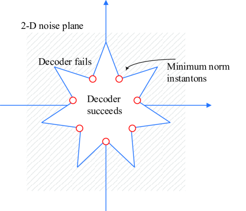
Figure 9: A cartoon showing the idea of instanton.

4.2 Instanton search algorithm for ADMM-PD

We first introduce a specific algorithm for the ADMM penalized decoder denoted by ISA-PD (instanton search algorithm for the penalized decoder). Then we describe a generic algorithm, denoted by ISA-R (instanton search algorithm, refining), which is used to refine the output from ISA-PD. We note that ISA-PD is already able to produce good instanton search results. However ISA-R can still refine the results obtained by ISA-PD. This is demonstrated in Section 4.3.

4.2.1 Specific algorithm for ADMM-PD

In [35], the authors propose an iterative algorithm to find the minimum weight pseudocodeword in the AWGN channel. For each iteration, the algorithm use an LP decoder to decode a noise vector that is calculated in the previous iteration to guarantee that LP decoding would fail. The output from the LP decoder is a pseudocodeword, which is used to calculate the minimum norm noise vector that can produce this failure. This noise vector is then used in the next iteration to be decoded by the LP decoder. The algorithm terminates when it converges or exceeds some maximum number of allowable iterations. This algorithm is executed repeatedly with random initializations in order to get statistics on instantons.

For ADMM-PD, there is no analytical connection between decoder failures and instantons due to the fact that ADMM-PD is trying to solve a non-convex problem. Whenever ADMM-PD fails, the output is not necessarily a vertex of the fundamental polytope. However since both LP decoding and ADMM-PD are minimizing an objective over the same constraint set, we can develop an iterative algorithm similar to [35]. Note that for ADMM-PD, we need a different approach to determine a noise vector for the next iteration. Assuming that the all-zero codeword is transmitted and the decoder’s output is $\bm{\omega}$ for the current iteration, we solve the following optimization problem:

$$\operatornamewithlimits{minimize} \|\bm{n}\|_{2}^{2}$$ (4.2)

$$\operatorname{subject~{}to} \bm{\gamma}(\bm{n})^{T}\bm{\omega}+\sum_{i}g(\omega_{i})\leq Ng(0)$$

where $\bm{\gamma}(\bm{n})$ is the LLR for noise $\bm{n}$ and $N$ is the block length. This problem is solving for the smallest norm noise vector that confuses $\mathbf{0}$ and $\bm{\omega}$. Using standard Lagrange multiplier technique, we can obtain the solution

$$\bm{n}^{*}=\bm{\omega}\left(\frac{1}{\|\bm{\omega}\|_{2}^{2}}\left[\|\bm{\omega}\|_{1}+\frac{\sigma^{2}}{2}\left(Ng(0)-\sum_{i}g(\omega_{i})\right)\right]\right),$$ (4.3)

where $g(\cdot)$ is the same function in (3.1) and can be replaced with the specific penalty used. Note that $\bm{x}^{*}$ is an approximation to the minimum noise vector causing ADMM-PD. ADMM-PD can still fail on a noise vector with smaller norm. One needs to search for the smallest norm noise vector that has the same direction as $\bm{x}^{*}$. This is captured in Algorithm 2. Note that this algorithm may not converge. And, similar to [35], different initializations produce different instantons. One should expect to run the algorithm multiple times to obtain statistics of instantons for ADMM-PD.

Algorithm 2 Instanton Search Algorithm for ADMM-PD (ISA-PD)

1:  Initialize a noise vector $\bm{n}^{0}$ sufficiently large that ADMM-PD fails and outputs a vector $\bm{\omega}^{0}$.

2:  Choose the maximum number of iterations allowed $T$. Choose a tolerance $\epsilon>0$.

3:  for all  $k=1,\dots,T$ do

4:     Let $\bm{w}$ be the solution of problem (4.2) given $\bm{\omega}^{k-1}$.

5:     Search for the smallest scaling factor $a>0$ such that decoder fails with noise $a\bm{w}$.

6:     Assign $\bm{n}^{k}\leftarrow a\bm{w}$.

7:     Let $\bm{\omega}^{k}$ be the output of decoder when decoding the noise vector $\bm{n}^{k}$.

8:     Store $\bm{n}^{k}$ if it is the minimum norm noise vector from all previous trials.

9:     if $\|\bm{n}^{k}-\bm{n}^{k-1}\|_{2}\leq\epsilon$ then

10:        Stop loop.

11:     end if

12:  end for

4.2.2 Using a generic instanton search algorithm as a refining step

Although the “amoeba” minimization algorithm can be applied to any decoder, the cost of using this algorithm is huge. The algorithm not only converges slowly, but also requires memory that scales quadratically with respect to block length. Thus it is infeasible to apply this algorithm to large block length codes.

In this paper, we base our instanton search algorithm, ISA-R, on Nesterov’s random gradient free algorithm (cf. [37]). We denote by $f(\cdot)$ the objective function to minimize. In short, the algorithm in [37] starts at a random initial point $\bm{x}_{0}$. Fix a parameter $\eta>0$ and pick a sequence of positive steps $\{h_{k}\}_{k\geq 0}$. For each iteration $k>0$, a vector $\bm{u}$ is generate following Gaussian distribution with correlation operator $\bm{B}^{-1}$. After that, a random gradient-free oracle is computed:

$$\phi_{\eta}(\bm{x}_{k})=\frac{f(\bm{x}_{k}+\eta\bm{u})-f(\bm{x}_{k})}{\eta}\cdot\bm{B}\bm{u}.$$

Then the next step is determined by

$$\bm{x}_{k+1}=\bm{x}_{k}-h_{k}\bm{B}^{-1}\phi_{\eta}(\bm{x}_{k})$$

This algorithm only requires the two most recent vectors thus consumes much less memory compared to the “amoeba” minimization.

Instead of directly applying this method to the objective function in (4.1), we make three important tweaks: First, we make the objective function have a non-zero gradient when the decoder succeeds:

$$\begin{split}\operatornamewithlimits{minimize}_{\bm{n}}\;(1-\mathbb{I}_{\{\text{decoding succeeds with noise $\bm{n}$}\}})\|\bm{n}\|_{2}^{2}\\ +C\mathbb{I}_{\{\text{decoding succeeds with noise $\bm{n}$}\}}\left(1-\|\bm{n}\|_{2}^{2}\right).\end{split}$$ (4.4)

In other words, for each iteration, we run ADMM-PD using the current noise vector and evaluate (4.4).

Second, we leverage the knowledge learned from ISA-PD. Similar to the case of “amoeba” minimization [15], initialization of ISA-R is crucial in order to obtain small norm instantons. In this paper, we use outputs from Algorithm 2 as the initialization. As we will show in Section 4.3, the instanton search results from ISA-PD tend to have only a few non-zero entries and the rest of the entries are zero. We use this knowledge in our algorithm and only select the random Gaussian search direction in Nesterov’s method to have support on the coordinates for which the entries are non-zero entries.

Third, the indicator function in (4.4) may create a huge step size in ISA-R depending on the constant $C$. Thus we restrict the search step size for each iteration by linearly shrinking the vector $h_{k}\bm{B}^{-1}\phi_{\eta}(\bm{x}_{k})$ if its $\ell_{2}$-norm exceeds some threshold.

4.3 Numerical results of the instanton analysis

We now apply the proposed algorithm to the $[155,64]$ Tanner code [16] and a $[1057,813]$ LDPC code from [17]. For both codes, we obtain instanton information for different penalty coefficients $\alpha_{1}$ and $\alpha_{2}$. We fix parameters (cf. Section 3.4) as follows: $\mu=3$, $T_{\max}=100$, $\epsilon=10^{-5}$, $\rho=1.9$. For each data point, we randomly generate $K=1000$ initial noise vectors with power large enough to cause decoding failures and apply ISA-PD followed by ISA-R. For ISA-R, we use $C=20000$ (cf. (4.1)). For ISA-R, we let $\bm{u}_{k}$ be an Gaussian vector with the identity covariance matrix ($\bm{B}=\bm{I}$), $\eta=10^{-10}$ and $h_{k}=\frac{1}{40000}$. Moreover, we restrict each search step size to have $\ell_{2}$ norm less than or equal to 1.

In Fig. 10, we plot the minimum instanton norm as a function of penalty coefficient $\alpha_{2}$. For each $\alpha_{2}$, we sort the $K$ instantons we find, denoted by $\bm{n}_{i}$, $i=1,...,K$, such that $\|\bm{n}_{1}\|_{2}^{2}\leq\|\bm{n}_{2}\|_{2}^{2}\leq\cdots\leq\|\bm{n}_{K}\|_{2}^{2}$. We then plot the norm $\|\bm{n}_{\phi}\|_{2}^{2}$ where $\phi=K/100=10$ and label it “$1\%$ minimum instanton” in Fig. 10. In order to compare with BP and LP decoding, we plot the effective distance for both decoders. Note that the LP pseudo-distance is actually the norm of the most probable noise that leads to decoding failure (see also [38, Sec. 6]). Results for BP decoding are obtained from [39].

We make the following observations: First, there is a clear trend that as the penalty increases, the minimum instanton norm decreases. This implies that the high-SNR performance of ADMM-PD decreases as the penalty coefficient increases. Second, we observe that the fluctuation of the minimum norm curves increases as $\alpha_{2}$ increases. These fluctuations are partially compensated by ISA-R. We observe that ISA-R makes some refinements at points at $\alpha=0.5,0.8$. It makes a significant refinement at $\alpha=1.8$. This is important because it suggests that the results obtained by ISA-PD for large $\alpha_{2}$ are not accurate especially for $\alpha_{2}\geq 1.6$. Therefore, a curve-fitted worst case instanton norm (shown in in Fig. 11) should predict WER more accurately for large $\alpha_{2}$’s compared to raw data. Thus we suggest using the curve-fitted results. E.g. for $\alpha=2$, results suggest that the minimum instanton norm is $13.8$. We show in Fig. 11 that this result predicts the WER slope well.

In Fig. 11, we plot the WER asymptotics predicted by the minimum norm instanton as well as simulation results. We use $\alpha_{2}=2$ in our simulation because this value is optimal in terms of WER for $\mathrm{SNR}=1.3$ and $1.65$ for this code. All data points are based on more than 100 decoding errors. We make three observations: First, the asymptotics predicted by the minimum instanton norms and the simulated WER curves are almost parallel for each decoder at high SNRs. Second, there are two crossover points in Fig. 11. The first one occurs near $\mathrm{SNR}=1.75$ where LP decoding outperforms BP decoding. The second one occurs near $\mathrm{SNR}=2.3$ where LP decoding outperforms ADMM-PD with an $\ell_{2}$ penalty. This matches our expectation from the instanton results in Fig. 10. Third, the asymptotic curves approximate the slope of the WER. If we were to approximate the actual WER, we would need to compute the multiplicity and the curvature factor of the instantons (cf. [15]). We discuss the multiplicity in Section 4.4.

In Fig. 12, we plot the instanton profile for the $[1057,813]$ code for ADMM-PD with both $\ell_{1}$ and $\ell_{2}$ penalties. We first use the algorithm in [35] to obtain statistics for LP decoding. Based on all instantons we observed, the minimum norm instanton for LP decoding is an actual codeword. This implies that LP decoding is as good as ML decoding at high SNRs for this code, which matches the simulation results obtained in [5]. We make three comments on Fig. 12. First, the algorithm in [35] is not guaranteed to find the minimum weight pseudocodeword. If the weight were actually $7$ for LP decoding then our results would suggest that we can push the penalty coefficient up to $1$ without losing much performance at high SNRs. Second, we observe significant fluctuations in terms of instanton norms. However the one percent instanton norm curves for both penalties decrease monotonically as the penalty coefficients $\alpha_{1}$ and $\alpha_{2}$ increase. The fluctuation is thus due to limited simulation time. Third, ADMM-PD with an $\ell_{1}$ penalty does worse than ADMM-PD with an $\ell_{2}$ penalty for a given parameter $\alpha_{i}$. However, the results obtained in [30] suggest that the optimal $\alpha_{1}$ is less than the optimal $\alpha_{2}$. This implies that both penalties are comparable in terms of instanton norms when each decoder uses its optimal parameter setting.

These results are important in practice. First, although ADMM-PD is observed to outperform LP decoding in [30], it is not as good as LP decoding asymptotically in SNR for nonzero penalty coefficients. Second, in practice, we need to adjust the penalty coefficient as a function of the SNR the code operates at. In particular, we can expect that small penalty coefficients produce better error rate performances at high SNRs, as is shown in Fig. 11.

\psfrag{&A}{\scalebox{0.6}{ penalty coefficient $\alpha_{2}$}}\psfrag{&B}{\scalebox{0.6}{ Instanton norm}}\psfrag{&LP}{\scalebox{0.6}{LP instanton (pseudo-distance)~{}\cite[cite]{[\@@bibref{}{chertkov2008efficient}{}{}]}}}\psfrag{&OnePercentCurveL2padpadpadpadpadpad}{\scalebox{0.6}{$1\%$ minimum instanton}}\psfrag{&MinimumCurveL2}{\scalebox{0.6}{Minimum instanton norm from {ISA-PD}}}\psfrag{&MinimumRefineL2}{\scalebox{0.6}{Refined results from {ISA-R}}}\psfrag{&BP}{\scalebox{0.6}{BP decoding, 100 iterations~{}\cite[cite]{[\@@bibref{}{stepanov2011instantons}{}{}]}}}\psfrag{&curve-fitted}{\scalebox{0.6}{Curve-fitted instanton norm}}\includegraphics[width=252.94499pt]{minimum_instanton_norm.eps}

Figure 10: Instanton norm as a function of penalty coefficient for the $[155,64]$ code when decoded by ADMM-PD with $\ell_{2}$ penalty.

\psfrag{&ADMMLP}{\scalebox{0.6}{ADMM LP decoding}}\psfrag{&BP}{\scalebox{0.6}{Sum-product BP decoding, 100 iterations}}\psfrag{&ADMML2}{\scalebox{0.6}{{ADMM-PD} with $\ell_{2}$ penalty, 100 iterations}}\psfrag{&InstantonPredictionForBP}{\scalebox{0.6}{Asymptote, BP}}\psfrag{&InstantonPredictionForL2-padpadpadpadpadpa}{\scalebox{0.6}{Asymptote, {ADMM-PD} with $\alpha_{2}=2$}}\psfrag{&InstantonPredictionForLP}{\scalebox{0.6}{Asymptote, LP}}\psfrag{&SNR}{\scalebox{0.6}{SNR}}\psfrag{&WER}{\scalebox{0.6}{WER}}\includegraphics[width=252.94499pt]{InstantonSimulation.eps}

Figure 11: Comparisons of simulation results and asymptotic slopes predicted by instantons/pseudocodewords for the $[155,64]$ code. WER is plotted as a function of SNR (not in (dB)). Each asymptote is $\sim\exp(-\|\bm{n}^{\operatorname{inst}}\|_{2}^{2}s^{2}/2)$, where $s^{2}$ is SNR. The value of $\|\bm{n}^{\operatorname{inst}}\|_{2}^{2}$ for BP, ADMM-PD and LP are $11.48$, $13.8$ and $16.35$, respectively.

\psfrag{&A}{\scalebox{0.6}{ penalty coefficient $\alpha_{i}$, $i=1,2$}}\psfrag{&B}{\scalebox{0.6}{ Instanton norm}}\psfrag{&LP}{\scalebox{0.6}{LP pseudo-distance}}\psfrag{&OnePercentCurveL1}{\scalebox{0.6}{$1\%$ minimum instanton, $\ell_{1}$ penalty}}\psfrag{&MinimumCurveL1}{\scalebox{0.6}{Minimum instanton norm, $\ell_{1}$ penalty}}\psfrag{&OnePercentCurveL2padpadpadpadpad}{\scalebox{0.6}{$1\%$ minimum instanton, $\ell_{2}$ penalty}}\psfrag{&MinimumCurveL2}{\scalebox{0.6}{Minimum instanton norm, $\ell_{2}$ penalty}}\includegraphics[width=252.94499pt]{minimum_instanton_norm_1057.eps}

Figure 12: Instanton norm as a function of penalty coefficient for the $[1057,813]$ code when decoded by ADMM-PD.

4.4 Weaknesses of ADMM-PD

It is noticeable from Fig. 12 that the minimum instanton norm (not the $1\%$) stays almost constant for some range of $\alpha$. This suggests that there might be some common structures underlying these instantons, which motivates us to study the patterns of these noise vectors.

We observe that for all minimum norm instantons, there are only a few nonzero entries. Moreover, every instanton we studied has support on trapping set structures widely studied for BP decoders. For the $[155,64]$ code, we observe instantons with non-zeros entries on $(5,3)$ (plotted in Fig. 13) and $(6,4)$ trapping sets. For the $[1057,814]$ code, we observe instantons with non-zeros entries on $(5,1)$ and $(7,1)$ trapping sets. And the $(7,1)$ trapping set contributes to most of the norm $7$ instantons in Fig. 12.

We note two aspects where these results are useful. First, the results imply that we can leverage trapping set knowledge in the literature to compute the multiplicity of a particular instanton. Second, one can expect that code designs that alleviate trapping set effect should also benefit ADMM-PD.

Figure 13: The support of an instanton for the $[155,64]$ code showing a $(5,3)$ trapping set, each node indexed by the variable or check number.

4.5 Remarks

We now briefly discuss our intuition gained from these results. We note that the penalized decoder aims to penalize fractional solutions by adding penalties to the objective on a symbol-by-symbol basis. As a result, the decoder more easily gets stuck at some local configurations such as trapping sets. Meanwhile, increasing the penalty coefficient can decrease the significance of channel evidence during the decoding process. Therefore a small noise can create a bias at the first iteration of decoding that is hard to reverse. So the instanton norm tends to be small for large penalty coefficients.

Next, we note that in ISA-PD, the search direction per iteration is the same as the algorithm proposed in [35]. However for ISA-PD, we need to identify the correct step size along this direction. Nevertheless, we observe from our simulation that (4.3) is a good approximation.

In addition, we note that we would need the curvature information in order to approximate the exact WER for the AWGN channel (cf. [15]). This question has not been studied in the literature and is beyond the scope of this paper. Thus we leave it as a future research direction.

Finally, it is desirable to obtain instanton information for the BSC. However this is not trivial and is beyond the scope of this paper. The reason is that searching for instantons in the BSC can be formulated as a non-convex integer program with feasible set $\{0,1\}^{N}$ and hence is in general intractable unless some knowledge on error patterns are pre-assumed. With our findings that the failures of ADMM-PD is related to trapping set, a natural next step is to study the dynamics of ADMM-PD in trapping sets with the assumption that the underlying channel is the BSC. We leave instanton searching for ADMM-PD in the BSC an open problem.

5 Reweighted LP decoding

In previous sections, we show that ADMM-PD is able to improve the low SNR performance of LP decoding. In addition, ADMM-PD also has good high SNR behaviors. However, unlike LP decoding, it is hard to prove error correction guarantees for ADMM-PD. In this section, we introduce a reweighted LP decoding algorithm derived from ADMM-PD with an $\ell_{1}$ penalty and prove results on error correction guarantees. We use L1PD ($\ell_{1}$ penalized decoding) to denote ADMM-PD with an $\ell_{1}$ penalty and RLPD (reweighted LP decoding) to denote our reweighted LP algorithm. Note that this reweighted LP is different from that in [26] (cf. (2.2)). As a reminder, a comparison is listed in Table 1.

	RLPD	RLPD-KDHVB
# rounds of reweighting	$\geq 2$	2
recovery guarantees	Yes	Yes
BSC	Yes	Yes
AWGN & general MBISO	Yes	No

Table 1: Comparisons between RLPD and RLPD-KDHVB.

5.1 A reweighted LP approximation for L1PD

The general reweighted LP scheme is well known in the compressed sensing community [40]. We are interested in reweighted LPs because it approximates a nonlinear program using a sequence of linear programs thereby bringing a non-convex problem to a sequence of convex problems. We show that the two-round reweighted LP for problem (3.2) has theoretical guarantees. That is, this reweighted LP decoding yields improved recovery threshold than LP decoding for bit flipping channels (cf. [2]).

We briefly summarize the reweighted LP idea in [40]. Consider optimization problem of the following form:

$$\operatornamewithlimits{minimize}_{\bm{v}}\quad\phi(\bm{v})\qquad\operatorname{subject~{}to}\quad\bm{v}\in\mathbb{C},$$

where $\mathbb{C}$ is a convex set. The reweighted LP scheme start from a feasible solution $\bm{v}^{(0)}$ and iteratively solves

$$\bm{v}^{(k+1)}= \operatornamewithlimits{argmin}_{\bm{v}}\quad\phi(\bm{v}^{(k)})+\nabla\phi(\bm{v}^{(k)})\left(\bm{v}-\bm{v}^{(k)}\right)$$ (5.1)

$$\operatorname{subject~{}to}\quad\bm{v}\in\mathbb{C},$$

where $k$ denotes the iterate.

Applying (5.1) to L1PD (cf. (3.2)), we get the following reweighted LP algorithm RLPD. Note that we drop the subscript $\alpha_{1}$ in (3.2) and use only $\alpha$ for simplicity.
$\displaystyle\textbf{RLPD}\qquad\operatornamewithlimits{minimize}$ $\displaystyle\quad\bm{\gamma}^{(k)}(\alpha)^{T}\bm{x}$ (5.2) $\displaystyle\operatorname{subject~{}to}$ $\displaystyle\quad\bm{P}_{j}\bm{x}\in\mathbb{PP}_{d_{j}},\forall j\in\mathcal{J}.$ where $\bm{x}^{(0)}$ is some initialization and $$\bm{\gamma}^{(k)}(\alpha)_{i}=\bm{\gamma}_{i}-\alpha\operatorname{sgn}(x^{(k-1)}_{i}-0.5),\forall i$$

We consider a simple case for our decoding problem: we consider just the two-round version of RLPD. That is, we first solve LP decoding and initialize $\bm{x}^{(0)}$ to be the pseudocodeword $\bm{x}^{(p)}$, then we solve for $\bm{x}^{(1)}$. This scheme is summarized in Algorithm 3. From a theoretical point of view, we show that this two-round RLPD has a better recovery threshold compared to LP decoding. From a practical point of view, the decoding algorithm should be fast in order to perform real time decoding. The cost in terms of efficiency for using multiple-round reweighting could be unacceptable.

Algorithm 3 Two-round RLPD

1:  Solve LP decoding.

2:  if The solution $\bm{x}^{*}$ is an integral solution then

3:     Stop. return $\bm{x}^{*}$.

4:  else

5:     Save pseudocodeword $\bm{x}^{(p)}=\bm{x}^{*}$ and proceed.

6:  end if

7:  for all  $i\in\mathcal{I}$ do

8:     Update $\gamma^{\prime}_{i}\leftarrow\gamma_{i}-\alpha\operatorname{sgn}(x^{(p)}_{i}-0.5)$

9:  end for

10:  Solve

$$\operatornamewithlimits{minimize}\quad\bm{\gamma}^{\prime T}\bm{x}\qquad\operatorname{subject~{}to}\quad\bm{P}_{j}\bm{x}\in\mathbb{PP}_{d_{j}}.$$

Theorem 9

Decoding failures for Algorithm 3 are independent of the codeword that was transmitted.

Proof See Appendix 8.  

5.2 Theoretical guarantees of two-round RLPD

The second LP problem in Algorithm 3 is

$$\begin{split}\operatornamewithlimits{minimize}&\quad\bm{\gamma}^{\prime T}\bm{x}\\ \operatorname{subject~{}to}&\quad\bm{P}_{j}\bm{x}\in\mathbb{PP}_{d_{j}},\end{split}$$ (5.3)

where $\gamma^{\prime}_{i}=\gamma_{i}-\alpha\operatorname{sgn}(x^{(p)}_{i}-0.5)$ and $\alpha>0$ is a constant. Using lemmas introduced in [26], we show that this scheme corrects more errors than LP decoding.

Lemma 10

(Lemma 26 in [38]) The fundamental cone $\mathcal{K}:=\mathcal{K}(\bm{H})$ of parity check matrix $\bm{H}$ is the set of all vectors $\bm{w}\in\mathbb{R}^{n}$ that satisfy

$$w_{i}\geq 0, \forall i\in\mathcal{I},$$

$$w_{i}\leq\sum_{i^{\prime}\in\mathcal{N}_{c}(j)\setminus i}w_{i^{\prime}}, \forall j\in\mathcal{J},\forall i\in\mathcal{I}.$$

Definition 11

(Fundamental Cone Property [26]) Let $\mathcal{F}\subset\{1,2,\dots,n\}$ and $\theta\geq 1$ be fixed. A code $\mathcal{C}$ with parity check matrix $\bm{H}$ is said to have the fundamental cone property $FCP(\mathcal{F},\theta)$, if for every nonzero vector $w\in\mathcal{K}$ the following holds:

$$\theta\|w_{\mathcal{F}}\|_{1}<\|w_{\mathcal{F}^{c}}\|.$$

If for every index set $\mathcal{F}$ of size $k$, $\mathcal{C}$ has the $FCP(\mathcal{F},\theta)$, then we say that $\mathcal{C}$ has $FCP(k,\theta)$.

The key insight of $FCP$ is that when $\theta>1$, even if LP decoding fails, the pseudocodewords still have the nice property described by Lemma 12 below. This turns out to be crucial for reweighted LPs.

Lemma 12

(Lemma 4.1 in [26]) Let $\mathcal{C}$ be a code that has the $FCP(\mathcal{F},\theta)$ for some index set $\mathcal{F}$ and some $\theta\geq 1$. Suppose that a codeword $\bm{x}$ from $\mathcal{C}$ is transmitted through a bit flipping channel, and the received codeword is $\bm{y}$. If the pseudocodeword $\bm{x}^{(p)}$ is the output of the LP decoder for the received codeword $\bm{y}$, then the following holds:

$$\|\bm{x}^{(p)}-\bm{x}\|_{1}<2\frac{\theta+1}{\theta-1}\|(\bm{y}-\bm{x})_{\mathcal{F}^{c}}\|_{1}.$$

Using Lemma. 12, we show our main theorem for two-round RLPD.

Theorem 13

Consider bit flipping channels. If a code $\mathcal{C}$ satisfies $FCP(p_{sd}n,\theta)$ for $\theta>1$ and $p_{sd}>0$ then for all $0<\epsilon<\frac{\theta-1}{4(\theta+1)}$, every error set of size $(1+\epsilon)p_{sd}n$ can be corrected by Algorithm 3.

Proof Assume that the all-zeros codeword is transmitted. Suppose the received vector $\bm{y}$ has $(1+\epsilon)p_{sd}n$ errors. Let $\mathcal{F}\subset\{1,2,\dots,n\}$ be the set of these flipped bits. By Lemma 12,

$$\|\bm{x}^{(p)}\|_{1}<2\frac{\theta+1}{\theta-1}\epsilon p_{sd}n.$$

Let $\mathcal{S}:=\{i|x^{(p)}_{i}<0.5\}$, then

$$\left|\mathcal{S}^{c}\right|<4\frac{\theta+1}{\theta-1}\epsilon p_{sd}n.$$ (5.4)

Let $\epsilon<\frac{\theta-1}{4(\theta+1)}$, then $\left|\mathcal{S}^{c}\right|<p_{sd}n$. Then $\mathcal{C}$ has $FCP(\mathcal{S}^{c},\theta)$. Now rewrite $\bm{\gamma}^{\prime}$ as

$$\gamma_{i}^{\prime}=\left\{\begin{array}[]{rcl}1+\alpha,&&i\in\mathcal{S}\cap\mathcal{F}^{c}\\ 1-\alpha,&&i\in\mathcal{S}^{c}\cap\mathcal{F}^{c}\\ -1-\alpha,&&i\in\mathcal{S}^{c}\cap\mathcal{F}\\ -1+\alpha,&&i\in\mathcal{S}\cap\mathcal{F}\end{array}\right..$$ (5.5)

Let $\alpha>1$, then $\alpha-1<0$. Therefore $\forall\bm{w}\in\mathcal{K}$,

$$\sum_{i}\gamma_{i}^{\prime}w_{i} =\sum_{i\in\mathcal{S}\cap\mathcal{F}^{c}}(1+\alpha)w_{i}+\sum_{i\in\mathcal{S}^{c}\cap\mathcal{F}^{c}}(1-\alpha)w_{i}$$

$$\quad+\sum_{i\in\mathcal{S}^{c}\cap\mathcal{F}}(-1-\alpha)w_{i}+\sum_{i\in\mathcal{S}\cap\mathcal{F}}(-1+\alpha)w_{i}$$

$$>\sum_{i\in\mathcal{S}\cap\mathcal{F}^{c}}(-1+\alpha)w_{i}+\sum_{i\in\mathcal{S}\cap\mathcal{F}}(-1+\alpha)w_{i}$$

$$\quad+\sum_{i\in\mathcal{S}^{c}\cap\mathcal{F}}(-1-\alpha)w_{i}+\sum_{i\in\mathcal{S}^{c}\cap\mathcal{F}^{c}}(-1-\alpha)w_{i}$$

$$=\sum_{i\in\mathcal{S}}(-1+\alpha)w_{i}+\sum_{i\in\mathcal{S}^{c}}(-1-\alpha)w_{i}$$

$$=(\alpha-1)\left[\sum_{i\in\mathcal{S}}w_{i}-\frac{\alpha+1}{\alpha-1}\sum_{i\in\mathcal{S}^{c}}w_{i}\right]$$

$$=(\alpha-1)\left[\|w_{\mathcal{S}}\|_{1}-\frac{\alpha+1}{\alpha-1}\|w_{\mathcal{S}^{c}}\|_{1}\right].$$

Since $\mathcal{C}$ has $FCP(\mathcal{S}^{c},\theta)$, pick $\alpha>\frac{\theta+1}{\theta-1}$, then $1<\frac{\alpha+1}{\alpha-1}<\theta$ and

$$\|w_{\mathcal{S}}\|_{1}-\frac{\alpha+1}{\alpha-1}\|w_{\mathcal{S}^{c}}\|_{1}>\|w_{\mathcal{S}}\|_{1}-\theta\|w_{\mathcal{S}^{c}}\|_{1}>0.$$

Therefore $\sum_{i}\gamma_{i}^{\prime}w_{i}>0$ for all $\bm{w}\in\mathcal{K}$. This implies that the all-zeros solution is the minimizer. Then LP problem (5.3) recovers the all-zeros codeword.  

Corollary 14

Let $\mathcal{G}$ be the factor graph of a code $\mathcal{C}$ of length $n$ and the rate $R=\frac{m}{n}$, and let $\delta>2/3+1/c$. If $\mathcal{G}$ is a bipartite $(\alpha n,\delta c)$ expander graph, then Algorithm 3 succeeds, as long as at most $t(1+\epsilon)n$ bits are flipped by the channel, where $t=\frac{3\delta-2}{2\delta-1}\alpha$ and $\epsilon=\frac{1}{16\delta c-8c-4}$.

Proof By Theorem 5.1 in [26], $FCP(tn,\theta)$ holds, where $\theta=\frac{2\delta-1}{2\delta-1-1/c}$. Then by Theorem 13, we can correct $(1+\epsilon)tn$ errors.  

5.3 A special case of two-round RLPD

We now examine the reweighted LP obtained by letting $\alpha\rightarrow\infty$. The algorithm is summarized in Algorithm 4. We can consider the linear program (5.6) as the LP decoding under a new bit flipping channel, where the output of the channel is determined solely by penalizing pseudocodewords.

Algorithm 4 Two-round RLPD, $\alpha=+\infty$

1:  Solve LP decoding.

2:  if The solution $\bm{x}^{(0)}$ is an integral solution then

3:     Stop. return $\bm{x}^{(0)}$.

4:  else

5:     Save the pseudocodeword $\bm{x}^{(p)}=\bm{x}^{(0)}$ and proceed.

6:  end if

7:  for all  $i\in\mathcal{I}$ do

8:     Update $\gamma^{\prime}_{i}=-\operatorname{sgn}(x^{(p)}_{i}-0.5)$.

9:  end for

10:  Solve

$$\begin{split}\operatornamewithlimits{minimize}&\quad\bm{\gamma}^{\prime T}\bm{x}\\ \operatorname{subject~{}to}&\quad\bm{P}_{j}\bm{x}\in\mathbb{PP}_{d_{j}}.\end{split}$$ (5.6)

Corollary 15

Theorem 13 also holds for Algorithm 4.

Proof The only difference between this proof and proof for Theorem 13 is the values for $\bm{\gamma}^{\prime}$ in (5.5). The new values are

$$\gamma_{i}^{\prime}=\left\{\begin{array}[]{rcl}\alpha,&&i\in T\\ -\alpha,&&i\in T^{c}\end{array}\right..$$

Then we can normalize the objective and let $\alpha=\pm 1$. Using $FCP$, we immediately deduce that this LP recovers the all-zero codeword.  

Note that Theorem 13 is conservative since the proof considers the worst case scenario. Probabilistic analyses introduced in [3] and [4] cannot be applied directly to this case because the second LP takes the pseudocodeword that results from the first LP as part of its input. The probabilistic properties for pseudocodewords should not be considered to be the same as the received vectors from a memoryless channel. Thus, probabilistic analyses for reweighted LP decoding remains open.

5.4 Numerical results of RLPD

In this section, we show numerical results for error performance of RLPD. In Fig. 14, we again simulate the $[2640,1320]$ Margulis code using two-round RLPD and compare its performance to other decoders. We make the following observations: First, two-round RLPD outperforms LP decoding significantly (by around $0.3\mathrm{dB}$) even though the provable improvement presented in the previous section is small. This shows that RLPD is a good practical decoding algorithm for decoding LDPC codes. Second, there is still a $0.3\mathrm{dB}$ SNR gap between L1PD and two-round RLPD. Since two-round RLPD solves two LPs, each with complexity similar to L1PD, it is still desirable to apply L1PD in practice. Interested readers are referred to [41] for simulation results for the BSC.

\psfrag{&ADMMLP}{\scalebox{0.6}{ADMM LP decoding}}\psfrag{&ADMM-ReweightedLP}{\scalebox{0.6}{Two-round {RLPD}}}\psfrag{&BPNonSat}{\scalebox{0.6}{Non-saturating BP decoding}}\psfrag{&&ADMM-L1PenaliedDecoder}{\scalebox{0.6}{{ADMM-PD}, $\ell_{1}$ penalty }}\psfrag{&G}{\scalebox{0.6}{$E_{b}/N_{0}(\mathrm{dB})$}}\psfrag{&H}{\scalebox{0.6}{WER}}\psfrag{1}{\scriptsize{$1$}}\psfrag{1.5}{\scriptsize{$1.5$}}\psfrag{2}{\scriptsize{$2$}}\psfrag{2.5}{\scriptsize{$2.5$}}\psfrag{3}{\scriptsize{$3$}}\psfrag{10}{\scriptsize{$10$}}\psfrag{-2}{\tiny{$-2$}}\psfrag{-4}{\tiny{$-4$}}\psfrag{-6}{\tiny{$-6$}}\psfrag{-8}{\tiny{$-8$}}\psfrag{e0}{\tiny{$0$}}\includegraphics[width=252.94499pt]{MargulisCodeAWGN_RLP.eps}

Figure 14: Word-error-rate (WER) of the $[2640,1320]$ “Margulis” code plotted as a function of $E_{b}/N_{0}$ for the AWGN channel.

We also study the impact of allowing multiple rounds for RLPD. In Fig. 15, we plot the WER performance as a function of the number of rounds allowed for RLPD. From this experiment, we conclude that by allowing multiple rounds for RLPD, we can achieve better error performance. However the gain from every additional round of reweighting decreases as the number of rounds increases. But even with 10 rounds, the RLPD cannot surpass BP decoding or ADMM-PD, making it less favorable in scenarios where provable guarantees are not necessary.

\psfrag{&LPDecoder}{\scalebox{0.6}{LP decoding}}\psfrag{&MultipleRoundsRLP}{\scalebox{0.6}{{RLPD}, $\alpha=0.6$}}\psfrag{&NonsatBP}{\scalebox{0.6}{Non-saturating BP}}\psfrag{&L1PD}{\scalebox{0.6}{{L1PD}, $\alpha=0.6$}}\psfrag{&G}{\scalebox{0.6}{ \# of rounds for {RLPD}}}\psfrag{&H}{\scalebox{0.6}{ word-error-rate (WER)}}\includegraphics[width=252.94499pt]{MargulisCodeAWGN_RLP_Rounds.eps}

Figure 15: Effects of multiple-round reweighting. The word-error-rate (WER) of the $[2640,1320]$ “Margulis” code for the AWGN channel is plotted as a function of # of rounds of reweightings. $E_{b}/N_{0}=2.2\mathrm{dB}$.

6 Conclusions

In this paper, we introduce a class of high performing decoders for LDPC codes. The key idea is the addition of a penalty term to the linear objective of LP decoding with the intent of suppressing pseudocodewords.

We show that by constructing an objective that includes an $\ell_{1}$ or an $\ell_{2}$ penalty we are able to decode LDPC codes in a way that combines the best characteristics of BP and LP decoders. We summarize the advantages of the ADMM penalized decoders. First, in our simulations, the decoders associated with both $\ell_{1}$ and $\ell_{2}$ penalties close the SNR gap between LP and BP decoding. They either achieve (for the MacKay code) or outperform (for the Margulis code) BP at low SNRs. Second, the ADMM penalized decoder has similar WER slope as LP decoding at high SNRs, steeper than BP decoding which suffers from an error floor. Third, the ADMM penalized decoder attains good error performance with no sacrifices in decoding speed. On the contrary, it outperforms both BP and LP decoding in terms of decoding speed in our software serial implementation. All these aspects make the ADMM penalized decoder a strong competitor in practice to both BP and LP decoding.

The objective function of the decoding problem is non-convex. To analyze this non-convex decoder, we use the concept of instantons. We extend the instanton search algorithms in the literature to the ADMM penalized decoder. Using the instanton search algorithm, we show that we can accurately predict the high SNR behavior of the ADMM penalized decoder. In order to regain provable error correction guarantees similar to the LP decoder, we linearize the penalized objective thereby bringing the problem to the convex realm. When applied to bit flipping channels, we show that this linearized problem has better theoretical guarantees when compared to the LP decoder. In addition, we show through simulation results that it significantly outperforms LP decoding.

We identify several future directions of this decoder. We show in this paper that decoding failures are, again, related to trapping sets. Therefore understanding the dynamics of ADMM on trapping sets can be useful for better predicting the high SNR performance of the decoder. This is left for future work. Moreover, even for non-convex programs, it may be possible to prove convergence under some special conditions. This question is open and is left for future work. Since this decoder achieves the best performance compared to both LP and BP decoding, it is natural to ask whether it can be efficiently implemented in hardware. This makes for a third future direction.

Appendix

7 Proof of theorem 6 and corollary 7

7.1 Proof of theorem 6

We first sketch the proof without proving a key lemma: Lemma 16. Then we prove Lemma 16. Proof We need to prove $P[\mathrm{error}|0^{n}]=P[\mathrm{error}|\bm{c}]$, where $\bm{c}$ is any non-zero codeword. Let

$$\mathcal{B}(\bm{c}):=\{\bm{y}|\text{Decoder fails to recover }\bm{c}\text{ if }\bm{y}\text{ is received}\}$$

Then $P[\mathrm{error}|\bm{c}]=\sum_{y\in\mathcal{B}(c)}P[\bm{y}|\bm{c}]$. We show in Lemma 16 that for any codeword $\bm{c}$, there exists a one-to-one mapping from the received vector $\bm{y}$ to a vector $\bm{y}^{0}$, such that the following two statements hold:

1. $P[\bm{y}|\bm{c}]=P[\bm{y}^{0}|0^{n}]$,

2. $\bm{y}\in\mathcal{B}(\bm{c})$ if and only if $\bm{y}^{0}\in\mathcal{B}(0^{n})$.

Then

$$P[\mathrm{error}|\bm{c}] =\sum_{\bm{y}\in\mathcal{B}(\bm{c})}P[\bm{y}|\bm{c}]$$

$$=\sum_{\bm{y}^{0}\in\mathcal{B}(0^{n})}P[\bm{y}^{0}|\bm{c}]=P[\mathrm{error}|0^{n}]$$

Lemma 16 explicitly describes the mapping that satisfies both two statements above and completes the proof.  

Lemma 16

Let $\bm{c}$, $\bm{y}$ and $\mathcal{B}(\bm{c})$ be defined the same way as above. Let $\mathsf{Z}:\Sigma^{n}\mapsto\Sigma^{n}$ be a mapping and $\bm{y}^{0}:=\mathsf{Z}(\bm{y})$ is defined by

$$y^{0}_{i}=\begin{cases}y_{i}&\text{if $c_{i}=0$,}\\ y_{i}^{\prime}&\text{if $c_{i}=1$.}\end{cases}$$

where $y_{i}^{\prime}$ is the symmetric symbol of $y_{i}$ with respect to the symmetric channel $P_{Y|X}$. Then

1. $P[\bm{y}|\bm{c}]=P[\bm{y}^{0}|0^{n}]$,

2. $\bm{y}\in\mathcal{B}(\bm{c})$ if and only if $\bm{y}^{0}\in\mathcal{B}(0^{n})$.

Proof

• Proof of statement (1):

  $$P[\bm{y}|\bm{c}] =\prod_{i}P[y_{i}|c_{i}]$$

  $$=\prod_{i:c_{i}=0}P[y_{i}|0]\prod_{i:c_{i}=1}P[y_{i}|1]$$

  $$=\prod_{i:c_{i}=0}P[y^{0}_{i}|0]\prod_{i:c_{i}=1}P[y_{i}^{\prime}|0]$$

  $$=\prod_{i}P[y^{0}_{i}|0]=P[\bm{y}^{0}|0^{n}]$$

• Proof of statement (2): We first define relative vector. The definition here is slightly different from the definition in [1].

  Definition 17

  The relative vector of a vector $\bm{a}\in\mathbb{R}^{N}$ with respect to codeword $\bm{c}$ of length $N$ is denoted by $\bm{a}^{r}:=\mathsf{R}_{\bm{c}}(\bm{a})$, which is obtained as

  $$\mathsf{R}_{\bm{c}}(\bm{a})_{i}=\begin{cases}a_{i}&\text{if $c_{i}=0$,}\\ 1-a_{i}&\text{if $c_{i}=1$.}\end{cases}$$

  One special yet useful case is $\mathsf{R}_{\bm{c}}(\bm{c})=0^{n}$.

  With a small abuse of notation, we allow operator $\mathsf{R}$ take replicas of ADMM formulation $\bm{z}_{j}$ as input. Since the entries in $\bm{z}_{j}$ are inherently associated with indices of the codeword $\bm{c}$, $\mathsf{R}_{\bm{c}}(\bm{z}_{j})$ defines the relative vector of $\bm{z}_{j}$ with respect to the corresponding sub-vector (defined by the $j$-th check) of $\bm{c}$.

  Now let $\hat{\bm{c}}:=\mathscr{D}(\bm{y})$ be the output of the decoder if $\bm{y}$ is received and $\hat{\bm{c}}^{0}:=\mathscr{D}(\bm{y}^{0})$. We show in Lemma 19 that $\hat{\bm{c}}^{0}=\mathsf{R}_{\bm{c}}(\hat{\bm{c}})$. Then $\mathscr{D}(\bm{y})=\bm{c}$ if and only if $\mathscr{D}(\bm{y}^{0})=\mathsf{R}_{\bm{c}}(\bm{c})=0^{n}$, which implies the second statement.

 

Lemma 18

In Algorithm 1, let $\bm{x}^{(k)}$, $\bm{z}_{j}^{(k)}$ and $\bm{\lambda}_{j}^{(k)}$ be the vectors after the $k$-th iteration when decoding $\bm{y}$. Let $\bm{x}^{0,(k)}$, $\bm{z}_{j}^{0,(k)}$ and $\bm{\lambda}_{j}^{0,(k)}$ be the vectors after the $k$-th iteration when decoding $\bm{y}^{0}$. If $\bm{x}^{(k)}=\mathsf{R}_{\bm{c}}(\bm{x}^{0,(k)})$, $\bm{z}_{j}^{(k)}=\mathsf{R}_{\bm{c}}(\bm{z}_{j}^{0,(k)})$ and $\bm{\lambda}_{j}^{(k)}=-\bm{\lambda}_{j}^{0,(k)}$ then $\bm{x}^{(k+1)}=\mathsf{R}_{\bm{c}}(\bm{x}^{0,(k+1)})$, $\bm{z}_{j}^{(k+1)}=\mathsf{R}_{\bm{c}}(\bm{z}_{j}^{0,(k+1)})$ and $\bm{\lambda}_{j}^{(k+1)}=-\bm{\lambda}_{j}^{0,(k+1)}$.

Proof We drop the iterate $(k)$ for simplicity and denote $\bm{x}^{\mathrm{new}}$ , $\bm{z}_{j}^{\mathrm{new}}$ and $\bm{\lambda}^{\mathrm{new}}_{j}$ to be the updated vector at $(k+1)$-th iteration. Let $\bm{x}=\mathsf{R}_{\bm{c}}(\bm{x}^{0})$, $\bm{z}_{j}=\mathsf{R}_{\bm{c}}(\bm{z}_{j}^{0})$ and $\bm{\lambda}_{j}=-\bm{\lambda}_{j}^{0}$. Also let $\bm{\gamma}^{0}$ be the log-likelihood ratio for the received vector $\bm{y}^{0}$. At the $\bm{x}$-update, it is sufficient to verify indices $i$ where $c_{i}=1$. From Algorithm 1, $x_{i}^{\mathrm{new}}$ is the root with the maximum distance from $0.5$ of the following equation

$$x=\frac{1}{|\mathcal{N}_{v}(i)|}\left(\sum_{j}\left(\bm{z}_{j}^{(i)}-\frac{\bm{\lambda}_{j}^{(i)}}{\mu}\right)-\frac{1}{\mu}(\gamma_{i}+g^{\prime}(x))\right).$$ (7.1)

By the symmetry property of the penalty function $g$, $1-x_{i}^{\mathrm{new}}$ is the root of equation

$$x=\frac{1}{|\mathcal{N}_{v}(i)|}\left(\sum_{j}\left(1-\bm{z}_{j}^{(i)}+\frac{\bm{\lambda}_{j}^{(i)}}{\mu}\right)+\frac{1}{\mu}(\gamma_{i}-g^{\prime}(x))\right).$$ (7.2)

Since the channel is symmetric, $\bm{\gamma}=-\bm{\gamma}^{0}$. Then (7.2) can be rewritten as

$$x=\frac{1}{|\mathcal{N}_{v}(i)|}\left(\sum_{j}\left(\bm{z}_{j}^{0,(i)}-\frac{\bm{\lambda}_{j}^{0,(i)}}{\mu}\right)-\frac{1}{\mu}(\gamma_{i}^{0}+g^{\prime}(x))\right).$$ (7.3)

Suppose there exists another root $t$ for equation (7.3) such that $|t-0.5|>|(1-x_{i}^{\mathrm{new}})-0.5|$ then $1-t$ is a root for equation (7.1), contradicting with the fact that $x_{i}^{\mathrm{new}}$ is the root of equation (7.1) that has the largest distance from 0.5. Therefore

$$x_{i}^{\mathrm{new}}=1-x_{i}^{\mathrm{new},0}$$

Let $\bm{v}_{j}=\bm{P}_{j}\bm{x}+\bm{\lambda}_{j}/\mu$ and $\bm{v}^{0}_{j}=\bm{P}_{j}\bm{x}^{0}+\bm{\lambda}^{0}_{j}/\mu$, then $\bm{v}^{0,(i)}_{j}=1-(\bm{P}_{j}\bm{x})^{(i)}-\bm{\lambda}^{(i)}_{j}/\mu=1-\bm{v}^{(i)}_{j}$. Now $\bm{z}^{\mathrm{new}}_{j}=\Pi_{\mathbb{PP}_{d}}(\bm{v}_{j})$ and $\bm{z}^{0,\mathrm{new}}_{j}=\Pi_{\mathbb{PP}_{d}}(\bm{v}^{0}_{j})$. This means that we need to show $\bm{z}^{\mathrm{new}}_{j}=\mathsf{R}_{\bm{c}}(\bm{z}^{0,\mathrm{new}}_{j})$. In order to show this, we use Lemma 17 in [1].

Suppose the the opposite is true, that is $\bm{z}^{0,\mathrm{new}}_{j}$ is the projection of $\bm{v}^{0}_{j}$ onto the parity polytope, but $\mathsf{R}_{\bm{c}}(\bm{z}^{0,\mathrm{new}}_{j})$ is not the projection of $\bm{v}_{j}$. By Lemma 17 in [1], $\mathsf{R}_{\bm{c}}(\bm{z}^{0,\mathrm{new}}_{j})$ is inside the parity polytope. Suppose the real projection is $\bm{z}_{j}^{\prime}$, then $\mathsf{R}_{\bm{c}}(\bm{z}_{j}^{\prime})$ is also in the parity polytope and

$$\|\mathsf{R}_{\bm{c}}(\bm{z}_{j}^{\prime})-\bm{v}^{0}_{j}\|_{2} =\|\bm{z}_{j}^{\prime}-\bm{v}_{j}\|_{2}$$

$$<\|\mathsf{R}_{\bm{c}}(\bm{z}^{0,\mathrm{new}}_{j})-\bm{v}_{j}\|_{2}=\|\bm{z}^{0,\mathrm{new}}_{j}-\bm{v}^{0}_{j}\|_{2}$$

Now $\mathsf{R}_{\bm{c}}(\bm{z}_{j}^{\prime})$ is closer to $\bm{v}_{j}^{0}$ than $\bm{z}^{0,\mathrm{new}}_{j}$ is. This contradicts the assumption that $\bm{z}^{0,\mathrm{new}}_{j}$ is the projection.

It remains to verify one more equality:

$$\bm{\lambda}^{\mathrm{new},(i)}_{j} =\bm{\lambda}^{(i)}_{j}+\mu\left((\bm{P}_{j}\bm{x}^{\mathrm{new}})^{(i)}-\bm{z}_{j}^{\mathrm{new},(i)}\right)$$

$$=-\bm{\lambda}^{0,(i)}_{j}+\mu\left(\left(1-(\bm{P}_{j}\bm{x}^{0,\mathrm{new}})^{(i)}\right)\right.$$

$$\quad-\left.\left(1-\bm{z}_{j}^{0,\mathrm{new},(i)}\right)\right)$$

$$=-\left(\bm{\lambda}^{0,(i)}_{j}+\mu\left((\bm{P}_{j}\bm{x}^{0,\mathrm{new}})^{(i)}-\bm{z}_{j}^{0,\mathrm{new},(i)}\right)\right)$$

$$=-\bm{\lambda}^{0,\mathrm{new},(i)}_{j}$$

 

Lemma 19

Let $\hat{\bm{c}}=\mathscr{D}(\bm{y})$ be the output of the decoder if $\bm{y}$ is received and $\hat{\bm{c}}^{0}=\mathscr{D}(\bm{y}^{0})$. Then $\hat{\bm{c}}^{0}=\mathsf{R}_{\bm{c}}(\hat{\bm{c}})$.

Proof We drop the iteration number $k$ for simplicity. Note that for all $j$, $\bm{\lambda}_{j}$ and $\bm{z}_{j}$ are initialized such that $\bm{z}_{j}=\mathsf{R}_{\bm{c}}(\bm{z}_{j}^{0})=0.5$ and $\bm{\lambda}_{j}=-\bm{\lambda}_{j}^{0}=0$. By induction on Lemma 18, Lemma 18 holds for all iterations. It remains to prove that both decoding processes stop at the same iteration. When determining the termination criterion,

$$\left|\left(\bm{P}_{j}\bm{x}\right)_{i}-\left(\bm{z}_{j}\right)_{i}\right| =\left|\left(1-\left(\bm{P}_{j}\bm{x}\right)_{i}\right)-\left(1-\left(\bm{z}_{j}\right)_{i}\right)\right|$$

$$=\left|\left(\bm{P}_{j}\bm{x}\right)^{r}_{i}-\left(\bm{z}_{j}\right)^{r}_{i}\right|=\left|\left(\bm{P}_{j}\bm{x}^{0}\right)_{i}-\left(\bm{z}^{0}_{j}\right)_{i}\right|$$

Therefore

$$\sum_{j}{\|\bm{P}_{j}\bm{x}-\bm{z}_{j}\|^{2}_{2}}=\sum_{j}{\|\bm{P}_{j}\bm{x}^{0}-\bm{z}_{j}^{0}\|^{2}_{2}}$$

and

$$\sum_{j}{\|\bm{z}^{k}_{j}-\bm{z}^{k-1}_{j}\|^{2}_{2}}=\sum_{j}{\|\bm{z}^{k,0}_{j}-\bm{z}^{k-1,0}_{j}\|^{2}_{2}}$$

for every iteration. This implies decoding $\bm{y}$ and $\bm{y}^{0}$ will terminate at the same iterate. The output of the decoder, $\mathscr{D}(\bm{y})$ and $\mathscr{D}(\bm{y}^{0})$, will then be relative vectors according to Lemma 18. Therefore $\hat{\bm{c}}^{0}=\mathsf{R}_{\bm{c}}(\hat{\bm{c}})$.  

7.2 Proof of corollary 7

1. Proof for the first case.

   Lemma 19 still holds if the initialized vectors $\bm{z}_{j}^{(0)}=\mathsf{R}_{\bm{c}}(\bm{z}_{j}^{0,(0)})$ and $\bm{\lambda}_{j}^{(0)}=-\bm{\lambda}_{j}^{0,(0)}=0$. For any initial vector for decoding $\bm{y}^{0}$, there exist a initial vector for decoding $\bm{y}$ that has the same decoding failure probability. Since $\bm{z}_{j}$ is initialized uniformly, the total probability of error is the same.

2. Proof for the second case.

   Lemma 20

   In LP decoding (2.1), let $\hat{\bm{c}}=\mathscr{D}(\bm{y})$ be the output of the decoder if $\bm{y}$ is received and $\hat{\bm{c}}^{0}=\mathscr{D}(\bm{y}^{0})$. Then $\hat{\bm{c}}^{0}=\mathsf{R}_{\bm{c}}(\hat{\bm{c}})$.

   Proof Let $\hat{\bm{c}}_{r}:=\mathsf{R}_{\bm{c}}(\hat{\bm{c}})$. By Lemma 18 in [1],

   $$\sum_{i}\gamma_{i}\hat{c}_{i}-\sum_{i}\gamma_{i}y_{i}=\sum_{i}\gamma_{i}^{0}\hat{c}_{r,i}-\sum_{i}\gamma_{i}^{0}0.$$

   Suppose that the opposite is true, that is $\hat{\bm{c}}^{0}\neq\hat{\bm{c}}_{r}$, then

   $$\sum_{i}\gamma_{i}^{0}\hat{c}^{0}_{i}<\sum_{i}\gamma_{i}^{0}\hat{c}_{r,i}=\sum_{i}\gamma_{i}\hat{c}_{i}-\sum_{i}\gamma_{i}y_{i}.$$

   Let $\hat{\bm{c}}^{0}_{r}:=\mathsf{R}_{\bm{c}}(\hat{\bm{c}}^{0})$. Then $\hat{\bm{c}}^{0}_{r}$ is feasible by Lemma 17 in [1]. Then

   $$\sum_{i}\gamma_{i}^{0}\hat{c}^{0}_{r,i}-\sum_{i}\gamma_{i}y_{i} =\sum_{i}\gamma_{i}^{0}\hat{c}^{0}_{i}-\sum_{i}\gamma_{i}^{0}0$$

   $$<\sum_{i}\gamma_{i}\hat{c}_{i}-\sum_{i}\gamma_{i}y_{i},$$

   which implies that

   $$\sum_{i}\gamma_{i}^{0}\hat{c}^{0}_{r,i} <\sum_{i}\gamma_{i}\hat{c}_{i}$$

   This means that $\hat{\bm{c}}$ is not the minimizer, contradicting the fact that it is the output of the LP decoder.  

   With lemma 20, the initialized vectors satisfies $\bm{z}_{j}^{(0)}=\mathsf{R}_{\bm{c}}(\bm{z}_{j}^{0,(0)})$ and $\bm{\lambda}_{j}^{(0)}=-\bm{\lambda}_{j}^{0,(0)}=0$. Thus by lemma 19, Theorem 6 still holds.

8 Proof of Theorem 9

Proof There are two cases: (i) the decoder outputs an integral solution in the first LP and terminates or (ii) the decoder proceeds to the reweighted LP step. For the first case, the decoding error probability is independent of the transmitted codeword by standard LP decoding results [1]. For the second case, we only need to show that $\bm{\gamma}^{\prime}=-\bm{\gamma}^{\prime,0}$. Then by Lemma 20, we still get relative solutions, and therefore are equivalent. Let $\bm{x}^{(p)}_{r}:=\mathsf{R}_{\bm{c}}(\bm{x}^{(p)})$, then

$$\gamma^{\prime}_{i} =\gamma_{i}+g^{\prime}(x^{(p)}_{i})$$

$$=-\gamma_{i}^{0}-g^{\prime}(x^{(p)}_{r,i})$$

$$=-\gamma_{i}^{\prime,0}$$

where the second equality comes from that $g$ is symmetric at $x=0.5$, so that $g^{\prime}(x)=-g^{\prime}(1-x)$.

References

- [1] J. Feldman, M. Wainwright, and D. Karger, “Using linear programming to decode binary linear codes,” IEEE Trans. Inf. Theory, vol. 51, no. 3, pp. 954–972, Mar. 2005.
- [2] J. Feldman, T. Malkin, R. A. Servedio, C. Stein, and M. J. Wainwright, “LP decoding corrects a constant fraction of errors,” IEEE Trans. Inf. Theory, vol. 53, no. 1, pp. 82–89, Jan. 2007.
- [3] C. Daskalakis, A. Dimakis, R. Karp, and M. Wainwright, “Probabilistic analysis of linear programming decoding,” IEEE Trans. Inf. Theory, vol. 54, no. 8, pp. 3565–3578, Aug. 2008.
- [4] S. Arora, C. Daskalakis, and D. Steurer, “Message-passing algorithms and improved LP decoding,” IEEE Trans. Inf. Theory, vol. 58, no. 12, pp. 7260–7271, Dec. 2012.
- [5] S. Barman, X. Liu, S. Draper, and B. Recht, “Decomposition methods for large scale LP decoding,” IEEE Trans. Inf. Theory, vol. 59, no. 12, pp. 7870–7886, Dec. 2013.
- [6] P. O. Vontobel and R. Koetter, “Towards low complexity linear programming decoding,” in Proc. 4th Int. Symp. Turbo Codes and Related Topics, Munich, Germany, Apr. 2006, pp. 1–9.
- [7] M.-H. Taghavi and P. Siegel, “Adaptive methods for linear programming decoding,” IEEE Trans. Inf. Theory, vol. 54, no. 12, pp. 5396–5410, Dec. 2008.
- [8] D. Burshtein, “Iterative approximate linear programming decoding of LDPC codes with linear complexity,” IEEE Trans. Inf. Theory, vol. 55, no. 11, pp. 4835–4859, Nov. 2009.
- [9] M. Taghavi, A. Shokrollahi, and P. Siegel, “Efficient implementation of linear programming decoding,” IEEE Trans. Inf. Theory, vol. 57, no. 9, pp. 5960–5982, Sept. 2011.
- [10] X. Zhang and P. H. Siegel, “Efficient iterative LP decoding of LDPC codes with alternating direction method of multipliers,” in IEEE Int. Symp. inf. Theory (ISIT), July 2013, pp. 1501–1505.
- [11] G. Zhang, R. Heusdens, and W. Kleijn, “Large scale LP decoding with low complexity,” IEEE Commun. Lett., vol. 17, no. 11, pp. 2152–2155, Oct. 2013.
- [12] N. Derbinsky, J. Bento, V. Elser, and J. S. Yedidia, “An improved three-weight message-passing algorithm,” ArXiv preprint 1305.1961, May 2013.
- [13] P. Vontobel, “Counting in graph covers: A combinatorial characterization of the bethe entropy function,” IEEE Trans. Inf. Theory, vol. 59, no. 9, pp. 6018–6048, Sept. 2013.
- [14] M. Stepanov and M. Chertkov, “Instanton analysis of low-density parity-check codes in the error-floor regime,” in IEEE Int. Symp. inf. Theory, 2006, pp. 552–556.
- [15] S. Chilappagari, M. Chertkov, M. Stepanov, and B. Vasic, “Instanton-based techniques for analysis and reduction of error floors of LDPC codes,” IEEE J. Sel. Areas Commun., vol. 27, no. 6, pp. 855–865, July 2009.
- [16] R. M. Tanner, D. Sridhara, and T. Fuja, “A class of group-structured LDPC codes,” in ICSTA, Ambleside, UK, 2001.
- [17] D. J. C. MacKay, “Encyclopedia of sparse graph codes,” available online at http://www.inference.phy.cam.ac.uk/mackay/codes/data.html.
- [18] D. J. C. MacKay and M. S. Postol, “Weaknesses of Margulis and Ramanujan-Margulis low-density parity-check codes,” Electronic Notes in Theoretical Computer Science, vol. 74, pp. 97–104, 2003.
- [19] Y. Wang, S. Draper, and J. Yedidia, “Hierarchical and high-girth QC LDPC codes,” IEEE Trans. Inf. Theory, vol. 59, no. 7, pp. 4553–4583, Jul. 2013.
- [20] A. Tanatmis, S. Ruzika, H. Hamacher, M. Punekar, F. Kienle, and N. Wehn, “A separation algorithm for improved LP decoding of linear block codes,” IEEE Trans. Inf. Theory, vol. 56, no. 7, pp. 3277–3289, July 2010.
- [21] A. Dimakis, A. Gohari, and M. Wainwright, “Guessing facets: Polytope structure and improved LP decoder,” IEEE Trans. Inf. Theory, vol. 55, no. 8, pp. 3479–3487, Aug. 2009.
- [22] A. Yufit, A. Lifshitz, and Y. Be’ery, “Efficient linear programming decoding of hdpc codes,” IEEE Trans. Commun., vol. 59, no. 3, pp. 758–766, March 2011.
- [23] X. Zhang and P. Siegel, “Adaptive cut generation algorithm for improved linear programming decoding of binary linear codes,” IEEE Trans. Inf. Theory, vol. 58, no. 10, pp. 6581–6594, Oct. 2012.
- [24] S. Draper, J. Yedidia, and Y. Wang, “ML decoding via mixed-integer adaptive linear programming,” in IEEE Int. Symp. inf. Theory (ISIT), June 2007, pp. 1656–1660.
- [25] M. Helmling, S. Ruzika, and A. Tanatmis, “Mathematical programming decoding of binary linear codes: Theory and algorithms,” IEEE Trans. Inf. Theory, vol. 58, no. 7, pp. 4753–4769, July. 2012.
- [26] A. Khajehnejad, A. Dimakis, B. Hassibi, B. Vigoda, and W. Bradley, “Reweighted LP decoding for LDPC codes,” IEEE Trans. Inf. Theory, vol. 58, no. 9, pp. 5972–5984, Sep. 2012.
- [27] S. Boyd, N. Parikh, E. Chu, B. Peleato, and J. Eckstein, “Distributed optimization and statistical learning via the alternating direction method of multipliers,” Machine Learning, vol. 3, no. 1, pp. 1–123, 2010.
- [28] R. Tibshirani, “Regression shrinkage and selection via the Lasso,” J. Roy. Statist. Soc. Ser. B., vol. 58, no. 1, pp. 267–288, 1996.
- [29] T. J. Ypma, “Historical development of the Newton-Raphson method,” SIAM review, vol. 37, no. 4, pp. 531–551, 1995.
- [30] X. Liu, S. Draper, and B. Recht, “Suppressing pseudocodewords by penalizing the objective of LP decoding,” in IEEE inf. Theory Workshop (ITW), Sept. 2012, pp. 367–371.
- [31] W. Ryan and S. Lin, Channel Codes: Classical and Modern. Cambridge University Press, 2009.
- [32] B. K. Butler and P. H. Siegel, “Error floor approximation for LDPC codes in the AWGN channel,” Arxiv preprint 1202.2826, 2012.
- [33] N. Halabi and G. Even, “LP decoding of regular LDPC codes in memoryless channels,” IEEE Trans. Inf. Theory, vol. 57, no. 2, pp. 887–897, Feb. 2011.
- [34] M. G. Stepanov, V. Chernyak, M. Chertkov, and B. Vasic, “Diagnosis of weaknesses in modern error correction codes: a physics approach,” Physical review letters, vol. 95, no. 22, p. 228701, 2005.
- [35] M. Chertkov and M. G. Stepanov, “An efficient pseudocodeword search algorithm for linear programming decoding of LDPC codes,” IEEE Trans. Inf. Theory, vol. 54, no. 4, pp. 1514–1520, Apr. 2008.
- [36] M. Chertkov and M. Stepanov, “Polytope of correct (linear programming) decoding and low-weight pseudo-codewords,” in IEEE Int. Symp. Inf. Theory (ISIT), Aug. 2011, pp. 1648–1652.
- [37] Y. Nesterov, “Random gradient-free minimization of convex functions,” CORE discussion paper, 2011.
- [38] P. O. Vontobel and R. Koetter, “Graph-cover decoding and finite-length analysis of message-passing iterative decoding of LDPC codes,” Arxiv preprint, vol. abs/cs/0512078, 2005.
- [39] M. Stepanov, “Instantons causing iterative decoding to cycle,” ArXiv preprint 1108.5547, 2011.
- [40] E. Candès, M. Wakin, and S. Boyd, “Enhancing sparsity by reweighted minimization,” Journal of Fourier Analysis and Applications, vol. 14, pp. 877–905, 2008.
- [41] X. Liu, S. Draper, and B. Recht, “The penalized decoder and its reweighted LP,” in 50th Annual Allerton Conf. on Comm., Control, and Computing (Allerton), Oct. 2012, pp. 1572–1579.
- [42] T. Richardson and R. Urbanke, Modern Coding Theory. Cambridge Univ Pr, 2008.