Spectroscopic Study of the Open Cluster NGC 6811

Abstract

The NASA space telescope Kepler has provided unprecedented time-series observations which have revolutionised the field of asteroseismology, i.e. the use of stellar oscillations to probe the interior of stars. The Kepler-data include observations of stars in open clusters, which are particularly interesting for asteroseismology. One of the clusters observed with Kepler is NGC 6811, which is the target of the present paper. However, apart from high-precision time-series observations, sounding the interiors of stars in open clusters by means of asteroseismology also requires accurate and precise atmospheric parameters as well as cluster membership indicators for the individual stars. We use medium-resolution ($R\sim 25,000$) spectroscopic observations, and three independent analysis methods, to derive effective temperatures, surface gravities, metallicities, projected rotational velocities and radial velocities, for 15 stars in the field of the open cluster NGC 6811. We discover two double-lined and three single-lined spectroscopic binaries. Eight stars are classified as either certain or very probable cluster members, and three stars are classified as non-members. For four stars, cluster membership could not been assessed. Five of the observed stars are G-type giants which are located in the colour-magnitude diagram in the region of the red clump of the cluster. Two of these stars are surely identified as red clump stars for the first time. For those five stars, we provide chemical abundances of 31 elements. The mean radial-velocity of NGC 6811 is found to be $+6.68\pm 0.08$ km s^-1 and the mean metallicity and overall abundance pattern are shown to be very close to solar with an exception of Ba which we find to be overabundant.

1 Introduction

NGC 6811 ($\alpha_{2000}=19^{h}37^{m}10^{s},$ $\delta_{\rm 2000}=+46^{o}22^{\prime}30^{\prime\prime}$) is one of four open clusters in the field of view of the NASA space telescope Kepler (Borucki et al., 2003; Koch et al., 2010). According to the WEBDA data base, NGC 6811 is an intermediate-age ($\log(age)=8.799$), slightly reddened ($E(B-V)=0.160$ mag) open cluster located at a distance of 1215 pc. It is known to host several pulsating variable stars of the $\gamma$ Dor and $\delta$ Sct type (Van Cauteren et al., 2005; Luo et al., 2009; Debosscher et al., 2011; Uytterhoeven et al., 2011), stars showing solar-like oscillations (Hekker et al., 2011; Stello et al., 2011; Corsaro et al., 2012), as well as other types of variable stars.

The first spectroscopic studies of NGC 6811 date back to Becker (1947) and Lindoff (1972) who used objective prisms to measure spectral types of 45 stars. Subsequent spectroscopic observations by Mermilliod & Mayor (1990); Glushkova, Batyrshinova & Ibragimov (1999); Mermilliod, Mayor & Udry (2008); Frinchaboy & Majewski (2008) yielded radial-velocities ($RV$) of selected stars which allowed them to derive the mean $RV$ of the cluster ($\sim 7$ km s^-1) and to verify cluster membership for stars identified as candidates by Sanders (1971); Dias, Lepine & Alessi (2002); Kharchenko et al. (2004) on the basis of proper motions and the location in colour–magnitude diagrams. Those studies, however, did not provide the mean metallicity of the cluster which has been measured only recently by means of three different methods: spectroscopy (Wong & Meibom, 2009), an analysis of the $\log T_{\rm eff}$-$\log L$ diagram (Hekker et al., 2011), and photometry (Janes et al., 2013). All these authors find NGC 6811 to have a sub-solar metallicity, however, the range of the reported values ($-0.7<\rm[Fe/H]<-0.1$ dex) is too large for computing accurate evolutionary and asteroseismic models of the cluster members.

The satellite Kepler has provided high-precision time-series photometry in the Kepler $Kp$ band of stars in the field of NGC 6811 for the time-period between March 2009 and May 2013, in either short (1-min) or long (30-min) cadence mode. Although the main focus of the Kepler mission is planet hunting, the Kepler data can be used for asteroseismic studies as well. In asteroseismology, observed stellar oscillations are combined with stellar models and used to probe the internal structure and estimate properties of stars. For this, stars in clusters are of particular interest, because such stars are thought to have formed from the same cloud of interstellar gas and dust, and are expected to have similar chemical compositions, space velocities, distances and ages, thus limiting the number of free parameters in modelling their structure and evolution. In NGC 6811, asteroseismic studies have been carried out on red giant stars (Stello et al., 2011; Corsaro et al., 2012), based on Kepler photometry.

Table 1: The individual radial velocity measurements of the programme stars.

WEBDA	KIC	$\alpha_{\rm 2000}$	$\delta_{\rm 2000}$	$Kp$	$J$	$K_{\rm s}$	HJD	$\rm T_{\rm exp}$	S/N	$RV\pm\sigma$	mem?	rem.
		[h:m:s]	[deg:m:s]	[mag]	[mag]	[mag]	+2450000	[s]		[km s${}^{-1}]$
24	9655101	19:36:57.13	+46:22:42.6	10.983	9.541	8.994	4280.4872	1800	70	7.49$\pm$0.53	yes?	SB1?
							4282.4906	1800	70	7.36$\pm$0.51		SL-like
32	9655167	19:37:02.68	+46:23:13.1	11.063	9.599	9.019	4280.5114	1800	70	5.20$\pm$0.41	yes?	SB1
							4282.5148	1800	70	5.37$\pm$0.49		SL-like
33	9716220	19:37:05.46	+46:24:58.5	11.880	11.243	11.099	4689.5689	1800	60	3.56$\pm$0.98	yes	$\delta$ Sct
							4690.4987	1800	60	4.62$\pm$1.07
54	9655438	19:37:25.23	+46:19:35.7	12.259	11.469	11.301	4689.4524	1800	50	5.52$\pm$2.08	yes	$\gamma$ Dor
							4690.4514	1800	50	3.14$\pm$2.29		hybrid
68	9655187	19:37:04.21	+46:18:07.7	11.517	10.967	10.843	4280.5390	1800	50	7.74$\pm$0.32	?	SB2
							4282.5389	1800	50	7.06$\pm$0.20		E
113	9655514	19:37:32.10	+46:19:15.0	11.495	10.784	10.645	4280.7125	1800	50	0.10$\pm$0.75	?	$\delta$ Sct
							4282.5631	1800	50	0.51$\pm$0.47
133	9716090	19:36:55.81	+46:27:37.7	11.133	9.671	9.086	4280.5736	1800	70	6.79$\pm$0.36	yes	SL-like
							4282.5875	1800	70	6.80$\pm$0.43
173⋆	9594100 A	19:36:55.98	+46:15:18.5	13.014	12.145	11.897	4689.4758	1500	30	8.52$\pm$0.55	no	SB2
	9594100 B						4689.4758	1500	30	$-$52.13$\pm$1.06		$\gamma$ Dor
	9594100 A						4690.4751	1800	30	7.79$\pm$0.32
	9594100 B						4690.4751	1800	30	$-$57.73$\pm$1.51
218	9716667	19:37:48.08	+46:27:25.3	12.634	11.532	11.392	4689.4266	1800	50	6.56$\pm$1.46	?	SB1
							4690.4270	1800	50	7.08$\pm$1.51		$\delta$ Sct
408	9715189	19:35:31.42	+46:27:45.0	9.993	7.118	6.013	4280.4644	1500	100	$-$24.94$\pm$1.20	no
							4282.4434	1500	100	$-$25.06$\pm$1.12
471	9776739	19:37:22.09	+46:32:50.6	10.904	9.489	8.927	4280.5980	1800	80	6.88$\pm$0.46	yes	SL-like
							4282.6283	1800	80	6.84$\pm$0.39
483	9532903	19:37:50.18	+46:07:46.5	10.936	9.464	8.901	4280.6387	1800	70	6.39$\pm$0.46	yes	SL-like
							4282.6526	1800	70	6.39$\pm$0.42
489	9594857	19:37:58.76	+46:14:19.4	11.021	10.199	10.017	4280.6633	1800	70	$-$2.06$\pm$0.44	?	SB1?
							4282.6768	1800	70	5.74$\pm$0.60		$\delta$ Sct
528	9777532	19:38:31.06	+46:31:34.1	10.940	10.255	10.102	4280.6874	1800	70	6.37$\pm$0.24	yes	rotation/
							4282.7011	1800	70	6.78$\pm$0.21		activity
K1	9895798	19:35:38.55	+46:42:25.8	8.900	6.130	5.033	4280.4475	600	90	$-$23.39$\pm$0.24	no
							4282.4278	600	100	$-$23.42$\pm$0.23
⋆ The WEBDA number, the equatorial coordinates, and the $Kp,J$, and $K_{\rm s}$ magnitudes refer to both components.

Apart from the high-precision time-series photometry from Kepler, asteroseismic modelling requires precise values of effective temperature ($T_{\rm eff}$), surface gravity ($\log g$), and iron abundance ($\rm[Fe/H]$). The latter is often used as a proxy for the metallicity of the star, although preferably the whole abundance pattern should be known. Those values are provided in the Kepler Input Catalog (KIC) (Brown et al., 2011) only for a fraction of the stars, and those values are not precise enough for asteroseismic modelling. A re-determination from ground-based spectroscopic or photometric observations is therefore required (see Molenda-Żakowicz et al., 2010; Brown et al., 2011).

Extensive programmes for ground-based follow-up observations of Kepler asteroseismic targets, aiming at deriving their atmospheric parameters have been developed (see Uytterhoeven et al., 2010b, a). In this paper, we report results from an analysis of observations acquired before the launch of Kepler. The goal of the observations was to derive $T_{\rm eff}$, $\log g$, chemical abundances, radial velocities ($RV$), projected rotational velocities ($v\sin i$), and membership status in the cluster for 15 stars. We also aimed at obtaining the mean radial-velocity and metallicity of the cluster.

The paper is organised as follows. In Section 2 we outline the method of selecting our targets, and the observations and data reductions are described in Section 3. Radial velocities, cluster membership information and the mean $RV$ of NGC 6811 are provided in Section 4. In Section 5, we derive and present atmospheric parameters for our targets, and in Section 6 we derive abundances of 31 elements for the five red clump stars in our sample. The global cluster parameters are estimated and discussed in Section 7 and, finally, a summary is provided in Section 8.

2 Target selection

We set out to observe a sample of stars which were likely cluster members, and for which we could obtain spectra with sufficiently high signal-to-noise to perform our analysis aiming at determining physical parameters for the individual stars and the global parameters for NGC 6811. We, therefore, selected 15 bright stars in the field of NGC 6811, of which most are classified as cluster members by Dias, Lepine & Alessi (2002); Sanders (1971); Kharchenko et al. (2004); Mermilliod & Mayor (1990), and which have spectral types ranging from early F to late K. Two stars expected to be cool giants, stars 408 and K1 (see below), were included in our sample in order to determine cluster membership. In such a sample, different types of pulsating stars would be expected. Therefore, these stars were also submitted in the first run of the Kepler Asteroseismic Science Consortium (KASC) proposals in September 2008 as candidates for Kepler asteroseismic targets (proposal P01_27) and were accepted for observations. All but one were observed by Kepler since the beginning of the mission, i.e. since the so-called quarter Q0, which started on 2 May 2009, through quarter Q16 which ended on 8 April 2013. KIC 9895798 was observed only in quarters Q0 and Q1, ending on 15 June 2009. All targets were observed in the short cadence mode for at least one quarter.

The data acquired in Q1 allowed Debosscher et al. (2011) or Uytterhoeven et al. (2011) to detect photometric variability in star 33 and 218 which were classified as $\delta$ Sct-type pulsators, star 54 which was classified as $\gamma$ Dor by Debosscher et al. (2011) and as hybrid pulsator by Uytterhoeven et al. (2011), and star 173 which was classified as $\gamma$ Dor. Our sample also includes stars 113 and 489, discovered by Van Cauteren et al. (2005) to be $\delta$ Sct-type variables, and star 68 discovered by Watson, Henden & Price (2006) to be an eclipsing binary (E). Five G-type giants from our sample, i.e. stars 24, 32, 133, 471, and 483, show solar-like (hereafter ’SL-like’) oscillations in Kepler photometry (see Hekker et al., 2011; Stello et al., 2011; Corsaro et al., 2012). Finally, star 528 shows variability due to rotation or activity (Uytterhoeven et al., 2011).

Our programme stars are listed in Table 1. In columns 1 through 5, we give their KIC and WEBDA numbers, their equatorial coordinates, and the Kepler $Kp$ magnitudes. The last column provides information about photometric variability of the star. For KIC 9895798, which does not have a WEBDA number, we use a short name ’K1’.

3 Observations and Data Reduction

The spectroscopic observations were carried out at Observatorio del Roque de los Muchachos, La Palma, Spain, on four nights: 28 and 30 June 2007, and 10 and 11 August 2008. For each star, we acquired two spectra separated by one or two nights. We used the 2.56-m Nordic Optical Telescope (NOT) equipped with the Fibre-fed Echelle Spectrograph FIES and the NIMO back illuminated $2048\times 2048$ CCD 42-40. The spectrograph has a resolving power of $R=25,000$ and covers the entire spectral range of 370-730 nm without gaps in a single, fixed setting. The readout noise was 3.3 $\bar{e}$ and a gain of 0.71 $\bar{e}$/ADU.

For the basic reductions, we used the NOAO/IRAF package. This reduction included subtracting a bias frame, trimming the images, and correcting for flat field and scattered light. The spectra were extracted with the IRAF apall task, and wavelength-calibrated with respect to the spectra of a Th-Ar comparison lamp which were taken before and after each exposure on the programme stars.

In columns 8–10 of Table 1, we list the Heliocentric Julian Day (HJD) of the observations, the exposure time, and the signal-to-noise ratio of each observation.

4 Radial velocities

The radial velocities were derived using the IRAF fxcor package. When deriving the $RV$-values, we used spectra of two different objects for reference. For the late-type stars 24, 32, 133, 471, and 483, we used the $RV$-standard star 31 Aql (G8 IV, $RV=-100.35$ km s^-1, Udry et al., 1999) which was observed on the same nights as the programme stars. For the remaining early-type stars, we used a synthetic spectrum for $T_{\rm eff}=7500$ K, $\log g=4.0$ dex, and solar metallicity, computed with the line-blanketed LTE codes ATLAS9 and SYNTHE (Kurucz, 1993).

We measured the $RV$ in each order of the echelle spectrum and then computed a weighted mean, averaging the measurements from all orders. For each order $i$, we adopted a statistical weight $w_{i}=\sigma_{i}^{-2}$ where the values of $\sigma_{i}$ were computed with the fxcor task by taking into account the height of the fitted peak and the antisymmetric noise (see Tonry & Davis, 1979). The uncertainty of the weighted mean was computed as described by Topping (1972). The radial velocities of our programme stars and their standard deviations are given in column 11 of Table 1.

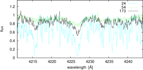
Figure 1: A comparison of a part of the spectrum of the SB2 star 173 (thick black line), the hot star 54 (dotted green line), and the cool star 24 (dashed blue line).

4.1 Stars with variable radial velocity

Our observations of each target star were separated by only one or two nights, which is not optimal for detecting $RV$ variability. Indeed, we only measure $RV$ changes for two stars: 173 and 489. Star 173, which we discover to be a double-lined spectroscopic binary (SB2), shows spectral features of a hot star superimposed on the spectrum of a cool star. This is shown in Fig. 1, where we plot a part of the spectra for stars 173, 24 (a cool star), and 54 (a hot star). The $RV$ values of the A and B components of star 173 measured on 10 and 11 August 2008 are similar, which is consistent with the  1-day period shown by this star in the Kepler photometry (Uytterhoeven et al., 2011).

For star 489, we discovered significant changes in $RV$. Furthermore, both our measured values, $-2.06\pm 0.44$ and $+5.74\pm 0.60$ km s^-1, differ from the $RV$ value reported by Frinchaboy & Majewski (2008) of $+20.01\pm 2.54$ km s^-1, which suggests that star 489 is a spectroscopic binary. Indeed, its spectral lines show a slight asymmetry, but that may be caused either by another star, making star 489 an SB2 system, or by star spots or other surface variations such as pulsations. The latter possibility is very probable because the star is a $\delta$ Sct-type variable (Van Cauteren et al., 2005). Therefore, we caution the reader not to put to much trust in our spectroscopic results derived for star 489 under the assumption of a single star. A similar caution should be adopted also for the other hot, fast-rotating stars in our sample (see Sect. 5.2.2 and Table 5).

For the four stars described below, the spectroscopic binarity was either already known, or has been discovered by comparing our $RV$ measurements with those available in the literature (see Fig. 2).

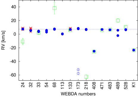
Figure 2: Blue dots indicate $RV$ values of single stars, SB1 systems, and star 173 A from Table 1. Blue open circles indicate the $RV$ values of star 173 B; green squares are the $RV$ values of stars observed by Frinchaboy & Majewski (2008), and red crosses are $RV$ values of stars observed by Mermilliod, Mayor & Udry (2008). The dashed line indicates the mean $RV$ of NGC 6811, $+6.68$ km s^-1, as derived in this paper.

Star 24 has $RV$-values which are constant within the $1\sigma$ error-bars in our observations and they are consistent with the nine $RV$ values reported by Mermilliod, Mayor & Udry (2008). However, they differ from the single $RV$ measurement obtained by Frinchaboy & Majewski (2008), $-10.71\pm 4.80$ km s^-1. The observations by Mermilliod, Mayor & Udry (2008) cover a time-span of 18 years. During that period, the radial velocity of star 24 has never fallen outside the range from $+6.68\pm 0.45$ to $+8.97\pm 0.80$ km s^-1. Therefore, the measurement reported by Frinchaboy & Majewski (2008) is unexpected. We classify star 24 as a suspected single-lined spectroscopic binary (SB1?).

Star 32 has been discovered as a spectroscopic binary by Mermilliod & Mayor (1990). The $RV$ values derived here, $+5.20\pm 0.41$ and $+5.37\pm 0.49$ km s^-1, fall in the range of the $RV$-values reported by Mermilliod, Mayor & Udry (2008), which was from $+3.49\pm 0.53$ to $+9.07\pm 0.38$ km s^-1.

Star 68 has been discovered as an eclipsing binary by Watson, Henden & Price (2006) and is listed in the Kepler eclipsing binary catalogue by Prs̆a et al. (2011). The Kepler light curve of this star reveals a contact system with partial eclipses of similar, but not identical, depths. Because of the near equal depth of the eclipses, one would expect star 68 as an SB2 system. However, our spectra are separated in time by about half an orbital period, which amounts to 4.41599 days (Prs̆a et al., 2011), and show only one component with a high rotational velocity. We expect that this is due to an unfortunate timing of our observations, which happens to coincide with the times of eclipses and the corresponding $RV$ crossing of the binary components. Further observations could confirm this. The $RV$ value reported for this target by Frinchaboy & Majewski (2008), $+38.18\pm 8.89$ km s^-1, is significantly higher than the $RV$ values measured here. However, the fact that our observations most likely include the combined spectra of two fast rotating components, one of which is partially eclipsed, makes a spectroscopic analysis very difficult.

Star 218 does not show $RV$ variability in our observations ($RV=+6.56\pm 1.46$ and $+7.08\pm 1.51$ km s^-1), but the $RV$ value reported by Frinchaboy & Majewski (2008) of $-62.54\pm 3.17$ km s^-1 is significantly different from our measurements. This star has been classified as a $\delta$-Sct-type variable by Debosscher et al. (2011), but an amplitude equal to almost 70 km s^-1 is too high to be caused only by pulsations. We classify star 218 as a single-lined spectroscopic binary.

The stars classified as spectroscopic binaries in this paper are indicated as such in the last column of Table 1.

4.2 Cluster membership

The large amount of spectroscopic binaries in our sample makes it difficult, from our data, to determine if the stars are cluster members. Stars which are not known or suspected spectroscopic binaries, and which have $RV$ values in the range from 6 to 9 km s^-1 to within $3\sigma$, are classified as certain cluster members. This range is based on the determinations of the mean radial velocity of the cluster, as obtained by other authors. These range from $+6.03\pm 0.30$ km s^-1 by Frinchaboy & Majewski (2008) to $+8.7$ km s^-1 by Wong & Meibom (2009).

This approach allowed us to classify stars 33, 54, 133, 471, 483, and 528 as cluster members. Stars 24 and 32 are classified as very probable cluster members. Star 32 is a known, and star 24 a suspected, spectroscopic binary. However, both stars have been classified as certain cluster members based on their proper motions, their radial velocities, and their photometric and seismic properties by other authors (see Sanders, 1971; Mermilliod & Mayor, 1990; Dias, Lepine & Alessi, 2002; Stello et al., 2011).

Stars 173, 408 and K1 are classified in the present paper as non-members because their radial-velocities are significantly different from the cluster mean value. In the case of the SB2 star 173, we made use of the fact that the $RV$ of the A component is very close to the mean $RV$ of the cluster, derived in the previous studies, while the $RV$ of the B component is at around $-52$ km s^-1. This leads to the conclusion that the systemic velocity must be different from the mean velocity of NGC 6811, thus the stellar system does not belong to cluster.

For the SB2 star 68 and the three $\delta$ Sct-type variables, stars 113, 218 and 489, membership have not been assessed. All these stars require more observations in order to determine their mean radial velocity and draw conclusions on their membership to the cluster.

The membership status of our target stars to NGC 6811 is given in Table 1. The six stars classified as members are indicated with ’yes’, the two very probable members with ’yes?’, the three non-members with ’no’, and the four stars without membership classification with a question mark. In Fig. 3, we show the colour-magnitude diagram of the cluster with the positions of our targets indicated. The colour-magnitude diagram is based on $J$ and $K_{S}$ magnitudes adopted from the 2MASS catalogue (Cutri et al., 2003). The $J$ and $K_{S}$ magnitudes of our programme stars are reproduced in columns 6 and 7 in Table 1.

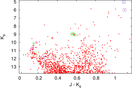
Figure 3: Colour-magnitude diagram based on stars within a radius of $r=20$ arcmin from the centre of the open cluster NGC 6811. The symbols indicate, for our targets, certain and the very probable members of the cluster (circles), non-members (squares), and the stars for which membership is uncertain (triangles). The remaining stars are plotted with dots.

4.3 Mean radial-velocity of the cluster

The first determination of the mean radial-velocity of NGC 6811 was provided by Mermilliod & Mayor (1990) who used the CORAVEL spectrovelocimeters to acquire from three to six spectrograms of stars 24, 32, 73, 79, 101, 133, 210, 223, 234, and 237. Those stars were classified as probable cluster members by Sanders (1971) who analysed proper motions of 296 stars in the field of NGC 6811 and concluded that 97 of the stars most probably belong to the cluster. Mermilliod & Mayor (1990) confirmed the cluster membership for stars 24, 32, 101, and 133, and derived the mean $RV$ of the cluster, $+7.14\pm 0.26$ km s^-1, using stars 24, 101, and 133. Star 32 was not used because those authors discovered it to be a spectroscopic binary system. Eighteen years later, Mermilliod, Mayor & Udry (2008) re-determined the mean $RV$ of NGC 6811 obtaining the value $+7.28\pm 0.19$ km s^-1 from the same three stars and a more extended set of observations.

A slightly lower value of $+6.05\pm 0.95$ km s^-1 was obtained by Kharchenko et al. (2005) who used literature $RV$ values of two cluster members. That value is close to $+6.03\pm 0.30$ km s^-1 derived by Frinchaboy & Majewski (2008) from single spectrograms of stars 33, 106, 133, 471, 483, TYC 3556-02634-1, and TYC 3556-00370-1 acquired with the WIYN 3.5-m telescope at the Kitt Peak National Observatory.

The most recent determination of the mean radial-velocity of NGC 6811, $+8.7$ km s^-1, has been reported by Wong & Meibom (2009) who observed 1157 stars in the field of the cluster with the Hectochelle spectrograph at the Multiple Mirror Telescope and classified 139 of them as candidate cluster members.

In this paper, we derive the radial velocity of NGC 6811 to be $+6.68\pm 0.08$ km s^-1, by computing a weighted mean of the $RV$s of stars 133, 471, 483, and 528 which are neither known nor suspected spectroscopic binaries, and which are classified in this paper as cluster members. In the calculations, we did not include stars 33 and 54, because these are fast rotators causing less precise $RV$ values and, for the hot stars, our evaluation of whether the spectra contain spectral lines from a second component is less certain.

5 Atmospheric Parameters

5.1 Methods

We use three independent methods of spectroscopic analysis for deriving atmospheric parameters and projected rotational velocities of our target stars. These are implemented in the codes FITSUN, SME, and ROTFIT which adopts different approaches for deriving $T_{\rm eff}$, $\log g$, [Fe/H], and $v\sin i$. Each of these methods as suffers from different limitations, as described below. The purpose of choosing these three significantly different methods was to benefit from diversification of approaches in order to evaluate the overall uncertainties in the results as outlined by, e.g., Smalley (in prep.).

5.1.1 ROTFIT

The ROTFIT code has been developed by Frasca et al. (2003, 2006) to perform an automatic classification of the spectral type and the luminosity class, and to derive the projected rotational velocity of late-type stars. Subsequently, the method was developed to allow simultaneous determination of $T_{\rm eff}$, $\log g$, $\rm[Fe/H]$, $v\sin i$, and the MK type of those stars.

One of the advantages of ROTFIT is that, unlike other methods of spectroscopic analysis, it can be applied also to spectra of low resolution, low signal-to-noise ratio, and $v\sin i$ exceeding 20 km s^-1. The properties and limitations of ROTFIT have been described and discussed in detail by Molenda-Żakowicz et al. (2013). Briefly, the method consists in comparing spectra of the programme stars with a library of spectra of the reference stars. The latter, consisting of 221 stars listed by Molenda-Żakowicz et al. (2013), was constructed from the high-resolution ($R=42,000$), high signal-to-noise spectra of slowly rotating stars from the ELODIE archive (Prugniel & Soubiran, 2001) for which the atmospheric parameters are measured with relatively high accuracy.

The uncertainties of $T_{\rm eff}$, $\log g$, $\rm[Fe/H]$, and $v\sin i$ are the standard errors of the respective weighted means to which the average uncertainties of the stellar parameters of the reference stars, i.e. $\sigma_{T_{\rm eff}}=88$ K, $\sigma_{\log g}=0.21$ dex, and $\sigma_{\rm[Fe/H]}=0.21$ dex, are added in quadrature (see Molenda-Żakowicz et al., 2013).

5.1.2 FITSUN

In this method, spectral synthesis based on the least squares optimisation algorithm are used to determine the atmospheric parameters, the projected rotational velocity and radial velocity of stars. To perform the spectrum analysis, a pre-computed grid of atmospheric models is necessary. For the stars analysed in this paper, we derived the line-blanketed LTE models by using the code ATLAS9 by Kurucz (1993). The grid covered the range in $T_{\rm eff}$ from 4750 to 6000 K with a step of 50 K and from 6000 to 9000 K with a step of 100 K. The range in $\log g$ is from 2.70 to 4.50 dex with a step of 0.10 dex. The grid has been computed for solar metallicity with the abundances of elements from Grevesse & Sauval (1998). The spectrum synthesis code FITSUN uses the SYNTHE suite of programs by Kurucz (1993) which allow to compute synthetic spectra. Both ATLAS9 and SYNTHE have been ported under GNU Linux by Sbordone (2005) and are available online.

The detailed description of the method and the performance of the code FITSUN has been provided by Niemczura, Morel & Aerts (2009). This method allows for deriving atmospheric parameters of stars by carrying out spectral synthesis for spectral features chosen according to the spectral type of the target. The line list by Kurucz is used. We start by examining the observed spectrum and adopting an initial set of atmospheric parameters of the targets, either by visual inspection of selected lines in their spectra (F-type stars) or by adopting the values derived by means of other methods (i.e. the code ROTFIT). Then, we build a dense grid of atmosphere models, large enough to cover the expected range of the atmospheric parameters for our targets. Before running the code FITSUN, the observed spectra must be prepared for the analysis. This includes normalisation to the level of continuum, deciding which spectral features will be considered for analysis and dividing the spectrum into parts. The length of those parts depends mainly on the values of $v\sin i$ of the star. Then, FITSUN makes use of SYNTHE and the adopted atmosphere model to calculate the synthetic spectrum in the selected parts, and uses the least-squares method to calculate the abundances of elements, the radial velocity, and the projected rotational velocity of the targets, as described by Niemczura, Morel & Aerts (2009). If necessary, FITSUN corrects on-the-fly the continuum placement of the selected parts of spectra. The eventual usefulness of this method depends on the projected rotational velocity of the star and the correct continuum placement.

5.1.3 SME

The package Spectroscopy Made Easy (SME) by Valenti & Piskunov (1996) is an IDL program which allows to fit the observed spectrum with a synthetic one and to determine the atmospheric parameters of the programme star. In SME, the spectrum synthesis and the $\chi^{2}$-minimisation in the spectral regions defined by the input masks are carried out on-the-fly. In these computations, we used the MARCS model atmospheres by Gustafsson et al. (2008). When defining the masks, we selected only those iron lines for which the complete NLTE grids of abundance corrections are available. In total, we used about 60 diagnostic Fe I and Fe II transitions. The line list was built from the SIU line list which is a compilation by different groups (Korn et al., 2003; Grupp, 2004a, b; Bergemann & Gehren, 2008; Bergemann & Cescutti, 2010; Bergemann et al., 2012a, b; Önehag et al., 2011; Shi et al., 2014) and applied in different spectroscopic studies (see, e.g. Bergemann, 2011). The stellar parameters were determined iteratively, exploring the full parameter-space in $T_{\rm eff}$, $\log g$, [Fe/H], the micro-turbulence velocity ($\xi_{\rm t}$) and the macro-turbulence velocity ($v_{\rm mac}$). The influence of NLTE effects was treated using the model atom and the grids presented by Bergemann et al. (2012c); Lind et al. (2012).

The uncertainties of the stellar parameters produced by SME are combined estimates stemming from several sources. First, SME accounts for the signal-to-noise of a spectrum while iteratively searching for the most probable solution in the full parameter space. The robustness of the final values of the parameters is assessed by perturbing the initial guesses and reiterating until convergence. These are the internal uncertainties of the method. Second, we include systematic errors which have been determined from the analysis of a reference high-resolution stellar sample (see Bergemann et al., 2012c, Bergemann et al., in prep.) for which the parameters obtained by independent methods such as interferometry and asteroseismology are available. The mean difference between those values and the results produced by SME are adopted for a measure of the systematic error for a given spectral type. The individual uncertainties are combined in quadrature and their maximum is adopted as the final uncertainty of the parameter under consideration.

5.2 Results

The atmospheric parameters obtained by means of the three methods described in Section 5.1 are discussed below, separately for the F-, G-, and M-type stars. For each star and each method, the values which we report are means calculated from the results obtained from two individual spectra.

5.2.1 G-type stars

Table 2: Seismic parameters of G-type stars.

WEBDA (KIC)	$\Delta\nu\pm\sigma$	$\nu_{\rm max}\pm\sigma$	$\log g_{\rm seis.}$
	[$\mu$Hz]	[$\mu$Hz]	[dex]
24 (9655101)	7.86$\pm$0.04	98.2$\pm$2.4	2.90
32 (9655167)	8.07$\pm$0.04	100.3$\pm$8.7	2.91
133 (9716090)	8.56$\pm$0.06	101.4$\pm$5.9	2.92
471 (9776739)	7.93$\pm$0.16	93.4$\pm$9.0	2.88
483 (9532903)	7.69$\pm$0.16	96.3$\pm$4.5	2.90

The G-type stars 24, 32, 133, 471, and 483 observed by us in the field of NGC 6811 form a small, distinct group located at $K_{S}\simeq 9$ mag, $(J-K_{S})\simeq 0.6$ mag in the colour-magnitude diagram shown in Fig. 3. Stars 24, 32, and 133, have been classified as red clump (RC) by Mermilliod & Mayor (1990) who inferred that from the colour-magnitude diagram of the cluster. This classification was then confirmed by Corsaro et al. (2012) who analysed the asteroseismic properties of these stars. Our analysis shows that also stars 471 and 483 should be classified as RC. They are cluster members (see Sect. 4.2) and they fall in the same region of the $K_{S}-(J-K_{S})$ diagram as stars 24, 32, and 133 (see Fig. 3). Moreover, they have very similar values of the atmospheric parameters as the three other RC stars (see Table 3). Unfortunately, neither star 471 nor 483 was included in the sample analysed by Corsaro et al. (2012).

However, all five stars show solar-like oscillations which was discovered in the Kepler data by Hekker et al. (2011) and Stello et al. (2011). As showed in Table 2, the asteroseismic parameters of these stars are very similar which further indicates that they are all RC-stars. We have computed asteroseismic values of $\log g$ for these five stars, in order to check the accuracy of our spectroscopic values $\log g$ values. We made use of the fact that the asteroseismic values of $\log g$ are not only precise but also accurate, at least at metallicities close to and higher than solar, even if the mass derived from the asteroseismic scaling relations seems to be slightly overestimated (see Brogaard et al., 2012; Sandquist et al., 2013; Frandsen et al., 2013). We used the asteroseismic parameters derived for stars 24, 32 and 133 by Corsaro et al. (2012), and for stars 471 and 483 by Hekker et al. (2011), kindly provided to us by the first authors of those two papers. We reproduce these parameters in Table 2 where the symbols $\Delta\nu$ and $\nu_{\rm max}$ stand for the large separation between consecutive overtones and the frequency of maximum power of the oscillations, respectively (see, e.g., Stello et al., 2009). We note that the differences between uncertainties of those values reported by Hekker et al. (2011) and Corsaro et al. (2012) result from the different lengths of the time-series analysed by these two groups (nearly a year by Hekker et al. (2011) and more than 19 months by Corsaro et al. (2012)). In the computations, we used the asteroseismic scaling relations for mass and radius (eqns. 3 and 4 from Miglio et al., 2012) and the values of $T_{\rm eff}$ derived with FITSUN (Table 3). In principle, the spectroscopic analysis should be iterated after using the derived values of $T_{\rm eff}$ to calculate new asteroseismic values of $\log g$. However, since changes to the values of $\log g$ were already less than 0.01 dex in the first iteration, further iterations were not needed. The resulting values of $\log g_{\rm seism.}$ are provided in the fourth column of Table 2. A conservative uncertainty estimate for these values is $\pm 0.04$ dex.

Table 3: Atmospheric parameters of G-type stars; the uncertainties of the derived values are given in the text.

FITSUN
WEBDA (KIC)	$T_{\rm eff}$	$\log g$	$\rm[Fe/H]$	$v\sin i$	$\xi_{\rm t}$	$T_{\rm eff}$	$\log g_{\rm seis.}$	$\rm[Fe/H]$	$v\sin i$	$\xi_{\rm t}$
	[K]	[dex]	[dex]	[km s-1]	[km s-1]	[K]	[dex]	[dex]	[km s-1]	[km s-1]
	$\log g$ free					$\log g_{\rm seis.}$ fixed
24 (9655101)	5050	3.00	0.06	4.8	1.00	5000	2.90	0.00	4.8	1.10
32 (9655167)	5050	2.90	0.09	5.1	1.10	5050	2.91	0.09	5.1	1.10
133 (9716090)	5100	2.90	0.07	4.5	1.10	5100	2.92	0.07	4.5	1.10
471 (9776739)	4950	2.90	0.04	4.7	1.10	4950	2.88	0.04	4.7	1.10
483 (9532903)	—	—	—	—	—	5050	2.90	0.04	4.7	1.10
SME
WEBDA (KIC)	$T_{\rm eff}$	$\log g$	$\rm[Fe/H]$	$v\sin i$	$\xi_{\rm t}$; $v_{\rm mac}$	$T_{\rm eff}$	$\log g_{\rm seis.}$	$\rm[Fe/H]$	$v\sin i$	$\xi_{\rm t}$; $v_{\rm mac}$
	[K]	[dex]	[dex]	[km s-1]	[km s-1]	[K]	[dex]	[dex]	[km s-1]	[km s-1]
	$\log g$ free					$\log g_{\rm seis.}$ fixed
24 (9655101)	5083	3.05	0.08	0.1	1.11; 3.85	5005	2.90	0.03	0.1	1.11; 3.85
32 (9655167)	4939	2.95	0.06	4.1	1.11; 3.85	4924	2.91	0.05	4.1	1.11; 3.85
133 (9716090)	5005	2.97	0.05	0.1	1.11; 3.84	4980	2.92	0.02	0.1	1.11; 3.84
471 (9776739)	4922	2.81	0.03	0.1	1.11; 3.87	4952	2.88	0.05	0.1	1.11; 3.87
483 (9532903)	5066	3.02	0.09	0.1	1.11; 3.91	5008	2.90	0.05	0.1	1.11; 3.91
	ROTFIT					Kepler Input Catalog
WEBDA (KIC)	$T_{\rm eff}$	$\log g$	[Fe/H]	$v\sin i$	MK	$T_{\rm eff}$	$\log g$	$\rm[Fe/H]$
	[K]	[dex]	[dex]	[km s-1]	type	[K]	[dex]	[dex]
	$\log g$ free					griz photometry
24 (9655101)	5135	3.18	$-$0.05	0.1	G8 III	5078	2.9	0.05
32 (9655167)	5103	3.17	$-$0.04	0.1	G8 III	5034	2.9	0.00
133 (9716090)	5130	3.20	$-$0.04	0.1	G8 III	5042	2.8	$-$0.10
471 (9776739)	5095	3.11	$-$0.04	0.1	G8 III	5146	2.9	$-$0.09
483 (9532903)	5120	3.21	$-$0.04	0.1	G8 III	5119	2.5	0.06

Below, we present the atmospheric parameters obtained for these five stars independently with the codes FITSUN, SME, and ROTFIT. In case of FITSUN and SME, apart from the purely spectroscopic analysis, we carried out additional computations with $\log g$ fixed to the asteroseismic values from Table 2. In Table 3, where we present the results, the parameters obtained from purely spectroscopic analyses are labelled ’$\log g$ free’ while those obtained for $\log g$ fixed to the asteroseismic value are labelled ’$\log g$ fixed’. Table 3 also provides the photometric values of the atmospheric parameters of our targets reproduced from the KIC.

Table 4: Mean atmospheric parameters of G-type stars and the biases between the methods.

Parameter	FITSUN	SME	ROTFIT	$\Delta_{\tiny\textsc{(FITSUN - SME)}}$	$\Delta_{\tiny\textsc{(FITSUN - ROTFIT)}}$	$\Delta_{\tiny\textsc{(ROTFIT - SME)}}$
$\rm\langle T_{\rm eff}\rangle_{\,\log g\,free}$ [K]	$5038\pm 32$	$5003\pm 32$	$5117\pm 8$	$35\pm 45$	$-79\pm 33$	$114\pm 33$
$\rm\langle\log g\rangle_{\,\log g\,free}$ [dex]	$2.95\pm 0.03$	$2.96\pm 0.04$	$3.17\pm 0.02$	$-0.01\pm 0.05$	$-0.22\pm 0.04$	$0.21\pm 0.05$
$\rm\langle[Fe/H]\rangle_{\,\log g\,free}$ [dex]	$0.07\pm 0.01$	$0.06\pm 0.01$	$-0.04\pm 0.002$	$0.01\pm 0.02$	$0.11\pm 0.01$	$-0.10\pm 0.01$
$\rm\langle T_{\rm eff}\rangle_{\,\log g_{\rm seis.}\,fixed}$ [K]	$5030\pm 25$	$4974\pm 16$	—	$56\pm 30$	—	—
$\rm\langle\log g_{\rm seis.}\rangle$ [dex]	$2.90\pm 0.01$	$2.90\pm 0.01$	—	—	—	—
$\rm\langle[Fe/H]\rangle_{\,\log g_{\rm seis.}\,fixed}$ [dex]	$0.05\pm 0.02$	$0.04\pm 0.01$	—	$0.01\pm 0.02$	—	—

• FITSUN

  The atmospheric parameters obtained with FITSUN are provided in the top part of Table 3. The left side of the Table, labelled ’$\log g$ free’, lists the values of $T_{\rm eff}$, $\log g$, $\rm[Fe/H]$, and $v\sin i$, resulting from a purely spectroscopic analysis. The values of $\rm[Fe/H]$ and $T_{\rm eff}$ have been derived from isolated, unblended lines of Fe I. The right side of Table 3 lists the atmospheric parameters and $v\sin i$ obtained with $\log g$ fixed to the asteroseismic value for which a dedicated grid of model atmospheres has been prepared. In both computations, the value of $v_{\rm mac}$ has been set to zero. For star 483 for which we detected only one useful line of Fe II we present only the atmospheric parameters derived for the fixed, asteroseismic value of $\log g$. The steps in our grid of model atmospheres, i.e. 50 K in $T_{\rm eff}$, 0.1 dex in $\log g$, and 0.5 km s^-1 in $\xi_{t}$, define the uncertainties of these parameters. The typical uncertainty of the value of $\rm[Fe/H]$ is 0.20 dex (c.f. Table 7.) The typical uncertainty of $v\sin i$ is $\pm 1.0$ km s^-1.

• SME

  The NLTE results obtained with the code SME and the grid of NLTE corrections by Lind et al. (2012) are provided in the middle part of Table 3 separately for the free and the fixed values of $\log g$. The values of $\xi_{\rm t}$ and $v_{\rm mac}$ have been obtained from a calibration relation by Bergemann et al., (in prep.) The uncertainties of the computed values are 150 K in $T_{\rm eff}$, 0.15 dex in $\log g$, 0.10 dex in [Fe/H], and 0.5 km s^-1 in and $v\sin i$. The uncertainties for $\xi_{\rm t}$ and $v_{\rm mac}$ have not been provided. Both quantities are ad-hoc parameters introduced to approximate non-thermal broadening and do not have a physical measurable equivalent. In 3D hydrodynamic simulations, turbulent velocity fields are stochastic and do not take a single constant value throughout a stellar atmosphere.

• ROTFIT

  The results obtained with ROTFIT are provided at the bottom left of Table 3. They have been obtained only for the free $\log g$ because ROTFIT does not allow to fix any of the atmospheric parameters (see Frasca et al., 2003, 2006; Molenda-Żakowicz et al., 2013). The standard errors of the obtained atmospheric parameters are 120 K in $T_{\rm eff}$, 0.22 dex in $\log g$ and [Fe/H], and 0.4 km s^-1 in $v\sin i$.

• KIC

  The photometric values of $T_{\rm eff}$, $\log g$, and $\rm[Fe/H]$ from the KIC catalogue have been provided at the bottom right of Table 3. The precision of these parameters is 200 K in $T_{\rm eff}$, and 0.5 dex in $\log g$ and $\rm[Fe/H]$ (Brown et al., 2011).

The values of $T_{\rm eff}$, $\log g$, and $\rm[Fe/H]$ derived for G-type stars by means of the three methods used in this paper agree with each other to within $1\sigma$ error bars. The mean values of $T_{\rm eff}$, $\log g$, and $\rm[Fe/H]$ of G-type stars in NGC 6811, calculated from the individual values from Table 3, are provided in Table 4. The same table provides also biases between FITSUN, SME, and ROTFIT. The uncertainties of the reported values are standard deviations of the mean.

The biases listed in Table 4 show that ROTFIT produced a temperature scale which is higher by around 70 K comparing to FITSUN and around 110 K comparing to SME, while SME produced a temperature scale which is lower by around 30 K comparing to FITSUN. For the fixed values of $\log g$, the last difference amounts to around 70 K.

The mean values of $\log g$ and $\rm[Fe/H]$ produced by FITSUN and SME agree nicely with each other. They are also in a very good agreement with the asteroseismic values of $\log g$. A similarly good agreement between the spectroscopic and asteroseismic values of $\log g$ has been reported by Bruntt et al. (2012) and Thygesen et al. (2012) who used the code VWA (Bruntt et al., 2010) to perform spectroscopic analysis of 93 solar-type stars and 82 red giants, and detected only a handful of outliers. However, one cannot just expect a general good agreement between spectroscopic and asteroseismic $\log g$ values. As a relevant example, quite discordant values of spectroscopic $\log g$ were obtained by Molenda-Żakowicz et al. (2013) with the code ARES+MOOG (Santos, Israelian & Mayor, 2004; Sousa et al., 2006, 2008, 2011a, 2011b) for stars 24, 32, and 133 which are on average 0.5 dex higher than the asteroseismic values reported in this paper. (We note that the values of $\log g$ obtained by Molenda-Żakowicz et al. (2013) with the code ROTFIT agree well with those derived with ROTFIT in this paper.)

Apart from a higher temperature scale, ROTFIT produced also values of $\log g$ which are higher by 0.20-0.25 dex, and values of $\rm[Fe/H]$ which are lower by 0.06-0.10 dex in comparison with the two other methods. The simplest explanation for that is a weak correlation between the fitted parameters $T_{\rm eff}$ and $\log g$ which has a different behaviour depending on the adopted analysis code and, most importantly, on the analysed spectral range. Therefore, it is not surprising that FITSUN and SME which use unblended Fe I and Fe II lines agree better with each other than with ROTFIT which analyses entire spectral segments containing also strong and broad absorption lines. The observed discrepancy may be also due to the grid of templates which, being composed of real star spectra, cannot cover all the regions of the parameter-space with equal density (see figure 2 in Molenda-Żakowicz et al., 2013). On the other hand, we note that the biases reported in Table 4 may be lower or even reversed when ROTFIT is compared to other spectroscopic or photometric methods (see figures 4 and 6 in Molenda-Żakowicz et al., 2013). Therefore, our results support the conclusion of Molenda-Żakowicz et al. (2013) that the present accuracy of determinations of the atmospheric parameters of solar-type stars is not better than $\pm 150$ K in $T_{\rm eff}$, $\pm 0.15$ dex in [Fe/H], and $\pm 0.3$ dex in $\log g$ when no asteroseismic $\log g$ values are available.

When explaining the sources of differences between the results produced by FITSUN and SME, multiple reasons can be indicated (see, e.g., Smalley in prep.). Below, we list the most important ones (the following comparisons does not concern ROTFIT because the latter code uses for an input a grid of atmospheric parameters of reference stars that were computed by various authors and by means of different methods; see Molenda-Żakowicz et al., 2013):

• The choice of model atmospheres: FITSUN uses the plane-parallel LTE model atmospheres by Kurucz while SME uses the spherically-symmetric MARCS model atmospheres;

• The adopted atomic data: FITSUN uses the Kurucz atomic and molecular line list (see Sect. 5.1.2) while SME uses the updated line list from SIU spectrum synthesis code (see Sect. 5.1.3);

• The reference to the solar abundances: FITSUN uses the reference by Grevesse & Sauval (1998) while SME, the reference by Grevesse, Asplund & Sauval (2007) which is the source of a slight difference in solar abundances adopted in the two codes ($\log(\rm Fe)=7.50$ in FITSUN and $\log(\rm Fe)=7.45$ in SME);

• The procedure of deriving the atmospheric parameters: FITSUN uses an iterative approach to derive the atmospheric parameters while SME, which also solves for stellar parameters iteratively, exploring the full parameter space, derives the values of $T_{\rm eff}$, $\log g$, and $\rm[Fe/H]$ simultaneously.

These are accompanied with other, secondary factors which are altogether sufficient to produce noticeable differences between the values of $T_{\rm eff}$, $\log g$, and $\rm[Fe/H]$ derived by means of different methods. As shown by, e.g., Metcalfe et al. (2010); Gómez Maqueo Chew et al. (2013), or and Guzik et al., in prep., such differences for stars similar to the Sun or slightly hotter can easily exceed 100 K in $T_{\rm eff}$ and 0.6 dex in $\log g$ (c.f. the results obtained for stars 24, 32, and 133 by Molenda-Żakowicz et al., 2013).

Since all the G-type stars from Table 3 have been classified in this paper as cluster members, their mean metallicity $\langle\rm[Fe/H]\rangle$ can be adopted for the mean metallicity of the cluster. These mean values, calculated separately for each method, are provided in Table 4. They range from $-0.04\pm 0.002$ dex obtained with ROTFIT to $0.06\pm 0.01$ dex obtained with SME from the fully spectroscopic analysis, i.e. the ’$\log g$ free’ case. These values agree with what is expected for a Galactic open cluster located at the galactocentric radius $R_{\rm GC}=8.3$ kpc and an age of about 1 Gyr (see Sect. 7 and figures 9 and 10 in Pancino et al., 2010). Previous determinations of $\rm[Fe/H]$ of NGC 6811 were lower. They ranged from $-0.1$ dex, derived by Wong & Meibom (2009) from observations acquired with the Hectochelle spectrograph on the Multiple Mirror Telescope, through $-0.19$ dex, derived by Janes et al. (2013) from photometric observations and fitting isochrones to the cluster colour-magnitude diagram, to a value as low as $\rm-0.3>[Fe/H]>-0.7$ dex, as proposed by Hekker et al. (2011) from an analysis of the position of four cluster red giants in the $\log T_{\rm eff}$–$\log L$ diagram. Neither the results obtained in this paper nor those reported by Molenda-Żakowicz et al. (2013) confirm such a low metallicity of NGC 6811. In Sect. 7, we provide explanations for the deviating results of Hekker et al. (2011) and Janes et al. (2013).

All our codes find the G-type stars to be slow rotators. FITSUN finds the values of $v\sin i$ of our targets to fall in the range from 3.7 to 4.4 km s^-1. This range is confirmed by SME only for star 32; the remaining stars are found by that code to have $v\sin i=0.1$ km s^-1. The difference in $v\sin i$ as derived by FITSUN and SME is caused by the different assumptions on $v_{\rm mac}$. Also ROTFIT yields $v\sin i=0.1$ km s^-1 for all the five stars but in that case, the values of $v\sin i$ may be underestimated; when computing $v\sin i$, ROTFIT assumes that the reference stars do not rotate while in reality they do. However, at the resolution of our spectra (R=25,000) ROTFIT can neither easily resolve the effect of $v_{\rm mac}$ and $v\sin i$ on the line profiles nor measure any broadening effect smaller than around 5 km s^-1. Therefore, we conclude that the values of $v\sin i$ obtained with the three methods are consistent with each other.

5.2.2 F-type stars

In the case of fast rotating F-type stars, to derive $T_{\rm eff}$ and $\log g$, we used the Balmer lines, and we required the same abundances from all available Fe I and Fe II lines. Since we had low signal-to-noise spectra of fast rotating stars at our disposal, we did not detect the weak, unblended lines of iron which is why the determination of accurate values of $\xi_{\rm t}$ and $\log g$ was impossible. Therefore, we decided to fix the value of $\xi_{\rm t}$ to 3 or 4 km s^-1, depending on the resulting [Fe/H] which we tried to keep as close as possible to the mean value of [Fe/H] of G-type stars derived with FITSUN, derive only the values of $T_{\rm eff}$, and estimate the values of $\log g$. For each of the stars the last parameter was falling in the range from 3.5 to 4.0 dex with the uncertainty of 0.4 dex, and with little influence on the eventual values of $T_{\rm eff}$.

The results of this analysis are presented in Table 5. The uncertainty of the values of $T_{\rm eff}$ is 100 K. The uncertainties of the values of $v\sin i$ are provided in the Table. Table 5 lists also the values of $T_{\rm eff}$ from the KIC which are available for three of our targets and which agree with our determinations to within $1\sigma$ error bars.

We do not provide the results of the analyses carried out with SME and ROTFIT because for the former code, the spectra were of too low quality while for the latter one, the stars fall too close to the limits in $T_{\rm eff}$ of the grid of the reference stars (see Molenda-Żakowicz et al., 2013).

Table 5: Atmospheric parameters of F-type stars.

	FITSUN
WEBDA (KIC)	$T_{\rm eff}$	$v\sin i$	$T_{\rm eff,KIC}$
	[K]	[km s-1]	[K]
33 (9716220)	7600	172 $\pm$ 20	7725
54 (9655438)	7100	222 $\pm$ 16	6974
113 (9655514)	7400	101 $\pm$   9	7441
218 (9716667)	7600	167 $\pm$ 24	—
489 (9594857)	7000	94 $\pm$   9	—
528 (9777532)	7300	65 $\pm$   6	—

Table 6: Atmospheric parameters of M-type stars.

	ROTFIT
WEBDA (KIC)	$T_{\rm eff}$	$\log g$	[Fe/H]	$v\sin i$	SpT
	[K]	[dex]	[dex]	[km s-1]
408 (9715189)	3891	1.75	$-$0.03	0.1	M1 III
K1 (9895798)	3868	1.71	$-$0.06	6.1	M1 III
	Kepler Input Catalog
WEBDA (KIC)	$T_{\rm eff}$	$\log g$	[Fe/H]
	[K]	[dex]	[dex]
K1 (9895798)	3356	0.5	0.58

Figure 4: Part of spectra of two ROTFIT reference stars HD 168720 (M1 III) and GJ 273 (M3.5 V), and the programme stars 408, and K1.

5.2.3 M-type stars

The M-type stars 408 and K1, which are not cluster members, were analysed with the code ROTFIT. The values of $T_{\rm eff}$, $\log g$, $\rm[Fe/H]$, $v\sin i$, and the MK type obtained for them are provided in Table 6. The uncertainties of the derived atmospheric parameters are 100 K in $T_{\rm eff}$, 0.22 dex in $\log g$ and [Fe/H], and 0.8 km s^-1 in $v\sin i$. However, since the two stars fall close to the edge of the grid of parameters of the reference stars used in ROTFIT, (c.f. figure 3 in Molenda-Żakowicz et al., 2013), our determinations may be less accurate than the formal errors.

The KIC catalogue gives the photometric values of $T_{\rm eff}$, $\log g$, and [Fe/H] only for star K1 which is found there to be significantly cooler, more evolved, and metal-rich (see Table 6.) Our analysis does not confirm these values, particularly the value of $T_{\rm eff}$ (we do not discuss the other parameters because our grid of reference spectra contains only a few cool, low-gravity, metal-rich stars.) In order to illustrate the difference between the spectrum of a star of $T_{\rm eff}=3900$ and a star of $T_{\rm eff}=3400$ K, we plot part of the spectra of stars 408 and K1, and the spectra of two ROTFIT reference stars HD 168720 ($T_{\rm eff}=3810$ K, M1 III, Valdes et al., 2004) and GJ 273 ($T_{\rm eff}=3420$ K, M3.5 V, Cesetti et al., 2013) in Fig. 4. Even a visual comparison of these spectra allows to conclude that star K1 can not be as cool as 3350 K which proves that the value of $T_{\rm eff}$ in the KIC is erroneous.

We do not provide the atmospheric parameters derived for star 408 and K1 with FITSUN and SME, because the spectral lines of both of these were severely blended with molecular bands and are therefore not suitable for these two codes.

6 Abundance analysis

Table 7: Chemical abundances of the G-type red clump stars in NGC 6811.

El.	WEBDA (KIC)										Sun
	24		32		133		471		483
	(9655101)		(9655167)		(9716090)		(9776739)		(9532903)
${}_{3}\rm Li$	$1.34$	[1]	$1.46$	[1]	$1.37$	[1]	$1.12$	[1]	$1.27$	[1]	$1.10\pm 0.10$
${}_{11}\rm Na$	$6.45\pm 0.16$	[5]	$6.43\pm 0.06$	[3]	$6.51\pm 0.25$	[8]	$6.33\pm 0.06$	[5]	$6.46\pm 0.14$	[5]	$6.33\pm 0.03$
${}_{12}\rm Mg$	$7.60\pm 0.22$	[10]	$7.61\pm 0.12$	[3]	$7.69\pm 0.11$	[4]	$7.32\pm 0.11$	[8]	$7.59\pm 0.29$	[4]	$7.58\pm 0.05$
${}_{13}\rm Al$	$6.12$	[1]	$6.49$	[1]	$6.18$	[1]	$6.63$	[1]	—		$6.43\pm 0.07$
${}_{14}\rm Si$	$7.41\pm 0.36$	[49]	$7.50\pm 0.34$	[40]	$7.23\pm 0.29$	[40]	$7.23\pm 0.36$	[45]	$7.33\pm 0.26$	[43]	$7.55\pm 0.05$
${}_{16}\rm S$	$7.33$	[2]	$7.55$	[2]	—		—		—		$7.33\pm 0.11$
${}_{20}\rm Ca$	$6.38\pm 0.27$	[35]	$6.48\pm 0.24$	[19]	$6.50\pm 0.21$	[21]	$6.36\pm 0.22$	[23]	$6.23\pm 0.26$	[23]	$6.36\pm 0.02$
${}_{21}\rm Sc$	$3.06\pm 0.33$	[28]	$3.07\pm 0.26$	[21]	$3.08\pm 0.15$	[14]	$3.00\pm 0.22$	[17]	$3.00\pm 0.14$	[19]	$3.17\pm 0.10$
${}_{22}\rm Ti$	$4.93\pm 0.27$	[142]	$4.91\pm 0.26$	[111]	$4.95\pm 0.27$	[115]	$4.85\pm 0.18$	[124]	$4.88\pm 0.18$	[102]	$5.02\pm 0.06$
${}_{23}\rm V$	$3.85\pm 0.28$	[67]	$3.92\pm 0.18$	[47]	$3.93\pm 0.17$	[55]	$3.80\pm 0.22$	[63]	$3.85\pm 0.20$	[51]	$4.00\pm 0.02$
${}_{24}\rm Cr$	$5.67\pm 0.19$	[110]	$5.71\pm 0.19$	[79]	$5.67\pm 0.17$	[87]	$5.65\pm 0.23$	[102]	$5.65\pm 0.22$	[100]	$5.67\pm 0.03$
${}_{25}\rm Mn$	$5.30\pm 0.31$	[43]	$5.38\pm 0.23$	[32]	$5.34\pm 0.28$	[41]	$5.35\pm 0.23$	[41]	$5.35\pm 0.23$	[38]	$5.39\pm 0.03$
${}_{26}\rm Fe$	$7.51\pm 0.17$	[369]	$7.54\pm 0.16$	[191]	$7.58\pm 0.14$	[258]	$7.51\pm 0.15$	[298]	$7.51\pm 0.14$	[316]	$7.50\pm 0.05$
${}_{26}\rm Fe\,I$	$7.56\pm 0.22$	[95]	$7.59\pm 0.19$	[94]	$7.57\pm 0.22$	[117]	$7.54\pm 0.23$	[89]	$7.54\pm 0.19$	[88]
${}_{26}\rm Fe\,II$	$7.56\pm 0.17$	[6]	$7.60$	[2]	$7.57\pm 0.10$	[3]	$7.53\pm 0.29$	[6]	$7.51$	[1]
${}_{27}\rm Co$	$4.86\pm 0.21$	[65]	$4.85\pm 0.19$	[41]	$4.88\pm 0.22$	[44]	$4.79\pm 0.25$	[58]	$4.82\pm 0.25$	[62]	$4.92\pm 0.04$
${}_{28}\rm Ni$	$6.22\pm 0.22$	[115]	$6.27\pm 0.19$	[96]	$6.22\pm 0.23$	[112]	$6.25\pm 0.22$	[111]	$6.20\pm 0.20$	[108]	$6.25\pm 0.04$
${}_{29}\rm Cu$	$4.35\pm 0.22$	[3]	$4.42$	[2]	$4.38$	[2]	$4.34\pm 0.36$	[3]	$4.37\pm 0.56$	[3]	$4.21\pm 0.04$
${}_{30}\rm Zn$	$4.81$	[1]	—		$4.37$	[1]	$4.72$	[1]	—		$4.56\pm 0.08$
${}_{38}\rm Sr$	$3.67$	[1]	—		$3.50\pm 0.13$	[3]	$3.38\pm 0.32$	[3]	$3.58$	[2]	$2.97\pm 0.05$
${}_{39}\rm Y$	$2.45\pm 0.18$	[13]	$2.36\pm 0.15$	[8]	$2.33\pm 0.17$	[8]	$2.32\pm 0.25$	[18]	$2.31\pm 0.19$	[15]	$2.24\pm 0.03$
${}_{40}\rm Zr$	$2.71\pm 0.24$	[13]	$2.24\pm 0.23$	[10]	$2.65\pm 0.37$	[7]	$2.25\pm 0.34$	[13]	$2.41\pm 0.26$	[6]	$2.60\pm 0.02$
${}_{41}\rm Nb$	$1.66$	[1]	—		$1.65$	[1]	—		—		$1.38\pm 0.06$
${}_{42}\rm Mo$	$2.11$	[2]	$2.21$	[2]	$2.18$	[1]	$2.08$	[1]	$2.13$	[1]	$1.92\pm 0.05$
${}_{44}\rm Ru$	—		$1.71$	[1]	—		$1.73$	[2]	$1.82$	[1]	$1.84\pm 0.07$
${}_{56}\rm Ba$	$2.90\pm 0.22$	[5]	$2.94$	[2]	$2.89$	[2]	$2.92\pm 0.04$	[3]	$2.84$	[2]	$2.13\pm 0.05$
${}_{57}\rm La$	$1.50\pm 0.20$	[15]	$1.42\pm 0.07$	[8]	$1.56\pm 0.19$	[6]	$1.43\pm 0.29$	[11]	$1.36\pm 0.15$	[8]	$1.17\pm 0.07$
${}_{58}\rm Ce$	$1.89\pm 0.32$	[20]	$2.22\pm 0.34$	[10]	$1.78\pm 0.33$	[10]	$2.12\pm 0.25$	[18]	$1.88\pm 0.20$	[12]	$1.58\pm 0.09$
${}_{59}\rm Pr$	$1.04\pm 0.47$	[8]	$1.03\pm 0.11$	[4]	—		$0.81\pm 0.36$	[8]	$0.52\pm 0.18$	[5]	$0.71\pm 0.08$
${}_{60}\rm Nd$	$1.65\pm 0.30$	[39]	$1.63\pm 0.24$	[20]	$1.64\pm 0.22$	[29]	$1.69\pm 0.21$	[39]	$1.60\pm 0.22$	[27]	$1.50\pm 0.06$
${}_{62}\rm Sm$	$1.88\pm 0.63$	[5]	—		$1.81\pm 0.32$	[3]	$1.68\pm 0.21$	[7]	$1.49$	[2]	$1.01\pm 0.06$
${}_{64}\rm Gd$	$1.15$	[2]	—		—		—		—		$1.12\pm 0.04$
${}_{66}\rm Dy$	$1.08$	[1]	—		$1.25$	[2]	—		—		$1.10\pm 0.08$

Table 8: The ratios of the abundances of elements to iron for the G-type red clump stars in NGC 6811.

[X/Fe]	WEBDA (KIC)
	24 (9655101)	32 (9655167)	133 (9716090)	471 (9776739)	483 (9532903)	cluster mean
$\rm[Li/Fe]$	$0.18$	$0.27$	$0.20$	$-0.02$	$0.13$	$0.15\pm 0.10$
$\rm[Na/Fe]$	$0.06\pm 0.28$	$0.01\pm 0.21$	$0.11\pm 0.34$	$-0.04\pm 0.24$	$0.09\pm 0.24$	$0.04\pm 0.11$
$\rm[Mg/Fe]$	$-0.04\pm 0.32$	$-0.06\pm 0.24$	$0.04\pm 0.26$	$-0.30\pm 0.26$	$-0.03\pm 0.35$	$-0.09\pm 0.12$
$\rm[Al/Fe]$	$-0.37$	$-0.03$	$-0.32$	$0.16$	—	$-0.14\pm 0.22$
$\rm[Si/Fe]$	$-0.20\pm 0.43$	$-0.14\pm 0.40$	$-0.39\pm 0.37$	$-0.36\pm 0.43$	$-0.26\pm 0.33$	$-0.27\pm 0.17$
$\rm[S/Fe]$	$-0.06$	$0.13$	—	—	—	$0.03\pm 0.09$
$\rm[Ca/Fe]$	$-0.04\pm 0.35$	$0.03\pm 0.31$	$0.07\pm 0.31$	$-0.04\pm 0.32$	$-0.17\pm 0.33$	$-0.03\pm 0.14$
$\rm[Sc/Fe]$	$-0.17\pm 0.41$	$-0.19\pm 0.34$	$-0.16\pm 0.29$	$-0.21\pm 0.34$	$-0.21\pm 0.26$	$-0.19\pm 0.14$
$\rm[Ti/Fe]$	$-0.15\pm 0.36$	$-0.20\pm 0.33$	$-0.14\pm 0.36$	$-0.21\pm 0.30$	$-0.18\pm 0.27$	$-0.18\pm 0.14$
$\rm[V/Fe]$	$-0.21\pm 0.36$	$-0.17\pm 0.27$	$-0.14\pm 0.28$	$-0.24\pm 0.32$	$-0.19\pm 0.28$	$-0.19\pm 0.13$
$\rm[Cr/Fe]$	$-0.06\pm 0.30$	$-0.05\pm 0.27$	$-0.07\pm 0.28$	$-0.06\pm 0.33$	$-0.06\pm 0.30$	$-0.06\pm 0.13$
$\rm[Mn/Fe]$	$-0.15\pm 0.38$	$-0.10\pm 0.30$	$-0.12\pm 0.36$	$-0.08\pm 0.33$	$-0.08\pm 0.30$	$-0.10\pm 0.15$
$\rm[Co/Fe]$	$-0.12\pm 0.31$	$-0.16\pm 0.28$	$-0.11\pm 0.32$	$-0.17\pm 0.35$	$-0.14\pm 0.32$	$-0.14\pm 0.14$
$\rm[Ni/Fe]$	$-0.09\pm 0.32$	$-0.07\pm 0.28$	$-0.10\pm 0.32$	$-0.04\pm 0.32$	$-0.09\pm 0.28$	$-0.08\pm 0.14$
$\rm[Cu/Fe]$	$0.08\pm 0.32$	$0.12$	$0.10$	$0.09\pm 0.43$	$0.12\pm 0.59$	$0.10\pm 0.02$
$\rm[Zn/Fe]$	$0.19$	—	$-0.26$	$0.12$	—	$0.02\pm 0.20$
$\rm[Sr/Fe]$	$0.64$	—	$0.46\pm 0.27$	$0.37\pm 0.40$	$0.57$	$0.51\pm 0.10$
$\rm[Y/Fe]$	$0.15\pm 0.29$	$0.03\pm 0.25$	$0.02\pm 0.28$	$0.04\pm 0.34$	$0.03\pm 0.27$	$0.05\pm 0.13$
$\rm[Zr/Fe]$	$0.05\pm 0.33$	$-0.45\pm 0.30$	$-0.02\pm 0.43$	$-0.39\pm 0.41$	$-0.23\pm 0.33$	$-0.22\pm 0.16$
$\rm[Nb/Fe]$	$0.22$	—	$0.20$	—	—	$0.21\pm 0.01$
$\rm[Mo/Fe]$	$0.13$	$0.20$	$0.19$	$0.12$	$0.17$	$0.16\pm 0.03$
$\rm[Ru/Fe]$	—	$-0.22$	—	$-0.15$	$-0.06$	$-0.14\pm 0.07$
$\rm[Ba/Fe]$	$0.71\pm 0.32$	$0.72$	$0.69$	$0.75\pm 0.24$	$0.67$	$0.71\pm 0.03$
$\rm[La/Fe]$	$0.27\pm 0.31$	$0.16\pm 0.22$	$0.32\pm 0.30$	$0.22\pm 0.38$	$0.15\pm 0.26$	$0.21\pm 0.13$
$\rm[Ce/Fe]$	$0.25\pm 0.40$	$0.55\pm 0.40$	$0.13\pm 0.41$	$0.50\pm 0.35$	$0.26\pm 0.29$	$0.34\pm 0.16$
$\rm[Pr/Fe]$	$0.27\pm 0.53$	$0.23\pm 0.24$	—	$0.06\pm 0.44$	$-0.23\pm 0.28$	$0.08\pm 0.20$
$\rm[Nd/Fe]$	$0.09\pm 0.38$	$0.04\pm 0.32$	$0.07\pm 0.32$	$0.15\pm 0.32$	$0.06\pm 0.30$	$0.08\pm 0.15$
$\rm[Sm/Fe]$	$0.81\pm 0.67$	—	$0.73\pm 0.40$	$0.63\pm 0.32$	$0.44$	$0.65\pm 0.14$
$\rm[Gd/Fe]$	$-0.03$	—	—	—	—	$-0.03$
$\rm[Dy/Fe]$	$-0.08$	—	$0.08$	—	—	$0.00\pm 0.08$

The chemical abundances were determined by means of the spectrum synthesis method and the code FITSUN by using the ’$\log g$ free’ atmospheric parameters computed with FITSUN and provided in Table 3. The code SME has not been used to perform separate computations because (1) both FITSUN and SME adopt the same physical description of the radiative transfer, i.e. 1D LTE (the model atmospheres used in this paper are LTE and the NLTE abundances obtained with SME from Fe lines are computed by applying NLTE corrections), (2) the atmospheric parameters of our targets derived with both codes which might change the element abundances are very similar which implicate similarity of abundances computed with the two codes. Finally, we note that although computing NLTE abundances for elements other than iron is feasible, it is beyond the scope of this paper.

We derived the abundances of 31 elements by using all available spectral features including isolated and blended lines. The number of elements for which we derived abundances differs from one star to another varying between 25 and 30 because the respective features were not of sufficient quality in all spectra. The results are provided in Table 7 which lists the absolute values of chemical abundances, $\log\epsilon(X)=\log(N_{X}/N_{H})+12$, their standard deviations, and, in square brackets, the number of lines used in the analysis. The uncertainties are standard deviations of abundances derived from individual spectral features detected for a given element. For those elements for which we detected only one or two features, standard deviations were not computed. The solar abundances by Grevesse & Sauval (1998) which were used in these computations are listed in the last column of the table.

In case of iron, in Table 7, we give the abundances computed by using three approaches. In the first one, which is consistent with the way the abundances of the remaining elements were computed, we used all available spectral features of Fe I and Fe II, blended and unblended. Then, we provide the iron abundances obtained by using only unblended isolated lines of Fe I, which is consistent with the atmospheric parameters provided in Table 3, and finally the abundances obtained by using only unblended isolated lines of Fe II. All these values agree well to within $1\sigma$ of their error bars.

Table 8 provides the ratios of the abundances of elements with respect to the abundance of iron ($[X\rm/Fe]$) calculated using the values in Table 7 (in case of iron we used the values obtained from Fe I lines only) according to the formula:

$$\bigg{[}\frac{X}{\rm Fe}\bigg{]}_{\mbox{\char 73}}=\bigg{[}\frac{X}{\rm H}\bigg{]}_{\mbox{\char 73}}-\bigg{[}\frac{\rm Fe}{\rm H}\bigg{]}_{\mbox{\char 73}}\mbox{, where}$$ (1)

$$\bigg{[}\frac{X}{\rm H}\bigg{]}_{\mbox{\char 73}}=\log\bigg{(}\frac{N_{X}}{N_{\rm H}}\bigg{)}_{\mbox{\char 73}}-\log\bigg{(}\frac{N_{X}}{N_{\rm H}}\bigg{)}_{\sun},$$ (2)

where the symbols ’✩’ and ’$\sun$’ refer to the programme star and the Sun, respectively. Like in Table 7, we provide in Table 8 the standard deviations only for those elements, for which at least three spectral features were detected.

The standard deviations given in Tables 7 and 8 do not include systematic differences which are due to the choice of the atomic data, the adopted model atmosphere, the reference of the solar abundances, the algorithm used for choosing the best fit to spectrum, the ambiguities related with the placement of the continuum, and the impact of the adopted stellar atmospheric parameters $(T_{\rm eff},\log g,\mbox{and }\xi_{\rm t})$. In order to estimate the last contribution, we altered the values of $T_{\rm eff}$, $\log g$, and $\xi_{\rm t}$ by, respectively, 50 K, 0.1 dex, and 0.5 km s^-1. The uncertainties of [Fe/H] resulting from those variations are listed in Table 9.

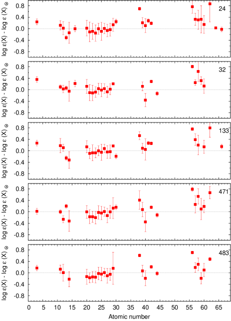
Figure 5: Differences between the chemical abundances of the G-type giants 24, 23, 133, 471, and 483, and the Sun.

Table 9: The changes of $\rm[Fe/H]$ resulting from the changes of $T_{\rm eff}$, $\log g$, and $v_{\rm t}$.

WEBDA (KIC)	$\Delta T_{\rm eff}$	$\Delta\log g$	$\Delta v_{\rm t}$
	$\pm 50$ K	$\pm 0.1$ dex	$\pm 0.5$ km s-1
24 (9655101)	$\pm 0.039$	$\pm 0.008$	$\mp 0.141$
32 (9655167)	$\pm 0.035$	$\pm 0.006$	$\mp 0.162$
133 (9716090)	$\pm 0.030$	$\pm 0.013$	$\mp 0.095$
471 (9776739)	$\pm 0.030$	$\pm 0.009$	$\mp 0.144$
483 (9532903)	$\pm 0.027$	$\pm 0.018$	$\mp 0.121$

The general pattern of abundances in our programme stars is consistent with solar values by Grevesse & Sauval (1998) as shown in Fig. 5. Slightly higher differences between abundances derived in this paper, and the solar values can be noticed for a few rare-earth elements for which only few lines were available for analysis, and for Ba which we find overabundant and which we discuss in a next paragraph.

In the last column of Table 8, we provide the weighted mean ratios of chemical elements to iron for the whole cluster calculated from the individual values measured for the five G-type stars. If all individual measurements of an element has an uncertainty given in Table 8, then the column ’cluster mean’ provides a weighted mean and uncertainty. If, for a given element, any star in Table 8 had a measurement without an uncertainty, we used a flat mean and the star-to-star RMS scatter as the uncertainty. In the case of Gd where there was only one measurement, we do not provide an uncertainty for the cluster mean.

Most of these values are very close to solar, however, there are few exceptions. We comment upon some of them in the following, cautioning the reader to keep in mind the difficulty of comparing results from different spectroscopic studies. One of those exceptions is a very high abundance of barium (the mean value for the cluster $\rm[Ba/Fe]=0.71\pm 0.03$) which may be expected in the youngest clusters but not in the oldest (see D’Orazi et al., 2009). Indeed, there is very few open clusters of an age similar to NGC 6811 and a comparably high abundance of barium: NGC 2324, $age=0.67$ Gyr (Salaris et al., 2004), $\rm[Ba/Fe]=0.66\pm 0.09$ (D’Orazi et al., 2009) and an even older cluster NGC 2141, $age=2.45$ Gyr (Salaris et al., 2004), $\rm[Ba/Fe]=0.91$ derived by Young et al. (2005) (but see Jacobson & Friel, 2013, who obtained a value lower by a half). Therefore, we conclude that even though the Ba abundance which we report is high, it is still consistent with other open clusters of an age near 1 Gyr.

In Fig. 6 we plot the synthetic and the observed spectra of stars 24, 32, 133, 471, and 483, centred at the lines of barium which have been analysed by us. For star 24, we show all the lines of Ba which were used in our analysis. All those lines yielded consistent abundance of barium. That concerns also the line of Ba II at 4934.077 Å  which shows slight asymmetry due to difficulties in the continuum placement. For the other stars, where fewer lines were measured, we show only the fit of a Ba II line at 5853.675Å. Like for the other elements, the abundance of Ba has been derived from all available spectral features. Our computations included the hyperfine splitting.

Another interesting element is zirconium. Our ratio of $\rm[Zr/Fe]=-0.22\pm 0.16$ is lower than expected for a 1 Gyr-old open cluster according to figure 9 of Maiorca et al. (2011) and as such is more consistent with the conclusion of Jacobson & Friel (2013) that [Zr/Fe] shows no trend with age. Finally, we report that the abundance of Li in all the five G-type stars has been found to be higher than expected for red clump stars (c.f., e.g., Villanova et al., 2010; Gonzalez et al., 2009). We note, however, that the respective spectral region at 6707.76 Å and 6707.91 Å where the spectral features of Li are located was found to be useless in the data acquired on 28 June 2007 for all stars but 24. Therefore, our determination of the abundance of lithium in red clump stars in NGC 6811 should be taken with caution.

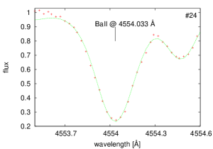
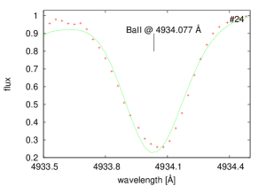
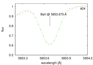
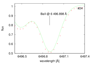
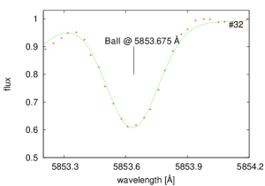
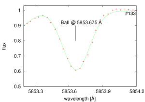
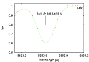
Figure 6: The synthetic and the observed spectra of stars 24, 32, 133, 471, and 483, centred at the lines of Ba analysed in this paper. For star 24, we show all the Ba lines used in the analysis. For the remaining stars, only the Ba II line at 5853.675 Å  is shown. The observed spectra are plotted with crosses while the synthetic ones are plotted with a solid line. The position of Ba lines are indicated. The star numbers are indicated in the right top corner of each panel.

Table 10: Properties of red clump stars in NGC 6811.

Property	WEBDA (KIC)					Average
	24 (9655101)	32 (9655167)	133 (9716090)	471 (9776739)	483 (9532903)
$\nu_{\rm{max}}$ [$\mu$Hz]	$98.2\pm 2.4$	$100.3\pm 8.7$	$101.4\pm 5.9$	$93.4\pm 9.0$	$96.3\pm 4.5$	–
$\Delta\nu$ [$\mu$Hz]	$7.86\pm 0.04$	$8.07\pm 0.04$	$8.56\pm 0.06$	$7.93\pm 0.16$	$7.69\pm 0.16$	–
$T_{\rm{eff}}$ [K]	$5005\pm 100$	$4924\pm 100$	$4980\pm 100$	$4952\pm 100$	$5008\pm 100$	–
$V$	11.236	11.318	11.372	11.159	11.172	–
From asteroseismic scaling relations:
$M/M_{\odot}$	$2.23\pm 0.18$	$2.09\pm 0.66$	$1.73\pm 0.33$	$1.82\pm 0.60$	$2.30\pm 0.39$	$2.12\pm 0.14$
$R/R_{\odot}$	$8.70\pm 0.25$	$8.36\pm 0.74$	$7.55\pm 0.46$	$8.08\pm 0.85$	$8.91\pm 0.58$	$8.47\pm 0.19$
$(m-M)_{\rm v}$	$10.32\pm 0.15$	$10.22\pm 0.24$	$10.12\pm 0.19$	$10.02\pm 0.27$	$10.32\pm 0.19$	$10.23\pm 0.08$
From alternative approach:
$\delta\nu_{\rm{max}}$ [$\mu$Hz]	1.00	3.30	10.05	7.52	0.03	–
$M/M_{\odot}$ (fixed)	2.30	2.30	2.30	2.30	2.30	2.30
$R/R_{\odot}$	8.79	8.63	8.30	8.74	8.92	8.68
$(m-M)_{\rm v}$	10.34	10.29	10.33	10.19	10.32	10.29

7 Cluster parameters

With our spectroscopic measurements of metallicity and effective temperatures, a detailed asteroseismic investigation of the cluster stars can now begin. Although this is beyond the scope of the present paper, we can already make some inferences on the cluster properties by utilising our spectroscopic measurements and the asteroseismic measurements of the helium burning red clump (RC) stars available at this point. We calculated the masses, radii and apparent distance moduli from the asteroseismic scaling relations in the form of eqns. (3) and (4) of Miglio et al. (2012). The input values for these calculations are given in the top part, and results in the middle part of Table 10. We adopted the $T_{\rm{eff}}$ values derived with the code SME with $\log g$ fixed at the asteroseismic value, and an uncertainty of $\pm$100 K consistent with the biases reported in Table 4. The choice of using results from SME was based mainly on the low star-to-star scatter in $\rm[Fe/H]$ values obtained from that code. We note however that the cluster parameters derived in this section would only be affected at a level below the $1\,\sigma$ uncertainties by adopting the FITSUN values instead. The abundances of other elements than Fe were only measured with FITSUN and we adopt the scaled solar result. Since these are measurements relative to Fe, this result will not be significantly affected by differences in the stellar parameters at the level we find between methods. The $V$-band magnitudes used in these computations were adopted from Glushkova, Batyrshinova & Ibragimov (1999).

Due to rather large uncertainties, on $\nu_{\rm max}$ in particular, the masses of the RC stars are not as precisely determined as we would like when calculated from the asteroseismic scaling relations. Therefore, we also adopted the alternative approach of estimating the asteroseismic RC masses from figure 4 of Stello et al. (2013). In that figure, valid for solar metallicity, it can be seen that the maximum value of $\Delta\nu$ for a helium core-burning star defines the mass of the star, regardless of the $\Delta P$ value. From the maximum value of $\Delta\nu$ for our stars in Table 2 (8.56 $\mu$Hz), we obtain a RC mass of 2.3 $M_{\odot}$.

When comparing this number to the individual mass measurements done using the scaling relations, we find that they are in agreement within the uncertainties. For the latter determinations, we find that the errors in mass and apparent distance modulus are correlated along a line defined by uncertainties in $\nu_{\rm max}$ which has also been found by Brogaard et al. (2014) for the open cluster NGC 6819. We only expect a very small systematic correction to $\Delta\nu$ in the case of the RC stars with mass and $T_{\rm{eff}}$ appropriate for NGC 6811 (see figure 2 in Miglio et al., 2013). Therefore, since the main source of the random uncertainty of mass comes from $\nu_{\rm max}$, we slightly adjusted the values of $\nu_{\rm max}$ for each star until the masses from the scaling relations resulted in 2.3 $M_{\odot}$, consistent with our alternative approach. These corrections ($\delta\nu_{\rm max}$) were always positive but much less than $1\sigma$ for three stars, $0.8\sigma$ for one star and $1.7\sigma$ for another star. We then calculated the radii and apparent distance moduli of the stars using the corrected values of $\nu_{\rm max}$. By doing that, the asteroseismic distance moduli from the individual stars reach a much better agreement, as they should, since all cluster stars are expected to be at the same distance. The numbers from this alternative approach are given in the bottom part of Table 10.

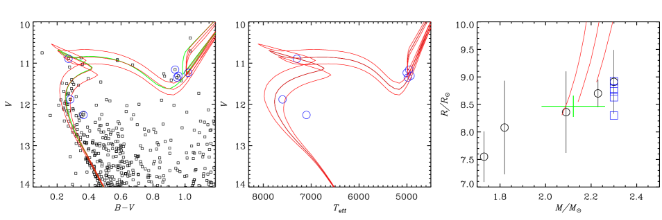
Figure 7: Left: the $(B-V)-V$ colour-magnitude diagram of NGC 6811 from Janes et al. (2013). Blue circles indicate cluster members identified in this paper. The isochrones of 0.9, 1.0, and 1.1 Gyr and $\rm[Fe/H]=+0.05$ from Bressan et al. (2013) are overplotted in red. The green line indicates the 1.0 Gyr isochrone transformed to the observational plane using MARCS atmosphere models instead of the colour-transformations adopted by Bressan et al. (2013). Middle: $T_{\rm eff}-V$ diagram of NGC 6811; blue circles indicate the same cluster members as on the left panel. Right: the masses and radii of the RC stars as determined from the scaling relations (black circles) and from our alternative approach (blue squares). The weighted mean value and its $1\sigma$ uncertainty is indicated by the green plus sign. The RC stage of isochrones of 0.9, 1.0, and 1.1 Gyr with ages increasing from right to left are overplotted.

On the left panel of Fig. 7, we show the $(B-V)-V$ colour-magnitude diagram (CMD) of NGC 6811 from the observations of Janes et al. (2013). Our RC stars and hot single cluster members with no spectroscopic evidence for binarity (stars 33, 54 and 528; Table 1) are indicated with blue circles, and PARSEC isochrones (Bressan et al., 2013) having $[Fe/H]=+0.05$ and ages of 0.9, 1.0, and 1.1 Gyr, respectively, are shown. To put the isochrones on the observational plane, we used an apparent distance modulus of 10.29 mag calculated from our spectroscopic $T_{\rm eff}$ measurements obtained with SME for the asteroseismic $\log g$ values (see the middle right-hand part of Table 3), the bolometric corrections from MARCS atmosphere models (Casagrande & VandenBerg, 2014) and the asteroseismic measurements from Table 2 with $\nu_{\rm max}$ slightly corrected as described above (see Table 10.) A reddening of $E(B-V)=0.05$ was applied to the isochrones in an attempt to match the observed main sequence. In order to get the best reddening estimate, we assumed that our three hot single member stars should have the same position relative to the isochrone on colour and $T_{\rm eff}$ planes by comparing the left and middle parts of Fig. 7. The faintest of the hot stars (star 54) appears to be an equal mass binary from its location in the left and middle panels, although we found no clear spectroscopic evidence for that. However, the star can still be used for our procedure, since we are only requiring the position of the star relative to the isochrone to be similar in the left and middle panels. As explained below, we could not use the RC stars for this even though they appear to match the isochrones better than the hot stars in the middle panel of Fig. 7.

To emphasise the effects of different colour-temperature calibrations, in the left panel of Fig. 7, we use a green line to plot the 1 Gyr isochrone translated to colours with the bolometric corrections from MARCS atmosphere models that were also used to calculate the apparent distance modulus, in addition to the colours that come with the PARSEC isochrones which are plotted in red. As seen, the predicted colour of the RC is significantly different in these two cases. The remaining parts of the two 1 Gyr isochrones show very little difference. This illustrates one of the problems of estimating cluster reddening and other parameters by comparing observed and synthetic colours. This issue of not knowing whether colour-$T_{\rm eff}$ transformations predict a correct colour-difference between the main sequence and the RC can significantly bias results from isochrone fitting in the absence of spectroscopic constraints. We suspect that this is the major reason why Janes et al. (2013) found a lower metallicity for NGC 6811 from photometry, as we have checked that a lower metallicity isochrone predicts a smaller separation between the unevolved main sequence and the RC.

One might be tempted to rely on the MARCS transformations, since they appear to show better consistency between colour and $T_{\rm eff}$ when comparing the left and middle panels, but that might just be a coincidence caused by inaccuracies in stellar models coupled to the uncertainty of our measurements and the photometry. In any case, if we were to make use of the RC stars to estimate the reddening, we would obtain a reddening which is lower than what the main sequence suggests, $E(B-V)\sim 0.03$ using the MARCS colour-transformations, or a reddening close to zero if we trust the colours that come with the PARSEC isochrones. Although the reddening seems to be rather uncertain, a much higher reddening of $E(B-V)=0.16$ suggested for the cluster by Schlegel et al. (1998) is clearly too high, since such a high value would make it impossible to match the CMD with an isochrone given our constraints on $T_{\rm eff}$, [Fe/H], and apparent distance modulus. This explains why Hekker et al. (2011), who based their analysis on photometric $T_{\rm eff}$ values obtained by assuming $E(B-V)=0.16$, obtained an $\rm[Fe/H]$ value for the cluster that is much too low.

The isochrones of age 0.9, 1.0, and 1.1 Gyr match the CMD about equally well, with a slight preference towards 1 Gyr, although that depends rather strongly on the interpretation of the brightest blue stars, which itself depends on the amount of convective core overshoot assumed in the stellar models. Ages older than 1.1 Gyr and younger than 0.9 Gyr seem to be disfavoured by the CMD, although a different amount of convective core overshoot would allow a slightly larger range of ages.

In the right panel of Fig. 7, we show the masses and radii of the RC stars as determined from the scaling relations in black with the weighted mean value and its $1\sigma$ uncertainty marked by the green plus, and measurements from our alternative approach in blue. We compare those to the RC phase of the same isochrones as in the other panels, with ages increasing from right to left. Uncertainties on mass measurements are not shown, but they are given in Table 10. As can be seen, the inferred age of the cluster depends on which of the asteroseismic mass measurements we rely on but it is consistent with the range of ages inferred from the CMD. Although it is difficult to estimate the uncertainty on the mass measurements from our alternative approach, it seems most likely that the true masses of the RC stars are somewhere between the two estimates. Possible causes for their difference include potential small systematic corrections to the scaling relations, an underestimate of the $T_{\rm eff}$ values, and potential changes to the isochrones in fig. 4 in Stello et al. (2013) when including convective core overshoot.

A more detailed asteroseismic analysis should allow a more detailed analysis of the cluster and its evolved stars. Not only by making use of the much longer Kepler time series data that are now available for these stars, but also by measuring the individual oscillation frequencies instead of only the basic asteroseismic measures. The additional information that comes from analysis of detached eclipsing binaries that have been identified in the cluster (Brogaard et al., 2014) will also provide useful constraints. When all such measurements are available, the cluster will be extremely well characterised and should be well suited to obtain new constraints on convective core overshoot (Montalbán et al., 2013).

We summarise our derived properties of NGC6811 in Table 11. The average $\rm[Fe/H]$ has been calculated from the mean values obtained for G-type stars with the codes FITSUN, SME, and ROTFIT and reported in Table 4.

Table 11: Properties of NGC6811.

Cluster property	value
$\rm[Fe/H]$	$+0.04\pm 0.01$ dex (internal error)
$\rm[M/Fe]$	scaled solar
age	$1.0\pm 0.1$ Gyr
$(m-M)_{\rm V}$	$10.29\pm 0.14$ mag
$E(B-V)$	$0.05\pm 0.02$ mag
$\langle M_{\rm RC}\rangle$	$2.12\pm 0.14\,M_{\odot}$

8 Summary

We presented results of spectroscopic observations of 15 stars in the open cluster NGC 6811. The analysis of radial-velocities allowed us to discover five spectroscopic systems. We classified stars 68 and 173 as SB2, stars 24 and 489, as SB1 candidates, and star 218, as SB1. The mean radial-velocity of the cluster derived in this paper is $+6.68\pm 0.08$ km s^-1.

Eight stars have been classified as confirmed or very probable cluster members and three, to be non-members. For stars 68, 113, 218, and 489 which are either spectroscopic binaries or $\delta$ Sct variables, or both, membership was not assessed. The atmospheric parameters and the projected rotational velocity have been derived for 13 stars.

The red clump of NGC 6811 consists of at least six stars; stars 471 and 483 were classified as RC in this paper while stars 24, 32, and 133 have been classified as RC by Mermilliod & Mayor (1990). The sixth star, KIC 9534041, was classified as RC by Stello et al. (2011). For the five RC stars in our sample, the abundances of 34 chemical elements have been computed. The mean mass of the red clump stars in the cluster has been found to be $2.12\ pm0.14M_{\odot}$

We showed that the mean metallicity of NGC 6811 is close to solar, and that the pattern of most elements in this cluster agrees with typical values observed for the Galactic open clusters of similar age and location. An exception is barium which we find to be overabundant.

The age of NGC 6811 has been found to be $1\pm 0.1$ Gyr.

References

- Becker (1947) Becker W., 1947, Astronomische Nachrichten, 275, 229
- Bergemann (2011) Bergemann M., 2011, MNRAS, 413, 2184
- Bergemann & Cescutti (2010) Bergemann M., Cescutti G., 2010, A&A, 522, A9
- Bergemann & Gehren (2008) Bergemann M., Gehren T., 2008, A&A, 492, 823
- Bergemann et al. (2012a) Bergemann M., Hansen C. J., Bautista M., Ruchti G., 2012, A&A, 546, A90
- Bergemann et al. (2012b) Bergemann M., Kudritzki R.-P., Plez B., Davies B., Lind K., Gazak Z., 2012, ApJ, 751, 156
- Bergemann et al. (2012c) Bergemann M., Lind K., Collet R., Magic Z., Asplund M., 2012, MNRAS, 427, 27
- Borucki et al. (2003) Borucki W. J. et al., 2003, in Society of Photo-Optical Instrumentation Engineers (SPIE) Conference Series, Vol. 4854, Society of Photo-Optical Instrumentation Engineers (SPIE) Conference Series, ed. J.C. Blades, O.H.W. Siegmund, 129-140
- Bressan et al. (2013) Bressan A., Marigo P., Girardi L., Nanni A., Rubele, S., 2013, 40th Liège International Astrophysical Colloquium ”Ageing Low Mass Stars: From Red Giants to White Dwarfs”, Liège, Belgium, Eds. J. Montalbán, A. Noels, V. Van Grootel, EPJ Web of Conferences, Volume 43, id.03001
- Brogaard et al. (2012) Brogaard K. et al., 2012, A&A, 543, A106
- Brogaard et al. (2014) Brogaard K. et al., 2014, ’Asteroseismology of Stellar Populations in the Milky Way’, Ap&SS Proc., Springer, Eds.: A. Miglio, P. Eggenberger, L. Girardi, J Montalban
- Brown et al. (2011) Brown T. M., Latham D. W., Everett M. E., Esquerdo G. A., 2011, AJ, 142, 112 (http://cdsarc.u-strasbg.fr/viz-bin/Cat?V/133)
- Bruntt et al. (2010) Bruntt H., et al., 2010, MNRAS, 405, 1907
- Bruntt et al. (2012) Bruntt H., et al., 2012, MNRAS, 423, 122
- Casagrande & VandenBerg (2014) Casagrande L., VandenBerg D. A., 2014, MNRAS 444, 392
- Cesetti et al. (2013) Cesetti M., Pizzella A., Ivanov V. D., Morelli L., Corsini E. M., Dalla Bontà E., 2013, A&A, 549, A129
- Corsaro et al. (2012) Corsaro E. et al., 2012, ApJ, 757, 190
- Cutri et al. (2003) Cutri R. M. et al., 2003, The 2MASS All-Sky Catalog of Point Sources, University of Massachusetts and Infrared Processing and Analysis Center, IPAC/California Institute of Technology
- Debosscher et al. (2011) Debosscher J., Blomme J., Aerts C., De Ridder J., 2011, A&A 529, A89
- Dias, Lepine & Alessi (2002) Dias W. S., Lepine J. R. D., Alessi B. S., 2002, A&A, 388, 168
- D’Orazi et al. (2009) D’Orazi V., Magrini L., Randich S., Galli D., Busso M., Sestito P., 2009, ApJ, 693, L31
- Frandsen et al. (2013) Frandsen S. et al., 2013, A&A, 556, A138
- Frasca et al. (2003) Frasca A., Alcalà J. M., Covino E., Catalano S., Marilli, E., Paladino R., 2003, A&A, 405, 149
- Frasca et al. (2006) Frasca A., Guillout P., Marilli E., Freire Ferrero R., Biazzo K., Klutsch A., 2006, A&A, 454, 301
- Frinchaboy & Majewski (2008) Frinchaboy P. M., Majewski S. R., 2008, AJ, 136, 118
- Glushkova, Batyrshinova & Ibragimov (1999) Glushkova E. V., Batyrshinova V. M., Ibragimov M. A., 1999, Astronomy Letters, 25, 86
- Gómez Maqueo Chew et al. (2013) Gómez Maqueo Chew Y. et al., 2013, ApJ, 768, 79
- Gonzalez et al. (2009) Gonzalez O. A. et al., 2009, A&A, 508, 289
- Grevesse & Sauval (1998) Grevesse N., Sauval A. J., 1998, Sp. Sci. Rev., 85, 161
- Grevesse, Asplund & Sauval (2007) Grevesse N., Asplund M., Sauval A. J., 2007, Sp. Sci. Rev., 130, 105
- Grupp (2004a) Grupp F., 2004, A&A, 420, 289
- Grupp (2004b) Grupp F., 2004, A&A, 426, 309
- Gustafsson et al. (2008) Gustafsson B., Edvardsson B., Eriksson K., Jørgensen U. G., Nordlund Å, Plez B., 2008, A&A, 486, 951
- Hekker et al. (2011) Hekker S. et al., 2011, A&A, 530, A100
- Jacobson & Friel (2013) Jacobson H. R., Friel E. D., 2013, AJ, 145, 107
- Janes et al. (2013) Janes K., Barnes S. A., Meibom S., Hoq S., 2013, AJ, 145, 7
- Kharchenko et al. (2004) Kharchenko N. V., Piskunov A. E., Röser S., Schilbach E., Scholz R.-D., 2004, Astron. Nach., 325, 740
- Kharchenko et al. (2005) Kharchenko N. V., Piskunov A. E., Röser S., Schilbach E., Scholz R.-D., 2005, A&A, 438, 1163
- Koch et al. (2010) Koch D. G. et al.,, 2010, ApJ, 713, L79
- Korn et al. (2003) Korn A. J., Shi J., Gehren T., 2003, A&A, 407, 691
- Kurucz (1993) Kurucz R., 1993, CD-ROM 18
- Lind et al. (2012) Lind K., Bergemann M., Asplund M., 2012, MNRAS, 427, 50
- Lindoff (1972) Lindoff U., 1972, å, 16, 315
- Luo et al. (2009) Luo Y. P., Zhang X. B., Luo C. Q., Deng L. C., Luo Z. Q., 2009, New Astronomy 14, 584
- Maiorca et al. (2011) Maiorca E., Randich S., Busso M., Magrini L., Palmerini S., 2011, ApJ, 736, 120
- Mermilliod & Mayor (1990) Mermilliod J. C., Mayor M., 1990, A&A, 237, 61
- Mermilliod, Mayor & Udry (2008) Mermilliod J. C., Mayor M., Udry S., 2008, A&A, 485, 303
- Metcalfe et al. (2010) Metcalfe T. S. et al., 2010, ApJ, 723, 1583
- Miglio et al. (2012) Miglio A. et al., 2012, MNRAS, 419, 2077
- Miglio et al. (2013) Miglio A. et al., 2013, 40th Liège International Astrophysical Colloquium ”Ageing Low Mass Stars: From Red Giants to White Dwarfs”, Liège, Belgium, Eds. J. Montalbán, A. Noels, V. Van Grootel, EPJ Web of Conferences, Volume 43, id.03004
- Molenda-Żakowicz et al. (2010) Molenda-Żakowicz J., Jerzykiewicz M., Frasca A., Catanzaro G., Kopacki G., Latham D. W., 2010, arXiv 1005.0985
- Molenda-Żakowicz et al. (2013) Molenda-Żakowicz J. et al., 2013, MNRAS, 434, 1422
- Montalbán et al. (2013) Montalbán J., Miglio A., Noels A., Dupret M.-A., Scuflaire R., Ventura P., 2013, ApJ, 766, 118
- Niemczura, Morel & Aerts (2009) Niemczura E., Morel T., Aerts C., 2009, A&A, 506, 213
- Önehag et al. (2011) Önehag A., Korn A., Gustafsson B., Stempels E., Vandenberg D. A., 2011, A&A, 528, A85
- Pancino et al. (2010) Pancino E., Carrera R., Rossetti E., Gallart C., 2010, A&A, 511, A56
- Prugniel & Soubiran (2001) Prugniel Ph., Soubiran C., 2001, A&A, 369, 1048
- Prs̆a et al. (2011) Prs̆a A. et al., 2011, AJ, 141, 83
- Salaris et al. (2004) Salaris M., Weiss A., Percival S. M., 2004, A&A, 414, 163
- Sanders (1971) Sanders W. L., 1971, A&A, 15, 368
- Sandquist et al. (2013) Sandquist E. L. et al., 2013, AJ, 146, 40
- Santos, Israelian & Mayor (2004) Santos N. C., Israelian G., Mayor M., 2004, A&A, 415, 1153
- Sbordone (2005) Sbordone L., 2005, MSAIS, 8, 61
- Schlegel et al. (1998) Schlegel D. J., Finkbeiner D. P., Davis M., 1998, ApJ, 500, 525
- Shi et al. (2014) Shi J. R., Gehren T., Zeng J. L., Mashonkina L., Zhao G., 2014, ApJ, 782, 80
- Sousa et al. (2006) Sousa S. G., Santos N. C., Israelian G., Mayor M., Monteiro M. J. P. F. G., 2006, A&A, 458, 873
- Sousa et al. (2008) Sousa S. G., et al., 2008, A&A, 487, 373
- Sousa et al. (2011a) Sousa S. G., et al., 2011a, A&A, 526, A99
- Sousa et al. (2011b) Sousa S. G., et al., 2011b, A&A, 533, A141
- Stello et al. (2009) Stello D., Chaplin W. J., Basu S., Elsworth Y., Bedding T. R., 2009, MNRAS, 400, L80
- Stello et al. (2011) Stello D. et al., 2011, ApJ, 739, 13
- Stello et al. (2013) Stello D. et al., 2013, ApJ Letters, 765, L41
- Thygesen et al. (2012) Thygesen A. O., et al., 2012, å, 543, 160
- Tonry & Davis (1979) Tonry J., Davis M., 1979, AJ, 84, 1511
- Topping (1972) Topping J., 1972, Errors of Observation and Their Treatment, Chapman Hall Ltd., 92
- Udry et al. (1999) Udry S. et al., 1999, in Precise Stellar Radial Velocities ASP Conf. Ser., 185, 383
- Uytterhoeven et al. (2010b) Uytterhoeven K. et al., 2010a, AN, 331, poster P30 (arXiv:1003.6089)
- Uytterhoeven et al. (2010a) Uytterhoeven K. et al., 2010b, AN, 331, 993
- Uytterhoeven et al. (2011) Uytterhoeven K. et al., 2011, A&A, 534, 125
- Valdes et al. (2004) Valdes F., Gupta R., Rose J. A., Singh H. P., Bell D. J., 2004, ApJS, 152, 251
- Valenti & Piskunov (1996) Valenti J. A., Piskunov N., 1996, A&AS, 118, 595
- Van Cauteren et al. (2005) Van Cauteren P., Lampens P., Robertson C. W., Strigachev A., 2005. CoAst, 146, 21
- Villanova et al. (2010) Villanova S., Randich S., Geisler D., Carraro G., Costa E., 2010, A&A, 509, A 102
- Watson, Henden & Price (2006) Watson C., Henden A. A., Price A., 2006, The AAVSO International Variable Star Index (Version 2011-04-17), Soc. for Astron. Sci. Ann. Symp. 25, 47
- Wong & Meibom (2009) Wong A., Meibom S., 2009, American Physical Society, Joint Fall 2009 Meeting of the Ohio Sections of the APS and AAPT, October 9-10, 2009, poster P1.006
- Young et al. (2005) Yong D., Carney B. W., Teixera de Almeida M. L., 2005, AJ, 130, 597